the Creative Commons Attribution 4.0 License.
the Creative Commons Attribution 4.0 License.
 | 19 Nov 2019
Hyper-resolution ensemble-based snow reanalysis in mountain regions using clustering
Joel Fiddes
Kristoffer Aalstad
Sebastian Westermann
Spatial variability in high-relief landscapes is immense, and grid-based models cannot be run at spatial resolutions to explicitly represent important physical processes. This hampers the assessment of the current and future evolution of important issues such as water availability or mass movement hazards. Here, we present a new processing chain that couples an efficient sub-grid method with a downscaling tool and a data assimilation method with the purpose of improving numerical simulation of surface processes at multiple spatial and temporal scales in ungauged basins. The novelty of the approach is that while we add 1–2 orders of magnitude of computational cost due to ensemble simulations, we save 4–5 orders of magnitude over explicitly simulating a high-resolution grid. This approach makes data assimilation at large spatio-temporal scales feasible. In addition, this approach utilizes only freely available global datasets and is therefore able to run globally. We demonstrate marked improvements in estimating snow height and snow water equivalent at various scales using this approach that assimilates retrievals from a MODIS snow cover product. We propose that this as a suitable method for a wide variety of operational and research applications where surface models need to be run at large scales with sparse to non-existent ground observations and with the flexibility to assimilate diverse variables retrieved by Earth observation missions.
- Article
(4062 KB) - Full-text XML
- BibTeX
- EndNote


Accurate simulation of energy and water cycles in high mountain environments is critical for a wide range of operational and research applications related to water resources and natural hazards, particularly in the current era of dramatic changes in mountain regions worldwide (Mankin et al., 2015). However, basic surface variables in many remote mountain areas remain poorly quantified despite large increases in the capacity of in situ observations, remote sensing platforms and atmospheric model products. Spatial resolutions of 100 m are commonly recommended for modelling of land surface variables such as snow cover or surface temperature in complex terrain (Bierkens et al., 2015; Wood et al., 2011; Baldo and Margulis, 2018) and has come to be known as hyper-resolution (Wood et al., 2011). This is due to the fact that energy and mass fluxes exhibit strong lateral variation due to the effects of topography (Gruber and Haeberli, 2007), and surface/subsurface properties such as vegetation cover (Shur and Jorgenson, 2007), ground material (Gubler et al., 2012) or snow distribution (Zhang, 2005; Liston, 2004) further compound these effects.
Most continental to global modelling studies operate on regular grids which has placed limitations on model resolutions despite advances in computing power. However, previous efforts using hydrological response units, HRUs (Beven and Kirkby, 1979; Durand et al., 1993; Fiddes and Gruber, 2012), triangular irregular networks (Mascaro et al., 2015; Tucker et al., 2001), or multi-resolution approaches (Baldo and Margulis, 2018) suggest that regular grids are not only expensive but suboptimal as often only subsets of watersheds require detailed model descriptions in order to characterize the system adequately. In addition, deterministic modelling schemes have limitations even at hyper-resolution due to errors in forcing data, particularly regarding fields such as precipitation which suffer from both measurement and modelling biases.
The numerical weather prediction (NWP) community has been addressing this problem for several decades using various data assimilation (DA) approaches. DA methods, often with Bayes' rule as a starting point, attempt to ingest uncertain observations into uncertain model simulations (Lahoz and Schneider, 2014; Carrassi et al., 2018). It is a class of methods that are implicitly Bayesian in that uncertainty in both the simulation and observation are accounted for. These methods are diverse in design and application and the reader is directed to Liu et al. (2012) for a review relevant to the land surface community or Carrassi et al. (2018) for a timely overview. While DA has a long history as a tool employed in NWP (cf. the European Centre for Medium-Range Weather Forecast, ECMWF, and the North American Land Data Assimilation System, NLDAS), only relatively recently has data assimilation started to be utilized in land surface modelling schemes (Liu et al., 2012); however, it has already shown much promise in the current era of plentiful remote sensing data. In recent years, ensemble-based DA has been successfully applied to the problem of improving snowpack estimates at various spatial scales (Margulis et al., 2015; Aalstad et al., 2018; Magnusson et al., 2017; Griessinger et al., 2016); this is particularly pertinent as it is widely recognized that estimating the spatial distribution of the snow water equivalent (SWE) in mountain regions is currently one of the most important unsolved problems in snow hydrology (Dozier et al., 2016) and in understanding the spatial distribution of other processes dependent on the snowpack mass balance, such as the surface energy balance.
Ensemble-based data assimilation revolves around the use of an ensemble (i.e. a collection) of model trajectories. Each trajectory is referred to as an ensemble-member or particle, for economy we will use the latter. An ensemble allows for the quantification of uncertainty through the prior (before assimilation) and posterior (after assimilation) distribution of particles. The use of an ensemble increases the computational burden, often adding orders of magnitude to computation times. Given that computation time is practically limited, in ensemble simulation there is always a trade-off between a model's spatio-temporal resolution and the number of particles. Both are desirable, given that higher spatio-temporal resolution (presumably) increases model realism whereas a higher number of particles allows for improved uncertainty estimation. This is why the dual quest for efficiency in models and DA is important. We argue that some of the resources that are spent on explicit high-resolution spatial modelling could sometimes be better spent on the ensemble. When discussing computational expense, it is worth noting that the intended application is important to consider. Given a large high performance computing infrastructure and enough time, we currently have the ability to use brute force deterministic numerical simulations to solve many resource-intensive problems. However, the question is (a) what better purposes could that computation time be used for (e.g. uncertainty quantification) and (b) are we producing a final product (where one-off large simulations are tolerable) or as is more commonly the case, at least in research (but also operational centres), are we part way through a development cycle where we expect to make many iterations in order to gain knowledge of the system. In this second case there is a strong motivation for methods that allow quick development cycles and knowledge gain. The previously published TopoSUB and TopoSCALE models (Fiddes and Gruber, 2012, 2014) are highly efficient approaches that may provide a solution for this problem, particularly in data-sparse regions. TopoSUB is a sub-grid method that permits order of magnitude efficiency gains in applying numerical models over large areas. It achieves this by using a multivariate clustering of input predictors (normally topographical parameters) to reduce the number of simulations required to accurately represent surface heterogeneity by orders of magnitude. TopoSCALE provides point-scale meteorological forcing at any given point on the Earth's surface by downscaling gridded reanalysis (or other atmospheric model data) using pressure levels to account for gradients with elevation and topographic correction for surface energy balance terms. The computational resources saved by not simulating domains explicitly in 2-D can then be redirected to ensemble simulation for the purpose of data assimilation or uncertainty analysis in general. This approach has been successfully used to generate a regional-scale permafrost map at a 30 m resolution (Fiddes et al., 2015).
In this paper we present a new processing chain that couples an efficient sub-grid method (TopoSUB), a downscaling tool (TopoSCALE) and a data assimilation method with the purpose of improving numerical simulation of ground surface processes at multiple spatial and temporal scales in ungauged basins. The novelty of the approach is that while we add 2 orders of magnitude of computational cost by using ensemble simulations, we save 4–5 orders of magnitude over explicitly simulating a high-resolution grid. This approach makes data assimilation at large spatio-temporal scales feasible. In addition, this approach utilizes only freely available global datasets and is therefore able to run globally.
Applications of this approach are numerous and diverse as it addresses three common bottlenecks: (a) availability of an appropriately downscaled forcing, (b) ability to apply complex models at high resolution over large areas and (c) addressing uncertainty in the model chain. Applications could, for example, include large-scale assessments of mass movements, glacier mass balance or snowpack water availability. By translating global climate model/regional climate model (GCM/RCM) results to the local slope-scale impacts with appropriate surface models, climate change impacts can be estimated at appropriate scales.
The modelling pipeline used in this study employs two previously described methods (1) TopoSUB (Fiddes and Gruber, 2012) and (2) TopoSCALE (Fiddes and Gruber, 2014). These tools are briefly described here for clarity; however, the reader is directed to the original publications for full details. An overview of the full tool chain is given in Fig. 1.
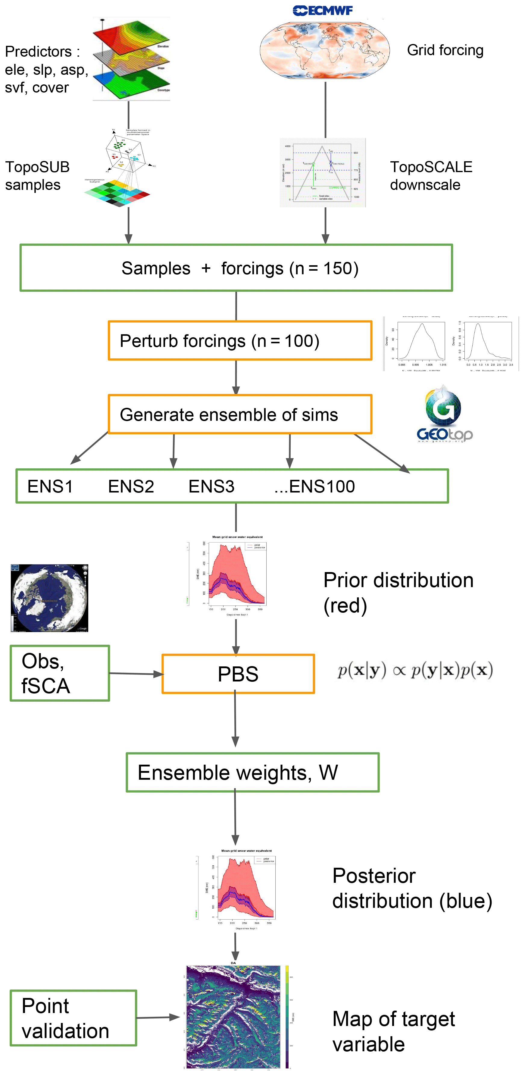
Figure 1Schematic of the modelling set-up. Input predictors are usually elevation (ele), slope (slp), aspect (asp), sky view factor (svf) and land cover (cover).
2.1 Surface model
The surface model used in this study, GEOtop, is a physically based model originally developed for hydrological research (Endrizzi et al., 2014). It couples energy and water budgets, represents the energy exchange with the atmosphere and has a multilayer snowpack. Further information is given by Bertoldi et al. (2006), Rigon et al. (2006), Endrizzi (2007) and Dall'Amico et al. (2011). A description of model uncertainty and sensitivity is given by Gubler et al. (2012). Model parameters and soil stratigraphy are set up as defined in Fiddes et al. (2015).
2.2 Downscaling forcing
TopoSCALE is a scheme that generates point-scale model forcing using gridded atmospheric model datasets. It achieves this as follows: (1) data available on pressure levels, including air temperature (Ta), relative humidity (RH), wind speed (U) and wind direction (φU) are interpolated to a point of interest in order to provide a dynamic scaling at each time step; (2) incoming longwave radiation (L↓) is scaled by accounting for downscaled Ta, RH and sky emissivity; (3) we apply a topographic correction to both radiation fields (); and (4) an elevation based lapse rate is applied to precipitation (P). The output is a full set of scaled meteorological fields required to drive a numerical model at hourly time steps.
2.3 Sub-grid scheme
TopoSUB is a scheme that samples land surface heterogeneity at high resolution based on a digital elevation model (DEM) and other surface data (here SRTM 3, 30 m). Input predictors describing dimensions of variability are clustered with a k-means algorithm to reduce computational units in a given simulation domain to a set of clusters. A 1-D surface model is then applied to each cluster using its mean physiographic properties. This approach allows savings in computational effort of multiple orders of magnitude over distributed approaches. For example, a simulation domain represented by an ERA5 grid cell (31 km × 31 km) contains approximately 106 SRTM 3 pixels. This domain can be simulated using 100 TopoSUB clusters, which represents a 104 reduction in the computational load during simulation.
2.4 Data assimilation
We build on previous efforts (e.g. Girotto et al., 2014; Margulis et al., 2015; Aalstad et al., 2018) that focus on the reanalysis of snowpack characteristics (particularly SWE and height of snow, HS) through ensemble-based assimilation of fractional snow covered area (fSCA) retrievals from optical satellite sensors. We choose to use fSCA retrievals because currently only optical satellite sensors can offer the resolution, coverage, accuracy and breadth of information needed to constrain snowpack simulations in complex terrain (see Dozier et al., 2016). We use fSCA retrieved from the MODIS sensors onboard the Aqua and Terra satellites. These retrievals have a sub-kilometric spatial resolution and a near-daily equatorial revisit frequency (in the absence of clouds); thus, the reanalysis we perform could be applied to any mountain range on Earth. By assimilating fSCA observations we exploit the dynamic information content contained in the depletion of the fractional snow cover. The idea is that if one grid cell melts out later than another, there must either have been more snow there to begin with, a slower ablation, or a combination of the two – and vice-versa for an earlier melt out (Martinec and Rango, 1981; Aalstad et al., 2018). This is the essence of traditional snow reconstruction where the snowpack is contrived in reverse from the observed date of disappearance of the snow cover to the day of peak SWE using modelled snowmelt rates (Martinec and Rango, 1981; Dozier et al., 2016). By using ensemble-based DA we can account for uncertainties in the remotely sensed fSCA depletion, the meteorological forcing and the snow model that are ignored in traditional reconstruction (Slater et al., 2013) and arrive at an improved reanalysis (Girotto et al., 2014). Snow reanalysis problems are best approached using batch smoother DA algorithms rather than the more commonly used filters as the snowpack has a long memory (i.e. high temporal autocorrelation) relative to (e.g.) synoptic-scale weather (Margulis et al., 2015; Aalstad et al., 2018). By using a smoother that assimilates all of the fSCA retrievals during the ablation season at once to constrain the ensemble of annual snowpack trajectories, we are able to use the observed ablation to inform the accumulation season which would not be possible with a particle filter.
2.4.1 Generating the prior ensemble
In line with previous studies (e.g. Raleigh et al., 2015), we assume that the main source of uncertainty in modelling the snowpack is in the meteorological forcing and specifically the main variables that control the mass and energy balance, namely air temperature (Ta), precipitation (P), and incoming shortwave (S↓) and longwave (L↓) radiation. To generate the prior ensemble we perturb the forcing time series using normally (Ta, S↓ and L↓) and lognormally (P) distributed multiplicative perturbation parameters that are fixed throughout the annual integration. Following Navari et al. (2016) we generate a correlated ensemble of perturbation parameters for the different forcing variables. This is to avoid unrealistic perturbations such as a large increase in both precipitation and shortwave radiation. We do this in two steps. First, we generate independent perturbation parameters for each of the forcing variables using normal and lognormal random draws. Secondly, we account for the correlation between the different perturbation parameters by performing a Cholesky decomposition of the covariance matrix. All hyper-parameters used in generating the prior ensemble are given in Table 1 and are based on values from a study in Colorado by De Lannoy et al. (2012) which, in turn, are based on the approach of Reichle et al. (2007), which is a global study.
Table 1Hyper-parameters (means, variances and correlations) defining the joint probability distribution from which the ensemble of multiplicative perturbation parameters are drawn (unitless). These parameters were obtained from De Lannoy et al. (2012) which, in turn, were based on the approach of Reichle et al. (2007).

2.4.2 Particle batch smoother
When performing DA we are usually interested in approximating the Bayesian posterior: the probability of model trajectories given the observations. The DA method employed in this study is the particle batch smoother (PBS) presented in the context of snow reanalysis in Margulis et al. (2015). The PBS is a basic importance sampling particle filter where no resampling takes place (see Van Leeuwen, 2009). This means that it is equivalent to the generalized likelihood uncertainty estimation (GLUE) with a formal likelihood function (Beven and Binley, 1992). The apparent advantage of this smoother is that, unlike the ensemble smoother (ES), it makes no assumptions about the linearity of the model or the Gaussianity of the error statistics (Van Leeuwen and Evensen, 1996). This can also be a disadvantage in higher-dimensional problems where the method is prone to degeneracy and large sampling error unless a very large number of particles is used (Van Leeuwen and Evensen, 1996; Van Leeuwen, 2009). Nonetheless, for snow reconstruction problems where the dimensionality of the parameter space is relatively low, the PBS has been shown to outperform the ES even with a moderate number of particles (Margulis et al., 2015; Aalstad et al., 2018). Crucially, using the PBS instead of the ES (or its iterative variants) avoids the need for running more than one ensemble model integration, which would be more costly and less aligned with the efficiency objectives of the clustering (TopoSUB) framework. As the PBS is derived elsewhere (Van Leeuwen and Evensen, 1996; Van Leeuwen, 2009; Margulis et al., 2015), here we are content with presenting the analysis equation for the posterior and how to implement it for the snow reconstruction problem. Each particle represents a different annual integration of the snow model and will have a unique forcing history associated with it as dictated by the perturbation parameters described in Sect. 2. An overview of the tool chain is given in Fig. 1. A priori, each of these histories is assumed to be equally likely. The observed fSCA depletion for the given water year and its assumed error structure is then used to constrain the ensemble of particles through the PBS analysis. In the PBS, the Bayesian posterior is approximated by a discrete probability mass function consisting of the posterior weights of each of the particles (model trajectories). As shown in Aalstad et al. (2018), when each particle is given an equal prior weight (1∕Ne) and a Gaussian likelihood is used, the posterior weight for the jth particle is given by
where Ne is the number of particles; the square norm of the innovations (residuals) for an arbitrary particle k is then given by
in which T denotes the matrix transpose, R is the observation error covariance matrix, y is the observation vector containing the remotely sensed fSCA depletion for a given snow season and is the predicted observation vector containing the corresponding modelled fSCA for particle k. The particle approximation of the Bayesian posterior represented by Eq. (1) improves as the number of particles increases. It should be clear from the analysis step in Eq. (1) that the posterior weights sum to one by definition. Furthermore, unlike the ES, the PBS only changes the relative weights of the particles and not their position within the model space. This makes the PBS particularly attractive in a clustering framework, as we do not need to rerun the ensemble after the analysis.
An important component of DA is the prescribed error covariance structure of the observations. As the MODIS fSCA retrievals that we are assimilating are affected by various error sources that vary from day to day, such as atmospheric conditions and viewing angle, we assume that the observation errors are uncorrelated in time. Moreover, we assume a fixed observation error variance . Thus, we use a simple scalar diagonal observation error covariance matrix , where I is the identity matrix in line with similar studies (e.g. Margulis et al., 2015; Aalstad et al., 2018). This simplifies Eq. (2) which reduces to a simple square sum of innovations normalized by a constant (). We prescribe an observation error standard deviation of σy=0.13 based on the estimate in Aalstad et al. (2018) (see Sect. 3.3). In order to make the model trajectories comparable to the fSCA retrievals during the analysis step, i.e. to generate the predicted observations , an observation operator is required. We use a simple threshold on SWE to determine the binary (snow/no-snow) snow cover of each modelled grid cell based on SWE values that correspond to full pixel coverage (fSCA = 1) given in Thirel et al. (2013); this allows us to consider surface roughness. Due to the scale difference between the MODIS pixels (500 m) and the model grid cells (3 m), the modelled fSCA within a MODIS pixel is then simply the average of the binary snow cover in all model grid cells that fall within that pixel.
3.1 Meteorological forcing
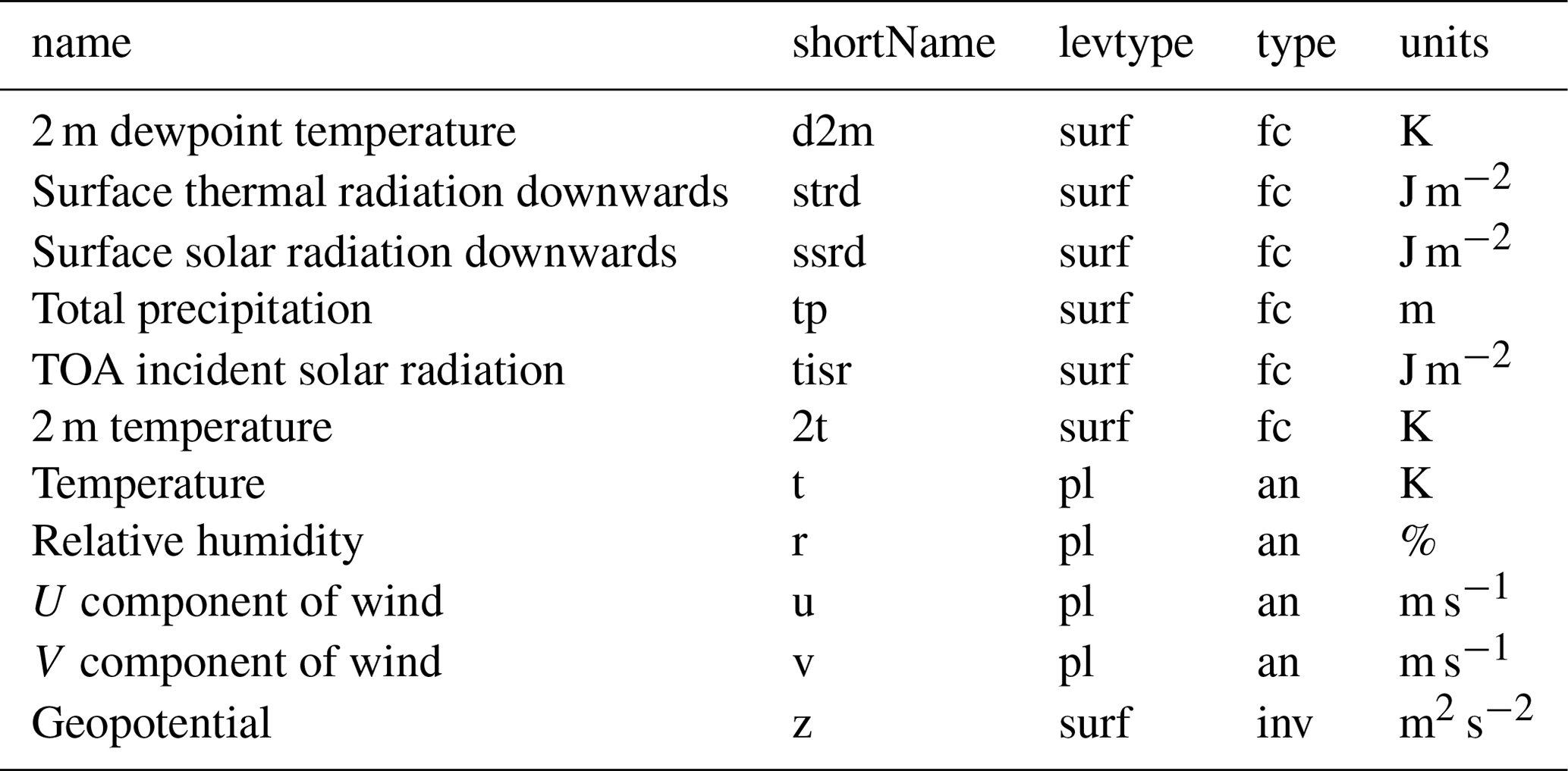
Driving climate data are obtained from the ERA5 reanalysis from ECMWF. This is the latest reanalysis from ECMWF that updates the ERA-Interim reanalysis. The main improvements are an increase in the spatial resolution to 31 km, hourly temporal resolution and an increase in the vertical model levels to 137. Accumulated values are now from the last time step and not from the last forecast as in ERA-Interim. This means that we can easily obtain the mean rates required to drive our numerical model by simply dividing these accumulations by the hourly time step (Fiddes and Gruber, 2014). Forcing data are detailed in Table 2. For each TopoSUB cluster, defined by the mean physiographic characteristics of a cluster, (Fiddes and Gruber, 2012) the ERA5 meteorological fields are downscaled using TopoSCALE (Fiddes and Gruber, 2014).
Table 2Description of the hourly fields obtained from the ERA5 reanalysis. All of the columns headers are terms defined by ECMWF. “levtype” refers to the level type, “surf” refers to the surface and “pl” denotes the pressure level. The “type” is either “fc”, which refers to forecast, “an”, which refers to analysis, or “inv”, which refers to invariant.
3.2 Surface properties
TopoSUB requires topographical parameters as input predictors to the clustering algorithm. We derive the following topographic parameters from the SRTM 3 digital elevation model: elevation, slope, aspect and sky view factor (proportion of visible sky). Surface cover is characterized in a simple three-mode classification in order to approximate subsurface stratigraphies: first a threshold on MODIS normalized difference snow index (NDSI) is used to classify vegetated surfaces, then a simple model further differentiates between steep bedrock and debris slopes. Further details are available in Fiddes et al. (2015).
3.3 Assimilated fSCA observations
We assimilate fSCA retrievals obtained from version 6 of the level 3 daily MODIS snow cover product from the Terra (MOD10A1 product; Hall and Riggs, 2016a) and Aqua (MYD10A1 product; Hall and Riggs, 2016b) satellites. The retrieval algorithm is based on the inversion of a linear regression of the MODIS NDSI on reference fSCA estimated from coincident Landsat imagery and it is given by the “FRA6T” relationship in Salomonson and Appel (2006). The normalized difference snow index exploits the fact that snow is highly reflective in the visible but a good absorber in the shortwave infrared which differentiates it from most other natural surfaces (Painter et al., 2009). If cloud-free retrievals are available from both Terra and Aqua retrievals for a given day then the Terra retrievals are used. Aalstad et al. (2018) compared MODIS fSCA retrievals to reference fSCA estimates obtained from time-lapse photography, imagery from an unmanned aerial vehicle and snow surveys at a site on Svalbard and obtained an RMSE of σy=0.13 for the MODIS retrievals. This estimate is in good agreement with those found in the Alps by other studies (e.g. Masson et al., 2018); thus, we use this as the observation error variance () in the assimilation (Sect. 2.3.2).
3.4 Evaluation
3.4.1 Station data
SWE (mm) measurements obtained manually by observers are available at approximate biweekly intervals from snow profiles across Switzerland. Here we use the GCOS dataset which consists of 11 sites (Fig. 2). We call these sites “stations” throughout the paper. The dataset is openly available (Marty, 2017). Automatic HS (cm) measurements performed by sonic ranger (Campbell Scientific SR50) are available from the Intercantonal Measurement and Information System (IMIS) station network at 30 min intervals. This is a high-elevation station network that forms the backbone of the national avalanche service in Switzerland.
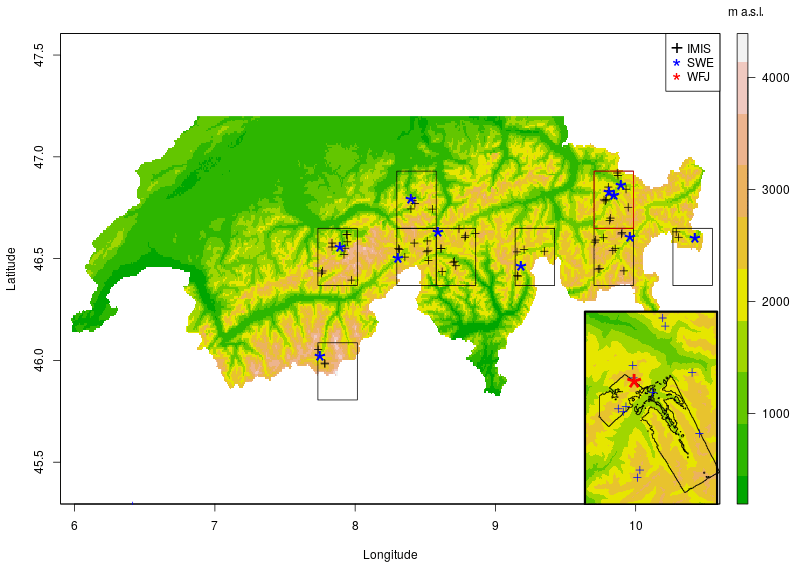
Figure 2Experimental set-up: the nine ERA5 grid boxes were selected based on the fact that they contained GCOS SWE monitoring sites (11 stations). All of the IMIS stations in each box are used for evaluation (39 stations). The Weissfluhjoch research station and the flight path of the ADS data are located in the red box, which is also shown at a larger scale in the inset.
3.4.2 Airborne snow height retrievals
The airborne digital sensor (ADS) optoelectronic line scanners ADS80 and ADS100 from Leica Geosystems were used to acquire summer and winter stereo images that were processed into high-resolution digital terrain models (DTMs) using photogrammetry (Bühler et al., 2015). HS is then retrieved by subtracting the summer DTM from the winter DTM and is available for two footprints in the Davos region covering the Wannengrat area (3.5 km ×7.5 km) and the Dischma area (7 km × 17 km) which comprise high Alpine terrain. The footprint of this survey is shown in Fig. 2. These data are used for the spatial evaluation of the scheme. Acquisition dates are 20 March 2012, 15 April 2013 and 17 April 2014. All snow depth maps were calculated using a summer DTM from 3 September 2013. The resolution of this dataset is 2 m with a vertical RMSE of around ±30 cm (Vögeli et al., 2016a; Bühler et al., 2015). The datasets are resampled to 100 m (Vögeli et al., 2016a) and are used here to evaluate the methods. Snow depth in areas covered with forest, scrub, buildings and water bodies can not be determined using the ADS (Bühler et al., 2015) and are therefore masked out from the datasets. This dataset is openly available (https://doi.org/10.16904/23; Vögeli et al., 2016b). Additionally, as only a single summer (2013) DTM was used, all glacier areas were masked out to avoid errors associated with changing glacier surfaces. Glacier outlines were obtained from the Global Land Ice Measurements from Space (GLIMS) repository (Raup et al., 2007).
In this study we conduct experiments at various spatio-temporal scales in order to comprehensively test the framework and assess its suitability for various applications. The experimental set-up is shown in Fig. 2. Simulations are run in nine ERA5 grid boxes spanning the Swiss Alps. Each grid box contains at least one SWE measurement location as well as several IMIS stations that are used to evaluate HS results. In addition we perform large area simulations on the entire Swiss Alps domain to explore how seasonal extremes are represented at the large scale.
A prerequisite for the first two experiments (Sect. 4.1–4.2) is the PBS analysis step, as described in Sect. 2, which generates the posterior weights matrix Wp based on PBS analysis units of MODIS cells. This then has the dimensions Ne×Np, where Ne is the number of particles (ensemble members) and Np is the number of MODIS pixels. The following describes how Wp is used to generate posterior estimates of a given state variable (SWE or HS). The third experiment (Sect. 4.3) differs in that the analysis unit is the ERA5 grid cell itself and aims to correct aggregated grid-level bias in forcing.
4.1 Point DA
Point-scale DA is accomplished by simply mapping the DEM cell corresponding to point of interest (e.g. a validation station) to the corresponding MODIS pixel for that location. The Wp derived from the PBS analysis for that MODIS pixel is then used directly to generate the posterior estimate for that point. Model state results are obtained from the TopoSUB cluster that the DEM cell is a member of. Cumulative distributions of state variables are computed through the ranking of the ensemble of state variables followed by a cumulative summation of the correspondingly sorted weights. These distributions allow for the estimation of quantile values of the posterior model state.
4.2 Spatially distributed DA
The particle batch smoother has typically been applied at the point scale or on regular grids. Here we generalize the method so as to fit the TopoSUB approach. The basic aim is to generate posterior weights for each TopoSUB cluster (which has no location, only physiographic attributes) so that the weights can be used in a highly scalable and powerful manner to generate different products such as a time series of the posterior median aggregated to give basin-level statistics. The key challenge in this aim is how to map the spatial unit of the PBS algorithm, the MODIS pixel, which has a location in space, to a TopoSUB cluster which does not. We achieve this via the following:
where Wp is the Ne×Np weights matrix and a is a Np×1 vector containing the fractional abundance (cover) of cluster c represented in each of the MODIS pixels. Here wc contains the weight of each forcing history for cluster c and is computed for each of the clusters. This yields the weights matrix wc that contains the weights of the forcing histories for each cluster. As a second step the weights wc are renormalized to sum to one as that is not guaranteed in Eq. (3).
4.3 Coarse-grid DA
The third DA method addresses bias in forcing at the grid level only, and it is the most efficient and lightweight of the three approaches. It also differs from the previous methods in that the PBS analysis step is computed at the ERA5 grid unit not at the MODIS pixel unit. This makes the analysis step highly efficient and scalable over large areas. It is emphasized that while the two previous methods address both aggregated bias in forcing at the grid level and also correct errors in the sub-grid method (such as physiographic description) and downscaling (such as precipitation distribution), this method only corrects the bias at the grid level. However, it is of interest if we seek a simple and robust way to feedback sub-grid information to large-scale atmospheric grid cells, in this case using ERA5. The method is carried out as follows:
-
MODIS fSCA is computed aggregated to the large-scale atmospheric grid cell (ERA5) while accounting for clouds (max 10 % cloudiness tolerated), and cloud pixels are then filled with the mean fSCA value of the cluster to which the pixel belongs;
-
the predicted observations are computed, i.e. the modelled fSCA, for each cluster and are aggregated to the ERA5 grid cell scale by multiplying by cluster members;
-
PBS is run at the ERA5 grid level to generate a single weight vector for the ensemble.
4.4 Run configurations
All runs are performed using 100 particles, 150 TopoSUB clusters and cover the period from 1 September 2011 to 1 September 2017. The specific temporal period covered by a given result is defined in the text. Throughout the paper a single year refers to the year in which melt occurs, e.g., “2012” refers to the period from 1 September 2011 to 1 September 2012. These “water years” are prefixed with WY (e.g. WY2012) to avoid ambiguity. We measure computational effort through the number of GEOtop model runs (Nr) required per year in an ERA5 grid cell. Recall that the ERA5 grid cell is the fundamental unit on which the downscaling and clustering is performed. In terms of the number of clusters (Ns) and particles (Ne), this effort becomes
In the case of the configuration used in this study (Ne=100, Ns=150), this amounts to 1.5×10⁴ individual model runs. At a 30 m resolution, there are 106 model grid cells within a single 0.25∘ ERA5 grid cell. Thus, an explicit fully distributed simulation with 100 particles would require Nr=108, which is a 4 order of magnitude increase in computational effort relative to the set-up used in this study.
5.1 Evaluating the forward model
Figure 3 shows performance of the forward model at the Weissfluhjoch (WFJ) research site (see Fig. 2 for position) assessed over the period from WY2012 to WY2017. It illustrates the performance of the downscaling routine with respect to providing an adequate forcing to the model (forcing bias) and the performance of the model in simulating the target variables, SWE and HS, when driven by downscaled ERA5 reanalysis (revealing model and forcing errors) and station observations (revealing model and observation errors). It shows that the TopoSCALE downscaling routine does a reasonable job of providing forcing to the forward model (Fig. 3a–e) with a 0.71 ∘C RMSE for 2 m air temperatures being particularly low. Conversely, high wind velocities tend to be positively biased, most likely as wind fields representing the free atmosphere on pressure levels have no surface drag that would be present in surface observations. Modelled HS and SWE (Fig. 3f–i) are captured fairly well, reproducing both the onset and melt of the snowpack. However, peak values are generally negatively biased with respect to observations and station-driven model runs. WY2012 is an obvious outlier with large snowfalls not captured by ERA5 precipitation. This can be seen by cumulative precipitation totals computed with and without WY2012 totals (Fig. 3). This is reflected in simulated HS and SWE totals. The performance of the forward model can be analysed by driving the simulations with station measurements to remove most of the uncertainty associated with driving reanalysis data (but with residual observation errors). ERA5-driven simulations are comparable or even outperform station runs in WY2013 and WY2014.
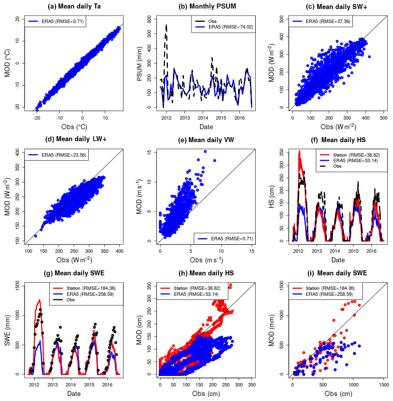
Figure 3Multiyear simulations at the WFJ station (WY2012–2017) in order to show baseline results for the modelling scheme. Panels (a)–(e) assess the downscaling scheme by showing downscaled ERA5 data (ERA5) compared to station measurements (Obs). Panels (f)–(i) assess the simulation of target variables, SWE and HS, in both time series and scatter plots. Here, ERA5 is a simulation driven either by downscaled ERA5 (ERA5) or directly by station measurements (Station). Obs are SWE and HS measurements made at the station. WY2012 is a clear outlier in poor performing ERA5 as shown by cumulative precipitation errors and in the HS and SWE time series. The HS and SWE scatter plots also show this low performance in high values attributed to WY2012. Additionally, ERA5-simulated HS is increasingly biased with depth as errors accumulate over the season to maximum depth values. The same pattern is evident for SWE. It is worth noting that these plots are useful in differentiating sources of error. Obs minus Station approximates model error, whereas Station minus ERA5 approximates the forcing error.

Figure 4DA run at the Truebsee GCOS station, Engelberg. Panel (a) shows the assimilation step with the assimilated fSCA observations represented by black crosses. The shading and solid lines show the 90th percentile range and median of the prior (red) and posterior (blue) estimates. Panel (b) shows the target variable validation (SWE in this case). Posterior/prior are denoted in the same way. Black triangles indicate the measurements used for the validation.
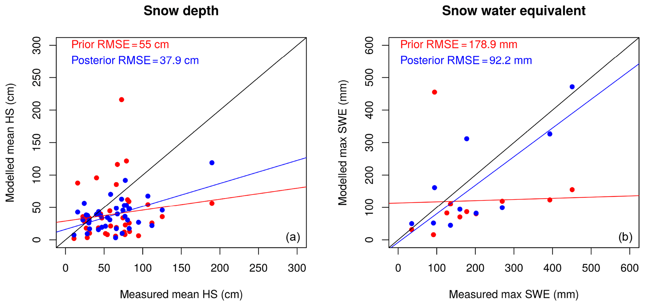
Figure 5Simulated snow depth at the IMIS stations (HS) and snow water equivalent at the GCOS stations (SWE) for both the prior (red) and posterior median (blue) compared to the observation mean. The mean is computed from all values over the entire WY2016. The posterior estimate is markedly improved in both variables. Regression lines compare the fit of the posterior and prior estimates with respect to observations against the 1 : 1 line.
5.2 Point DA
In this experiment we compare the prior and (single-pixel) posterior HS and SWE for WY2016 to the measured values at the respective stations. An example at Truebsee GCOS station (Engelberg) is shown in Fig. 4. This figure demonstrates the effect that the assimilation has not only on the fSCA (which is assimilated), but also on estimates of the other state variables (in this case SWE) which get closer to independent observations. Here one can clearly see how the posterior estimate of SWE (blue shading) is constrained by the assimilation, and the posterior median (blue line) is much closer to validation SWE observations than the prior (red line). We then scaled this up to nine ERA5 grid boxes that span the Swiss Alps and contain 11 GCOS SWE stations. Additionally each box contains multiple IMIS stations measuring HS, which we also looked at in the interest of obtaining more validation data. Significant improvements in the posterior were seen in the estimation of both variables (Fig. 5). We found that the improvement in the SWE was greater than that in the HS. We hypothesize that this is due to representation of snow densities in the snow model. However, the improved representation of the snowpack mass balance as shown by improved SWE estimates is the main variable of interest in our approach. Stations where DA performed worse than the prior can be attributed to poorly characterized melt seasons, lack of MODIS retrievals and/or the MODIS retrievals not being representative at the scale of the observations (cf. Sect. 6).
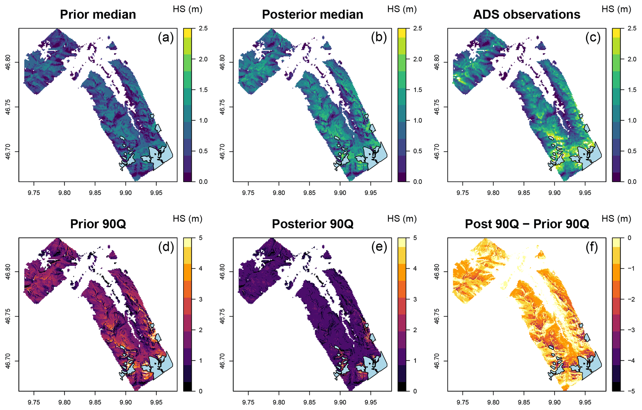
Figure 6(a–c) Prior/posterior median and observations from ADS sensor flights in the Davos region on 14 April 2014 (see Fig. 2 for location). (d–f) Uncertainty represented by the 90th percentile range of the ensemble and the reduction in the uncertainty in the posterior. The glacier mask is shown in blue. The posterior median is improved with respect to the observations, and the uncertainty is reduced by the DA scheme.
5.3 Spatially distributed DA
We evaluated the performance of the method in improving the spatial patterns and absolute quantities over large areas using data from an airborne digital sensor which has been used to generate high-resolution surfaces of HS in WY2012, WY2013 and WY2014 (Fig. 6, WY2014 only). Both WY2012 and WY2014 show marked improvement in all spatial statistical measures including the mean value, the standard deviation (indicating increased variation) and error statistics such as the RMSE and bias. WY2013 shows little improvement. We would expect a better performance for SWE than for HS due to the previously mentioned issues with the modelled snow density (see Sect. 5.2 and Fig. 5). Figure 6 shows how the 90th percentile range is constrained by the analysis going from the prior to the posterior. Figure 7 shows probability density distributions for observations, prior and posterior in WY2014. The shape and moments, such as the mean, more closely match the observations in the posterior distribution. However, the method fails to capture the very highest accumulations in the distribution (>2.5 m), possibly due to the averaging effects of generalizing weights to TopoSUB clusters.
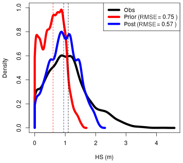
Figure 7Density distribution plots for HS Obs, prior and posterior within the ADS footprint for 14 April 2014 (see Fig. 6). The observed distribution is better captured by the posterior. Dashed lines give the respective mean values.
5.3.1 Interannual validity of weights
We tested the ability of weights obtained in a given hydrological year to improve results in a different year. We did this by looking at statistics on the Dischma Basin via a cross-validation exercise where each year was forced with results from the 2 other years (WY2012, WY2013 and WY2014). Posteriors forced by the weights of other years improved performance over priors in all cases (Fig. 8). This suggests that the DA method here also works to correct errors that are consistent from year to year. This could be related to spatial patterns of melt, which is a consistent bias in the forcing or errors in the model itself. This is an interesting result that suggests that while this method is primarily a post-processing method, it could be used to improve now/forecasts by using previous year's weights. Additionally an analogue approach could be used to find the years of best fit to the current season in order to select weight sets (Kolberg and Gottschalk, 2010).
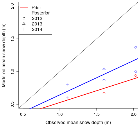
Figure 8Interannual validity of weights generated by the DA scheme. Modelled versus observed mean snow depth averaged over the entire ADS zone on ADS acquisition dates WY2012, WY2013 and WY2014 are shown. Posteriors (blue) are generated using the weights of the other 2 years and are compared to the prior (red). For example, posteriors of WY2012 are generated using weights of WY2013 and WY2014.
5.3.2 Large-scale application: seasonal variability
December 2016 was an extremely snow-poor month and start to the winter season. Many ski areas throughout the Alps could not open until late January due to lack of snow. We compare this to December 2011 which was relatively snow rich with above average precipitation and average temperatures for the month (cf. https://www.meteoswiss.admin.ch/home/climate/swiss-climate-in-detail/monthly-and-annual-maps.html, last access: 9 November 2019). Specifically, we investigated how open-loop runs in two contrasting seasons compared to observed spatial patterns of fSCA from MODIS and SLF reports dated 22 December of the respective year (Fig. 9). The model was found to compare well with both spatial patterns of fSCA and SLF snow depth maps, which are operational products created by interpolating station data constrained by the advanced very-high-resolution radiometer (AVHRR)-observed snow extent. Both fSCA and HS show snow-free zones deep into Alpine valleys during December 2016, and the absence of snow over the northern regions and Jura Mountains. The red box indicates the domain of the DA runs for these seasons shown in Fig. 10.
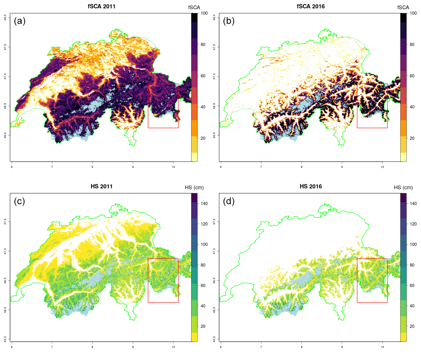
Figure 9Mean December high-resolution (30 m) large area HS simulations (open loop) in two contrasting seasons (c, d) compared to the observed spatial patterns of fSCA from mean December MODIS retrievals (a, b). Modelled HS compares well to the spatial pattern of fSCA. December 2016 was an extremely dry start to the season with many ski resorts unable to open until late January. Both observed fSCA and modelled HS show snow reflecting this fact, with snow-free zones deep into Alpine valleys. The red box indicates the domain of the DA runs for theses seasons shown in Fig. 11. The glacier mask is shown using light blue.
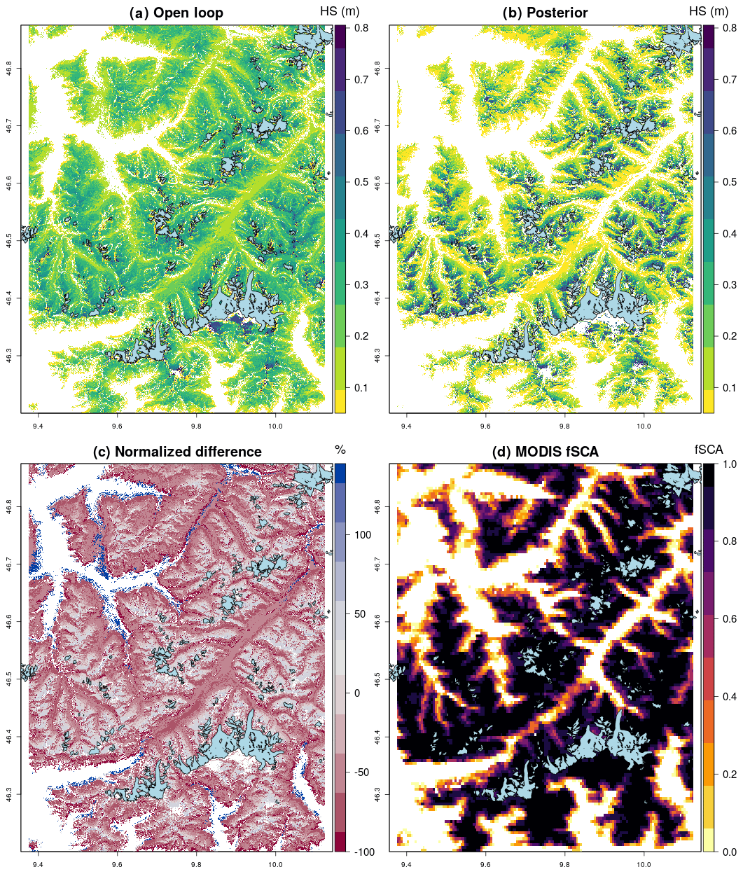
Figure 10The mean HS for December 2016, showing the (a) open loop compared to (b) posterior. (c) The difference plot shows how DA has reduced the low-elevation snow height relatively more than the high-elevation snow height. Variability has been increased. Snow-free valley bottoms in panel (b) show an improved match to (d) MODIS Obs and that the increased spatial variability is realistic.
Next we zoomed in and compared spatial patterns of HS between the deterministic open-loop and posterior run; this demonstrated that DA increased elevation gradients of variability by reducing HS in valley bottoms and increasing it on higher slopes. Thus, DA, as mentioned previously, has the effect of increasing variability in the snow cover distribution. Snow cover extent estimation is also improved by DA with increased snow-free areas in valley bottoms showing an improved fit to MODIS observations.
5.4 Coarse-scale DA
Aggregated series of observed and modelled fSCA are computed at the ERA grid level. This could equally be a hydrological unit such as a basin. The main idea is to correct grid-level biases in the forcing only. If we assume this is the main source of uncertainty, especially with a view to correcting large-scale biases, this is an effective method to apply at the scale of meteorological reanalysis. Data from WFJ are used to illustrate this point. Figure 11 shows two contrasting snow seasons – WY2012 (high) and WY2014 (low) – where mean snow depths and SWE differed by a factor of 2, as recorded at WFJ (Fig. 3). We compare the total ERA5 precipitation (PSUM) over the winter period January–April 2014 (401 mm) and compare it to totals recorded over the same period at the WFJ station (350 mm), ERA5 captures WFJ totals well. It should be added that there is some elevation difference between the ERA5 grid (2024 m a.s.l.) and the WFJ station (2560 m a.s.l.). However, in WY2012 we see quite a different story. The ERA5 grid gives us slightly higher PSUM values of 440 mm, whereas the measured PSUM was almost double this at 826 mm. Figure 11 shows how grid-level biases in the driving forcing from ERA5 have been successfully decreased in WY2012 resulting in increased SWE totals, whereas in WY2014 where ERA5 performance was much better (cf. Fig. 3), DA has had a negligible effect. This simple approach is an extremely cost-effective method of assimilating slope-scale sub-grid information (in this case fSCA) to correct coarse grid-scale forcings (ERA5). It is additionally generic enough that it could be used with various other sub-grid observations, such as soil moisture, to improve grid-level responses.
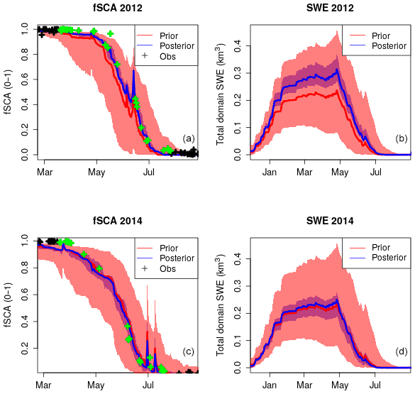
Figure 11Assimilation of fSCA at the grid level which targets bias in grid-level forcing. Two contrasting seasons, WY2012 (a, b) and WY2014 (c, d), are shown. The shading and solid lines show the 90th percentile range and median of the prior (red) and posterior (blue) estimates respectively. Assimilated observations are indicated in green. Grid-level biases in WY2012 are compensated for by DA. Grid-level forcing was much more accurate in WY2014 and the resulting effect of DA was negligible.
In the following discussion some emphasis is placed on sources of uncertainty arising due to generally unknown errors in both the model, observations and forcing. These errors can be systematic (bias) or random as well as errors of representativeness (e.g. Lahoz and Schneider, 2014). Accounting for the uncertainty that results from these errors is an important component of any DA framework.
6.1 Sources of error
6.1.1 Forcing bias
In this work, we encounter two forms of bias in the forcing. The first of these is (i) grid-level inputs or bias in the forcing ERA5 reanalysis. This may exist due to e.g. a bias in assimilated observations (SYNOP stations tend to be in valley bottoms) or errors, omissions and parameterizations in the atmospheric model itself. How different is the forcing from observed grid-averaged conditions? Of course this is a very difficult question to answer. Although with products such as precipitation radars such comparison of modelled and measured grid integrated precipitation may be possible. The second (ii) is error (random or bias) in the downscaling routines or disaggregation of the forcing at the sub-grid level. Do we get gradients along topographic correct? These sources of error could well be reinforcing or indeed cancelling, as they can be independent sources of error. In the approach of spatial DA we address both systematic and random error in the forcing, but with an emphasis on the former. There is no 2-D redistribution in terms of longitude and latitude position of a grid box. All members of a cluster are equally perturbed and clusters do not have x,y coordinates. In point DA, again both sources are addressed but with a stronger focus on (ii) as the data assimilation is carried out at the MODIS pixel level and, therefore, redistributes precipitation not only with topographic parameters but also in a spatial x,y sense. In grid DA we only address (i) which could be a useful approach with respect to differentiating and quantifying sources of bias as well as simply and robustly addressing the question of grid-level bias.
6.1.2 Model error
We do not focus on structural errors in the forward model as this was not the subject of this study; furthermore, the methods are designed to be quite independent of model type. It is worth noting that the majority of the results in this paper have focused on HS due to higher data availability. However, Fig. 5 shows that results are significantly better for SWE, possibly due to errors in the model densification parameterizations. Therefore, this is reassuring as HS results can be interpreted as conservative; thus, if we were able to validate more extensively against spatial distributed SWE measurements, we would likely see improved results.
6.1.3 Melt period definition
An important feature to mention that is not often addressed by DA studies (Morzfeld et al., 2018, is a nice exception) is the sensitivity of data assimilation methods to the observations chosen for assimilation. In the case of fSCA assimilations a melt period is defined as this is when the observations provide information about the snow depletion curve (e.g. Aalstad et al., 2018). We identify the end of the snowpack as the first day that the fSCA values reach zero. There may be short increases in fSCA after this date but these will generally be late spring/summer snowfalls that are transient and melt rapidly. However, this date is the first available zero fSCA observation which does not necessarily equate to the exact date that the snowpack melts out as there can be a lack of observations due to cloud cover. Therefore, this should be considered as a source of potential bias in the system. We then found that a fixed window of 30 d prior to this date was a simple and robust way of defining the melt period. We trialled other methods of automatically defining the end of the “complete snow cover” period but we did not find a way to do this that could work robustly over several hundred thousand MODIS pixels. Additionally, the MODIS products are prone to various sources of error, as discussed below in Sect. 6.1.5, and this adds to the difficulty in defining a robust, general algorithm that defines the start of the melt period. As mentioned above, this is a little discussed topic but, due to the sensitivity of final results to the chosen method, it would certainly benefit from further research efforts.
6.1.4 Scale issues in assimilation
The scale difference between validation data (station or snow profile) and fSCA retrievals from MODIS creates several issues. In this study many of the sites are in valley bottoms so they are accessible on a regular basis. However, this creates a bias caused by how representative the point measurement of the larger MODIS pixel footprint is. In Alpine valley bottoms there tends to be a lot of infrastructure, housing and rivers, which will tend to be snow free earlier (or never snow covered) compared with a station site that is well protected from interference allowing the natural accumulation of snowfall. Therefore, the MODIS footprint will tend to be observed as “snow free” earlier than the validation point. In addition features such as a rivers, road clearance and urban heat islands are not considered in the modelling and will generate bias in the data assimilation. Thus, the most reliable sites for data assimilation, or actually we should say for validating the method, are at high elevations away from effects due to human activity or infrastructure that are not considered in the model. Figure 12 gives an example of a point-scale DA failure that is not due to the DA algorithm (this has worked well), but stems from the representativeness of the fSCA retrievals. The posterior has correctly been pulled in the direction of what has been detected to be the main melt period (red dots), erroneous snowfalls during late spring/early summer are ignored as expected and the end of the winter snowpack (as detected by the fSCA retrievals) has been correctly identified at the beginning of April. However, this site is in the middle of Zermatt town and the MODIS pixel will likely contain a signal from urban effects unaccounted for by the model.
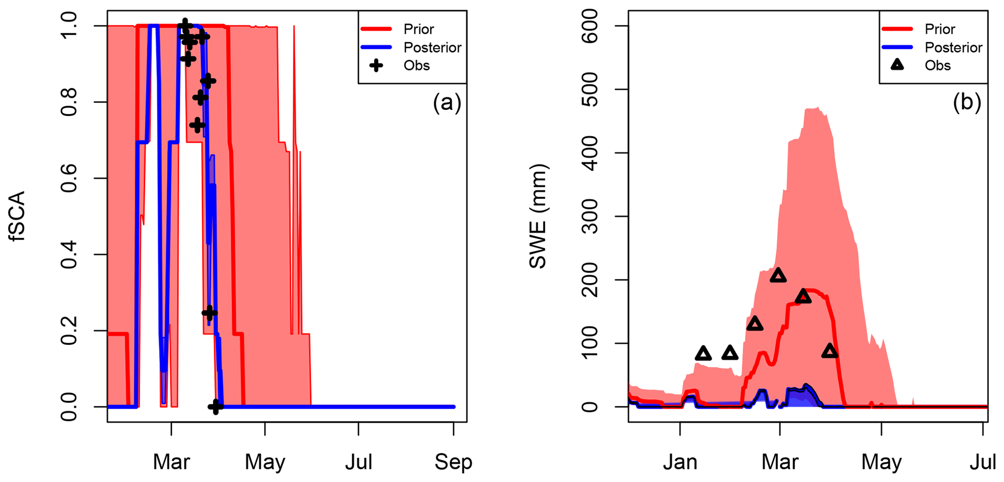
Figure 12An example of poor performance due to the non-representative fSCA retrievals. The posterior has been correctly pulled back to the observed depletion curve. However, it is likely that the depletion curve does not represent the validation station well due to urban effects.
6.1.5 Observational errors
In addition to the scale issues, there are actual errors and cloud-induced data gaps in the MODIS retrievals. This could be incorrectly classified clouds (as snow or vice-versa) or uncertainty in the empirical fSCA algorithm. In addition, the method can also suffer from a lack of observations due to persistent cloudiness at key points in the melt period which will create uncertainties during DA. It may be worthwhile considering fSCA retrievals from different higher-resolution satellite constellations such as Landsat (30 m resolution) and Sentinel-2 (20 m resolution). This would increase the chance of obtaining cloud-free scenes as well as reduce representativeness errors even at resolutions as high as 100 m. Furthermore, the aggregation of higher-resolution retrievals would lead to a reduction of random error. The effective MODIS footprint of individual pixels can be quite variable and differs markedly from the nominal 500 m pixel resolution when the view angle deviates from nadir (Dozier et al., 2008). Therefore, even for gridded applications, there is a considerable representativeness error in the MODIS fSCA. A final, important limitation of the scheme is the lack of reliable fSCA retrievals in forested areas, which applies to any optical sensor (e.g. as mentioned in the description of the ADS data).
6.2 Applications
Using the methods described in this paper, a range of processing pipelines can be built to address a wide array of both research and operational problems. Specific strengths of the approach are as follows:
-
there is slope-scale forcing (climate, reanalysis, forecast) globally;
-
the approach explicitly includes the effects of high-resolution topography on surface–atmosphere interactions;
-
it is an efficient method to make large ensemble simulations feasible;
-
there is data assimilation to correct bias in forcing and quantify uncertainty.
Perhaps most importantly this approach allows applications to be built in remote regions where dense observation networks do not exist, such as High Mountain Asia or parts of North America. These capabilities allow for operational applications such as large area mass movement assessments related to the dynamics of surface and subsurface processes. Driving the system with NWP (forecast) data would allow nowcasting/forecasting applications to be set up with a suitable assimilation framework such as the ensemble Kalman filter (EnKF). While the assimilation of fSCA would be less informative in a sequential method (such as the EnKF), ensemble simulations would still provide a useful quantification of uncertainty.
Transient climate change studies using a combination of reanalysis and climate model data (e.g. CMIP5) would be a valuable research application based on this approach, for example quantifying dynamics of permafrost extent over large areas according to a range of scenarios and models or generating a regional snowpack reanalysis product with projected future changes.
An important operational application and currently a great humanitarian need in many remote regions in Asia (e.g. Afghanistan/Tajikistan) could be an operational avalanche forecast based on a snowpack model (e.g. SNOWPACK, CROCUS), driven by an NWP ensemble to generate a large area probabilistic forecast where few ground stations exist. This would be a relatively cost-effective system to deploy and give first-order hazard assessment where none currently exists.
6.3 Further work
For the moderate (MODIS-like) resolution satellites, we hope that products will emerge from Sentinel-3 and VIIRS to prolong and expand the MODIS record. For high-resolution sensors, there is a strong need for operational products that ideally combine available and emerging sources such as Landsat 8 and Sentinel-2. The French inter-agency initiative THEIA Land Data Centre is starting to produce Sentinel-2-based snow cover products (Gascoin et al., 2019), which – at both high temporal and spatial resolution – will likely prove to be a great product for data assimilation work. Additionally, improved cloud masks are needed as misclassified clouds are potential and significant sources of error in the framework. Both overly strict and overly relaxed cloud masking is problematic, the former leads to valid and potentially important retrievals being discarded, whereas the latter corrupts the signal that we are trying to assimilate (the actual snow cover depletion).
For additional datasets (other than fSCA), land surface temperature can be retrieved from both MODIS and Landsat and provide a means to constrain uncertainty in the surface energy balance. However, the current MODIS products are coarse at 1 km and, therefore, not ideal for mountain regions.
For additional datasets (other than fSCA), land surface temperature (LST) can be retrieved from both MODIS and Landsat and provide a means to constrain uncertainty in the surface energy balance. However, the current MODIS LST products are coarse at 1 km with respect to the expected heterogeneity of LST in mountain regions (Gubler et al., 2011). Snowmelt status (i.e. binary melting/not melting) from synthetic aperture radar (SAR) e.g. Sentinel-1 has the potential to constrain uncertainty in the fSCA during cloudy periods. There is also potential from ICESat-2 which could provide a way to constrain snow depth directly (Treichler and Kääb, 2017).
Assimilation of sparse point data could be an important extension of this work to provide means to assimilate data sources such as ICESat-2 but could also be used to improve TopoSCALE by assimilating point data (stations) to improve the downscaling of reanalysis data. This could be interesting as TopoSCALE performs most poorly is in valleys, where surface effects are poorly represented by the atmospheric model, and this is precisely where stations tend to be most abundant globally. For real-time applications in remote regions, extending the method to assimilate sparse observations is important as fSCA is known to have limited value in sequential (i.e real-time) data assimilation. We have shown that there is some interannual validity of results in our limited test case, suggesting that systematic biases relevant to real-time applications could be addressed through reanalysis. Additionally, creating a long-term library of “best possible” reconstructions/reanalyses and then training an “analogue ensemble” or even a more machine-learning-type approach (like neural nets) could be promising.
In this study we have demonstrated a processing pipeline capable of producing improved land surface simulations at scale in ungauged regions. It consists of downscaling, sub-grid and data assimilation components and uses only globally available datasets for both the model forcing and assimilated observations; therefore, it is suitable for global applications. Specifically we have shown that
-
the use of PBS data assimilation can significantly improve estimates of snowpack at various spatial scales;
-
TopoSUB clustering efficiency gains make large ensemble simulations feasible;
-
the methods can be used to reduce biases both at the coarse atmospheric grid scale and also at scales related to the downscaling routines;
-
the approach is suitable for regional to global applications due to efficiency and data requirements;
-
a flexible set of tools allows various research and operational problems to be addressed where high-resolution surface models are needed in heterogeneous terrain.
We propose this as a suitable method for complex model ensemble runs at scale i.e. large numbers of particles, large spatial areas or long temporal periods. Application areas include any problem where accurate slope-scale forcings are required and surface atmosphere interactions need to be simulated at the slope scale e.g. large area avalanche warning where the snowpack is explicitly simulated or regional-scale hazard assessment of mass movements where the changing ground thermal regime is a risk factor. The tool chain can be flexibly driven by a range of forcings e.g. climate scenario data, reanalysis of past climate, or real-time NWP and drive impact models for a range of domains e.g., hydrology, snow cover, soil stability or permafrost. New developments in multi-platform processing pipelines of high-resolution products from Sentinel-2 and Landsat will further improve the method in terms of representativity and availability of observations.
All code used in this publication is available at https://github.com/joelfiddes/topoMAPP (Fiddes, 2019). The airborne digital sensor data used in this study is freely available at: https://doi.org/10.16904/23 (Vögeli et al., 2016b).
JF wrote the grant proposal for the postdoc SNF project “TopoSAT”. JF and SW designed the study. KA contributed to the implementation of the DA module and multiple aspects of the analysis. JF wrote the paper which was contributed to and edited by all co-authors.
The authors declare that they have no conflict of interest.
We acknowledge the Swiss National Science Foundation (project number P2ZHP2_165435 “TopoSAT: High resolution surface modelling of the Himalayan cryosphere with satellite data assimilation”) and SatPerm (grant no. 239918; Research Council of Norway) for providing funding for this study. We thank all data providers for making their data freely available.
This research has been supported by the Swiss National Science Foundation (project no. P2ZHP2_165435) and the Research Council of Norway (grant no. 239918).
This paper was edited by Carlo De Michele and reviewed by Richard L. H. Essery and Simon Gascoin.
Aalstad, K., Westermann, S., Schuler, T. V., Boike, J., and Bertino, L.: Ensemble-based assimilation of fractional snow-covered area satellite retrievals to estimate the snow distribution at Arctic sites, The Cryosphere, 12, 247–270, https://doi.org/10.5194/tc-12-247-2018, 2018. a, b, c, d, e, f, g, h, i, j
Baldo, E. and Margulis, S. A.: Assessment of a multiresolution snow reanalysis framework: a multidecadal reanalysis case over the upper Yampa River basin, Colorado, Hydrol. Earth Syst. Sci., 22, 3575–3587, https://doi.org/10.5194/hess-22-3575-2018, 2018. a, b
Bertoldi, G., Rigon, R., and Over, T. M.: Impact of watershed geomorphic characteristics on the energy and water budgets, J. Hydrometeorol., 7, 389–403, https://doi.org/10.1175/JHM500.1, 2006. a
Beven, K. and Binley, A.: The Future of Distributed Models: Model Calibration and Uncertainty Prediction, Hydrol. Process., 6, 279–298, https://doi.org/10.1002/hyp.3360060305, 1992. a
Beven, K. J. and Kirkby, M. J.: A physically based, variable contributing area model of basin hydrology/Un modèle à base physique de zone d'appel variable de l'hydrologie du bassin versant, Hydrol. Sci. B., 24, 43–69, 1979. a
Bierkens, M. F. P., Bell, V. A., Burek, P., Chaney, N., Condon, L. E., David, C. H., de Roo, A., Döll, P., Drost, N., Famiglietti, J. S., Flörke, M., Gochis, D. J., Houser, P., Hut, R., Keune, J., Kollet, S., Maxwell, R. M., Reager, J. T., Samaniego, L., Sudicky, E., Sutanudjaja, E. H., van de Giesen, N., Winsemius, H., and Wood, E. F.: Hyper-resolution global hydrological modelling: what is next?, Hydrol. Process., 29, 310–320, 2015. a
Bühler, Y., Marty, M., Egli, L., Veitinger, J., Jonas, T., Thee, P., and Ginzler, C.: Snow depth mapping in high-alpine catchments using digital photogrammetry, The Cryosphere, 9, 229–243, https://doi.org/10.5194/tc-9-229-2015, 2015. a, b, c
Carrassi, A., Bocquet, M., Bertino, L., and Evensen, G.: Data assimilation in the geosciences: An overview of methods, issues, and perspectives, WIRES Clim. Change, 9, e535, https://doi.org/10.1002/wcc.535, 2018. a, b
Dall'Amico, M., Endrizzi, S., Gruber, S., and Rigon, R.: A robust and energy-conserving model of freezing variably-saturated soil, The Cryosphere, 5, 469–484, https://doi.org/10.5194/tc-5-469-2011, 2011. a
De Lannoy, G. J. M., Reichle, R. H., Arsenault, K. R., Houser, P. R., Kumar, S., Verhoest, N. E. C., and Pauwels, V. R. N.: Multiscale assimilation of Advanced Microwave Scanning Radiometer–EOS snow water equivalent and Moderate Resolution Imaging Spectroradiometer snow cover fraction observations in northern Colorado, Water Resour. Res., 48, W01522, https://doi.org/10.1029/2011WR010588, 2012. a, b
Dozier, J., Painter, T. H., Rittger, K., and Frew, J. E.: Time–space continuity of daily maps of fractional snow cover and albedo from MODIS, Adv. Water Resour., 31, 1515–1526, https://doi.org/10.1016/j.advwatres.2008.08.011, 2008. a
Dozier, J., Bair, E. H., and Davis, R. E.: Estimating the spatial distribution of snow water equivalent in the world's mountains, WIRES Water, 3, 461–474, 2016. a, b, c
Durand, Y., Brun, E., Merindol, L., Guyomarc'h, G., Lesaffre, B., and Martin, E.: A meteorological estimation of relevant parameters for snow models, Ann. Glaciol., 18, 65–71, 1993. a
Endrizzi, S.: Snow cover modelling at a local and distributed scale over complex terrain, PhD thesis, Dept. of Civil and Environmental Engineering, University of Trento, Trento, Italy, 2007. a
Endrizzi, S., Gruber, S., Dall'Amico, M., and Rigon, R.: GEOtop 2.0: simulating the combined energy and water balance at and below the land surface accounting for soil freezing, snow cover and terrain effects, Geosci. Model Dev., 7, 2831–2857, https://doi.org/10.5194/gmd-7-2831-2014, 2014. a
Fiddes, J.: TOPOgraphy based Modelling APPlication: TopoMAPP, available at: https://github.com/joelfiddes/topoMAPP, last access: 9 November 2019. a
Fiddes, J. and Gruber, S.: TopoSUB: a tool for efficient large area numerical modelling in complex topography at sub-grid scales, Geosci. Model Dev., 5, 1245–1257, https://doi.org/10.5194/gmd-5-1245-2012, 2012. a, b, c, d
Fiddes, J. and Gruber, S.: TopoSCALE v.1.0: downscaling gridded climate data in complex terrain, Geosci. Model Dev., 7, 387–405, https://doi.org/10.5194/gmd-7-387-2014, 2014. a, b, c, d
Fiddes, J., Endrizzi, S., and Gruber, S.: Large-area land surface simulations in heterogeneous terrain driven by global data sets: application to mountain permafrost, The Cryosphere, 9, 411–426, https://doi.org/10.5194/tc-9-411-2015, 2015. a, b, c
Gascoin, S., Grizonnet, M., Bouchet, M., Salgues, G., and Hagolle, O.: Theia Snow collection: high-resolution operational snow cover maps from Sentinel-2 and Landsat-8 data, Earth Syst. Sci. Data, 11, 493–514, https://doi.org/10.5194/essd-11-493-2019, 2019. a
Girotto, M., Margulis, S. A., and Durand, M.: Probabilistic SWE reanalysis as a generalization of deterministic SWE reconstruction techniques, Hydrol. Process., 28, 3875–3895, 2014. a, b
Griessinger, N., Seibert, J., Magnusson, J., and Jonas, T.: Assessing the benefit of snow data assimilation for runoff modeling in Alpine catchments, Hydrol. Earth Syst. Sci., 20, 3895–3905, https://doi.org/10.5194/hess-20-3895-2016, 2016. a
Gruber, S. and Haeberli, W.: Permafrost in steep bedrock slopes and its temperature‐related destabilization following climate change, J. Geophys. Res.-Earth, 112, F02S18, https://doi.org/10.1029/2006JF000547, 2007. a
Gubler, S., Fiddes, J., Keller, M., and Gruber, S.: Scale-dependent measurement and analysis of ground surface temperature variability in alpine terrain, The Cryosphere, 5, 431–443, https://doi.org/10.5194/tc-5-431-2011, 2011. a
Gubler, S., Gruber, S., and Purves, R. S.: Uncertainties of parameterized surface downward clear-sky shortwave and all-sky longwave radiation., Atmos. Chem. Phys., 12, 5077–5098, https://doi.org/10.5194/acp-12-5077-2012, 2012. a, b
Hall, D. K. and Riggs, G. A.: MODIS/Terra Snow Cover Daily L3 Global 500m Grid, Version 6, Tile h18v01, NASA National Snow and Ice Data Center Distributed Active Archive Center, Boulder, Colorado USA, https://doi.org/10.5067/MODIS/MOD10A1.006, 2016a. a
Hall, D. K. and Riggs, G. A.: MODIS/Aqua Snow Cover Daily L3 Global 500m Grid, Version 6, Tile h18v01, NASA National Snow and Ice Data Center Distributed Active Archive Center, Boulder, Colorado USA, https://doi.org/10.5067/MODIS/MYD10A1.006, 2016b. a
Kolberg, S. and Gottschalk, L.: Interannual stability of grid cell snow depletion curves as estimated from MODIS images, Water Resour. Res., 46, W11555, https://doi.org/10.1029/2008WR007617, 2010. a
Lahoz, W. A. and Schneider, P.: Data assimilation: making sense of Earth Observation, Front. Environ. Sci., 2, 16, https://doi.org/10.3389/fenvs.2014.00016, 2014. a, b
Liston, G. E.: Representing subgrid snow cover heterogeneities in regional and global models, J. Climate, 17, 1381–1397, 2004. a
Liu, Y., Weerts, A. H., Clark, M., Hendricks Franssen, H.-J., Kumar, S., Moradkhani, H., Seo, D.-J., Schwanenberg, D., Smith, P., van Dijk, A. I. J. M., van Velzen, N., He, M., Lee, H., Noh, S. J., Rakovec, O., and Restrepo, P.: Advancing data assimilation in operational hydrologic forecasting: progresses, challenges, and emerging opportunities, Hydrol. Earth Syst. Sci., 16, 3863–3887, https://doi.org/10.5194/hess-16-3863-2012, 2012. a, b
Magnusson, J., Winstral, A., Stordal, A. S., Essery, R., and Jonas, T.: Improving physically based snow simulations by assimilating snow depths using the particle filter, Water Resour. Res., 53, 1125–1143, 2017. a
Mankin, J. S., Viviroli, D., Singh, D., Hoekstra, A. Y., and Diffenbaugh, N. S.: The potential for snow to supply human water demand in the present and future, Environ. Res. Lett., 10, 114016, https://doi.org/10.1088/1748-9326/10/11/114016, 2015. a
Margulis, S. A., Girotto, M., Cortés, G., and Durand, M.: A Particle Batch Smoother Approach to Snow Water Equivalent Estimation, J. Hydrometeorol., 16, 1752–1772, 2015. a, b, c, d, e, f, g
Martinec, J. and Rango, A.: Areal Distribution of Snow Water Equivalent Evaluated by Snow Cover Monitoring, Water Resour. Res., 17, 1480–1488, https://doi.org/10.1029/WR017i005p01480, 1981. a, b
Marty, C.: GCOS SWE data from 11 stations in Switzerland, WSL Institute for Snow and Avalanche Research SLF, https://doi.org/10.16904/15, 2017. a
Mascaro, G., Vivoni, E. R., and Méndez-Barroso, L. A.: Hyperresolution hydrologic modeling in a regional watershed and its interpretation using empirical orthogonal functions, Adv. Water Resour., 83, 190–206, 2015. a
Masson, T., Dumont, M., Dalla Mura, M., Sirguey, P., Gascoin, S., Dedieu, J. P., and Chanussot, J.: An Assessment of Existing Methodologies to Retrieve Snow Cover Fraction from MODIS Data, Remote Sensing, 10, 619, https://doi.org/10.3390/rs10040619, 2018. a
Morzfeld, M., Adams, J., Lunderman, S., and Orozco, R.: Feature-based data assimilation in geophysics, Nonlin. Processes Geophys., 25, 355–374, https://doi.org/10.5194/npg-25-355-2018, 2018. a
Navari, M., Margulis, S. A., Bateni, S. M., Tedesco, M., Alexander, P., and Fettweis, X.: Feasibility of improving a priori regional climate model estimates of Greenland ice sheet surface mass loss through assimilation of measured ice surface temperatures, The Cryosphere, 10, 103–120, https://doi.org/10.5194/tc-10-103-2016, 2016. a
Painter, T. H., Rittger, K., McKenzie, C., Slaughter, P., Davis, R. E., and Dozier, J.: Retrieval of subpixel snow covered area, grain size, and albedo from MODIS, Remote Sens. Environ., 113, 868–879, https://doi.org/10.1016/j.rse.2009.01.001, 2009. a
Raleigh, M. S., Lundquist, J. D., and Clark, M. P.: Exploring the impact of forcing error characteristics on physically based snow simulations within a global sensitivity analysis framework, Hydrol. Earth Syst. Sci., 19, 3153–3179, https://doi.org/10.5194/hess-19-3153-2015, 2015. a
Raup, B., Racoviteanu, A., Khalsa, S. J. S., Helm, C., Armstrong, R., and Arnaud, Y.: The GLIMS geospatial glacier database: A new tool for studying glacier change, Global Planet. Change, 56, 101–110, 2007. a
Reichle, R. H., Koster, R. D., Liu, P., Mahanama, S. P. P., Njoku, E. G., and Owe, M.: Comparison and assimilation of global soil moisture retrievals from the Advanced Microwave Scanning Radiometer for the Earth Observing System (AMSR-E) and the Scanning Multichannel Microwave Radiometer (SMMR), J. Geophys. Res., 112, 1697, https://doi.org/10.1029/2006JD008033, 2007. a, b
Rigon, R., Bertoldi, G., and Over, T. M.: GEOtop: A Distributed Hydrological Model with Coupled Water and Energy Budgets, J. Hydrometeorol., 7, 371–388, https://doi.org/10.1175/JHM497.1, 2006. a
Salomonson, V. V. and Appel, I.: Development of the Aqua MODIS NDSI Fractional Snow Cover Algorithm and Validation Results, IEEE T. G. Remote, 44, 1747–1756, https://doi.org/10.1109/TGRS.2006.876029, 2006. a
Shur, Y. L. and Jorgenson, M. T.: Patterns of permafrost formation and degradation in relation to climate and ecosystems, Permafrost Periglac., 18, 7–19, 2007. a
Slater, A. G., Barrett, A. P., Clark, M. P., Lundquist, J. D., and Raleigh, M. S.: Uncertainty in seasonal snow reconstruction: Relative impacts of model forcing and image availability, Adv. Water Resour., 55, 165–177, https://doi.org/10.1016/j.advwatres.2012.07.006, 2013. a
Thirel, G., Salamon, P., Burek, P., and Kalas, M.: Assimilation of MODIS Snow Cover Area Data in a Distributed Hydrological Model Using the Particle Filter, Remote Sensing, 5, 5825–5850, 2013. a
Treichler, D. and Kääb, A.: Snow depth from ICESat laser altimetry – A test study in southern Norway, Remote Sens. Environ., 191, 389–401, https://doi.org/10.1016/j.rse.2017.01.022, 2017. a
Tucker, G. E., Lancaster, S. T., Gasparini, N. M., Bras, R. L., and Rybarczyk, S. M.: An object-oriented framework for distributed hydrologic and geomorphic modeling using triangulated irregular networks, Comput. Geosci., 27, 959–973, 2001. a
Van Leeuwen, P. J.: Particle Filtering in Geophysical Systems, Mon. Weather Rev., 137, 4089–4114, https://doi.org/10.1175/2009MWR2835.1, 2009. a, b, c
Van Leeuwen, P. J. and Evensen, G.: Data assimilation and inverse methods in terms of a probabilistic formulation, Mon. Weather Rev., 124, 2898–2913, https://doi.org/10.1175/1520-0493(1996)124<2898:DAAIMI>2.0.CO;2, 1996. a, b, c
Vögeli, C., Lehning, M., Wever, N., and Bavay, M.: Scaling Precipitation Input to Spatially Distributed Hydrological Models by Measured Snow Distribution, Front. Earth Sci., 4, 108, https://doi.org/10.3389/feart.2016.00108, 2016a. a, b
Vögeli, C., Lehning, M., and Bavay, M.: Precipitation Scaling Data Set (Vögeli et al., Frontiers), Frontiers in Earth Science, https://doi.org/10.16904/23, 2016b. a, b
Wood, E. F., Roundy, J. K., Troy, T. J., van Beek, L. P. H., Bierkens, M. F. P., Blyth, E., de Roo, A., Döll, P., Ek, M., Famiglietti, J., Gochis, D., van de Giesen, N., Houser, P., Jaffé, P. R., Kollet, S., Lehner, B., Lettenmaier, D. P., Peters-Lidard, C., Sivapalan, M., Sheffield, J., Wade, A., and Whitehead, P.: Hyperresolution global land surface modeling: Meeting a grand challenge for monitoring Earth's terrestrial water, Water Resour. Res., 47, 1–10, 2011. a, b
Zhang, T.: Influence of the seasonal snow cover on the ground thermal regime: An overview, Rev. Geophys., 43, RG4002, https://doi.org/10.1029/2004RG000157, 2005. a