Integrating multiple satellite observations into a coherent dataset to monitor the full water cycle – application to the Mediterranean region

The Mediterranean region is one of the climate hotspots where the climate change impacts are both pronounced and documented. The HyMeX (Hydrometeorological Mediterranean eXperiment) aims to improve our understanding of the water cycle from the meteorological to climate scales. However, monitoring the water cycle with Earth observations (EO) is still a challenge: EO products are multiple, and their utility is degraded by large uncertainties and incoherences among the products. Over the Mediterranean region, these difficulties are exacerbated by the coastal/mountainous regions and the small size of the hydrological basins. Therefore, merging/integration techniques have been developed to reduce these issues. We introduce here an improved methodology that closes not only the terrestrial but also the atmospheric and ocean budgets. The new scheme allows us to impose a spatial and temporal multi-scale budget closure constraint. A new approach is also proposed to downscale the results from the basin to pixel scales (at the resolution of 0.25^∘). The provided Mediterranean WC budget is, for the first time, based mostly on observations such as the GRACE water storage or the netflow at the Gibraltar Strait. The integrated dataset is in better agreement with in situ measurements, and we are now able to estimate the Bosporus Strait annual mean netflow.

1 Introduction

The Mediterranean region is one of the main climate change hotspots (IPCC, 2014): its sensitivity to global change is high and its evolution remains uncertain. Its role in the evolution of the global ocean (i.e., mainly salinization and warming), as well as the socio-economic consequences it has for surrounding countries, stress the need for monitoring its water resource. Analyzing the water cycle (WC) and the exchanges among its terrestrial, atmospheric and oceanic branches is critical for estimating the availability of the water in the Mediterranean region. Most previous studies use model outputs or reanalysis (Mariotti et al., 2002; Sanchez-Gomez et al., 2011), and in situ data networks are too sparse and irregular. A recent paper (Jordà et al., 2017) reviewed the literature on the analysis and quantification of the Mediterranean water budget using observation, model outputs and reanalyses. The WC components are estimated, but their uncertainties remain high. Recommendations are made to increase our use of Earth observations (EO) data, in a coordinated way. EO allow for the monitoring of the WC over long time records, in particular in regions with a low number of in situ stations. But the use of EO data for WC monitoring remains a challenge due to (1) the multiplicity of datasets for the same geophysical parameter, (2) the EO uncertainties (systematic and random errors), and (3) the inconsistency between datasets (for the same component or among the components of the WC). In Pellet et al. (2017), EO are used to monitor the WC over the Mediterranean region: it is shown that the WC budget is not closed and that some integration technique should be used to optimize them.

Several approaches have been considered in order to optimize EO datasets at the global scale, for the WC analysis. The features of some “integration” methods presented in the following are synthesized in Table 1.

The “Princeton” approach – Pan and Wood (2006) presented first a work in which they aimed to close the water balance using EO products. In this work, EO datasets such as precipitation were assimilated into a land surface model (the Variable Infiltration Capacity, VIC) using the combination of a Kalman filter and a closure constraint (see Table 1). The resulting “analysis” dataset is not a pure EO product since the VIC model is largely used. In fact, the authors show that the Kalman filtering plus the closure constraint is equivalent to a traditional Kalman filtering, and then to the application of an independent post-filtering that constrains the closure (De Geeter et al., 1997; Simon and Chia, 2002; Aires, 2014). This post-filtering acts by redistributing the budget residuals within each water component based on the uncertainties of each EO source. Several papers have been published based on this approach (Troy and Wood, 2009; McCabe et al., 2008; Sahoo et al., 2011; Troy et al., 2011; Pan et al., 2012). For instance, in Sheffield et al. (2009), two different precipitation datasets were used over the Mississippi basin. Evapotranspiration was calculated using a revised Penman–Monteith formulation and changes in water storage were estimated from GRACE. For comparison, land surface model outputs, reanalyses data and in situ discharge measurements were used too. The authors concluded that a positive bias of the precipitation datasets leads to an overestimation of the discharge component when the estimation relies on EO data. Meanwhile, the land surface model shows a high degree of agreement with in situ data. The analysis also highlights the importance of error characterization in the individual WC components. Yilmaz et al. (2011) relaxed the closure constraint during the assimilation. This is an important feature because tight closure constraint can result in high-frequency oscillations in the resulting combined dataset. A large constraint is used in our approach (see Table 1).

The NASA-NEWS project – the project aims at a better characterization of the WC using EO data. The first step was to improve the coherency of the satellite retrievals, and then to gather the EO dataset and calibrate them. Some information about the uncertainties of the EO datasets was gathered from the data producers, but this information cannot be straightforwardly used further in the integration process since its evaluation is not homogeneous but product-dependent. The WC budget can be closed using the satellite datasets (Rodell et al., 2015). However, this closure is obtained at the global and annual scales only, and residuals are still significant at regional and monthly scales. Rodell et al. (2015) then use interpolation for a monthly closure. Closing the budget at the global scale was a first step, and closure must now be obtained at finer spatial and temporal scales to monitor more precisely the distribution of the water components as the EO data are designed to do. In Rodell et al. (2015), the storage terms (e.g., groundwater storage) had no significant change when considering annual and global means. This hypothesis was then used at the monthly scale with an optimized interpolation scheme to relax the storage change at the monthly scale. This approach translates into a quadratic quality criterion where storage and fluxes terms are minimized for annual means, at the global scale (see Table 1). One interesting feature in this approach is that both the water (Rodell et al., 2015) and energy (L'Ecuyer et al., 2015) cycles were considered simultaneously in the assimilation, taking into account the physical link between the two cycles through the latent heat flux.

Pan and Wood (2006)Rodell et al. (2015)Aires (2014)Munier et al. (2014)Sahoo et al. (2011)Pan et al. (2012)L'Ecuyer et al. (2015)Munier and Aires (2017)

Table 1 The three main initiatives for budget closure constraint and their technical differences. (In the third column, bold font indicates the new features of the methodology presented in this article.) Subscripts are “l” for land and “o” for ocean; both include the atmosphere. All notations are summarized in Table A1. ¹ Zhang et al. (2016) recently developed a WC-VIC assimilation scheme at the 0.5^∘ pixel scale; ² Rodell et al. (2015) used a two-step integration method with annual closure simply downscaled at the monthly scale, plus a Lagrange interpolation for closure relaxation; ³ see Rodell et al. (2015) for details and hypotheses.

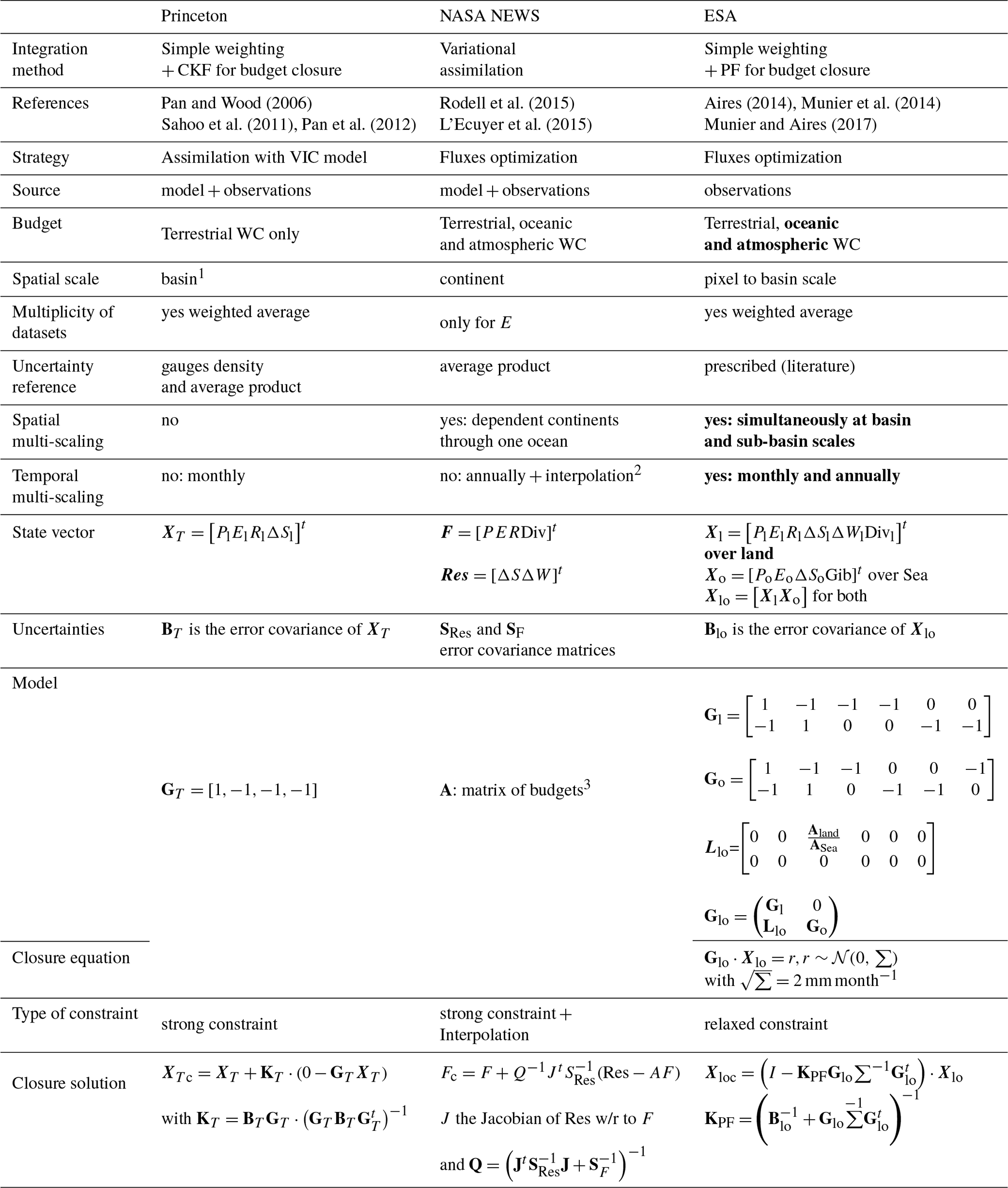
The ESA water cycle initiative – in the context of the ESA WATCHFUL project on water budget closure, Aires (2014) described several methodologies (Table 1) to integrate different hydrological datasets with a budget closure constraint. No surface or atmospheric models were used in these integration methods, making the obtained product interesting for model calibration and validation. One of the proposed methods, the so-called simple weighting + post-filtering (SW + PF), was applied by Munier et al. (2014) over the Mississippi basin, using satellite datasets for precipitation, evapotranspiration and water storage, and gauge observations for river discharge. After applying a budget closure constraint at the basin scale, the integrated components were compared to various in situ observations, showing good performances of the method. One of the main limitations is the dataset availability of the in situ river discharges. Another concern was the downscaling of the basin closure constraint to the pixel scale. A closure correction model (CCM) is a calibration of the EO that was developed based on the integrated product as the reference (Munier et al., 2014). It allows correction of each dataset independently to greatly reduce the budget residuals. This calibration was applied over the basins where river discharges are available and extended to the global scale using an index characterizing the various surface types (Munier and Aires, 2017). This type of post-processing step is anchored in the integration approach, but it can be applied to long time records, at any time or spatial resolution. It can even allow for the reconstruction of missing estimates.

In this paper, we propose several improvements of this line of research. In particular, we propose to close the WC budget not only over land, but also over ocean and in the atmosphere. Furthermore, the budget closure constraint is used simultaneously at different spatial (basin and sub-basin) and temporal (monthly and annual) scales. A new spatial interpolation scheme is proposed to downscale the basin-scale closure constraint to the pixel scale. This new framework is applied to the Mediterranean basin to provide an updated WC budget.

Section 2 presents the study domain and introduces the datasets used in the following. The integration approaches are described together with the other combination techniques in Sect. 3. Section 4 presents the evaluation metrics for the integrated product: its ability to close the WC and its validation with in situ data at the sub-basin or pixel scale. Section 5 presents the WC analysis for the period 2004–2009 using our resulting integrated dataset. Finally, Section 6 concludes the analysis and presents some perspectives. All notations used in the following are summarized in Table A1 in the Appendix.

2 Case study and datasets

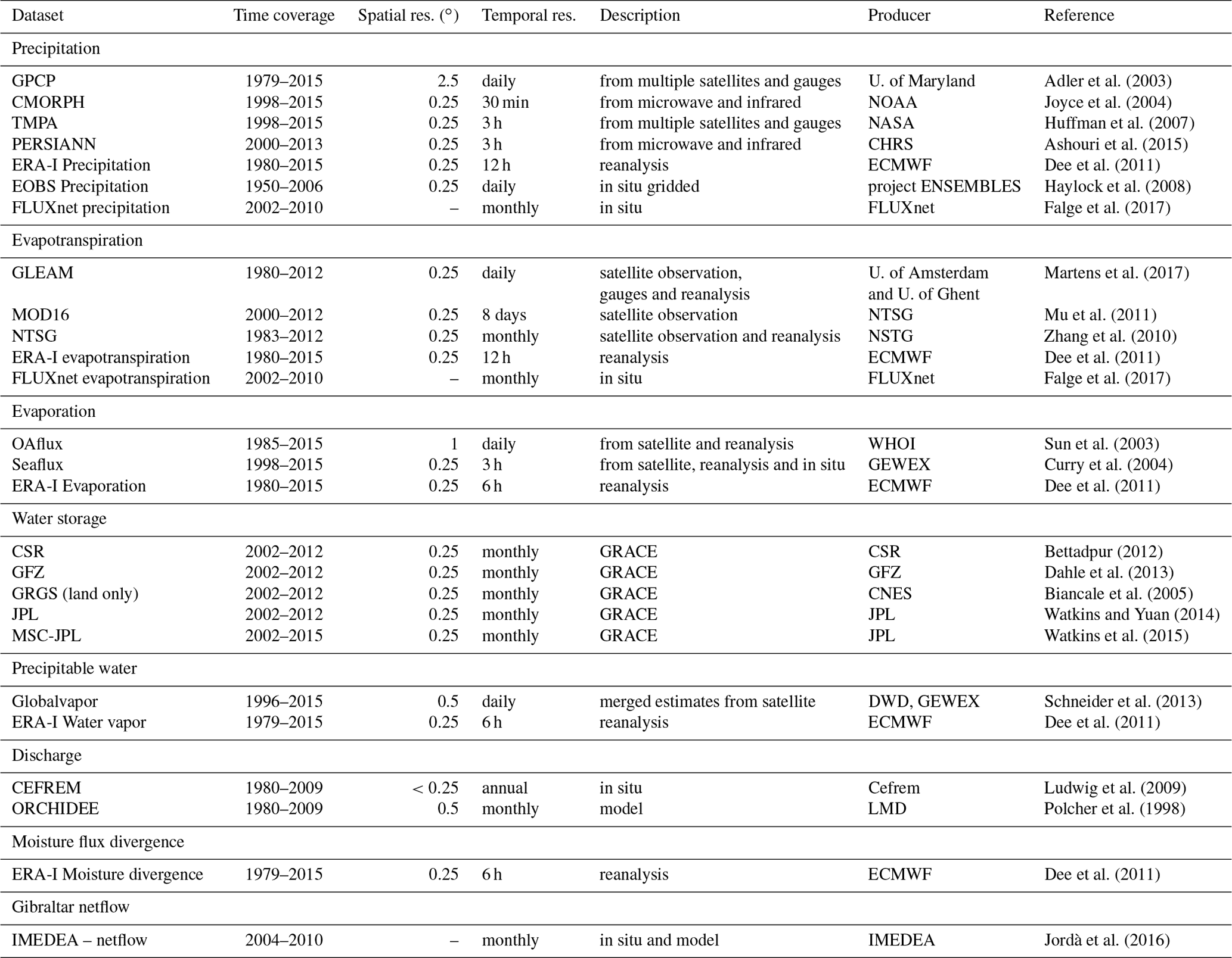
This section presents the spatial domain and the datasets used in this study. Table A2 in the Appendix summarizes the main characteristics of these products and more details can be found in Pellet et al. (2017). All products have different temporal extents but share a common coverage period 2004–2009.

2.1 Mediterranean region

The study domain is represented in Fig. 1. It is the catchment basin of the whole Mediterranean Sea drainage area, computed from each coastal pixel, including all rivers that flow into the sea. Basins have been computed using a hydrographic model (Wu et al., 2011) at a spatial resolution of 0.25^∘. The resolution of the hydrographic model used to compute the land–sea mask or catchment basin may have an impact on the spatial-average estimates and then on the WC budget residual. This area uncertainty is taken into account in the relaxation of the closure constraint at sub-basin scale (see Table 1). The Mediterranean Sea area (including the Black Sea) is 3.0 million km², and its drainage area is more than 5 million km².

Sub-basins were introduced in Pellet et al. (2017). They facilitate the analysis of local climate and specific hydrological features. The Mediterranean Sea and the terrestrial sub-basins used in the following are defined as

• the western Maghreb mainly based on the Atlas mountain discharge (MA-DZ-TN);

• the Nile basin and Libyan coast characterizing a Saharan and sub-Saharan climate (LY-EG);

• the Spanish coasts and Pyrénées (ES-Pyr);

• the French, Italian and Adriatic Sea coasts, carrying freshwater from the Alps and the Balkan mountains (Alp-IT-ADR);

• the eastern part of the Mediterranean Sea, Greece, Turkey and Israel (GR-TR-IL); and

• the whole Black Sea drainage catchment, Bulgaria, Georgia, Romania, Russia, Turkey, Ukraine, Slovakia, Hungary, Austria, Slovenia, Bosnia and Serbia (BLS).

In the current study, even if the closure method (PF) is applied over the LY-EG sub-basin, the high uncertainty of the Nile discharge and its particular climate (African monsoon) as well as anthropogenic conditions (most of its water is used for irrigation) make this sub-basin really different from the other sub-basins (Margat, 2004; Mariotti et al., 2002). Therefore the closure is ensured for the Nile sub-basin, but no spatial extension will be extrapolated over the LY-EG or the south (see Sect. 3).

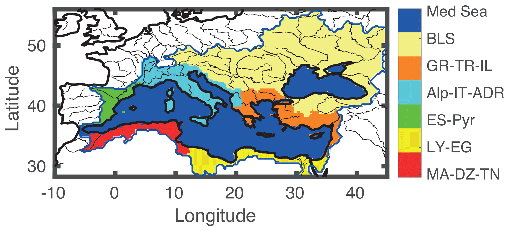
Figure 1 Region of interest. Sub-basins have been computed using a hydrological model (Wu et al., 2011), and rivers are from HydroShed (http://www.hydrosheds.org/, last access: 24 January 2019). See text for the definition of the sub-basins.

2.2 Original EO datasets

The datasets presented in this section will be used in the integration process. Most of them are satellite products and are commonly used for studying the WC. In order to integrate them, the datasets have been projected onto a common 0.25^∘ spatial resolution grid and re-sampled at the monthly scale.

Precipitation (P) – four satellite-based datasets have been selected. Two are gauge-calibrated products: the Tropical Rainfall Measuring Mission Multi-satellite Precipitation Analysis (TMPA, 3B42 V7) presented in Huffman et al. (2007) and the Global Precipitation Climatology Project (GPCP, v2) introduced by Adler et al. (2003). Two are uncalibrated products: Joyce et al. (2004) have unveiled the NOAA CPC Morphing Technique (CMORPH, v1) and Ashouri et al. (2015) developed the Precipitation Estimation from Remote Sensing Information using Artificial Neural Network (PERSIANN, v1). In this study, we use a mix of gauged/ungauged-calibrated precipitation datasets. This choice is motivated by the goal of preserving the original EO spatial pattern where limited gauge density in some areas may corrupt the signal during the gauge-calibration process (in TMPA and GPCP products).

Evapotranspiration (E) – three satellite-based products were chosen to describe evapotranspiration over land: the Global Land Evaporation Amsterdam Model (GLEAM-V3B, Martens et al., 2017; Miralles et al., 2011); the MODIS Global Evapotranspiration Project (MOD16, Mu et al., 2011); and the Numerical Terradynamic Simulation Group product (NSTG, Zhang et al., 2010).

Two products were chosen for the evaporation over the sea: the Objectively Analyzed air-sea Fluxes for Global Oceans (OAflux, Sun et al., 2003); and The Global Energy and Water Cycle Exchanges Project product (GEWEX-Seaflux, Curry et al., 2004).

Water storage change (ΔS) – the terrestrial and seawater storage datasets are all derived from the GRACE mission. The estimates of water storage implicitly include the underground water. Four satellite datasets are based on the spherical decomposition of GRACE measurement: the Jet Propulsion Laboratory (JPL, Watkins and Yuan, 2014) product; the Centre for Space Research (CSR, Bettadpur, 2012) product; the German Research Centre for Geoscience (GFZ, Dahle et al., 2013) product; and the land-only product from the Groupe de Recherche de Géodésie Spatiale (GRGS, Biancale et al., 2005). One extra solution based on the JPL-MASCONS decomposition of GRACE measurement (Watkins et al., 2015) is also used in this work. In order to compute the monthly change in water storage, we applied a centered derivative smoothing filter: [5∕24 3∕8 $-\mathrm{3}/\mathrm{8}$ $-\mathrm{5}/\mathrm{24}$] (Pellet et al., 2017). The filter is a slightly smoother version of the filter [1∕8 1∕4 $-\mathrm{1}/\mathrm{4}$ $-\mathrm{1}/\mathrm{8}$] presented by Eicker et al. (2016). It has been compared with several other filters (results not shown). The chosen filter is a good compromise between its smoothing (that suppresses information) and its ability to de-noise the time series.

Discharge (R_l) – no satellite-based product is available for the discharge with sufficient temporal extent and only a few rivers are still monitored by public or private networks for the Global Runoff Data Centre (GRDC) that collects discharge data at the global scale. The two discharge datasets used in the following are described in Pellet et al. (2017). Groundwater discharge is neglected and considered as an uncertainty source.

The CEFREM-V2 dataset of coastal annual discharge into the Mediterranean Sea (Ludwig et al., 2009) is based on in situ observations and some indirect estimates using the Pike formula (Pike, 1964). In addition, the Laboratoire de Météorologie Dynamique developed the Organising Carbon and Hydrology In Dynamic Ecosystems (ORCHIDEE, Polcher et al., 1998; Ducharne et al., 2003) land surface model chosen here to describe the monthly dynamics of the discharge. Two coastal discharges are available from its routing scheme with two different precipitation forcings: GPCC and Climatic Research Unit (CRU) products. We therefore projected the monthly dynamical patterns from ORCHIDEE towards the CEFREM grid. We then scaled the monthly values of ORCHIDEE to match the CEFREM annual values. For comparison purposes, CEFREM total freshwater inflow into the Mediterranean (without the Black Sea) is 400 km³ yr⁻¹, while ORCHIDEE gives a value of 380 km³ yr⁻¹. The scaling is then a simple way to take into account the anthropogenic impact that is not modeled at the annual scale and the 0.5^∘ resolution. The final product then has the spatial resolution and the annual cumulative value of CEFREM, but with the monthly dynamics of the ORCHIDEE model.

Precipitable water change (ΔW) – we considered two datasets for the precipitable water: the ESA Globvapor dataset (Schneider et al., 2013) and the 6 h reanalysis product from the ECMWF reanalyses (ERA-I, Dee et al., 2011). The ERA-I reanalysis has been considered here because precipitable water, although model-based, is largely constrained by satellite observations. In order to compute changes in precipitable water, we also applied the derivative filter: [5∕24 3∕8 $-\mathrm{3}/\mathrm{8}$ $-\mathrm{5}/\mathrm{24}$].

Moisture divergence (Div) – due to the limited temporal extent of the satellite-based data, we used the 6-hourly ERA-I reanalysis product (Dee et al., 2011). Among the various re-analyses, ERA-I was chosen here in view of previous results demonstrating advantages in the representation of long term wind variability (Stopa and Cheung, 2014) which plays a key role in the representation of moisture divergence. Nevertheless, Seager and Henderson (2013) have shown the limitation of the reanalysis that do not catch moisture divergence events shorter than at the 6 h. This limitation must be taken into account when closing the WC.

Gibraltar netflow (Gib) – the only multiannual estimate of the Gibraltar netflow based on observations is presented in Jordà et al. (2016). A monthly reconstruction of the net transport is used with the effects of the atmospheric pressure removed. This is done for consistency with the oceanic water storage from GRACE. The reconstruction technique used to generate that estimate has proven to be effective to simulate the variability but the uncertainties in the mean value stay large. In Jordà et al. (2017), an expert-based assessment of the mean transport is presented. Therefore, in this work we substituted the 2004–2016 mean value of the Jordà et al. (2016) estimate by the estimate proposed by Jordà et al. (2017).

The Mediterranean Sea is also connected to the Red Sea with the Suez channel and to the Black Sea with the Bosporus Strait. The netflow at the Suez channel is neglected (Mariotti et al., 2002; Harzallah et al., 2018). Since no in situ reference is available on the Bosporus netflow, the current work gathers the Mediterranean and the Black Sea into a single reservoir for the integration process. An a posteriori estimate of the Bosporus netflow will be given in Sect. 5 using the water budget equations and the integrated estimates for the other water components.

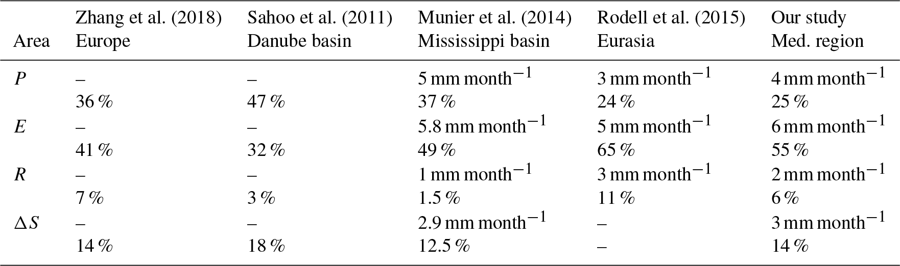
Zhang et al. (2018)Sahoo et al. (2011)Munier et al. (2014)Rodell et al. (2015)

Table 2 Comparison of the uncertainty specifications for terrestrial water components. The weights associated with a variable (computed as the ratio between the particular variable uncertainty with respect to the sum of all the uncertainties ${\mathit{\sigma }}_i^{\mathrm{2}}/\sum _i{\mathit{\sigma }}^{\mathrm{2}}$) are expressed in percentage.

2.3 Validation datasets

The ENSEMBLES observation dataset (EOBS) – in order to validate the precipitation, an additional dataset is used: the EOBS dataset developed by EU-FP6 project ENSEMBLES (Haylock et al., 2008). It was a regional, well-documented and validated in situ gridded daily dataset at the 0.25^∘ spatial resolution, covering the 1950–2007 period.

FLUXNET – ground-based FLUXNET data (Falge et al., 2017) were used to validate the evapotranspiration and precipitation over several sites in Europe¹. These flux measurements were based on a eddy covariance technique. All stations available in Europe for the 2004–2009 period have been selected. In order to avoid coastal contamination, the three seaside towers IT-Ro2, IT-Noe and ES-Amo have been suppressed.

Total and thermosteric sea-level databases – to validate the sea-level output from the integration technique, we use an independent estimate of the Mediterranean water content. The water content can be estimated as total sea level minus the thermosteric variations (i.e., changes in sea level due to thermal expansion/contraction) (Fenoglio-Marc et al., 2006; Jordà and Gomis, 2006). Total sea level is obtained from the Ssalto/Duacs altimeter data that are produced and distributed by the Copernicus Marine and Environment Monitoring Service². The thermosteric sea-level variations are estimated using two ocean regional reanalyses (MEDRYS, Hamon et al., 2016; Bahurel et al., 2012, MyOcean,) and two global products that include the Mediterranean Sea (the Met Office Hadley Centre EN-v4 Good et al., 2013; Ishii et al., 2003, ISHII).

2.4 EO uncertainty assumptions

Some studies aimed to characterize the uncertainty of satellite-retrieved products: estimating the relative uncertainty of numerous datasets by the distance to the average product (Pan et al., 2012; Zhang et al., 2016) or using non-satellite datasets (Sahoo et al., 2011). Nevertheless, such characterizations are generally product- and site-specific, and for some products used in this work, no uncertainty characterization can be found in the literature. For these reasons we considered the same uncertainty as in Aires (2014).

Table 2 summarizes the uncertainty used in the various integration techniques. The uncertainty is associated with a weight which is the ratio of the sum of all the uncertainties in the WC equation and the uncertainty of the considered variable (computed as ${\mathit{\sigma }}_i^{\mathrm{2}}/\sum _i{\mathit{\sigma }}^{\mathrm{2}}$ and expressed in percentage). Note that uncertainties in Table 2 stand for the merged product and not for a particular satellite dataset (see Eq. 6). The uncertainties are prescribed by the literature, but they are slightly modified from Munier et al. (2014) to handle the special case of the Mediterranean region. Munier et al. (2014) used uncertainty values of 10 mm month⁻¹ for each of the four P products and the three E products (leading to 5 and 5.8 mm month⁻¹ for the merged P and E estimate), 5 mm month⁻¹ for each of the three ΔS products (leading to 2.9 mm month⁻¹ for the merged product) and 1 mm month⁻¹ for only one R. The choice of these values was motivated by results of the studies cited in Sect. 1. In order to be closer to Rodell et al. (2015), on the one hand, we decide to reduce P uncertainty to 4 mm month⁻¹. This is justified since the de-biasing was done toward the gauge-calibrated TMPA dataset (see Pellet et al., 2017, for details). On the other hand, we increased E uncertainty up to 6 mm month⁻¹. The uncertainty of the merged ΔS is estimated to be broadly the same since it is mainly driven by the large pixel resolution of GRACE. Finally, the uncertainty of the discharge R has been increased since the product is partially based on model simulations and the groundwater discharge is not included in the analysis (see Sect. 2). For the atmospheric variables, we consider an uncertainty proportional to the range of variability for the precipitable water change: 1 mm month⁻¹. Following the suggestion from Seager and Henderson (2013), the reanalysis moisture divergence uncertainty has been set to 6 mm month⁻¹ due to its large range of variability and timescale.

3 EO integration methodologies

3.1 Closing the water cycle budget

In this section, the notations are introduced, but additional details can be found in Aires (2014). The WC can be described by the following time-varying budget equations:

$$\begin{array}{ll}{\displaystyle }& {\displaystyle \frac{\mathit{\delta }{S}_{\mathrm{l}}}{\mathit{\delta }t}}=P_{\mathrm{l}}-E_{\mathrm{l}}-R_{\mathrm{l}}\left(\mathrm{terrestrial}\right),\\ {\displaystyle }& {\displaystyle \frac{\mathit{\delta }{S}_{\mathrm{o}}}{\mathit{\delta }t}}=P_{\mathrm{o}}-E_{\mathrm{o}}+R_{\mathrm{l}}^{*}-\mathrm{Gib}\left(\mathrm{oceanic}\right),\\ \text{(1)}& {\displaystyle }& {\displaystyle \frac{\mathit{\delta }W}{\mathit{\delta }t}}=E_{\mathrm{l}/\mathrm{o}}-P_{\mathrm{l}/\mathrm{o}}-\mathrm{Div}\left(\mathrm{atmospheric}\right),\end{array}$$

where “l” stands for land and “o” for ocean. If all the components in Eq. (1) are expressed in mm month⁻¹ (area-normalized), then a fourth equality is defined: $R_{\mathrm{l}}^{*}=\frac{{\mathbf{A}}_{\mathrm{land}}}{{\mathbf{A}}_{\mathrm{Sea}}}\cdot R_{\mathrm{l}}$ for total freshwater input/output with A_land is the total drainage area of the Mediterranean (including the Black Sea), and A_Sea is the total area of both seas.

We first consider the six terrestrial water components ${\mathit{X}}_{\mathrm{l}}^{\mathrm{t}}=(P_{\mathrm{l}}$, E_l, R_l, ΔS_l, ΔW_l, Div_l) and the six oceanic water components ${\mathit{X}}_{\mathrm{o}}^{\mathrm{t}}=(P_{\mathrm{o}}$, E_o, ΔS_o, ΔW_o, Div_o, Gib). We then define ${\mathit{X}}_{\mathrm{lo}}^{\mathrm{t}}=[{\mathit{X}}_{\mathrm{l}}$, X_o]^t. The closure of the water budget can be relaxed using a centered Gaussian random variable r and ${\mathit{X}}^{\mathrm{t}}\cdot {\mathbf{G}}_{\mathrm{lo}}^{\mathrm{t}}=\mathit{r}$, with r∼𝒩(O, ∑) where

$$\begin{array}{ll}{\displaystyle }& {\displaystyle }{\mathbf{G}}_{\mathrm{lo}}=\\ \text{(2)}& {\displaystyle }& {\displaystyle }\left[\begin{array}{cccccccccccc}\mathrm{1}& -\mathrm{1}& -\mathrm{1}& -\mathrm{1}& \mathrm{0}& \mathrm{0}& \mathrm{0}& \mathrm{0}& \mathrm{0}& \mathrm{0}& \mathrm{0}& \mathrm{0}\\ -\mathrm{1}& \mathrm{1}& \mathrm{0}& \mathrm{0}& -\mathrm{1}& -\mathrm{1}& \mathrm{0}& \mathrm{0}& \mathrm{0}& \mathrm{0}& \mathrm{0}& \mathrm{0}\\ \mathrm{0}& \mathrm{0}& {\displaystyle \frac{{\mathbf{A}}_{\mathrm{land}}}{{\mathbf{A}}_{\mathrm{Sea}}}}& \mathrm{0}& \mathrm{0}& \mathrm{0}& \mathrm{1}& -\mathrm{1}& -\mathrm{1}& \mathrm{0}& \mathrm{0}& -\mathrm{1}\\ \mathrm{0}& \mathrm{0}& \mathrm{0}& \mathrm{0}& \mathrm{0}& \mathrm{0}& -\mathrm{1}& \mathrm{1}& \mathrm{0}& -\mathrm{1}& -\mathrm{1}& \mathrm{0}\end{array}\right]\end{array}$$

which is equivalent to the water budget in Eq. (1) and

$${\displaystyle }{\displaystyle }\mathrm{\Sigma }=\left(\begin{array}{cc}{\mathit{\sigma }}_{\mathrm{l}}^{\mathrm{2}}& \mathrm{0}\\ \mathrm{0}& {\mathit{\sigma }}_{\mathrm{o}}^{\mathrm{2}}\end{array}\right),$$

with ${\mathit{\sigma }}_{\mathrm{l}}=\left(\begin{array}{cc}\mathrm{2}& \mathrm{0}\\ \mathrm{0}& \mathrm{2}\end{array}\right)$ representing the standard deviation of the constrained terrestrial and atmospheric water budget residual over land, and ${\mathit{\sigma }}_{\mathrm{o}}=\left(\begin{array}{cc}\mathrm{2}& \mathrm{0}\\ \mathrm{0}& \mathrm{2}\end{array}\right)$ representing the standard deviations of the constrained oceanic and atmospheric water budget residual over sea. Σ assumes no correlation in the imbalance of the three WCs at monthly and annual scales, at sub-basin scales or entire basin scales.

Let

$$\begin{array}{}\text{(3)}& {\displaystyle }{\displaystyle }{\mathit{Y}}_{\mathrm{l}}^{\mathrm{t}}=\left(\begin{array}{lll}(P_{\mathrm{1}},\mathrm{\dots },P_{\mathrm{p}},& E_{\mathrm{1}},\mathrm{\dots },E_q,& R_{\mathrm{1}},\mathrm{\dots },R_r,\\ \mathrm{\Delta }{S}_{\mathrm{1}},\mathrm{\dots },\mathrm{\Delta }{S}_{\mathrm{s}},& \mathrm{\Delta }{W}_{\mathrm{1}},\mathrm{\dots },\mathrm{\Delta }{W}_v,& {\mathrm{Div}}_{\mathrm{1}},\mathrm{\dots },{\mathrm{Div}}_{\mathrm{d}})\end{array}\right)\end{array}$$

be the vector of dimension $n_{\mathrm{l}}=p+q+m+s+v+d$ gathering the multiple observations available for each water component over land (similarly Y_o of dimension n_o is defined over sea):

• (P₁, P₂, …, P_p), the “p” precipitation estimates;

• (E₁, E₂, …, E_q), the q sources of information for evapotranspiration;

• (R₁, R₂, …, R_m), the m discharge estimates;

• (ΔS₁, ΔS₂, …, ΔS_s), the “s” sources of information for the water storage change;

• (ΔW₁, ΔW₂, …, ΔW_v), the v precipitable water change estimates;

• (Div₁, Div₂, …, Div_d), the “d” moisture divergence.

The aim of this approach is to obtain a linear filter K_an used to obtain an estimate X_an (“an” stands for analysis) of X_lo based on the observations Y_lo:

$$\begin{array}{}\text{(4)}& {\displaystyle }{\displaystyle }{\mathit{X}}_{\mathrm{an}}={\mathbf{K}}_{\mathrm{an}}\cdot {\mathit{Y}}_{\mathrm{lo}}\mathrm{with}{\mathit{Y}}_{\mathrm{lo}}=\left[{\mathit{Y}}_{\mathrm{l}},{\mathit{Y}}_{\mathrm{o}}\right],\end{array}$$

where K_an is a $\mathrm{12}\times (n_{\mathrm{l}}+n_{\mathrm{o}})$ matrix.

3.2 Simple weighting (SW)

A general approach to deal with EO datasets in the analysis of the WC is to choose the best individual dataset for each water component. This is the approach developed, for example, in the GEWEX project. In Pellet et al. (2017), an optimal selection (OS) was based on the minimization of the water budget residuals to select the best combination of individual datasets. Using the OS principle facilitates finding datasets coherent to each other and with independent errors (Rodell et al., 2015). But this kind of strategy limits the use of several sources of information to reduce the uncertainties.

On the other hand, the SW approach benefits from the multiplicity of the observations. EO products, and more generally any estimation of a variable via observations, present two types of errors. (1) Systematic errors related, for instance, to the absolute calibration of the sensor. These can be represented by a bias and/or a scaling factor. (2) Random errors related to retrieval algorithm uncertainties or to missing or inaccurate auxiliary information (e.g., cloud mask) or to the sensor itself. These are often characterized by a standard deviation using a Gaussian hypothesis. From a statistical point of view, using the average of several estimates reduces the random errors of the estimation if no bias errors are present in the estimates. The merging process such as in Eq. (4) requires unbiased estimates (Aires, 2014). The difficulty is that, as for uncertainties (Sect. 2.4), it is rather difficult to obtain bias estimates from the literature for every dataset used in this approach. A pragmatic strategy is to set the reference as the mean state for each component. Then, all the sources of information for this component are bias-corrected toward this reference (Munier and Aires, 2017). A slightly modified version of the bias correction is to choose one reference among the datasets and apply the bias correction. We opted for the modified version and de-biased the EO using the climatological season of the TMPA product as a reference (Pellet et al., 2017). Therefore, our SW methodology is first based on a seasonal bias correction to reduce the systematic biases and is then followed by a weighted average of the corrected estimates to reduce the random errors. After the seasonal de-biasing, all the precipitation products will have a similar seasonality, but their inter-annual trend or monthly variations will still be different. In particular, the seasonal de-biasing will not change the trend of the EO products.

The SW methodology uses the diversity of datasets to reduce the random errors. Let us consider the p precipitation observations P_i associated with Gaussian errors ϵ_i∼𝒩(O, σ_i). σ_i is the standard deviation of the ith estimate. The SW precipitation estimate P_SW is given by the weighted average:

$$\begin{array}{}\text{(5)}& {\displaystyle }{\displaystyle }{P}_{\mathrm{SW}}={\displaystyle \frac{\mathrm{1}}{p-\mathrm{1}}}\sum _{i=\mathrm{1}}^p{\displaystyle \frac{\sum _{k\ne i}{\left({\mathit{\sigma }}_k\right)}^{\mathrm{2}}}{\sum _k{\left({\mathit{\sigma }}_k\right)}^{\mathrm{2}}}}{P}_i.\end{array}$$

This equation is valid when there is no bias error in the P_is (thanks to the preliminary bias correction) and is optimal when the errors ϵ_i are statistically independent of each other. This expression is valid for the other water components. The variance of the P_SW uncertainties is then given by

$$\begin{array}{}\text{(6)}& {\displaystyle }{\displaystyle }{\mathit{\sigma }}_{P_{\mathrm{SW}}}={\displaystyle \frac{\mathrm{1}}{(p-\mathrm{1}{)}^{\mathrm{2}}}}\sum _{i=\mathrm{1}}^p{\left({\displaystyle \frac{\sum _{k\ne i}{\left({\mathit{\sigma }}_k\right)}^{\mathrm{2}}}{\sum _k{\left({\mathit{\sigma }}_k\right)}^{\mathrm{2}}}}\right)}^{\mathrm{2}}{\mathit{\sigma }}_i^{\mathrm{2}}.\end{array}$$

This is important information because it gives the uncertainty of the estimates in Eq. (5). It shows that the P_SW errors can be significantly reduced by increasing the number p of observations.

Following Eq. (5) the SW state vector X_SW can be defined as

$$\begin{array}{}\text{(7)}& {\displaystyle }{\displaystyle }{\mathit{X}}_{\mathrm{SW}}={\mathbf{K}}_{\mathrm{SW}}\cdot {\mathit{Y}}_{\mathrm{lo}},\end{array}$$

where K_SW is a $\mathrm{12}\times (n_{\mathrm{l}}+n_{\mathrm{o}})$ matrix in which each line represents Eq. (5) for 1 of the 12 water components (the first one for the precipitation estimate, the second for the evapotranspiration, etc.) and based on the (n_l+n_o) observations. Since no specific uncertainty specifications were available in the literature for the Mediterranean basin, the uncertainties are assumed to have the same standard deviation σ_i in the following.

3.3 Post-filtering (PF)

In the SW approach, each water component is weighted (see Eqs. 6–7) based on its a priori uncertainty (Sect. 2), but no closure constraint is imposed on the solution X_SW. Several methods were considered in Aires (2014) to introduce a WC budget closure constraint on the SW solution. However, Monte Carlo simulations have shown that the SW solution associated with a so-called post-filtering (PF) provides results as good as more complex techniques such as variational assimilation.

The PF approach has been introduced (Pan and Wood, 2006) to impose the closure constraint on a previously obtained solution. Here we use X_SW as the first guess on the state vector X_lo. In Aires (2014), the PF was used and tested without any model, as a simple post-processing step after the SW. Following Yilmaz et al. (2011), the current study implements the PF filter with a relaxed closure constraint characterized by its uncertainty covariance ∑:

$$\begin{array}{}\text{(8)}& {\displaystyle }{\displaystyle }{\mathit{X}}_{\mathrm{PF}}=\left(I-{\mathbf{K}}_{\mathrm{PF}}\cdot {\mathbf{G}}_{\mathrm{lo}}{\mathrm{\Sigma }}^{-\mathrm{1}}{\mathbf{G}}_{\mathrm{lo}}^{\mathrm{t}}\right)\cdot {\mathit{X}}_{\mathrm{SW}},\end{array}$$

where $K_{\mathrm{PF}}=({\mathbf{B}}_{\mathrm{lo}}^{-\mathrm{1}}+{\mathbf{G}}_{\mathrm{lo}}\sum ^{-\mathrm{1}}{\mathbf{G}}_{\mathrm{lo}}^{\mathrm{t}}{)}^{-\mathrm{1}}$ and B_lo is the error covariance matrix of the first estimate on X_lo.

We can make X_SW explicit to obtain the linear operator K_an of Eq. (4):

$$\begin{array}{}\text{(9)}& {\displaystyle }{\displaystyle }{\mathit{X}}_{\mathrm{an}}={\mathit{X}}_{\mathrm{PF}}=\left(I-{\mathbf{K}}_{\mathrm{PF}}\cdot {\mathbf{G}}_{\mathrm{lo}}{\mathrm{\Sigma }}^{-\mathrm{1}}{\mathbf{G}}_{\mathrm{lo}}^{\mathrm{t}}\right)\cdot K_{\mathrm{SW}}\cdot {\mathit{Y}}_{\mathrm{lo}},\end{array}$$

so that $K_{\mathrm{an}}=(\mathbf{I}-{\mathbf{K}}_{\mathrm{PF}}\cdot {\mathbf{G}}_{\mathrm{lo}}{\mathrm{\Sigma }}^{-\mathrm{1}}{\mathbf{G}}_{\mathrm{lo}}^{\mathrm{t}})\cdot K_{\mathrm{SW}}$. The PF step (budget closure) consists in partitioning the budget residual among the 12 components at each time step, independently. This technique allows a satisfactory WC budget closure for each basin to be obtained. The residual term r could be reduced in the SW + PF approach by decreasing the variance Σ in Eq. (8). Nevertheless, an excessively tight closure constraint is in contradiction with the large inherent uncertainties in original observations.

Following Munier et al. (2014) we enforced the budget closure by frequency range to avoid high-frequency errors impacting the low-frequency variables such as the evapotranspiration (mainly driven by annual vegetation growth; Allen et al., 1998). We first decomposed each parameter into high- and low-frequency components considering a cut-off frequency of 6 months (using a FFT decomposition). The budget is then applied independently at low and high frequencies. The high-frequency component of E is then not included in the high budget closure. The linearity of PF and FFT ensures the budget closure of the re-composed final product. In the following temporal multi-scaling, the annual constraint is applied only to the low-frequency budget closure.

Spatial multi-scaling – it is possible to impose a WC budget closure simultaneously over the six sub-basins, the full basin and the ocean (i.e., Mediterranean and Black Sea). Let us consider the total WC state vector

$$\begin{array}{}\text{(10)}& {\displaystyle }{\displaystyle }{\mathit{X}}^{\mathrm{t}}={\left[{\mathit{X}}_{\mathrm{l}}^{\left(\mathrm{1}\right)},{\mathit{X}}_{\mathrm{l}}^{\left(\mathrm{2}\right)},{\mathit{X}}_{\mathrm{l}}^{\left(\mathrm{3}\right)},{\mathit{X}}_{\mathrm{l}}^{\left(\mathrm{4}\right)},{\mathit{X}}_{\mathrm{l}}^{\left(\mathrm{5}\right)},{\mathit{X}}_{\mathrm{l}}^{\left(\mathrm{6}\right)},{\mathit{X}}_{\mathrm{o}}\right]}^{\mathrm{t}}\end{array}$$

that includes the six water components ${\mathit{X}}_{\mathrm{l}}^i$ over each sub-basin i of area ${\mathbf{A}}_{\mathrm{l}}^{\left(i\right)}$ and ocean. The “closure” matrix becomes

$$\begin{array}{}\text{(11)}& {\displaystyle }{\displaystyle }{\mathbf{G}}_{\mathrm{lo}}=\left(\begin{array}{ccccc}{\mathbf{G}}_{\mathrm{l}}^{\left(\mathrm{1}\right)}& \mathrm{0}& \mathrm{\cdots }& \mathrm{0}& \mathrm{0}\\ \mathrm{0}& {\mathbf{G}}_{\mathrm{l}}^{\left(\mathrm{2}\right)}& \mathrm{\cdots }& \mathrm{0}& \mathrm{0}\\ \mathrm{\cdots }& \mathrm{\cdots }& \mathrm{\cdots }& \mathrm{\cdots }& \mathrm{\cdots }\\ \mathrm{0}& \mathrm{0}& \mathrm{\cdots }& {\mathbf{G}}_{\mathrm{l}}^{\left(\mathrm{6}\right)}& \mathrm{0}\\ {\mathbf{L}}_{\mathrm{lo}}^{\left(\mathrm{1}\right)}& {\mathbf{L}}_{\mathrm{lo}}^{\left(\mathrm{2}\right)}& \mathrm{\cdots }& {\mathbf{L}}_{\mathrm{lo}}^{\left(\mathrm{6}\right)}& {\mathbf{G}}_{\mathrm{o}}\end{array}\right)\end{array}$$

with

$$\begin{array}{ll}{\displaystyle }& {\displaystyle }{\mathbf{G}}_{\mathrm{l}}^{\left(i\right)}=\left[\begin{array}{cccccc}\mathrm{1}& -\mathrm{1}& -\mathrm{1}& -\mathrm{1}& \mathrm{0}& \mathrm{0}\\ -\mathrm{1}& \mathrm{1}& \mathrm{0}& \mathrm{0}& -\mathrm{1}& -\mathrm{1}\end{array}\right],\\ {\displaystyle }& {\displaystyle }{\mathbf{L}}_{\mathrm{lo}}^{\left(i\right)}=\left[\begin{array}{cccccc}\mathrm{0}& \mathrm{0}& {\displaystyle \frac{{\mathbf{A}}_{\mathrm{l}}^{\left(i\right)}}{{\mathbf{A}}_{\mathrm{Sea}}}}& \mathrm{0}& \mathrm{0}& \mathrm{0}\\ \mathrm{0}& \mathrm{0}& \mathrm{0}& \mathrm{0}& \mathrm{0}& \mathrm{0}\end{array}\right],\\ \text{(12)}& {\displaystyle }& {\displaystyle }{\mathbf{G}}_{\mathrm{o}}=\left[\begin{array}{cccccc}\mathrm{1}& -\mathrm{1}& -\mathrm{1}& \mathrm{0}& \mathrm{0}& \mathrm{1}\\ -\mathrm{1}& \mathrm{1}& \mathrm{0}& -\mathrm{1}& -\mathrm{1}& \mathrm{0}\end{array}\right].\end{array}$$

The last row of G_lo represents the overall budget closure, including all the sub-basins and the ocean. The dimensions of the covariance matrices B_lo and ∑ are increased following the new size of the state vector X_lo. No cross terms in B_lo and ∑ are included, meaning that there is no dependency of the first guess and closure errors among the sub-basins.

Temporal multi-scaling – it is also possible to impose a WC budget closure simultaneously at monthly and annual scales. With monthly closure, the annual closure should automatically be obtained, but due to the relaxation of the closure constraint, the annual closure would be relaxed too. We control here the yearly closure constraint with an uncertainty of 1 mm. Furthermore, we impose a yearly closure assuming no groundwater storage change at the annual scale over land (representing an additional constraint on ΔS_l to ensure that no bias is introduced for this variable during the PF process). In this framework, monthly closures are now interdependent in the given year and the new state vector is

$$\begin{array}{}\text{(13)}& {\displaystyle }{\displaystyle }{\mathit{X}}_{\mathrm{year}}^{\mathrm{t}}={\left[{\mathit{X}}^{\mathrm{Jan}},\mathrm{\cdots },{\mathit{X}}^{\mathrm{Dec}}\right]}^{\mathrm{t}},\end{array}$$

with X^m the total state vector X defined in Eq. (10), for month m. The closure is applied independently for the 4 years of the 2004–2009 period, but the 12 months of each year are closed independently.

The closure matrix GA_lo that includes closure for the 12 months of the year and the full year is derived from the monthly constraint of Eq. (11) and defined as

$$\begin{array}{}\text{(14)}& {\displaystyle }{\displaystyle }{\mathbf{GA}}_{\mathrm{lo}}=\left(\begin{array}{cccc}{\mathbf{G}}_{\mathrm{lo}}& \mathrm{0}& \mathrm{\cdots }& \mathrm{0}\\ \mathrm{0}& {\mathbf{G}}_{\mathrm{lo}}& \mathrm{\cdots }& \mathrm{0}\\ \mathrm{\cdots }& \mathrm{\cdots }& \mathrm{\cdots }& \mathrm{\cdots }\\ \mathrm{0}& \mathrm{0}& \mathrm{\cdots }& {\mathbf{G}}_{\mathrm{lo}}\\ {\mathbf{N}}_{\mathrm{lo}}& {\mathbf{N}}_{\mathrm{lo}}& \mathrm{\cdots }& {\mathbf{N}}_{\mathrm{lo}}\end{array}\right),\end{array}$$

where N_lo is the modified closure matrix G_lo in which the matrix ${\mathbf{G}}_{\mathrm{l}}^{\left(i\right)}$ is rewritten in ${\mathbf{N}}_{\mathrm{l}}^{\left(i\right)}$ by imposing ΔS_l=0:

$$\begin{array}{}\text{(15)}& {\displaystyle }{\displaystyle }{\mathbf{N}}_{\mathrm{l}}^{\left(i\right)}=\left[\begin{array}{cccccc}\mathrm{1}& -\mathrm{1}& -\mathrm{1}& \mathbf{0}& \mathrm{0}& \mathrm{0}\\ -\mathrm{1}& \mathrm{1}& \mathrm{0}& \mathrm{0}& -\mathrm{1}& -\mathrm{1}\end{array}\right].\end{array}$$

The last row of GA_lo represents the annual budget closure considering no storage change at the annual scale over land, including all the sub-basins and the ocean. The dimensions of the covariance matrices B_lo and ∑ are increased once again following the new size of the state vector X_year. No cross terms in B_lo and ∑ are included, meaning that there is no dependency of the first guess and closure errors between the months.

This SW + PF technique is able to deal only with time series (average value over the considered sub-basins), not with maps (pixel), since the discharge is not available at this resolution. Therefore, in order to obtain a multi-component dataset that closes the WC budget and has spatial patterns at the pixel level, another technique needs to be used.

3.4 INTegration (INT)

The INT methodology allows one to extrapolate the results obtained with the previous SW + PF, from the sub-basin to pixel scales. To obtain a pixel-wise closure, Zhang et al. (2018) assimilate satellite data into the VIC model at the pixel scale (0.5^∘) using the VIC pixel water storage and runoff information. Munier and Aires (2017) extrapolated at the global scale the results of the WC closure of several large river basins around the globe, by using surface classes that intend to discriminate between EO error types, preserving as much as possible the hydrological coherency.

The INT approach proposed here uses the WC closure over the Mediterranean sub-basins to extrapolate the closure correction to the surrounding area. The methodology is presented in its various steps in Fig. 2 for precipitation and evaporation, for a particular month. In this analysis, we consider only the Mediterranean sub-basins and their close neighborhood, so a simple spatial interpolation of the closure correction is assumed to be sufficient.

The SW + PF method (Fig. 2, second row) provides a WC budget closure over the six sub-basins, for each month $m=\mathrm{1},\mathrm{\cdots },\mathrm{72}$ of the 2004–2009 period.

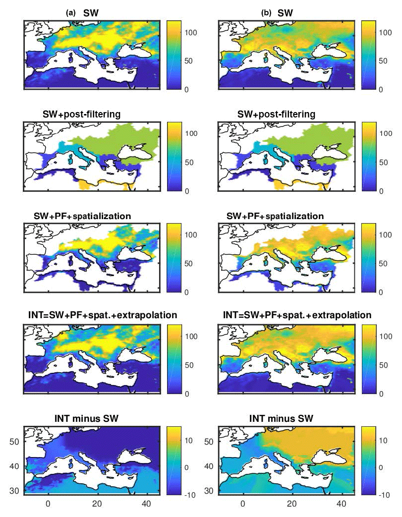
Figure 2 Steps of the spatialization of the budget closure for the INT solution, from the SW to the INT solutions: precipitation (a) and evapotranspiration (b) for July 2008. Units are in mm month⁻¹.

The INT method requires a scaling factor to go from the SW to the SW + PF solution at the sub-basin scale. We define ${\mathit{\beta }}^{\left(i\right)}\left(m\right)=P_{\mathrm{PF}}^{\left(i\right)}\left(m\right)/P_{\mathrm{SW}}^{\left(i\right)}\left(m\right)$ (for precipitation here), the ratio between the SW and the SW + PF solution, for each sub-basin i and month m. This ratio can be used to scale the SW dataset towards the SW + PF solution at the basin scale, for a particular month m, in the following way:

$$\begin{array}{}\text{(16)}& {\displaystyle }{\displaystyle }{P}_{\mathrm{INT}}^{\left(i\right)}\left(m\right)={\mathit{\beta }}^{\left(i\right)}\left(m\right)\cdot P_{\mathrm{SW}}^{\left(i\right)}\left(m\right)\left(=P_{\mathrm{PF}}^{\left(i\right)}\left(m\right)\right).\end{array}$$

For water storage change or moisture divergence, this β could become negative. In this case, the bias correction ${\mathit{\gamma }}^{\left(i\right)}\left(m\right)=P_{\mathrm{PF}}^{\left(i\right)}\left(m\right)-P_{\mathrm{SW}}^{\left(i\right)}\left(m\right)$ is used instead:

$$\begin{array}{}\text{(17)}& {\displaystyle }{\displaystyle }\mathrm{\Delta }{S}_{\mathrm{INT}}^{\left(i\right)}\left(m\right)=\mathrm{\Delta }{S}_{\mathrm{SW}}^{\left(i\right)}\left(m\right)+{\mathit{\gamma }}^{\left(i\right)}\left(m\right)\left(=\mathrm{\Delta }{S}_{\mathrm{PF}}^{\left(i\right)}\left(m\right)\right).\end{array}$$

The β scaling is defined at the sub-basin scale, but if interpolated spatially, it could be used at the pixel scale to obtain a truly spatialized solution.

Let us define a scaling map at the pixel level α such that for each pixel j in sub-basin i, for each month m, α(j, m)=β⁽ⁱ⁾(m) (or γ⁽ⁱ⁾(m)). When used as it is, the convolution of SW and α maps allows for the spatialization of the sub-basins' closure (Fig. 2, third row) with

$$\begin{array}{}\text{(18)}& {\displaystyle }{\displaystyle }\underset{j\in {\mathbf{A}}_{\mathrm{l}}^{\left(i\right)}}{\iint }{P}_{\mathrm{SW}}(j,m)\dot{\mathit{\alpha }}(j,m)={\mathit{\beta }}^{\left(i\right)}\left(m\right)\cdot P_{\mathrm{SW}}^{\left(i\right)}\left(m\right)=P_{\mathrm{INT}}^{\left(i\right)}\left(m\right).\end{array}$$

However, this product presents not only a discontinuity across the sub-basins (where different scaling factors β are defined) but also no value can be provided outside of the sub-basins.

To solve these two issues, the α scaling maps are interpolated/extrapolated.

• Interpolation – a region of 200 km on either side of the frontier between two sub-basins i₁ and i₂ is defined, and a smooth interpolation is performed between the two scaling factors ${\mathit{\beta }}^{\left(i_{\mathrm{1}}\right)}\left(m\right)$ and ${\mathit{\beta }}^{\left(i_{\mathrm{2}}\right)}\left(m\right)$ based on the distance to the frontier. This interpolation of the scaling factors α between two sub-basins can introduce errors (closure residuals can slightly increase), but it will be shown that this effect is limited and that the bottom equations (in parenthesis) in Eqs. (16)–(17) stand overall.

• Extrapolation – an extrapolation of the α maps is then performed to have a scaling factor α outside of the sub-basin domain. This extrapolation is weighted according to the respective distances to the two closest sub-basins.

The INT product is the convolution between the SW dataset with the resulting scaling map α that constrains the WC budget closure. INT is then an optimized version of SW in which the WC budget closure correction has been extended at the pixel scale. The fourth row of Fig. 2 shows the resulting INT product and its spatial coverage. The continuity issues between the sub-basins have been solved, and the extrapolation allows for a spatial coverage over the entire domain.

The extrapolation of a closure constraint is interesting at the technical level because for other regions, or when working at the global scale, some form of interpolation/extrapolation between the monitored sub-basins is required (Munier and Aires, 2017). The extrapolation outside of the Mediterranean region will also allow for the use of more in situ observations for the evaluation; this will help the testing of the generalization ability of the extrapolation scheme. The justification of this interpolation/extrapolation is based on the assumption that most of the WC imbalance is due to satellite errors (this assumption is used for the CAL methodology too). The closure constraint is supposed to improve the satellite estimate by reducing the bias and random errors. If no other information is used (such as surface type; see Munier and Aires, 2017), the EO errors can be considered spatially continuous, and it then makes sense to extrapolate results based on this spatial continuity. We perform the main analysis over the Mediterranean basin and test the extrapolation scheme over well-monitored locations.

The difference between the SW and INT estimates, represented in the last row of Fig. 2, is then directly related to the pixel-wise interpolated scaling factor α. Discontinuity between the sub-basins is smoothed. The north of Europe excluding France is mainly driven by the scaling factor on the BLS region. That is consistent with the updated Köppen climate classification (Kottek et al., 2006). Since the SW + PF solution is available over the 2004–2009 period only, INT can be obtained only over this period.

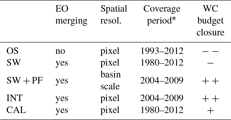
Table 3 Main characteristics of the five merging methods in this study: EO stands for Earth observation satellite datasets, and ^* means not considering the GRACE period coverage. The last column shows the capability of the methodology to close the WC budget. “− −” means bad closure, “−” means quite bad closure, “+” means quite good closure and “+ +” means good closure.

3.5 CALibration (CAL)

To obtain the INT solution, many EO datasets were combined: multiple datasets for each water component (the SW part), and for the various WC components (the PF part). However, if one of the datasets is missing, the INT solution cannot be estimated and this will result in a gap in the time record, and shorter time series of the integrated database.

In Munier et al. (2014), a “Closure Correction Model” (CCM) was introduced to correct each dataset independently, based on the results of the SW + PF integration. The CCM is defined as a simple linear transformation with a scaling factor a and an offset b, such that ${\mathit{X}}_{\mathrm{cal}}=a\cdot {\mathit{X}}_{\mathrm{obs}}+b$. The CCM parameters a and b were calibrated by computing a linear regression between the original observation datasets and the SW + PF components.

A similar approach can be used, with the INT solution as a reference instead of the SW + PF. Instead of calibrating the original EO datasets using basin-scale data, we propose here to calibrate the SW solution towards the INT solution at the pixel scale. This calibration of the SW allows a long-term dataset at the pixel scale to be obtained (see Table 3) with WC budget closure statistics closer to the INT solution. In our tests (not shown), the linear regression is quite satisfactory for the calibration, and it is not necessary to use a more complex statistical regression tool such as a neural network.

The merging/integration techniques used in this study are described in Table 3.

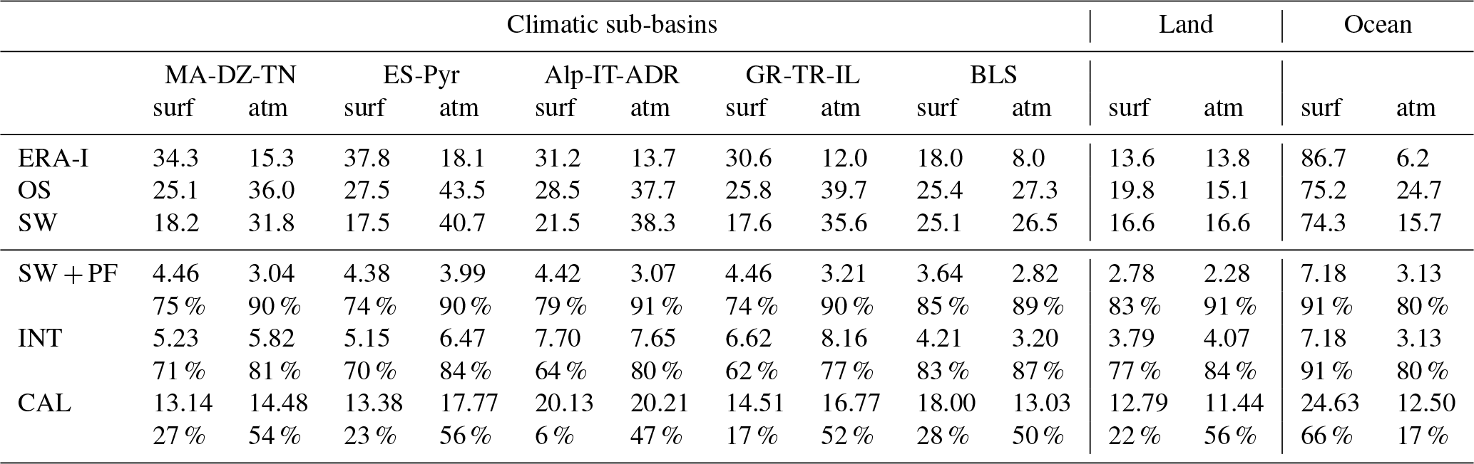
Table 4 rms of the WC budget residual (in mm month⁻¹) over the sub-basin using OS, SW, SW + PF, INT and CAL solutions and for the period 2004–2009. Percentage of improvement of the rms of the residuals from the SW solution to constrained methods is also shown. For comparison purposes, the result using the ERA-I dataset is also depicted.

4 Evaluation of the integrated datasets

In this section, the obtained integrated datasets are first evaluated in terms of WC budget closure. Our EO dataset integration technique is based on the closure of the WC budget. This is a physical constraint, but in some cases (e.g., missing important water component), this constraint could result in a degraded estimation of the components. Therefore, available in situ data (precipitation, evapotranspiration and seawater level) are used to validate some of the water components of the integrated dataset. This evaluation is performed at two different spatial scales: the sub-basin scale and the pixel scale.

4.1 Water cycle budget closure

The residuals of the surface and atmospheric WC budgets for the Mediterranean region are computed at the monthly scale, over the 2004–2009 period. The root mean square (rms) statistics of these residuals are summarized in Table 4 for the six considered products (ERA-I, OS, SW, SW + PF, INT and CAL). Percentages of improvement of the rms of the residuals with respect to the SW solution are also shown for comparison purposes.

ERA-I provides the reanalysis product for all the variables except for the water storage and the discharge, to keep the comparison consistent. It should be noted that ERA-I does not have any water conservation constraint. The optimal selection is given by TMPA precipitation; GLEAM evapotranspiration and OAFlux evaporation; GRGS water storage change over land and JPL water storage change over sea; GPCC-forced ORCHIDEE-CEFREM discharge; and the derivate Globvapor for atmospheric water vapor change. Only one dataset is available for the moisture divergence (Pellet et al., 2017). As shown in Aires (2014), Munier et al. (2014) and Pellet et al. (2017), the SW merging procedure reduces the WC budget residuals at the sub-basin scale, by reducing the random errors of the EO data. The SW product outperforms the ERA-I reanalysis and the OS product. However, the full closure is generally still not satisfactory with this technique. The SW + PF procedure closes the water budget over all the sub-basins, and over the surface and in the atmosphere, with an rms of the residual of about 4 mm month⁻¹. The surface budget residuals are drastically reduced: from 72 % over the GR-TR-IL sub-basin and up to 94 % for the Mediterranean Sea. This shows the necessity to use a WC budget closure constraint that links the six water components.

The INT product provides satisfactory budget closure results (from 61 % to 94 %), even if they are slightly degraded compared to the SW + PF (due to the interpolation process between sub-basins). Since no interpolation has been applied over the Mediterranean Sea, the statistics are equal to the SW + PF.

The CAL product improves the WC budget residuals less compared to INT. Nevertheless, the rms of the residuals for these products is reduced over all sub-basins compared to the SW solution.

Figure A1 gives, in the Appendix, the 2004–2009 time series of all the water component estimates for the various methodologies (SW, SW + PF, INT and CAL) over the various sub-basins as well as the probability density function of the residuals. This figure shows how the WC closure impacts the time series.

4.2 Evaluation at the sub-basin scale

Since the WC budget closure constraint was imposed at the sub-basin scale (see Sect. 3), the evaluation of the integrated product is done at this scale too. Two metrics are used here, the rms of the difference (rmsd) with in situ measurements and the CORRelation (CORR). Only multiple-EO integrated datasets are compared in the two following sections.

Terrestrial precipitation – Table 5 provides the comparison of the EOBS gridded gauge precipitation dataset (Sect. 2.2) with the SW, SW + PF, INT and CAL solutions, in terms of temporal correlation (at the monthly and sub-basin scales), and rmsd, for each sub-basin and for the continental scale (land included in Fig. 1). Since the SW + PF product is defined only on the Mediterranean drainage sub-basins, no statistics are shown for this approach over the continental region (last column). For the rmsd error statistics, results are also provided as improvements compared to the SW solution.

Table 5 Comparison of the SW, SW + PF, INT and CAL precipitation solutions with the EOBS dataset, in terms of correlations, rmsd, and percentage of improvement of the rmsd compared to the SW solution.

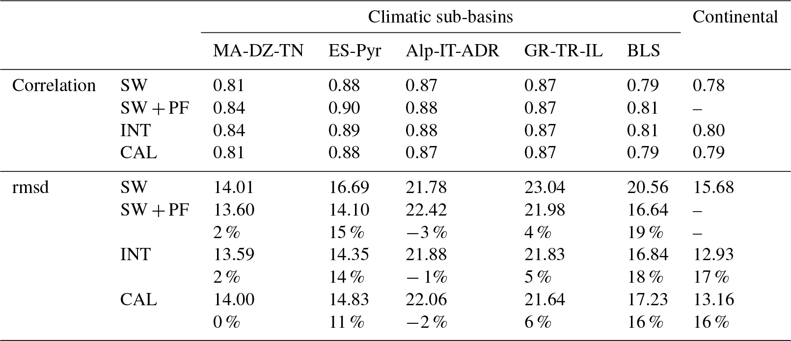
Over all the sub-basins, the SW + PF methodology improves results compared to the unconstrained SW method. Even if the correlation of SW with EOBS is already good, the closure constraint improves this correlation to 0.84 (from 0.81) over the MA-DZ-TN sub-basin. This is true even over the complex sub-basins such as Alp-IT-ADR. SW + PF also reduces the rmsd with EOBS (by up to 20 %). These results show the positive effect of the closure constraint on precipitation. Without explicitly constraining satellite precipitation products towards the in situ data, SW + PF statistics are still improved.

The INT product shows similar CORR and rmsd statistics as SW + PF over the Mediterranean sub-basins, with a slight decrease in the CORR with EOBS over the ES-Pyr sub-basin. Over the continental region, INT improves the correlation compared to SW (from 0.78 to 0.80) while reducing by 17 % the rmsd. Therefore, the interpolation process between the sub-basins (see the spatialization in Sect. 3.4) does not degrade the solution inside the sub-basins, while the extrapolation outside of them improves the unconstrained SW statistics over the whole continent. This is a true benefit since INT presents comparable performances with the SW + PF in terms of closure capability and closeness to in situ measurements, with the advantage of the spatial variability at the pixel scale.

Finally, the CAL precipitation product shows results as good as SW (slightly better for the whole continental region) for the CORR, and smaller rmsd with EOBS. The CAL product does not close the WC budget as well as the INT solution, but it has the advantage of being available over a longer time record (1980–2012) compared to the 2004–2009 INT period.

Seawater-level change – the seawater storage (related to the seawater level) change over the Mediterranean Sea (excluding the Black Sea) is tested using altimetry and thermal datasets over the 2004–2009 period. First, the thermal content estimates of the four datasets presented in Sect. 2.2 are merged into one single estimate. The merged thermal content estimate is then subtracted from the AVISO altimetry seawater level. The monthly change is then computed using the same derivative filter as the one used for GRACE: [5∕24 3∕8 $-\mathrm{3}/\mathrm{8}$ $-\mathrm{5}/\mathrm{24}$].

Figure 3 shows the altimetry estimate and the various methodologies estimates. Since the Mediterranean Sea is considered without the Black Sea for this evaluation, there is no SW + PF estimate (that added the Mediterranean Sea and the Black Sea). While the SW solution has a 0.52 CORR and a 12.2 mm month⁻¹ rmsd with respect to the altimetry estimate, INT statistic are 0.58 for the CORR and 11.8 mm month⁻¹ for the rmsd, and CAL 0.56 for the CORR and 11.8 mm month⁻¹ for the rmsd. Here again, the INT estimate outperforms the unconstrained SW methodology in both CORR and rmsd. CAL presents also better results than SW but the CORR with altimetry is slightly reduced compared to INT. No inter/extrapolation has been used in INT for the “Mediterranean Sea plus the Black Sea” sub-basin and the improvement of INT versus SW is due only to the impact of the closure constraint. Nevertheless, the SW + PF approach closes the WC over the Mediterranean Sea within the Black Sea (no information about the Bosporus netflow) and the spatial downscaling in INT is needed to discriminate the closure correction above the two seas. Using the WC closure over the Mediterranean and Black Sea improves the water storage change estimates.

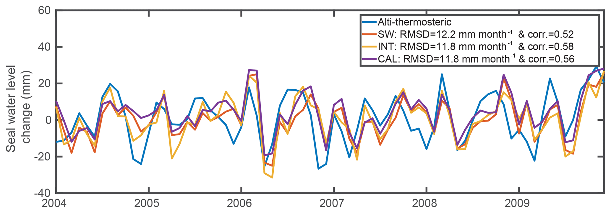
Figure 3 Seawater-level evaluation of SW, INT and CAL estimates compared to altimetry minus thermal content. The correlation difference is statistically significant at the 70 % level based on the T-test.

4.3 Evaluation at the pixel scale

The INT and CAL estimates are here evaluated at the pixel scale, for precipitation and evapotranspiration. Improvements of SW by INT and CAL are measured using in situ measurements of precipitation and evapotranspiration from the FLUXnet database, available over the Mediterranean region, for the 2004–2009 period (Sect. 2.2).

Figure 4 presents the scatterplots of the rmsd between the SW estimate (E_SW) and INT or CAL (E_cor for “corrected”) datasets with the FLUXnet evapotranspiration data (E_FLUX), for each station. The 1:1 line is also shown. Each dot under the 1:1 line represents an improvement at the corresponding station from SW solution to INT and/or CAL. INT and CAL improve evapotranspiration estimates for more than 53 % of the sites. The distribution of the differences in the encapsulated figure is slightly narrowed by the INT and CAL compared to the SW solution. Location of the station where the closure improves the rmsd with the flux measurement is shown in green if INT and CAL both improve the estimate, blue when only CAL improves, and magenta when only INT improves. Red dots represent stations where there is a degradation in both INT and CAL. The evaluation of the EO estimate at 0.25^∘ spatial resolution using tower sites should be made with caution. The poor performance of satellite estimates over particularly complex topography (mountainous rainfall) or coastal pixels with land–sea contamination could explain the difference between the INT estimate and the FLUXNET measurement on these particular locations.

Figure 5 presents the scatterplots of the rmsd between the SW estimate (P_SW) and the INT or CAL (P_cor) datasets with the FLUXnet precipitation data (P_FLUX), for each station. Over most stations (82 %), the INT and CAL solutions improve the precipitation estimate compared to SW. Locations of improved sites are shown with the same color code as in Fig. 4. It can be seen in Fig. 5 that red dots are located mainly in mountainous or coastal regions. These two types of landscape are really challenging for precipitation retrieval due to snow precipitation on the one hand and coastal sea–land contamination on the other.

5 A coherent multi-component dataset for the water cycle monitoring

In this section, the integrated datasets are used to deliver updated estimates of the Mediterranean WC budget. The impact of hydrological constraint (PF) as well as the INTegration (INT) and CALibration (CAL) processes on the spatial averaging of the water component estimates and the WC budget residuals, over the several Mediterranean sub-basins, is summarized in Fig. A1 of the Appendix.

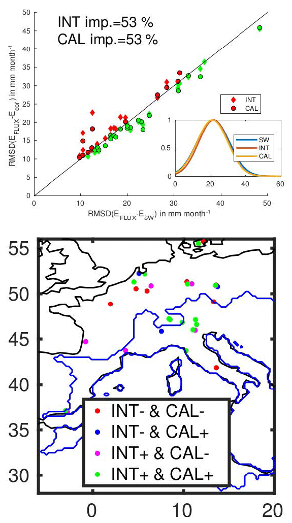
Figure 4 Top panel: scatterplot of the rmsd between FLUXnet station and the SW, INT and CAL products, for evapotranspiration. Dots under the 1:1 line (green) show improvement, and dots over the line (red) show degradation. INT and CAL results are superposed for some locations, meaning that the linear approximation in CAL is enough to mimic the INT scaling factors at these location. The encapsulated figure shows the distribution of the differences with the Fluxnet estimates. Bottom panel: location of the FLUXnet stations used for validation: green dots show an improvement for INT and CAL compared to SW (INT+ and CAL+), blue dots show improvement only for CAL (INT− and CAL+), and magenta only for INT (INT+ and CAL−). Red dots is where no improvement is observed (INT− and CAL−). Blue line limits the total basin area.

5.1 Analysis of the Mediterranean WC

The mean fluxes of the Mediterranean WC and associated variability over the 2004–2009 period are depicted in Fig. 6. The WC is analyzed over its natural sub-basin boundaries. The variability is computed as the standard deviation of the annual values over the period. These values have been computed over the respective terrestrial or oceanic sub-basins, considering all the drainage area in western Europe and BLS or in Africa within Turkish coastal region but without considering the Nile River basin (for which just its discharge is represented), Black Sea or Mediterranean Sea. The large font corresponds to the INT, and the little font is for SW. The two values for the netflow estimate at the Bosporus Strait are estimated as the deficit term of the water budget equation, computed over the Mediterranean and the Black Sea independently. Using INT estimates (i.e., closure of the two seas at once), the two values are in better agreement with each other than with the two SW estimates. In the following, only the INT values are described.

Figure 5 Same as Fig. 4 but for precipitation.

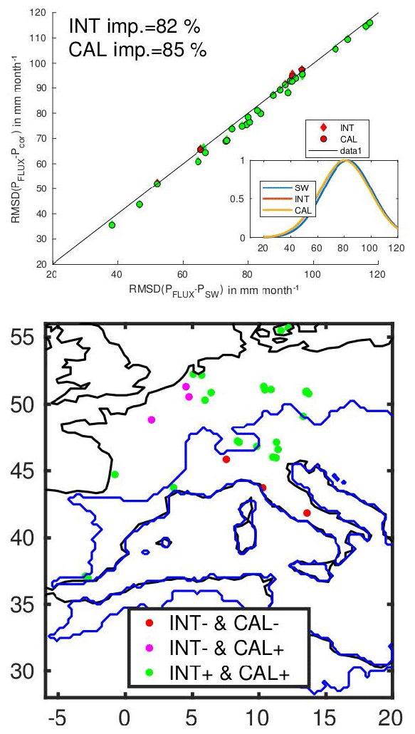
Figure 6 shows the uneven water contribution between the European (314±57 km³ yr⁻¹ for the total discharge) and the African (21±30 km³ yr⁻¹) drainage area to the Mediterranean Sea budget. Furthermore, it shows the role of the Black Sea in the global Mediterranean WC. Most of the European freshwater flows to the BLS (398±70 km³ yr⁻¹; it represents more than 50 % of the European discharge), where the E−P balance allows for an equal contribution to the Mediterranean Sea budget though the Bosporus Strait input. Considering the Nile discharge, the closure optimization increase the discharge value (from 19±6 to 76±30 km³ yr⁻¹). Recent discussions on the Nile discharge can be found in Jordà et al. (2017). Our new discharge estimates include the groundwater discharge passing through the aquifers.

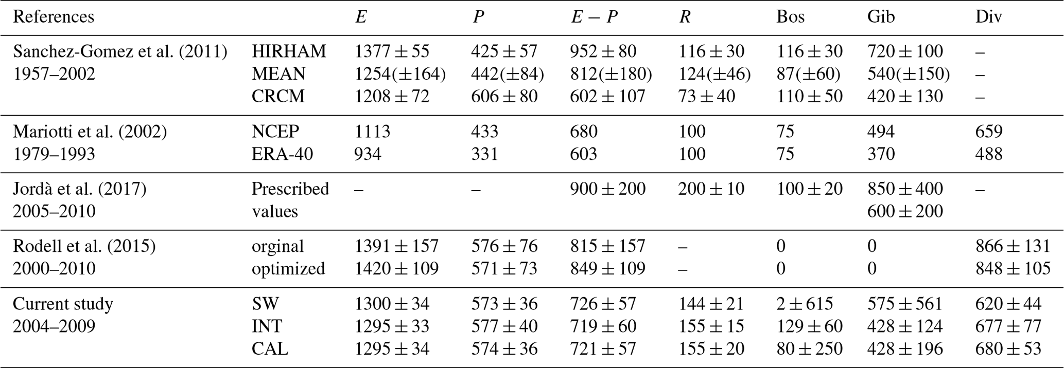
Sanchez-Gomez et al. (2011)Mariotti et al. (2002)Jordà et al. (2017)Rodell et al. (2015)

Table 6 Comparison in the literature for the Mediterranean Sea (without the Black Sea) average annual mean fluxes and their associated variability (in mm yr⁻¹). While the variability of the real product is computed as the standard deviation of annual values, the uncertainty associated with the regional climate models' mean is the inter-model spread. The periods of analysis for the various studies are recalled.

After closure optimization, the annual precipitation, evapotranspiration and moisture divergence over the European drainage area are estimated to be 770±40, 510±10 and 77±60 km³ yr⁻¹, respectively. Europe accumulates most of the moisture coming from the Mediterranean Sea (1787±200 km³ yr⁻¹), while the Black Sea poorly evacuates its moisture towards land (91±60 km³ yr⁻¹). Over land the contribution of the African part to the global moisture divergence is quite high (274±43 km³ yr⁻¹ mainly due to the presence of the Atlas mountains). The two netflow estimates at the Bosporus Strait are very close, with a difference lower than its associated uncertainty in Fig. 6. Freshwater inputs at the two Mediterranean straits (Bosporus and Gibraltar) compensate for the very large evaporation loss (3372±88 km³ yr⁻¹) of the Mediterranean Sea. This process represents more than twice the precipitation (1499±102 km³ yr⁻¹).

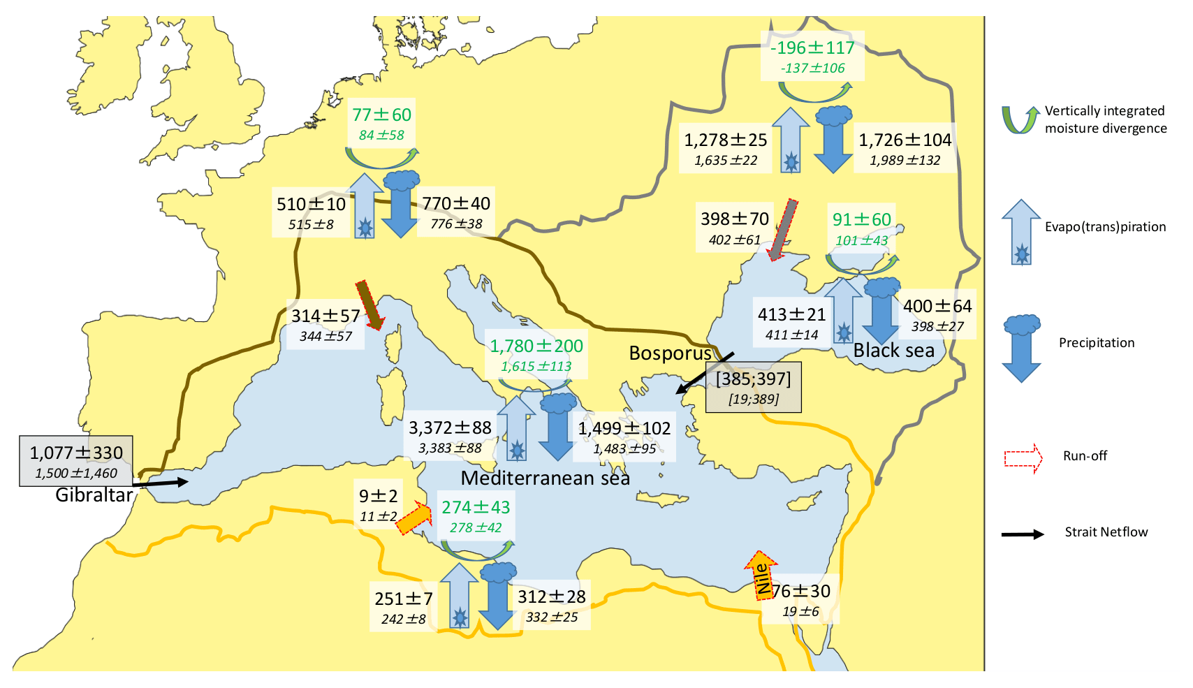
Figure 6 Mean annual fluxes (km³ yr⁻¹) of the Mediterranean WC and associated uncertainties in SW (small font) and INT (large font) during the 2004–2009 period.

Figure 6 represents the whole WC over the considered region with its main features: the role of the Mediterranean Sea as the moisture and energy reservoir for the surrounding land; the poor contribution of the African coasts in terms of water resource, and the role of the Black Sea as the buffer process for the freshwater input. This quasi-triangular process emphasizes the hydrological link between the surrounding land and the two seas.

5.2 Comparison of the Mediterranean flux estimates with the literature

Table 6 summarizes the comparison of the various estimates of the water fluxes in the current analysis with what can be found in the literature. The various annual mean estimates are based on different time periods and comparison must be taken with caution since some interannual variability is likely to be due to the change in hydrologic regime. Sanchez-Gomez et al. (2011) focused on the Mediterranean Sea heat and water budget using an ensemble of ERA-40-driven high resolution Regional Climate Models (RCMs) from the FP6-EU ENSEMBLE database. The atmospheric budget was not considered in Sanchez-Gomez et al. (2011) and no moisture divergence estimate was provided. For comparison purposes, we decided to select the RCM ensemble-mean estimate and two particular models: the Danish HIRHAM (Hesselbjerg Christensen and Meteorologisk Institut, 1996) and the Canadian CRCM (Plummer et al., 2006). These two models have been selected since their E−P estimates are the extremes of the RCMs ensemble. In Sanchez-Gomez et al. (2011), the netflow at Gibraltar was estimated as the deficit term of the WC: $\mathrm{Gib}=E-P-R-\mathrm{Bos}$.

Mariotti et al. (2002) analyzed the WC over the Mediterranean region in the context of the NAO teleconnection over the 1979–1993 period using two reanalyses (ERA-40 and NCEP-NCAR) for precipitation, evaporation and moisture divergence. They used the discharge data from the monitored rivers through the Mediterranean Hydrological Cycle Observing System (MED-HYCOS) and GRDC. Their estimate includes a total Mediterranean input of 100 mm yr⁻¹ from MED-HYCOS and the Bosporus input of 75 mm yr⁻¹ from the literature (Lacombe and Tchernia, 1972). Mariotti et al. (2002) estimated the netflow at Gibraltar as the balance of the Mediterranean water deficit using the equation $\mathrm{Gib}=\mathrm{Div}-R-\mathrm{Bos}$ coming from the oceanic and atmospheric budgets and the null assumptions about the storage change. Mariotti et al. (2002) used old versions of the reanalyses and some remarks have already been made on the precipitation and evapotranspiration estimates for these versions. Nevertheless, to our knowledge, Mariotti et al. (2002) was the last effort to estimate the atmosphere WC over the Mediterranean.

Jordà et al. (2017) reviewed the state-of-the-art in the quantification of the various water component estimates. Their estimates presented in Table 6 are the best consensual values among the scientific community. They are based on several studies and take into account the results of Mariotti et al. (2002) and Sanchez-Gomez et al. (2011) for example. In particular, the mean Gibraltar netflow estimate from Jordà et al. (2016) has been commented on and the new mean is provided in Jordà et al. (2017).

Table 6 also shows the results from Rodell et al. (2015) before and after their satellite data optimization based on a variational assimilation at the annual scale. The constraints of the fluxes over the Mediterranean Sea and the Black Sea were made independently (considering no netflow at the Bosporus Strait). The Mediterranean Sea was closed with no exchange to the Atlantic at Gibraltar (no netflow). Rodell et al. (2015) provided no explicit discharge for the Mediterranean Sea, but only for the Eurasian continent.

For the four mentioned articles, only the Mediterranean Sea without the Black Sea is considered. No estimate from SW + PF methodology is provided in Table 6. Our integrated dataset is the only one to use direct observations for the Gibraltar netflow and to compute the Bosporus netflow via a WC budget. For all estimates, Table 6 presents their associated variability. While the variability of real products is computed as the standard deviation of the annual values, the variability associated with the RCM mean is the inter-model spread (i.e., proxy of the uncertainty).

Evaporation – the RCM ensemble mean for the annual evaporation is 1254 mm yr⁻¹ with an inter-model spread of 164 mm.yr⁻¹. Some RCMs evaluated higher annual evaporation, as the HIRHAM model that estimated 1377±55 mm yr⁻¹. On the contrary, Mariotti et al. (2002) found a lower evaporation with the reanalyses (1113 and 934 mm yr⁻¹ for NCEP and ERA). Rodell et al. (2015) estimated much higher evaporation and higher annual variability with an mean annual value of 1391±157 mm yr⁻¹ using only OAFlux and 1420±109 mm yr⁻¹ after optimization. Our unconstrained SW solution gives an annual value of 1300±34 mm yr⁻¹ and our constrained INT product gives 1295±33 mm yr⁻¹. The CAL estimate is close to the INT solution.

Precipitation – the RCM ensemble mean for the annual precipitation was 442±84 mm yr⁻¹ which is quite close to the NCEP reanalyses value in Mariotti et al. (2002). Satellite estimates in both Rodell et al. (2015) and the current study indicate higher precipitation: 576 and 571 mm yr⁻¹ in Rodell et al. (2015) and from 573 to 577 mm yr⁻¹ after the closure constraint in this work. SW, INT and CAL products present similar precipitation estimates at the annual scale due to the quite low uncertainty associated with the precipitation in the integration. Even if the spread among the RCMs was lower than for the evaporation, some RCMs such as CRCM did compute even larger precipitation than what has been retrieved from satellites (606±80 mm yr⁻¹). Sanchez-Gomez et al. (2011) had already noted that gauges-calibrated satellite datasets such as GPCP and TMPA tend to have higher precipitation values than what was simulated in the RCMs. Precipitation over the Sea is a sensitive variable and its validation is difficult due to the lack of buoys. The ERA reanalyses value in Mariotti et al. (2002) was low compared with the NCEP estimate.

Evaporation minus precipitation – Sanchez-Gomez et al. (2011) focused on E−P to assess the physical consistency in the RCMs. They assumed that a model with high evaporation tends to have higher precipitation. The averaged E−P budget among the RCMs was 812±180 mm yr⁻¹ and the range was between 952±80 (HIRHAM model) and 602±107 mm yr⁻¹ (CRCM model). The inter-model spread was high for the E−P budget, stressing the difficulties in providing realistic water budget evaluation. Rodell et al. (2015) found a similar E−P budget, but the associated variability was high too due to the uncertainty in evaporation. Our E−P estimates are, respectively, 726±57 and 719±60 mm yr⁻¹ before and after the closure constraint. These values are lower but still in the RCM ensemble range. They are closer to what Mariotti et al. (2002) found with NCEP reanalyses. Jordà et al. (2017) consider the net surface flux to be 900±200 mm yr⁻¹, which is in good agreement with the CRCM model estimate. Rodell et al. (2015) found a similar E−P budget but with far higher evaporation estimates, which seemed quite unrealistic. Furthermore, their closure constraint tends to increase the evaporation value and then the E−P budget.

Discharge – only the RCMs providing the runoff have been used to compute the annual value of R (124±46 mm yr⁻¹) in Sanchez-Gomez et al. (2011). Mariotti et al. (2002) found comparable values for the discharge, considering only the monitored rivers. Rodell et al. (2015) did not include explicit discharge into the Mediterranean Sea since the closure was done at the global scale (Eurasian continent) and no value was provided for the Mediterranean freshwater input. Our discharge estimate is increased from 144±21 in SW to 155±15 mm yr⁻¹ in INT after the optimization. This increase is mainly driven by the re-evaluation of the Nile discharge that present larger discharge (76 km³ yr⁻¹) after closure. All these discharge estimates are lower than the value prescribed in Jordà et al. (2017) (200±10 mm yr⁻¹).

Black Sea discharge – the RCM ensemble-mean value for the freshwater input through the Bosporus Strait was 87±60 mm yr⁻¹, stressing the high discrepancies among the RCMs. Rodell et al. (2015) closed independently the Mediterranean and Black seas, with no exchange between the two oceanic basins (i.e., the netflow equals zero). In the current approach, the Black Sea discharge is computed as the deficit in the water budget for the Mediterranean Sea, by considering the netflow at Gibraltar (Gib) corrected from Jordà et al. (2016): $\mathrm{Bos}=E-P-R-\mathrm{Gib}$. The SW product presents an unrealistic value for the Black Sea discharge (2.0±615 mm yr⁻¹); this is mainly due to the high uncertainty associated with the netflow at Gibraltar. On the other hand, the closure constraint improves the Bosporus netflow estimate, which equals 129±60 mm yr⁻¹ with INT after optimization. The value is close to the deficit of the Black Sea water budget (computed after optimization), 132±60 mm yr⁻¹ (not shown in Table 6), stressing the consistency between the two seas' water budget. The value is still higher than the estimate of 75 mm yr⁻¹ in Mariotti et al. (2002).

Gibraltar netflow – Rodell et al. (2015) considered no flow at Gibraltar when closing the Mediterranean WC and then provided no estimate for this variable. Both Sanchez-Gomez et al. (2011) and Mariotti et al. (2002) evaluated the netflow by closing the WC over the Mediterranean region but they used different assumptions and equations. The estimate in Sanchez-Gomez et al. (2011) is based on the oceanic closure while it is based on both the oceanic and atmospheric closure in Mariotti et al. (2002). The RCM ensemble mean was 540±150 mm yr⁻¹ in Sanchez-Gomez et al. (2011), while Mariotti et al. (2002) found lower value with the reanalyses (493 and 370 mm yr⁻¹ with NCEP and ERA). Jordà et al. (2017) give two values for the netflow at Gibraltar: one from direct observations but suffering from large uncertainties (850±400 mm yr⁻¹), and the other as the deficit of the water budget (600±200 mm yr⁻¹). The value in INT and CAL estimate are impacted by the closure constraint. The netflow estimate after optimization (428±124 mm yr⁻¹) is lower than what can be found in Jordà et al. (2017) but in the range of the RCMs water budget deficit.

textitMoisture divergence – no moisture divergence was provided by the RCMs in Sanchez-Gomez et al. (2011). Mariotti et al. (2002) found moisture divergence to be 659 mm yr⁻¹ in NCEP and 488 mm yr⁻¹ in ERA. Rodell et al. (2015) estimated the divergence to be 848±105 mm yr⁻¹ after optimization. The difference between Rodell et al. (2015) and Mariotti et al. (2002) estimates and what is found in the current study is mainly driven by the discrepancy between the three reanalyses: Modern-Era Retrospective Analysis for ReSearch and Applications (MERRA) used by Rodell et al. (2015), NCEP and ERA-40 by Mariotti et al. (2002), and ERA-I used in the current analysis. Recent works focusing on atmospheric reanalyses comparisons have demonstrated the ERA-I quality. Stopa and Cheung (2014) have stressed the ERA-I performances in the representation of long term wind variability, critical for the representation of moisture divergence. Brown and Kummerow (2013) have pointed out that satellite derived E−P (SeaFlux-GPCP) correlates well with ERA-Interim atmospheric moisture divergence. Trenberth et al. (2011) have assessed the performance of ERA-I reanalysis for atmospheric moisture budgets consideration.

6 Conclusions

The main goal of this work was to build a multi-component dataset describing the Mediterranean hydrology by constraining the WC closure. Various methodologies have been presented and particular attention has been placed on the INTegration method. This approach fulfills the previously stated objectives: being a pixel-wise dataset but in which the WC closure is controlled. INT is an integrated dataset that shows several benefits compared to previous studies. The INT product allows reduction of the rms of the WC budget residual down to 3.55 mm month⁻¹ over land and 5.27 mm month⁻¹ in the atmosphere. These reductions represent an improvement of, respectively, 78 % and 80 % compared to the best unconstrained satellite combination dataset. The temporal coverage of INT is limited by the common coverage period 2004–2009 of all the satellite estimates used in this study (see Table A2).

The INT dataset has been evaluated at various scales. Even if the evaluation is a difficult task and the presented work is not exhaustive, our results show that the consideration of the WC closure allows one to reduce differences with the available in situ measurements. At the sub-basin scale, the overall precipitation is closer to the in situ gridded EOBS dataset after being constrained. The seawater-level estimate is also improved compared to the altimetry estimate. At the pixel scale, the INT estimate shows a better agreement with in situ tower measurements from the FLUXnet2015 database.

The WC has been analyzed in terms of long-term means over the 2004–2009 period and compared with the previous literature. The INT methodology has improved estimates of the Mediterranean water components. The INT product provides more realistic values for both the Bosporus and Gibraltar netflows by constraining them with the satellite observations. Note that the Bosporus estimate is mainly driven by the Gibraltar estimate and can then be improved if the Gibraltar netflow evaluation would become more accurate.

This study conducted on the Mediterranean Sea is innovative from previous work. The Mediterranean WC has already been well investigated by Mariotti et al. (2002) and Sanchez-Gomez et al. (2011) relying on models and reanalyses. At the global scale, Rodell et al. (2015) close independently the Mediterranean and Black seas using satellite observations, while Sanchez-Gomez et al. (2011) close the Mediterranean Sea WC in estimating the Gibraltar netflow as the WC budget deficit. This study aims to provide a full description of the WC, based on fewer hypotheses. It is the first effort to close the WC at the surface and in the atmosphere over the whole Mediterranean region, using satellite observations and in situ measurement for the Gibraltar netflow.

There are still large uncertainties in the WC components, but the INT methodology appears to be a valuable approach, in particular to include coherency among these components. The current work has also introduced the CAL product which is a calibration of the satellite products that can be used to extrapolate in time the closure constraint. The CAL product is less efficient in closing the WC, but presents the advantage of having longer temporal coverage. Several improvements will be considered in the future: (1) more accurate in situ observations (e.g., Bosporus netflow estimate or coastal discharges) should lead to improved estimates. (2) New WC inputs could be considered (e.g., groundwater exchange or horizontal exchange at the oceanic sub-basin scale) to better characterize the flux and stock terms in the WC. (3) The use of other sources of EO estimates should be considered. For example, the evapotranspiration estimate based on the closure of the energy cycle (Su, 2002; Chen et al., 2013) could be tested. This dataset could be an opportunity to (4) close simultaneously the water and the energy cycles and should lead to a better estimate of the evapotranspiration over land. Multiple-component dataset INT shows promising aspects for forcing, calibrating or constraining regional models with a water conservation constraint. Some developments and evaluations are still required before the production of a climate data record (Su et al., 2018) can be started. The two databases (INT and CAL) can however be obtained under request to the corresponding author or via the HyMeX data server (http://mistrals.sedoo.fr/HyMeX/, last access: 24 January 2019).

Appendix A

Figure A1 compares the six water component estimates and the pdf of the two WC budget errors. The estimates are for the six terrestrial sub-basins, the oceanic part and the total land (in column) through the various methodologies presented in the study: SW, SW + PF, INT and CAL. The figures show by how much the water budget residuals are reduced and how the water components are impacted.

Table A1 gathers the notation used in the study.

Table A2 lists the datasets used in the study.

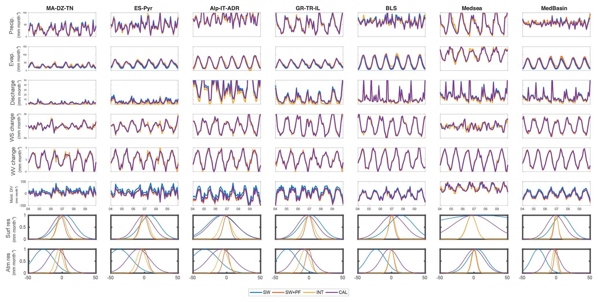
Figure A1 Comparison of the six water component estimates and the pdf of the two WC budget errors (in row). The estimates are for the six terrestrial sub-basins, the oceanic part and the total land (in column) through the various methodologies presented in the study: SW, SW + PF, INT and CAL.

Table A1 Notation used in this study.

Adler et al. (2003)Joyce et al. (2004)Huffman et al. (2007)Ashouri et al. (2015)Dee et al. (2011)Haylock et al. (2008)Falge et al. (2017)Martens et al. (2017)Mu et al. (2011)Zhang et al. (2010)Dee et al. (2011)Falge et al. (2017)Sun et al. (2003)Curry et al. (2004)Dee et al. (2011)Bettadpur (2012)Dahle et al. (2013)Biancale et al. (2005)Watkins and Yuan (2014)Watkins et al. (2015)Schneider et al. (2013)Dee et al. (2011)Ludwig et al. (2009)Polcher et al. (1998)Dee et al. (2011)Jordà et al. (2016)

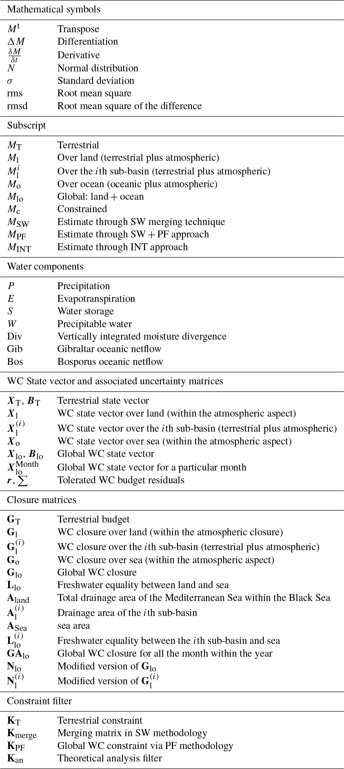
Table A2 Overview of the various datasets used in this study. Their common coverage period, on which the WC budget is estimated, is 2004–2009.