the Creative Commons Attribution 4.0 License.
the Creative Commons Attribution 4.0 License.
 | 18 Nov 2019
High-resolution regional climate modeling and projection over western Canada using a weather research forecasting model with a pseudo-global warming approach
Zhe Zhang
Liang Chen
Sopan Kurkute
Lucia Scaff
Xicai Pan
Climate change poses great risks to western Canada's ecosystem and socioeconomical development. To assess these hydroclimatic risks under high-end emission scenario RCP8.5, this study used the Weather Research Forecasting (WRF) model at a convection-permitting (CP) 4 km resolution to dynamically downscale the mean projection of a 19-member CMIP5 ensemble by the end of the 21st century. The CP simulations include a retrospective simulation (CTL, 2000–2015) for verification forced by ERA-Interim and a pseudo-global warming (PGW) for climate change projection forced with climate change forcing (2071–2100 to 1976–2005) from CMIP5 ensemble added on ERA-Interim. The retrospective WRF-CTL's surface air temperature simulation was evaluated against Canadian daily analysis ANUSPLIN, showing good agreements in the geographical distribution with cold biases east of the Canadian Rockies, especially in spring. WRF-CTL captures the main pattern of observed precipitation distribution from CaPA and ANUSPLIN but shows a wet bias near the British Columbia coast in winter and over the immediate region on the lee side of the Canadian Rockies. The WRF-PGW simulation shows significant warming relative to CTL, especially over the polar region in the northeast during the cold season, and in daily minimum temperature. Precipitation changes in PGW over CTL vary with the seasons: in spring and late autumn precipitation increases in most areas, whereas in summer in the Saskatchewan River basin and southern Canadian Prairies, the precipitation change is negligible or decreased slightly. With almost no increase in precipitation and much more evapotranspiration in the future, the water availability during the growing season will be challenging for the Canadian Prairies. The WRF-PGW projected warming is less than that by the CMIP5 ensemble in all seasons. The CMIP5 ensemble projects a 10 %–20 % decrease in summer precipitation over the Canadian Prairies and generally agrees with WRF-PGW except for regions with significant terrain. This difference may be due to the much higher resolution of WRF being able to more faithfully represent small-scale summer convection and orographic lifting due to steep terrain. WRF-PGW shows an increase in high-intensity precipitation events and shifts the distribution of precipitation events toward more extremely intensive events in all seasons. Due to this shift in precipitation intensity to the higher end in the PGW simulation, the seemingly moderate increase in the total amount of precipitation in summer east of the Canadian Rockies may underestimate the increase in flooding risk and water shortage for agriculture. The change in the probability distribution of precipitation intensity also calls for innovative bias-correction methods to be developed for the application of the dataset when bias correction is required. High-quality meteorological observation over the region is needed for both forcing high-resolution climate simulation and conducting verification. The high-resolution downscaled climate simulations provide abundant opportunities both for investigating local-scale atmospheric dynamics and for studying climate impacts on hydrology, agriculture, and ecosystems.
- Article
(22260 KB) - Full-text XML
-
Supplement
(19214 KB) - BibTeX
- EndNote


Climate change has been increasingly evident, as shown by the rising global mean surface temperature since the instrumental records started in the 19th century (Bindoff et al., 2013; IPCC, 2013). Climate change and its potential risks to the environment and society have become one of the most pressing issues for humanity. As greenhouse gas (GHG) emissions continue to rise due to human activities in the foreseeable future, the global mean temperature will increase, consequently, so will climate extremes (Easterling et al., 2000; Karl et al., 2006; Sugiyama et al., 2009). The changing climatological mean and increasing extremes could impact many aspects of the ecosystem, environment, and society. Although consensus about climate change has been established, how the regional climate systems will respond to potential GHG radiative forcing is less clear due to the complexity of the climate system and uncertainties in future emissions. Even for a specific representative concentration pathway, it is unclear how the regional climate and hydrology will respond. This challenge to project a regional climate response is due not only to the complexity of atmosphere, ocean, land surface, and hydrological processes themselves, but also to the numerous interconnections, interactions, and types of feedback between each component of the climate system.
Numerical models, supported by comprehensive observation validations, are indispensable tools to enhance our knowledge of the climate system and to make climate projections. Global climate models (GCMs) have been widely used to assess the climatic impacts of accumulated GHG emissions and to project the future climate under different emission scenarios since the industrial revolution. For example, the Coupled Model Intercomparison Project Phase 5 (CMIP5) comprises more than 20 model centers and more than 60 GCM combinations. CMIP5 uses a standard set of model simulations to evaluate how realistic the GCMs are in simulating the recent past and also provides multiple scenario projections of future climate changes in the near term (out to about 2035) and long term (out to 2100 and beyond).
GCMs include a multitude of processes with a gamut of temporal–spatial scales. To represent the complex climate system in numerical models, processes ranging from scales as small as aerosols and turbulence to those as large as the planet, e.g., the continental drift in paleoclimate simulation, have to be formulated explicitly or through parameterization. To faithfully represent the basic energy balance of the planet, GCMs need to simulate the planetary-scale climate processes that transfer heat and mass through extensive ocean currents and jet streams. In addition to this large-scale advection in the atmosphere and oceans by mean flow, GCMs also need to simulate the atmospheric and oceanic eddies embedded in the flow that transport a massive amount of heat meridionally. These eddies, which rise from the thermal gradient, are bound to evolve as the global temperature rises and alters the tropic–polar thermal gradient. Because of the complexity of the climate system, different approaches to numerically represent the climate processes can introduce substantial inter-model variability among GCMs (Deser et al., 2012; Mearns et al., 2013). Climate projections from GCMs introduce large uncertainties and usually an ensemble mean of GCMs is used to reduce the uncertainty.
The climate system also has multiple-year oscillations (e.g., the El Nino–Southern Oscillation) and multi-decadal oscillations (e.g., the Pacific Decadal Oscillation and Atlantic Meridional Oscillation), which often obscure the secular trend (Xie and Kosaka, 2017). To average out the natural oscillations in the climate system and to reach equilibrium for the slow processes (e.g., deep ocean circulation, permafrost), GCM usually needs to perform simulations for periods from decades to centuries. Due to high computation costs, the large spatial and temporal scales that GCMs have to capture compel them to settle on coarse resolutions. Thus, GCMs have to represent the effects of small-scale processes such as convection, gravity waves, and turbulent transport through parameterization.
However, climate impacts on the ecosystem and human society often occur on local and regional scales, both of which are important for climatic impacts. For example, surface air temperature is strongly affected by underlying surface and local circulation. To bridge the gap between large-scale projection and local-scale climatic impact, regional climate downscaling is often performed on GCM projections. Statistical downscaling has the advantage of being computationally cheap and easy to implement but suffers from the assumption of the stationarity of the statistical distribution of the hydrometeorology variables. In an ever-changing climate and earth system, stationarity is not a norm but an exception. Dynamical downscaling using regional climate models (RCMs) can provide added value to the understanding of regional climate change by explicitly representing some of the small-scale processes that are critical but poorly represented in GCMs (Castro, 2005).
The added values of RCM simulations relative to driving GCMs are widely accepted, especially in regions with a strong heterogeneous underlying boundary and for mesoscale atmospheric processes, in particular, when the RCM is constrained at the large spatial scales through boundary conditions and spectral nudging (Feser et al., 2011). RCM simulations are especially valuable for variables such as near-surface temperature and humidity, which are strongly affected by the representation of near-surface processes. The mesoscale phenomena such as polar lows (Feser et al., 2011) and mesoscale convective systems (Prein et al., 2017a) can be represented more realistically in RCM simulations. Because RCMs can resolve subgrid-scale processes in GCMs, which are important to water cycles and the ecosystem, they are widely used to provide detailed projections of future climate scenarios and downscaling information for impact studies, especially those associated with the aforementioned fine-scale processes.
RCMs have been individually applied to downscale temperature and precipitation projection over North America and under inter-comparison frameworks such as NARCCAP (Mearns et al., 2009, 2015) and CORDEX (Giorgi et al., 2009). These inter-comparison frameworks provide a glimpse into the uncertainties in regional climate downscaling through a common combination of driving GCMs, RCMs, and multiple emission scenarios. The horizontal resolutions of RCMs used in the recent coordinated regional climate downscaling efforts are usually larger than 10 km. With these relatively coarse resolutions, RCMs still have to rely on convection parameterization to represent deep convection in the models.
In climate simulation, convection parameterization is a major source of errors, which is used to represent the statistical effects of subgrid cumulus plumes on the redistribution of mass, heat, and momentum on the grid-scale mean flow. Convection parameterization used in GCMs and coarse-resolution RCMs causes bias in the simulated hydrological cycle: underestimated dry days, misrepresentation of the diurnal cycles of convective precipitation, etc. Deep convection, however, contributes to a relatively large percentage of precipitation amounts and extremes, especially during warm seasons. Poor simulation of deep convection is a stubborn problem for RCMs in climate projection and regional climate dynamical downscaling. One way to avoid the errors introduced by convective parameterization is to resolve convection explicitly with high-resolution models. RCMs with horizontal grid spacing less than 4 km can resolve convective processes and are often referred to as convection-permitting models (CPMs). As well as explicitly representing deep convection, CPMs also permit a more accurate representation of underlying surface and topography. As computing capability grows, CPMs or cloud-resolving models emerge as a promising tool to generate more realistic regional- to local-scale climate simulations compared to models with coarser resolution and convective parameterization (Prein et al., 2015). Although CPMs require higher computational resources than lower-resolution models, the computing costs of CPMs can be justified by their ability to simulate mesoscale convective systems more realistically and to produce better convective and orographic precipitation (Prein et al., 2015; Weusthoff et al., 2010).
CPMs have great benefits for dynamical downscaling over western Canada due to its geographic characteristics. Most notably, western Canada features the Canadian Rockies, where steep terrain and small-scale atmospheric processes play important roles in wave dynamics and mountain meteorology. In cold seasons, especially, the atmosphere, hydrology, and cryosphere strongly couple with each other through small-scale boundary-layer processes, including snow cover, snowmelt, and blowing snow. On the other hand, western Canada also encompasses the Canadian Prairies, where climate downscaling seems straightforward because of its seemingly homogeneous landscape. However, in the Prairies summer convections contribute the most precipitation, and these subgrid-scale convections in GCMs need to be properly simulated by using high-resolution convection-permitting models.
To provide high-resolution convection-permitting downscaling for western Canada, a set of 4 km convection-permitting Weather Research and Forecasting (WRF) simulations was conducted for the current climate and the high-end emission scenario of RCP8.5. The 4 km convection-permitting retrospective simulation (CTL, October 2000–September 2015) was driven by ERA-Interim reanalysis (Dee et al., 2011). The future climate sensitivity simulation was conducted using reanalysis-derived initial and boundary conditions for the same period as CTL but perturbed with changes in field variables derived from the CMIP5 ensemble-mean high-end emission scenario (RCP8.5) climate projections, the so-called pseudo-global warming (PGW) method. In this paper, we evaluate the performance of the retrospective simulation and investigate the dynamically downscaled regional climate change over western Canada, especially the Mackenzie River basin (MRB) and Saskatchewan River basin (SRB). We evaluated the capability of the current generation of RCMs such as WRF, running at convection-permitting resolution to reproduce precipitation and temperature features important for hydrology and water resources applications in western Canada. The paper is organized as follows: Sect. 2 introduces the model setup and data; Sect. 3 evaluates the retrospective simulation (CTL) against observation; Sect. 4 describes the projected climate change by the PGW vs. CTL; Sect. 5 shows the changes in temperature and precipitation extremes; Sect. 6 discusses the results, and Sect. 7 summarizes the results and concludes the paper.
2.1 Model setup
The WRF model Version 3.6.1 was used to simulate the historical (2000–2015) and projected climate (RCP8.5) over western Canada with a convection-permitting resolution of 4 km. The WRF model is fully compressible and nonhydrostatic and uses the Advanced Research WRF (ARW) dynamical solvers. The model domain is composed of 699×639 grid points with 4 km horizontal resolution to cover western Canada from British Columbia and the Yukon to the west and the MRB and the SRB to the east as shown in Fig. 1. In total, the model domain covers 2800 km in the east–west direction and 2560 km in the north–south direction. The model's vertical coordinate comprised 37 stretched vertical levels topped at 50 hPa in the lower stratosphere. The model simulations employed several parameterization schemes, including the Thompson microphysics scheme (Thompson et al., 2008), the Yonsei University (YSU) planetary boundary-layer scheme, the Noah land surface model (Chen and Dudhia, 2001), and the CAM3 radiative transfer scheme (Collins et al., 2004). These physics schemes were chosen based on past good model performances using these schemes in cold regions (Liu et al., 2011, 2017; Rasmussen et al., 2014). Liu et al. (2011) did a comprehensive sensitivity study on the simulation of winter precipitation in the Colorado headwater region using various physics schemes. They found the Thompson et al. (2008) and Morrison et al. (2009) microphysics schemes have comparable skills and are superior to other schemes. The dependence of performance on land surface, PBL, and radiation parameterizations is moderate or weak due to the weak land surface coupling, shallow PBL, and weak solar radiative heating in the winter (Liu et al., 2011). The deep cumulus parameterization was turned off because with a 4 km horizontal resolution the model can explicitly resolve deep convection and simulate convective storms. The convection-permitting model produces precipitation more realistically by directly resolving convections. Also, because using cumulus parameterization schemes at this resolution often produces unrealistic convection (Westra et al., 2014), cumulus parameterization was switched off. Subgrid cloud cover was also disabled.
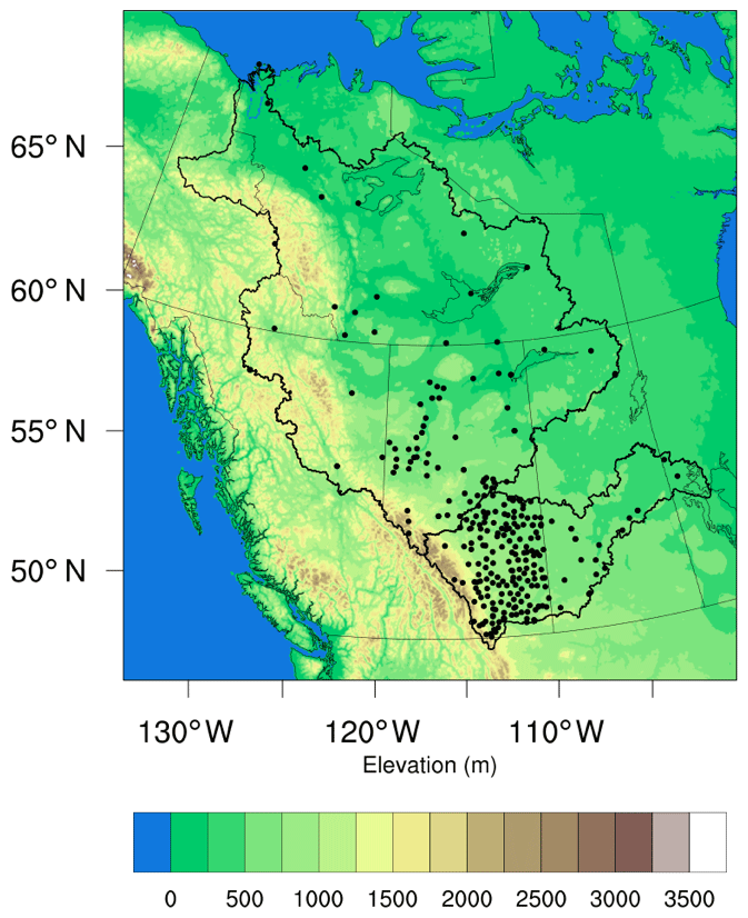
Figure 1The domain of WRF simulation. The black dots indicate the observation stations used in the evaluation of the simulations.
2.2 Numerical experiments
Two 15-year WRF simulations were conducted to simulate the regional climate under the historical and future climate using reanalysis and climate change forcing derived from CMIP5 ensembles, respectively. The control experiment (CTL), a retrospective/control simulation, aimed to reproduce the current climate statistics in terms of variability and mean state from 1 October 2000 to 30 September 2015. This control simulation was forced using 6-hourly 0.7∘ ERA-Interim reanalysis data (Dee et al., 2011) directly. WRF simulation was directly forced by 4 km one-way nesting without an intermediate buffering coarse grid between the ERA-Interim reanalysis and WRF domain because the ∼75 km resolution reanalysis was shown to be adequate (Liu et al., 2017). The second simulation was a climate perturbation or sensitivity experiment following the PGW approach used in Colorado Headwaters work (Rasmussen et al., 2011, 2014). Climate projections from GCMs introduce large uncertainties because of the substantial inter-model variability among GCMs (Deser et al., 2012; Mearns et al., 2013), which can obscure the climate change response due to global warming. Using the PGW approach with GCM ensembles can overcome the inter-model variability and isolate radiative forcing and its associated circulation as the sole reason for the regional climate response. Using PGW methodology during a future period also requires less computation resource than a continuous simulation spanning a century. However, the PGW method also has its disadvantages and limitations. Addition of climate change signal onto the reanalysis field may introduce an imbalance to the lateral boundary forcing because the nonlinear terms are not necessarily additive to balance the dynamics (Misra and Kanamitsu, 2004). PGW also does not fully consider the nonlinear interaction between global warming and atmospheric circulation changes, thus, cannot estimate the changes in future storm frequency, storm intensity, and the positions of storm tracks, which all interact with the large-scale climate system beyond the model boundary and could not represented by simply adding thermodynamic and kinetic change to current weather and climate (Sato et al., 2007).
Regional climate downscaling using convection-permitting models has a range of advantages over using models that rely on convection parameterization, including better convective precipitation simulation and the ability to compare regional climate changes directly related to global warming scenarios. Due to these benefits, convection-permitting PGW simulation (Liu et al., 2017) has been used in several recent studies to investigate the intensification of hourly precipitation extremes (Prein et al., 2017b), the decrease in overall precipitation frequency and light–moderate precipitation events over the contiguous US (CONUS) (Dai et al., 2017), the increase in rain-on-snow events in western North America (Musselman et al., 2018), and the change in cloud population (Rasmussen et al., 2017). The PGW forcing was derived from climate change signals from a 19-member ensemble mean of CMIP5 models. In particular, PGW 15-year (2000–2015) simulation was forced with the same period of 6 h ERA-Interim reanalysis as in CTL, plus a climate perturbation from the ensemble CMIP5 RCP8.5 projection:
where ΔCMIP5 RCP8.5 is the climate change signals derived from the CMIP5 multi-model (19 ensemble members) ensemble mean under the RCP8.5 emission scenario from 2071–2100 relative to 1976–2005. The choice of the model members and the details of the ensemble members of the 19 CMIP5 models are provided in Liu et al. (2017). Climate change signals are interpolated according to calendar date using the monthly ΔCMIP5 RCP8.5 data for both surface variables and three-dimensional field variables. The surface variables such as surface temperature, soil temperature, sea level pressure, and sea ice are incorporated into the PGW forcing by including the climate changes signals in the initial and boundary conditions for CTL. Similarly, PGW forcing perturbations were also added to the three-dimensional field variables, such as horizontal wind components, air temperature, specific humidity, and geopotential in the initial and boundary conditions of CTL.
The climate change signals in Fig. 2 show the circulation and thermodynamic changes in the PGW forcing for different seasons from the lower troposphere (750 hPa) to the jet-stream level (250 hPa). As shown in the third row of Fig. 2, the temperature increases at 750 hPa in the lower troposphere under RCP8.5. The warming is larger in the northwest and in the MRB than in the southwest and in the SRB, especially in autumn and winter. The warming ranges from 3 to 4 ∘C in winter and spring and from 4 to 5 ∘C in summer and autumn. Accompanying this warming is a moderate decrease (0.5 % to 2 %) in relative humidity throughout the domain, with a larger decrease in the south in summer and autumn. The change in geopotential height (GPH) at 750 hPa presents a pattern as thickness between the lower atmospheric isobaric surfaces, consistent with the temperature change, as the thickness is proportional to the average temperature of the layer. Accompanying this pattern of change in GPH, there is a weakening of the westerly flow in all seasons in the order of 0.5 to 1 ms−1 at 750 hPa due to geostrophic balance. At the mid-troposphere level, the general pattern of change in GPH at 500 hPa is similar to that at 750 hPa but with larger values of 90–100 m, as shown in the second row of Fig. 2. For the upper level at 250 hPa, the increase in temperature ranges from 1 to 4 ∘C, with stronger warming in the south, as shown in the top row of Fig. 2. The warming at 250 hPa is less than that at the lower levels, especially for the cold seasons, when the warming is only about 1 ∘C. The geopotential height experiences the largest increase in summer and the smallest increase in winter.
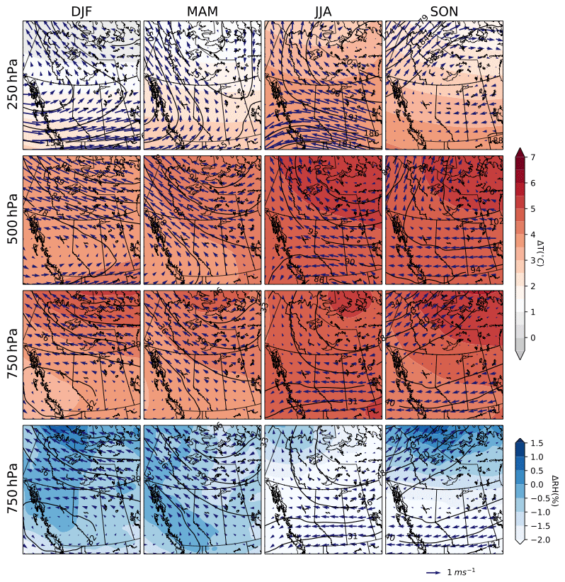
Figure 2The climate change signal in the PGW forcing-derived from 19-member CMIP5 ensemble for each season (from left to right: spring, summer, autumn, and winter) at the upper levels (250 hPa, first row; 500 hPa, second row) and lower atmosphere (bottom two rows). The contours are the changes in geopotential height relative to current climate. The shadings are changes in temperature or moisture at each pressure level. The wind vectors denote the change in the mean wind at each level.
2.3 Verification data
The simulation evaluation was conducted against two gridded datasets for temperature and precipitation for the retrospective CTL simulation from 2000 to 2015. The NCEP North American Regional Reanalysis (NARR) (Mesinger et al., 2006) and the surface station observations from Environment Climate Change Canada were also used in basin-averaged evaluations. Several facts have to be noted when conducting intercomparison between models, reanalyses, and gridded observations. The gridded observation dataset makes interpolations based on station observation, which makes ANUSPLIN less reliable in regions with complex terrain such as in the Canadian Rockies and areas with sparse observations like in the northern territories. Though NARR assimilates precipitation unlike most atmospheric reanalyses, the poor coverage of observation in Canada makes it also less reliable outside the populated regions in the southern Canada. As a result, NARR's performance is worse than CaPA and ANUSPLIN over western Canada, especially in cold seasons (Wong et al., 2017). Because CaPA incorporates both station observation and radar precipitation, it produces better spatial distribution of precipitation than ANUSPLIN (Fortin et al., 2018). Additionally, the different horizontal resolutions between models also introduce large differences in elevation in mountainous terrains, which can make the temperature and precipitation evaluation on a common grid difficult as the elevation difference can cause large temperature and precipitation biases. Finally, ANUSPLIN and CaPA still cannot capture mountain weather processes well. These gridded datasets are mainly based on ground observation and CaPA assimilates radar observation. The sparse observation network cannot adequately cover the area to delineate the drastic change in temperature and precipitation and the elevation placement of sites tend to be in the valley. Radar observation is also hindered by the topography. Winter precipitation observation often suffers from undercatchment due to boundary-layer processes. Therefore, the evaluation of WRF-CTL must be considered with these limitations in mind.
2.3.1 ANUSPLIN
ANUSPLIN was first used to develop a high spatial resolution (∼10 km) dataset of daily precipitation and minimum and maximum temperature for the period 1961–2003 for Canada (Hutchinson et al., 2009). ANUSPLIN uses a thin-plate smoothing spline algorithm composed of the spatially continuous functions of latitude, longitude, and elevation (Hutchinson et al., 2009). The algorithm offers an efficient way to develop spatially continuous climate distribution for temperature and precipitation (Xu and Hutchinson, 2013). Hopkinson et al. (2011) further improved the Canadian ANUSPLIN data through reducing significant residuals by aligning the climatological day at observation stations and expanding the gridded dataset to cover 1950–2011. The Canadian ANUSPLIN has been constantly updated and used to evaluate gridded climate models and reanalysis datasets (Eum et al., 2012) and to compare the impacts of different climate products on hydro-climatological applications (Bonsal et al., 2013; Eum et al., 2014; Wong et al., 2017). Our evaluation of CTL performance uses daily temperature, maximum temperature, minimum temperature, and precipitation from ANUSPLIN Canada.
2.3.2 CaPA
The Canadian Precipitation Analysis (CaPA) dataset is a precipitation reanalysis with high spatial resolution (∼15 km) and 6-hourly temporal resolution. CaPA is derived from various sources of precipitation data such as station observation, satellite remote sensing, weather radar, and short-term forecasts from the Global Environmental Multiscale (GEM) model (Mahfouf et al., 2007). The short-term precipitation forecasts from the Canadian Meteorological Centre (CMC) regional GEM model were used as the background field with the rain-gauge measurements from the National Climate Data Archive as the observations to generate an analysis error at every grid point (Mahfouf et al., 2007). CaPA's optimum interpolation method depends on three key parameters to specify the error statistics: background error, observation error, and characteristic length scale. The error statistics from observations and the background field were then used in the optimum interpolation technique to generate 6-hourly precipitation data. A recent paper by Fortin et al. (2018) presents a summary of the development and applications of CaPA in the last decade.
2.3.3 NARR
NARR uses the NCEP Eta Model together with the Regional Data Assimilation System to assimilate precipitation along with other variables. In NARR precipitation observations are assimilated using latent heating profiles (Mesinger et al., 2006) unlike most atmospheric analyses (e.g., ERA-Interim) that precipitation is prognostic instead of assimilated. NARR data are available from October 1978 to November 2018 at a relatively high spatial and temporal resolution: 32 km grid spacing, 45 vertical layers, and 3 h time intervals. The NARR dataset is used only for comparing basin-averaged temperature and precipitation for the SRB and MRB.
For the evaluation purpose, the coarser-resolution datasets are downscaled to WRF's 4 km grid. The coarser grid spacing in the interpolated observation and reanalyses means their surface elevation is smoother than that of the WRF simulation. Due to the difference in surface elevation as grid spacing changes, high-resolution WRF has higher peaks and lower valleys, which can introduce elevation-related temperature difference and orographic precipitation difference. The 4 km WRF simulation also provides more details for temperature and precipitation compared to coarse-resolution reanalysis and GCM outputs, especially over complex terrains in the Canadian Rockies. However, lack of high-resolution precipitation observations, such as those provided by NCEP Stage IV (Nelson et al., 2016) in the US, makes a thorough evaluation of the spatial features of 4 km WRF against coarse-resolution RCMs and GCMs over western Canada difficult. Here we show that 4 km WRF simulation produces much better mean precipitation distribution than GCMs in western Canada.
3.1 Near-surface temperature
Surface air temperature is a key meteorological variable that directly affects the daily life of human beings, physiological development of field crops, agricultural product quality, and various hydrological processes. For humans, extreme and persistent hot days in summer can cause health issues including heat cramps, heat exhaustion, and heat stroke, especially for vulnerable populations such as the elderly. For agriculture, extreme hot spells of multiple days with a maximum temperature hovering above the cardinal maximum, the temperature at which crop growth ceases, can significantly reduce crop yields. At the other extreme, the effects of very cold temperatures range from a minor inconvenience for some to severe infrastructure damage and increased mortality for vulnerable populations. As the mean temperature changes, the extreme distribution of temperature also changes substantially, sometimes more than the changes in the mean. From the perspective of hydrology, the surface air temperature's simulation is also crucial for obtaining realistic evapotranspiration, energy exchange between the surface and atmosphere, and phase transition of water near the ground. Because of all these temperature effects, evaluating the surface air temperature simulation is critical in laying the foundation for applying the WRF-CTL and PGW simulations to hydrological modeling, climate projection, and climate change impact analysis.
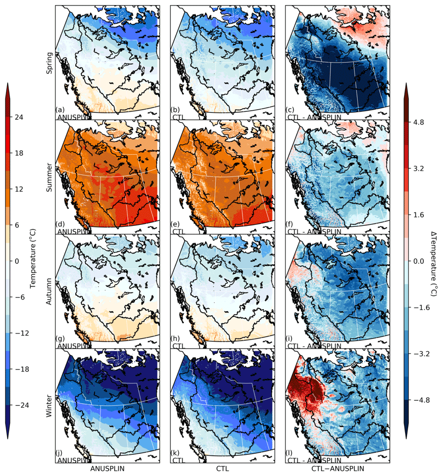
Figure 3Seasonal mean (from top to bottom: spring, summer, autumn, and winter) daily mean temperature for spring (MAM), summer (JJA), autumn (SON), and winter (DJF) from 2000 to 2015 of ANUSPLIN (left column), WRF-CTL (middle column), and the difference (CTL–ANUSPLIN, right column). The Δ sign indicates the bias of WRF-CTL relative to ANUSPLIN.
3.1.1 Mean temperature
The comparison of surface air temperature (2 m) between CTL and ANUSPLIN in Fig. 3 shows that WRF simulation of daily mean temperature agrees well with ANUSPLIN temperature in terms of the geographical distribution of cold biases east of the Canadian Rockies, especially in spring. The spring (March, April, May), summer (June, July, August), autumn (September, October, November) and winter (December, January, February) from WRF-CTL and the gridded observation analysis ANUSPLIN are presented in Fig. 3. Both ANUSPLIN and CTL show a consistent spatial distribution and seasonal change in temperature gradient. In spring there is a strong cold bias (about −5 ∘C) over the Canadian Prairies, with a small warm bias of 1–2 ∘C in the northeastern domain. In summer the hottest region is located in the southern Canadian Prairies, with temperatures decreasing toward the northeastern and coastal regions. In autumn the temperature in both ANUSPLIN and WRF decreases from the southern border to the Arctic. However, there are a few noticeable biases in the simulated daily mean temperature. In winter and spring, the temperature decreases from southwestern British Columbia toward the northeast of the domain as the regional climate changes from oceanic to subarctic. There is a significant warm bias (about 3–4 ∘C) in winter near the Yukon and western Northwest Territories, which is likely inherited from the forcing since it is also present in ERA-Interim but with smaller magnitude (2 ∘C) as seen in Fig. S3. In winter small warm biases (about 2 ∘C) also occur in central and northern British Columbia. To the east there are small cold biases (−1 to −2 ∘C) in all seasons east of the Canadian Rockies, where the forcing data ERA-Interim have small warm biases (about 1 ∘C) compared to ANUSPLIN in the region. Due to these biases in winter and spring, the WRF-CTL simulation tend to enhance the temperature difference between the warmer regions near the Pacific coast and the colder Canadian Prairies. Although regional climate models are forced by reanalysis data on the boundary and underlying surface, the near-surface temperature is strongly affected by the representation of surface processes and boundary-layer energy exchange. The cold bias in spring over the Canadian Prairies is caused by several factors: wet biases in precipitation and cold biases in temperature in winter and the overestimation of snow cover in the region, which amplifies the cold bias in spring through snow-albedo feedback. WRF-CTL shows a slight warm bias in the valleys of southern British Columbia, where WRF's high-resolution grid has lower elevations than the ANUSPLIN grid and where ERA-Interim shows a cold bias due to its coarser resolution and inability to resolve the valleys.
3.1.2 Daily minimum and maximum temperature
The daily minimum temperature (Tmin) of WRF-CTL and ANUSPLIN (Fig. S1 in the Supplement) shows a similar geographical distribution to that of the daily mean temperature in all seasons. The main difference between the Tmin distribution and daily mean temperature distribution is that the south–north temperature gradient becomes less in summer. Compared to the bias of daily mean temperature, WRF-CTL simulation of Tmin relative to ANUSPLIN shows a stronger warm bias in the northwest (the Yukon and western Northwest Territories), with a magnitude of 4 ∘C in winter. Additionally, the cold bias of CTL in Tmin over the Prairies in spring decreases by 50 % compared to that of the daily mean temperature (about −2 to −4 ∘C vs. −6 ∘C).
The daily maximum temperature for four seasons by WRF and ANUSPLIN is shown in Fig. 2. The cold bias in the Prairies during spring shown in the Tmax is more pronounced (>6 ∘C) than in the daily mean temperature. The warm bias in the northeast in spring is also stronger. The Tmax and Tmin bias distribution shows that the cold bias in spring in the Prairies is stronger in the early afternoon, when there is strong solar insolation, and much weaker at night. This cold bias in spring may relate to a combination of the overestimation of snow cover and the albedo biases associated with improper representation of snow in the land surface model (Meng et al., 2018).
3.2 Precipitation
Water resources are of strategic significance for the environment, agriculture, and society, especially for semi-arid regions in most of western Canada. Precipitation is an important component of water balance and is essential for hydrological modeling as all runoff comes from precipitation, either directly or indirectly. The ability of climate models to capture the temporal–spatial characteristics of observed precipitation is crucial for their application as input for hydrological models. GCMs' precipitation simulations are known to be one of the most challenging tasks for climate modelers as precipitation processes involve many subgrid-scale processes that have to be parameterized. Also, due to resolution limits, GCM's precipitation output has to be downscaled to be applicable in regional- and local-scale hydrological and ecological studies. The purpose of the WRF simulations is to dynamically downscale the current climate using ERA-Interim reanalysis and a future RCP8.5 climate projection based on the ensemble mean of 19 CMIP5 models. Especially, using a convection-permitting resolution, the WRF model avoids the utilization of convection parameterization, which introduces large biases and distortion in simulating convective precipitation systems. Figure S6 shows the CMIP5 GCM ensemble mean precipitation that differs from the observed pattern of seasonal precipitation distribution: the high-precipitation band near the British Columbia coast is much broader; the dry area between mountain ranges and a secondary peak on the eastern edge of the Canadian Rockies are missing. Both features are well captured by WRF-CTL. Due to the poor performance of GCM precipitation simulation and coarse-resolution reanalysis, we did not conduct a full evaluation of the WRF-CTL precipitation against any GCM output or reanalysis with coarse resolution (>25 km).
The number of global gridded precipitation datasets has grown in recent years with increasing coverage of satellites; however, the quality of the precipitation analysis is still limited by the number of observation stations over Canada, especially in the complex terrain in the Canadian Rockies and the northern territories, where only a few observation sites scatter across a vast domain. Wong et al. (2017) compared multiple precipitation products over Canada for various climatic zones and river basins against station observation and found the performances of CaPA and ANUSPLIN are generally superior to other datasets, even though both datasets perform poorly in the mountainous regions and northern territories. Furthermore, ANUSPLIN's coverage over the northern part of western Canada relies on a very limited number of stations and shows a large dry bias in the regions. CaPA, a reanalysis dataset, has been shown to have better overall spatial distribution of precipitation than ANUSPLIN (Fortin et al., 2018; Wong et al., 2017). Bearing these in mind, we conducted the evaluation of precipitation against two observation precipitation analysis datasets, ANUSPLIN and CaPA.
As shown in Figs. 4 and S4, the WRF-CTL simulation captures the main precipitation distribution pattern in the observed precipitation from CaPA and ANUSPLIN, respectively: high precipitation near the British Columbia coast in winter and over the immediate region on the lee side of the Canadian Rockies in summer. WRF-CTL's spatial pattern more closely resembles CaPA's and bears noticeable difference to ANUSPLIN's, especially over the eastern ranges of the Canadian Rockies. Both CaPA and WRF-CTL are significantly wetter than ANUSPLIN, especially in the mountainous region and northern part. Compared to ANUSPLIN in Fig. S4, WRF-CTL's wet bias mainly resides over the mountain ranges by the Pacific Ocean and in the Canadian Rockies. This wet bias associated with topography is as high as 1.7 mm d−1 and more prominent in winter and spring. It must be considered, though, that gridded observation analyses often underestimate precipitation over mountains, where data are scarce, through interpolation from available lower-elevation observations. East of the Canadian Rockies, there are moderate wet biases (about 0.5–0.9 mm d−1) across the Prairies and the boreal forest. In terms of WRF-CTL's relative bias in reference to ANUSPLIN, there is significant wet bias (+90 %) in the northern domain, including the MRB for all seasons. For the SRB, a large dry relative bias occurs in winter due to low observed precipitation during this season. However, according to the evaluation by Wong et al. (2017), ANUSPLIN underestimates annual precipitation by 10 % to 50 % from the south to north of western Canada relative to gauge observation in the region from 2002 to 2012. Thus, the large wet bias of WRF-CTL relative to ANUSPLIN in the north is largely due to the large dry biases of ANUSPLIN there.
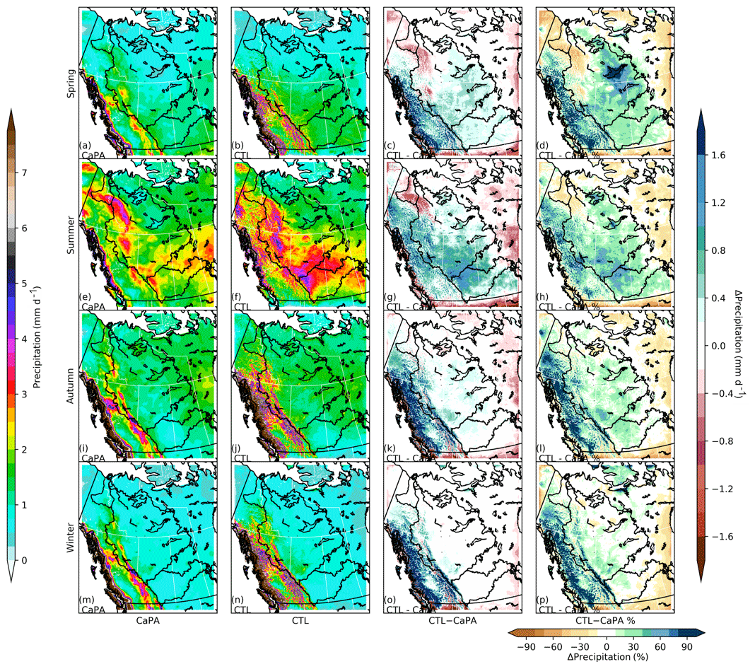
Figure 4Seasonal mean (from top to bottom: spring, summer, autumn, and winter) daily precipitation from CaPA (first column) and WRF-CTL (second column), and their absolute (third column) and relative differences in percentage (fourth column). The Δ sign indicates the bias of WRF-CTL relative to CaPA.
Relative to CaPA, the wet bias of WRF-CTL is generally less in magnitude and less correlated with topography because CaPA assimilates GEM forecast and remote sensing data to better represent orographic precipitation than analysis data, which rely heavily on rain gauges located at lower elevations. The wet bias along the British Columbia coastal mountain ranges and the Canadian Rockies are prominent in spring, autumn, and winter. East of the Canadian Rockies, the wet bias is located mainly over the SRB and southern MRB in spring and summer. There are also regions of dry biases in the region surrounding the MRB and SRB in spring, summer, and autumn. In winter the difference between CTL and CaPA is small east of the Canadian Rockies. It is noteworthy that, according to Wong et al. (2017), the WRF-CTL wet bias relative to CaPA's east of the Canadian Rockies may be partly attributed to CaPA's relatively small dry bias (10 %) relative to station observation.
In summary, the WRF-CTL simulation captures well the spatial distribution of precipitation in all seasons. WRF-CTL's agreement with CaPA is more widespread and consistent. There are wet biases in WRF-CTL over the mountainous region compared to both ANUSPLIN and CaPA. According to the evaluation of Wong et al. (2017), both ANUSPLIN and CaPA show wet bias in the mountainous region compared to station observation, but this may be because the stations are usually situated at low altitudes and thus fail to capture the representative areal precipitation due to the topography. East of the Canadian Rockies, WRF-CTL shows a wet bias relative to ANUSPLIN and CaPA, although both the observation and reanalysis datasets show dry bias from 2002 to 2012 in the region, especially in the northern part.
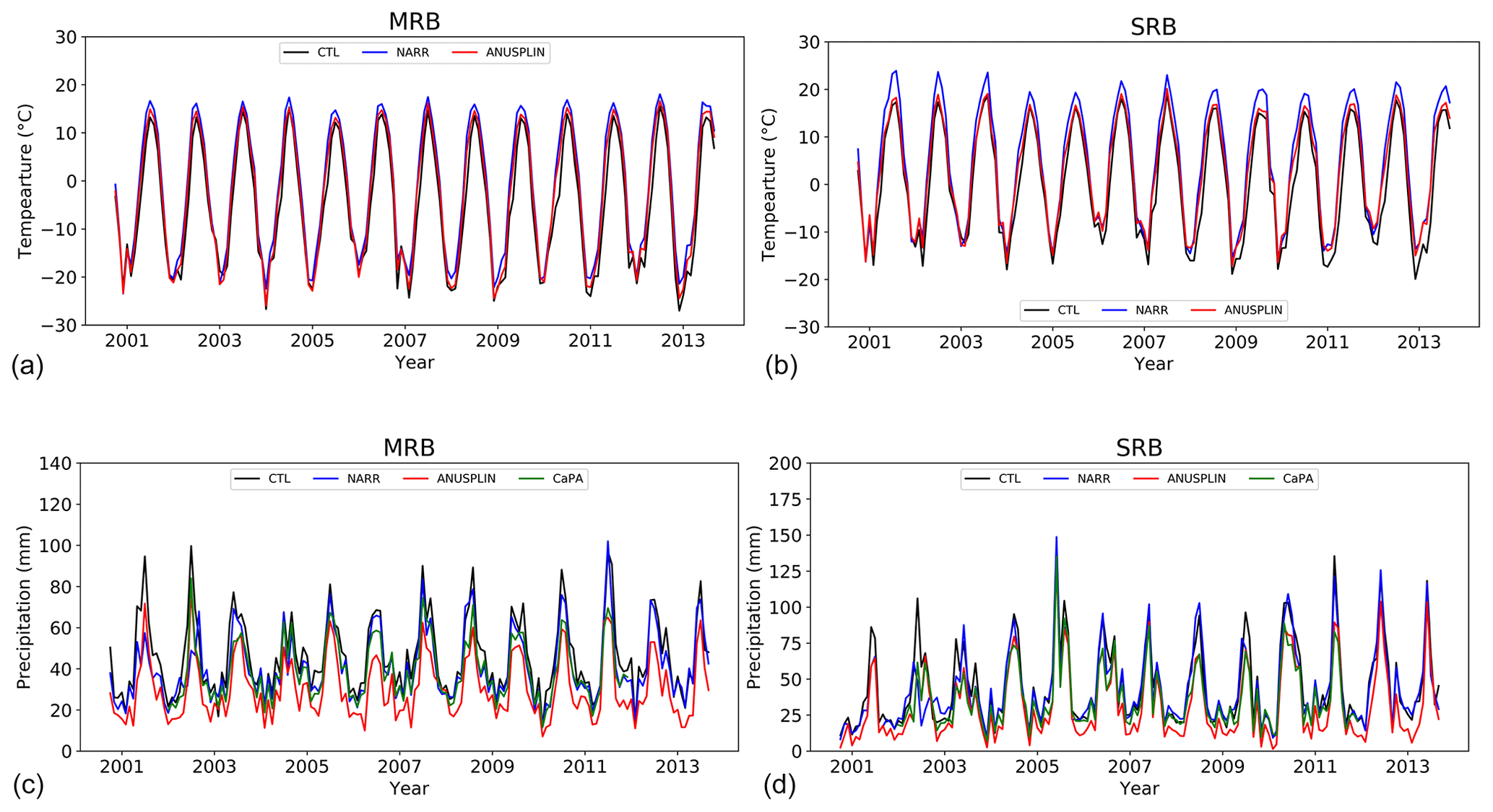
Figure 5The monthly mean precipitation/temperature averaged over the Mackenzie River basin (a, c) and Saskatchewan River basin (b, d) from 2000 to 2015 from WRF-CTL (black curve) and an ensemble of observation/reanalyses of temperature (NARR, blue; ANUSPLIN, red) and precipitation (NARR, blue; ANUSPLIN, red; CaPA, green).
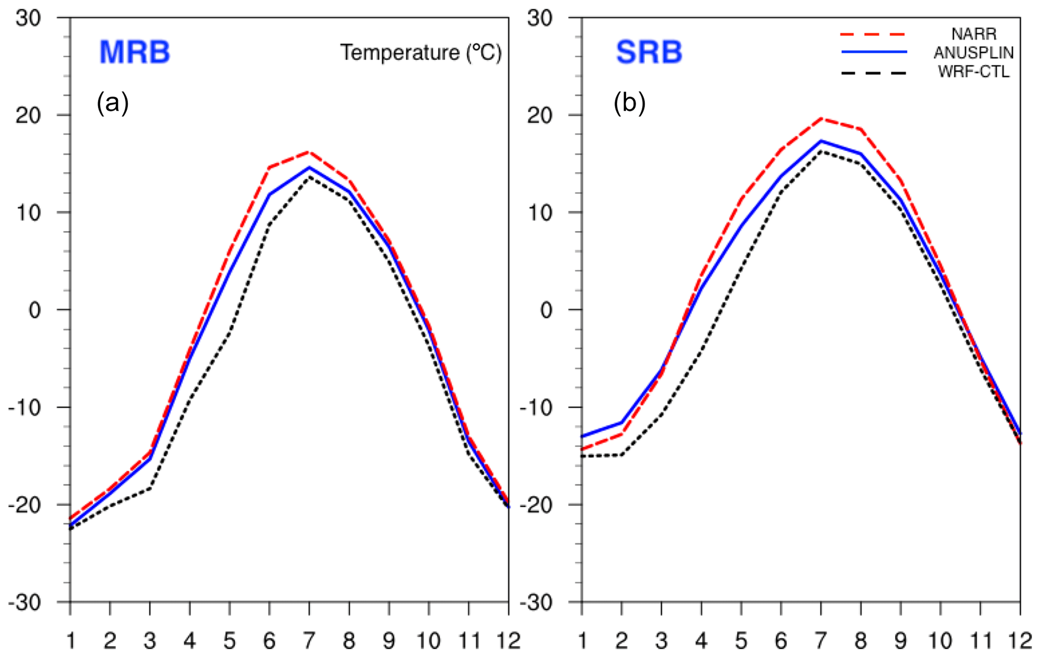
Figure 6The mean annual cycle for WRF-CTL (black), NARR (red), and ANUSPLIN (blue) over the Mackenzie River basin (a) and Saskatchewan River basin (b). Monthly basin-averaged precipitation over the Saskatchewan River basin from WRF-CTL, the WRF-CONUS control run, and the ensemble of observation datasets (NARR, ANUSPLIN, CaPA).
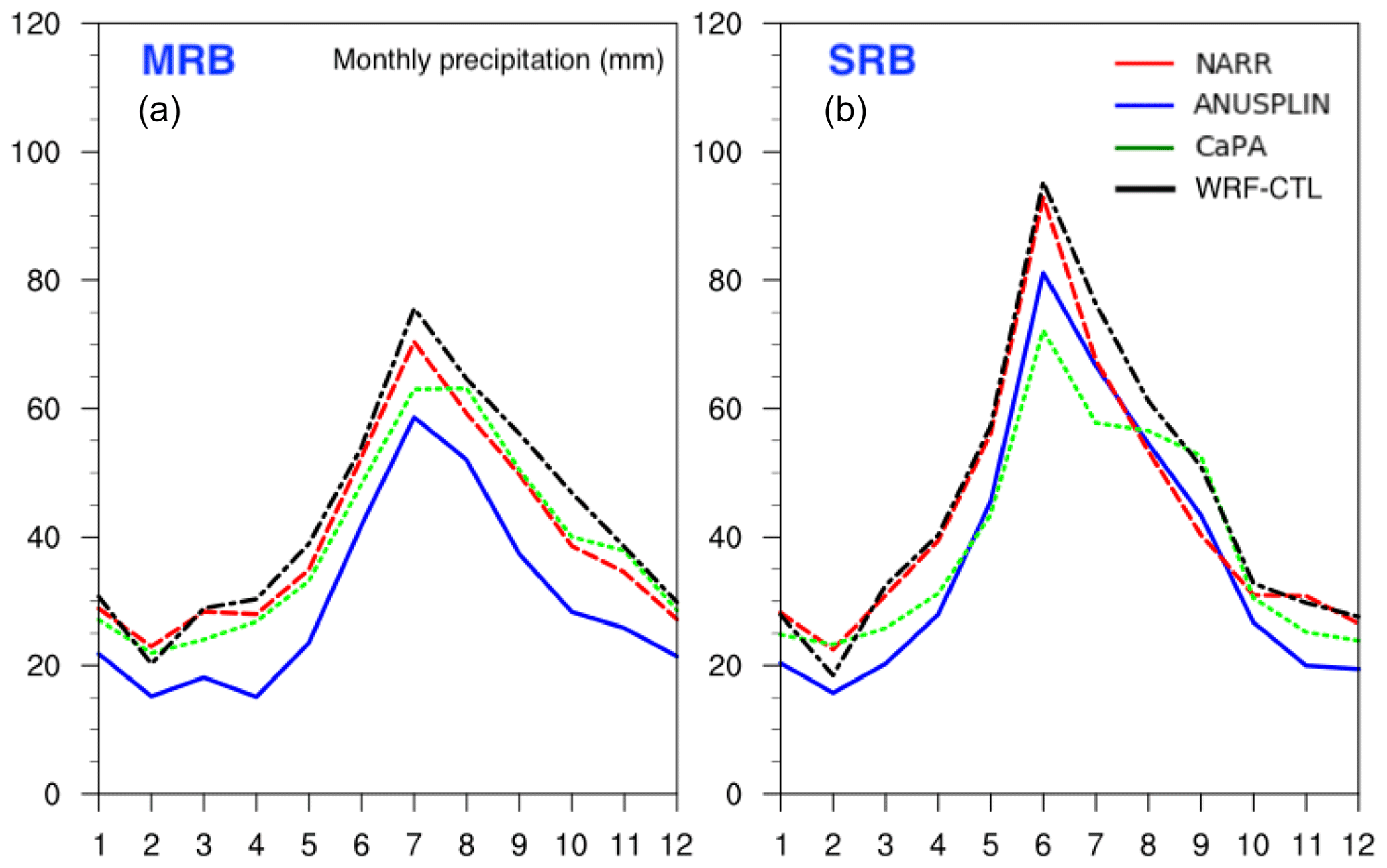
Figure 7The mean annual cycle of monthly precipitation for WRF-CTL (black), NARR (red), and ANUSPLIN (blue) over the Mackenzie River basin (a) and Saskatchewan River basin (b).
3.3 Basin-averaged statistics
The evaluation of the simulation over the two major river basins focuses on the model performance in simulating the seasonal and interannual variations of the two key variables for hydrology: temperature and precipitation. To validate the WRF simulation results in the MRB and SRB, we compared them with several existing observation and reanalysis products. Figure 5 shows the time series of basin-averaged temperature (top) and precipitation (bottom) in the MRB (left) and SRB (right) for the simulation period, together with different observation and reanalysis datasets (NARR, ANUSPLIN, CaPA). Figure 6 shows the mean annual temperature cycle from WRF-CTL (black), NARR (red), and ANUSPLIN (blue) for the MRB. Figure 7 shows the annual cycle of precipitation for the two basins.
3.3.1 Mackenzie River basin
The WRF simulation faithfully reproduces the seasonal and interannual variations of temperature of the MRB. Compared to the observation, the WRF temperature simulation is within the observation spread but on the lower end of the distribution in the MRB. NARR is generally much warmer than both ANUSPLIN and WRF-CTL during summer. The WRF simulation shows a cold bias for the whole year, especially from March to July compared to ANUSPLIN. The simulated basin-averaged precipitation matches well with the observation in terms of interannual variability and seasonal cycle. This good match indicates confidence in the ability of WRF-CTL to capture the main characteristics of precipitation regime changes year on year, despite biases in the total amount. ANUSPLIN shows much lower basin-averaged precipitation in the MRB throughout the year, which is consistent with previous evaluations (Wong et al., 2017). The simulated precipitation shows a wet bias as the WRF-CTL curve is almost always on the top of the observation envelope, especially for spring and summer. As shown on the left in Fig. 7, the mean annual cycle of precipitation over the MRB is compared between WRF-CTL, the reanalysis CaPA, NARR, and observation analysis, ANUSPLIN. Both WRF and CTL simulated and observed a precipitation peak in July. The simulated precipitation by WRF-CTL is higher than ANUSPLIN in all months and very close to NARR and CaPA, except in summer when it is about 5 mm per month wetter than NARR and CaPA on average.
3.3.2 Saskatchewan River basin
The WRF simulation captures the seasonal and interannual variation of temperature in the SRB. Compared to the observation, the WRF simulation is close to ANUSPLIN with a cold bias in spring and slight cold biases in other seasons. NARR is much warmer than WRF-CTL and ANUSPLIN in the warm season, with a basin-averaged bias as large as 5 ∘C. According to Fig. 6, the annual cycles of temperature from WRF, NARR, and ANUSPLIN show good agreement for the SRB. The WRF simulation shows a cold bias for the whole year relative to ANUSPLIN, especially from March to July. The cold bias for the SRB is larger than that of the MRB, which is consistent with the spatial distribution of temperature bias in Fig. 3, where cold biases in the Prairies are stronger in spring over the Saskatchewan River basin.
Figure 5 shows the simulated monthly precipitation by WRF-CTL over the SRB (solid black line) from 2001 to 2013 among gridded analysis and reanalyses for most of the years. WRF-CTL precipitation is comparable to the precipitation from NARR, ANUSPLIN, and CaPA in the SRB in general. WRF-CTL is significantly wetter than other datasets during summer of 2002–2003 when the Prairies experience drought. The simulated basin-averaged precipitation shows a similar seasonal cycle and interannual variability and as observation, as shown in Fig. 7. The simulated and analysis/reanalyses precipitation data peak in June with the amount of about 60 to 90 mm, and also show the least amount of monthly precipitation in winter, with about 20–30 mm. Again, the precipitation simulated by WRF-CTL is closer to NARR and CaPA than it is to ANUSPLIN over the SRB. ANUSPLIN is much drier than other datasets especially in cold seasons. The simulated precipitation has a wet bias for all seasons compared to CaPA and ANUSPLIN, with the WRF-CTL-simulated curve almost always at the top of the observation envelope, as shown in Fig. 7.
Regional climate modeling as a dynamical downscaling tool generates not only climate projections with a higher spatial resolution, but also hydroclimatic regimes different from GCMs and statistical downscaling. These improvements can be attributed to enhanced representation of fine-scale processes in the atmosphere and boundary conditions.
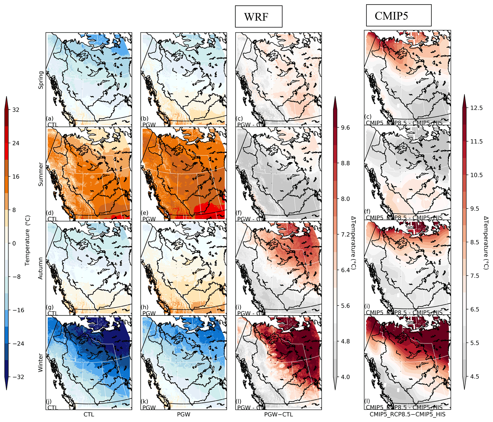
Figure 8Daily mean temperature from WRF-CTL (first column) and WRF-PGW (second column), the difference (PGW–CTL, third column), and the projected warming from the CMIP5 ensemble (2071–2100 to 1976–2005, fourth column) for spring (first row), summer (second row), autumn (third row), and winter (fourth row).
4.1 Near-surface temperature
The daily mean temperature simulated by WRF-CTL and WRF-PGW, and the warming in WRF-PGW relative to CTL are presented in Fig. 8 together with the projected warming by CMIP5 ensemble (2071–2100 to 1976–2005). The temperature increase in WRF-PGW is larger in the northeastern domain and smaller in the southwest, generally reducing the northeast–southwest temperature gradient in CTL climatology in all seasons. The warming is the greatest in winter, with a 10 ∘C increase in the northeastern quadrant. In the Prairie, the largest warming occurs in the spring. This larger warming over the Prairies is related to the shift of the daily mean temperature from below freezing in early and mid-spring to above freezing, likely causing amplified warming through snow-albedo feedback. The mean temperature in the Yukon and NWT will be similar to those currently experienced in Saskatchewan and Alberta in spring and summer, which has great implications for the length of the growing season in the northern territories. The winter temperature in the coldest region of the domain will be as warm as the central Canadian Prairies in the current climate. The higher temperatures in the boreal forest region will greatly increase the probability of wildfire, water stress, and insect pests, threatening the boreal forest ecosystem, which could eventually be replaced by grassland and parkland (Stralberg et al., 2018). As shown in Figs. 8 and S5, CMIP5 ensemble projection indicates a larger warming for all seasons than WRF projection and different spatial pattern for spring and summer. In spring WRF has larger warming (about 7 ∘C) in the Canadian Prairies and about 6 ∘C warming in the north comparing to CMIP5 has a warming of 9 ∘C in the north and about 5 ∘C in the Canadian Prairies. In summer, WRF shows a 5 ∘C warming in most of the domain except for the northeastern corner (about 6 ∘C warmer); CMIP5 shows a much stronger warming in the southern domain, about 7 ∘C, south of 55∘ N. The stronger summer warming in CMIP5 over the southern domain is consistent with the decrease in summer precipitation in the region.
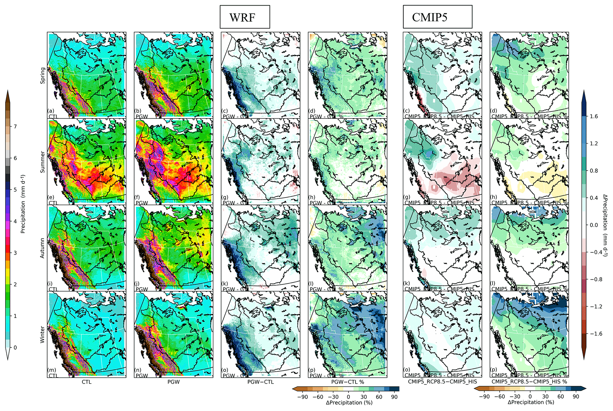
Figure 9From top to the bottom, spring, summer, autumn, and winter seasonal mean daily precipitation are shown for WRF-CTL (first column), WRF-PGW (second column), the difference (PGW–CTL, third column), and percentage difference over CTL (fourth column). On the right-hand side, the projected changes from the CMIP5 ensemble for precipitation (2071–2100 to 1976–2005, fifth column) and in percentage (sixth column) are shown.
4.2 Precipitation
The comparison of WRF-PGW and WRF-CTL precipitation is shown in Fig. 9. Generally speaking, the precipitation will increase in most of the domain. In most places, WRF-PGW shows an increase in precipitation of about 15 %–30 % in all seasons compared with WRF-CTL. Near the British Columbia coast, the magnitude of the increase can be as large as 2 mm d−1. This substantial increase in precipitation in British Columbia's coastal mountains is related to the larger water vapor loading in PGW and the stronger effective orographic lifting to produce precipitation in that region. The change in precipitation is the least in summer, when parts of the Prairies receive less precipitation in PGW than in CTL. With almost no increase in summer precipitation and the much larger evapotranspiration in the Canadian Prairies in PGW than in CTL, the water availability during the growing season will be challenging for the Canadian Prairies. The dynamic downscaling by WRF is less pessimistic for growing season water availability in the Canadian Prairies than CMIP5 ensemble projection in Figs. 9 and S6, which shows a much larger decrease (−10 %–20 %) in precipitation in summer in the southern part of the domain including the SRB and southern MRB. In the northeastern portion of the domain, northern Manitoba and NWT, the precipitation increase could be as large as 0.5–1 mm d−1, with an increase of about 40 % in autumn and winter. The Yukon and central–northern British Columbia are expected to have a 40 % increase in precipitation in winter due to the higher loading of water vapor in a warmer climate. In addition to wetter projection for the Canadian Prairies in summer, the WRF projection also shows a larger increase in precipitation near the British Columbia coast, along the eastern mountain ranges of the Canadian Rockies throughout the year in Fig. 9. These regions have significant orographic lifting, which is better represented in WRF than GCMs, to initiate convection and/or precipitation and convert the higher water vapor concentration in a warmer climate to higher precipitation. GCMs' poor representation of orography may be the reason that less precipitation increases are generated over these terrains.
4.3 Basin-averaged changes compared to CMIP5
Here we compare the regional-averaged temperature and precipitation for two major river basins and for output from CMIP5 vs. 4 km WRF. Figures 10 and 11 show the temperature and precipitation changes between 1976–2005 and 2071–2100 as projected by CMIP5 ensembles and those of WRF-CTL (2000–2015) and PGW with 2070–2100 climate forcing simulation.
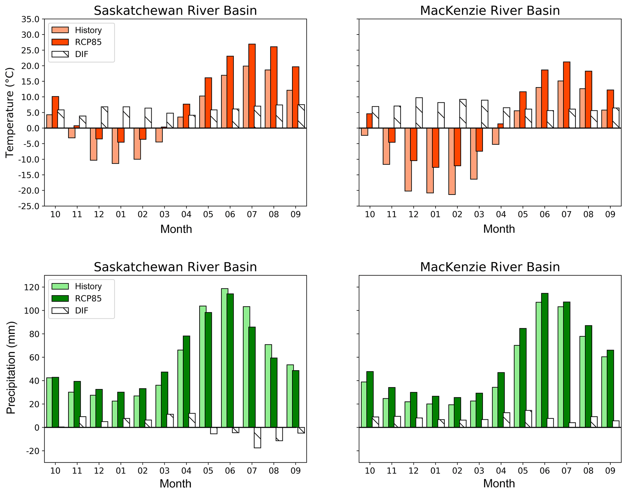
Figure 10Annual cycle of temperature and precipitation projected by CMIP5 ensemble. The orange bars indicate the basin-averaged temperature of the current climate (1976–2005). The red bars represent the basin-averaged temperature at the end of the 21st century under RCP8.5 (2076–2100). The white bars denote the change in temperature at the end of the century relative to the current climate. The dark green bars indicate the basin-averaged precipitation of the current climate. The shallow green bars represent the basin-averaged precipitation at the end of the 21st century under RCP8.5. The white bars denote the change in precipitation.
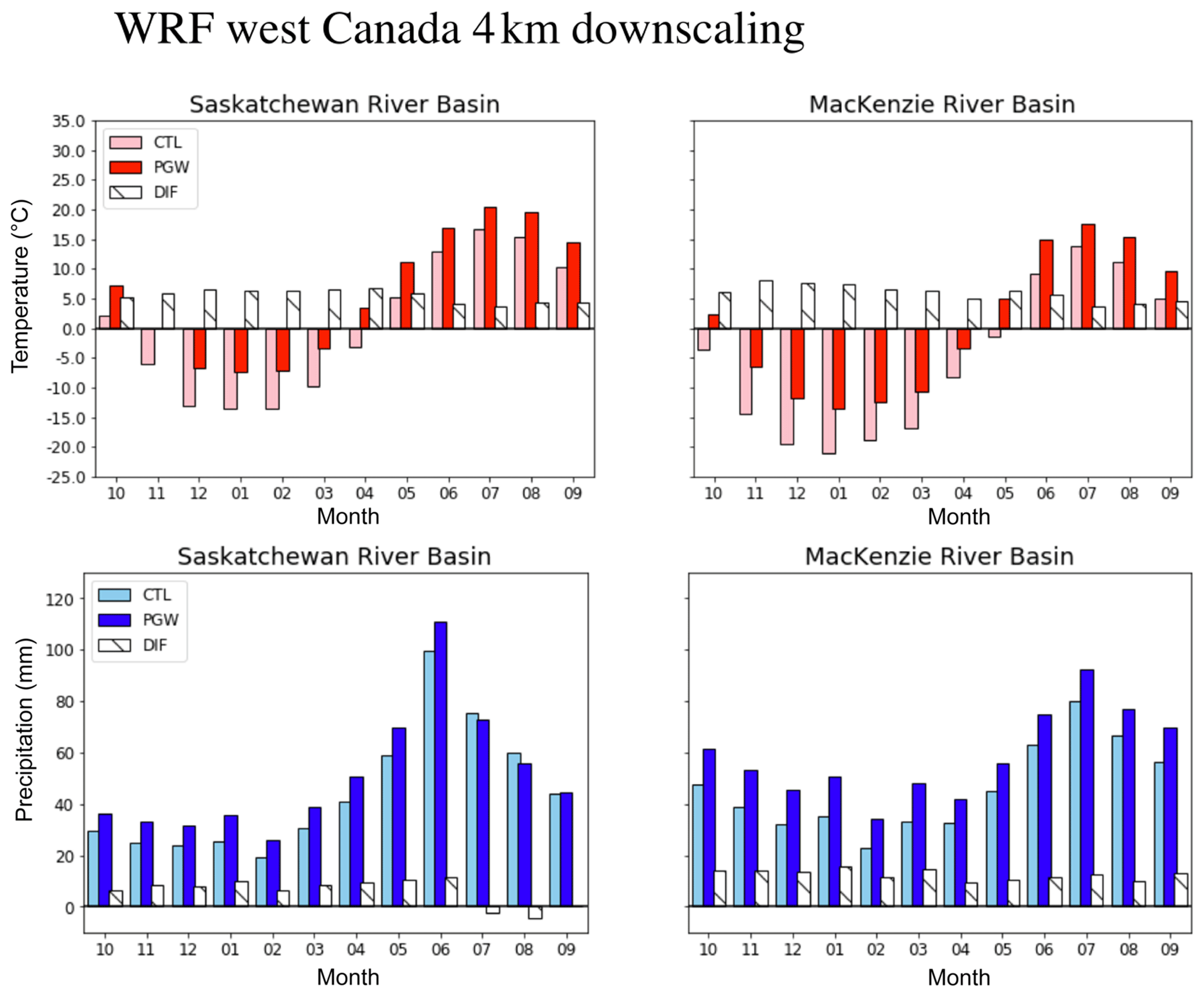
Figure 11Annual cycle of temperature and precipitation projected by WRF-PGW (2001–2015). The pink bars indicate the basin-averaged temperature of current climate. The red bars represent the basin-averaged temperature at the end of the 21st century under RCP8.5. The white bars denote the change in temperature at the end of the century relative to the current climate. The dark blue bars indicate the basin-averaged precipitation of the current climate. The shallow blue bars represent the basin-averaged precipitation at the end of the 21st century under RCP8.5. The white bars denote the change in precipitation.
In Figs. 10 and 11, the historical runs are shown in the red/orange columns for temperature for CMIP5/WRF-CTL; the future runs equivalent to the end of the 21st century are shown in the light red/orange columns for the temperature of CMIP5-RCP8.5/WRF-PGW, and the difference between the future simulation and the historical simulation are represented by the white columns. In general, temperature will increase for all months for both CMIP5 and WRF in both basins. The temperature increases in most months for the SRB are smaller in the WRF simulation than they are in CMIP5, especially in summer. The temperature increases in the MRB are about 3 ∘C smaller in WRF in December and February and about 2 ∘C smaller in summer. For the MRB, the temperature increase simulated by WRF is smaller than the CMIP5 ensemble mean for most months.
The historical precipitations are shown in the dark blue/green columns in Figs. 10 and 11; the future precipitations equivalent to the end of the 21st century are shown in the light blue/green columns, and the differences between the future run and the historical run are represented by the white columns. The projected changes from the CMIP5 ensemble and WRF show seasonally dependent differences. In the MRB, the precipitation increase in WRF-PGW simulation is lower in April and May and higher in other months compared to that in CMIP5. For the SRB the ensemble of the CMIP5 RCP8.5 projection shows that the winter and early spring precipitation will experience a large increase and the warm season (May–September) precipitation will decrease, especially in July. In contrast to this, WRF shows a large increase in precipitation in June and smaller decreases in precipitation in July and August, with moderate increases in other months in the SRB. Due to this difference in the annual cycle of precipitation change in the SRB, the dynamical downscaling by WRF-PGW shows an increase in precipitation before July, whereas the CMIP5 ensemble projection increases the precipitation before May.
Precipitation in summer and late autumn for the SRB either remains unchanged or shows a decrease for both the WRF-CTL and CMIP5 ensembles. This seasonal difference in precipitation change indicates that the Canadian Prairies and the southern boreal forest biomes will likely see a slight decline in precipitation minus evapotranspiration during the summer months, possibly affecting soil moisture for farming and forest fires. Because the precipitation increases substantially in spring in both the SRB and MRB, when combined with large temperature increases in spring, western Canada may experience more frequent rain-on-snow events that can cause severe flooding. This projection calls for thorough investigations that combine the high-resolution regional climate simulation and state-of-the-art hydrological modeling to quantify the probability of catastrophic flooding in spring over western Canada (Li et al., 2017).
4.4 Daily precipitation frequency distribution
For both hydrological applications and societal impacts, the temporal precipitation distribution and precipitation intensity distribution are as important as the total amount of precipitation. For example, more high-intensity precipitation events tend to cause flash flooding and sharp spikes of runoff, while lower effective precipitation during warm seasons increases the possibility of drought and fire.
The probability density function (PDF) of precipitation shows the distribution of precipitation amounts among both light and intense precipitation events. Figure 12 shows the probability density function of daily precipitation for the simulation of WRL-CTL and WRF-PGW and observation from CaPA and ANUSPLIN in the MRB (top two rows) and SRB (bottom two rows). In the top panel, the precipitation intensity is shown with a linear scale on the x axis and a logarithmic scale on the y axis for a probability density function (PDF) to show the detail in high-end precipitation. Compared to that of ANUSPLIN and CaPA, the WRF-CTL-simulated precipitation shows a heavy tail on the high end of the distribution, indicating that the bias in WRF-CTL mean precipitation relative to ANUSPLIN and CaPA in the MRB is largely caused by a larger number of heavy precipitation events. WRF-PGW future simulation shows an even higher distribution for extreme precipitation events, indicating that these events will become even more severe under future climate conditions. In the lower panel, both log −X and log −Y are used for precipitation and probability density, enabling us to zoom in on the probability distribution of the light-to-moderate events. The red curve, the WRF-PGW future climate simulation, is now underneath CTL, ANUSPLIN, and CaPA curves in events lower than 5 mm d−1, especially in summer (JJA). This means that the MRB is expected to experience fewer moderate precipitation events in addition to an increase in the probability of high-intensity precipitation.
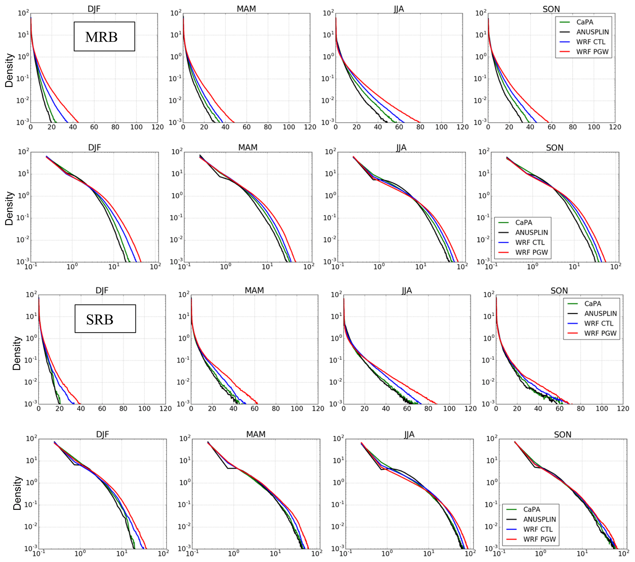
Figure 12Daily precipitation probability density function in the Mackenzie River basin (top two rows) and Saskatchewan River basin (bottom two rows) for WRF (CTL, PGW) and CaPA and ANUSPLIN with linear–log and log–log axes for density (y) and amount (x).
For the SRB, the bottom two rows of Fig. 12, the difference between WRF-CTL (blue curve), ANUSPLIN, and CaPA is less than that in the MRB. This difference is consistent with the spatial distribution of precipitation bias in Figs. 4 and S4, where the bias in the SRB is much smaller than it is in the MRB. WRF-PGW shows that heavy precipitation events increase and that their distribution trends towards more extreme intensive events in all seasons, especially in summer. Similarly to the MRB, there is also a decrease in moderate precipitation events, shown in the log −log plot in the second row. Due to this shift in precipitation intensity to the higher end in the PGW simulation, the seemingly moderate increase in total amounts in summer for both basins may not reflect the real change in flooding risk and water availability for agriculture. Although the total amount of precipitation is expected to increase in the future, there will be less water for agriculture because extreme precipitation will contribute more to runoff than soil moisture, reducing its accessibility to crops.
As seen in Fig. 12, the intervals between light to moderate precipitation events increase, because the total summer precipitation slightly increases and heavy precipitation events significantly increase, while the atmosphere needs more time to replenish water vapor (Dai et al., 2017; Trenberth et al., 2003). Dry spells also increase in frequency because both evaporation and the intervals between precipitation events increase. The intensification of droughts will have a wide-reaching impact beyond the agricultural sector: conditions are likely to be ideal for wildfires, like those experienced across the western provinces and territories from 2014 to 2018.
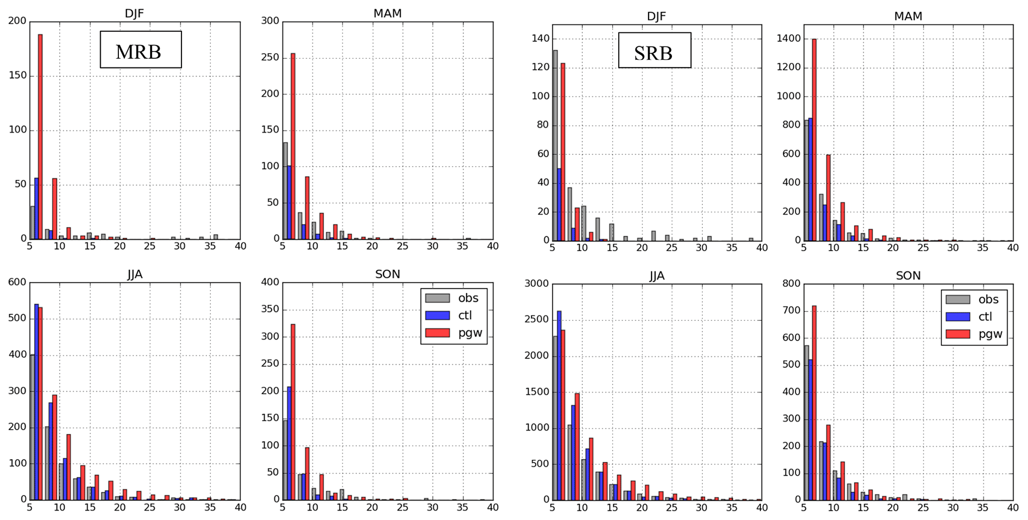
Figure 13Three hourly precipitation distribution from station observation in the MRB (left) and SRB (right) and those corresponding to WRF-CTL and WRF-PGW simulations.
4.5 Hourly precipitation extremes
The future distribution of subdaily precipitation extremes in western Canada is of particular concern, as they can cause flash floods and landslides, which damage human infrastructure and result in injuries and deaths. Here we compare the 3-hourly precipitation rate distribution among station observation, WRF-CTL, and WRF-PGW in the two basins and then investigate the changes in the hourly precipitation rate distribution. The 3-hourly precipitation rate is first compared to observation to evaluate the extreme precipitation simulation at 3 h intervals. The 3-hourly precipitation histograms for extreme precipitation events in the MRB and SRB are shown in Fig. 13. WRF simulations are compared with EC station observations in Fig. 1 because these station observations are closer to the ground truth than the gridded observational products for which the spatial resolution is 10 km at most and are shown to have biases (Wong et al., 2017). Only the moderate to extreme values of precipitation distribution are shown here by cutting it off at a precipitation rate of 5 mm/3 h. WRF-CTL's precipitation distribution (the blue columns) is close to that of the station observation (the gray columns) in the SRB in spring, summer, and autumn, whereas WRF-CTL produces more light to moderate precipitation events than observation in the MRB in most seasons except spring. These results indicate that the WRF simulation captures the local precipitation extremes in all seasons well, except winter in the SRB. WRF also shows a wet bias in light to moderate rain events in the MRB in all seasons but spring, while WRF-PGW simulations (the red columns) show a significant increase in the frequency of high-intensity rainfall events across seasons.
For the MRB, the WRF-CTL 3-hourly precipitation events are much more frequent than those captured by observation in the 5 mm/3 h range but comparable and less frequent at a higher rate in autumn and winter. In spring WRF-CTL shows fewer extreme precipitation events than observation. In summer WRF-CTL shows more extreme events than observation at most precipitation bins. For autumn, spring, and winter WRF-PGW sees a significant increase, 50 %, 150 %, and 300 % for 5 mm/3 h, respectively, in precipitation events. The change in the number of extreme precipitation events in the MRB in the 5–10 mm/3 h range is negligible in summer but significant at higher precipitation rates.
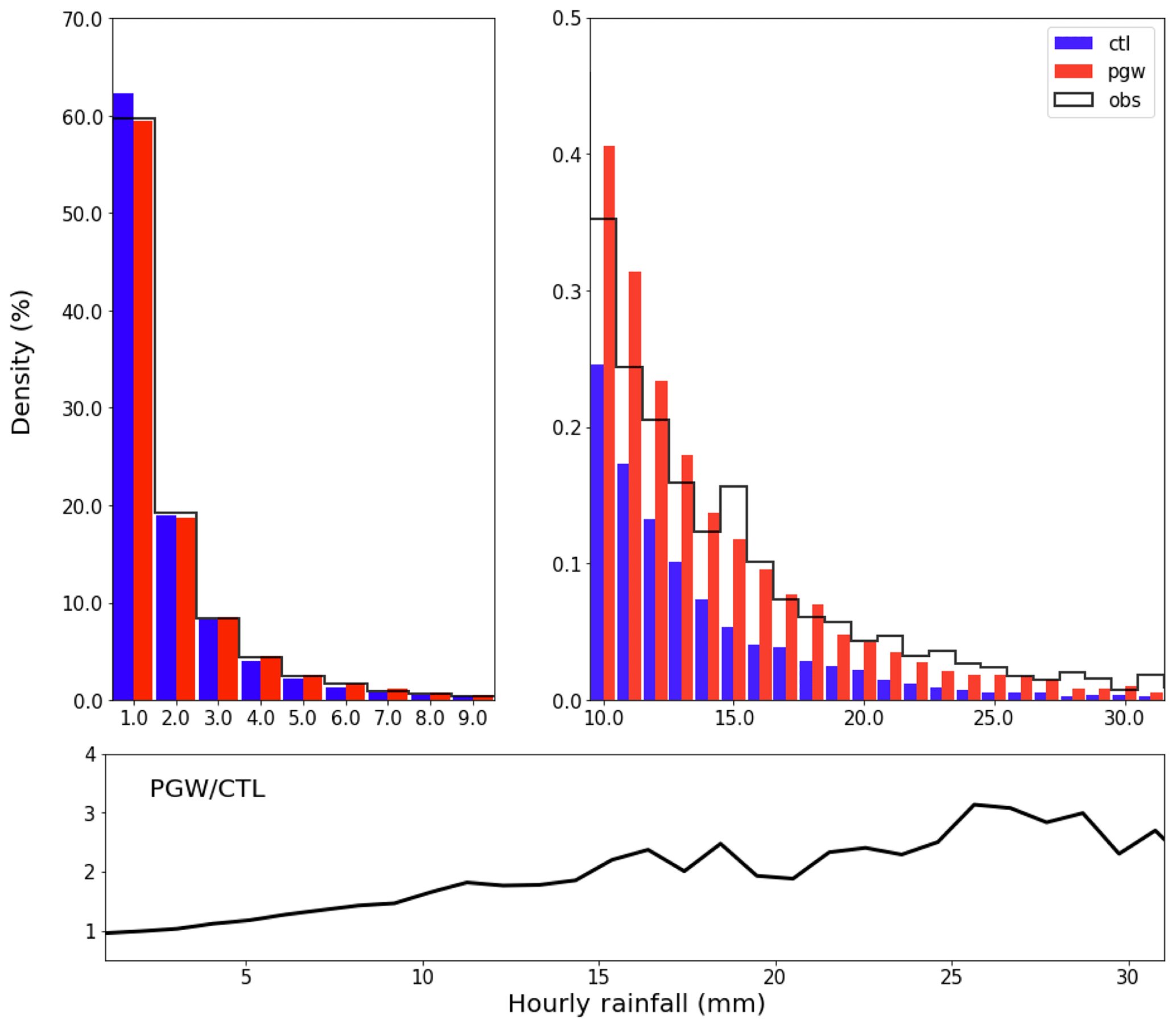
Figure 14Hourly extreme precipitation frequency density over western Canada from station observation, WRF-CTL and PGW. The bottom panel shows the ratio between PGW and CTL for events with different intensities.
For the SRB, the WRF-CTL agrees well with observation in spring, summer, and autumn in terms of moderate to extreme 3 h precipitation events, but significantly underestimates the extreme precipitation events in winter. In spring, autumn, and winter WRF-PGW shows significant increases in extreme precipitation events. In summer WRF-PGW shows a small decrease in precipitation events at 5 mm/3 h and only moderate increases for higher rates. It is also worth mentioning that extreme events are much more numerous in the SRB than in the MRB, especially in spring and summer because the seasonal mean precipitation is higher in the SRB.
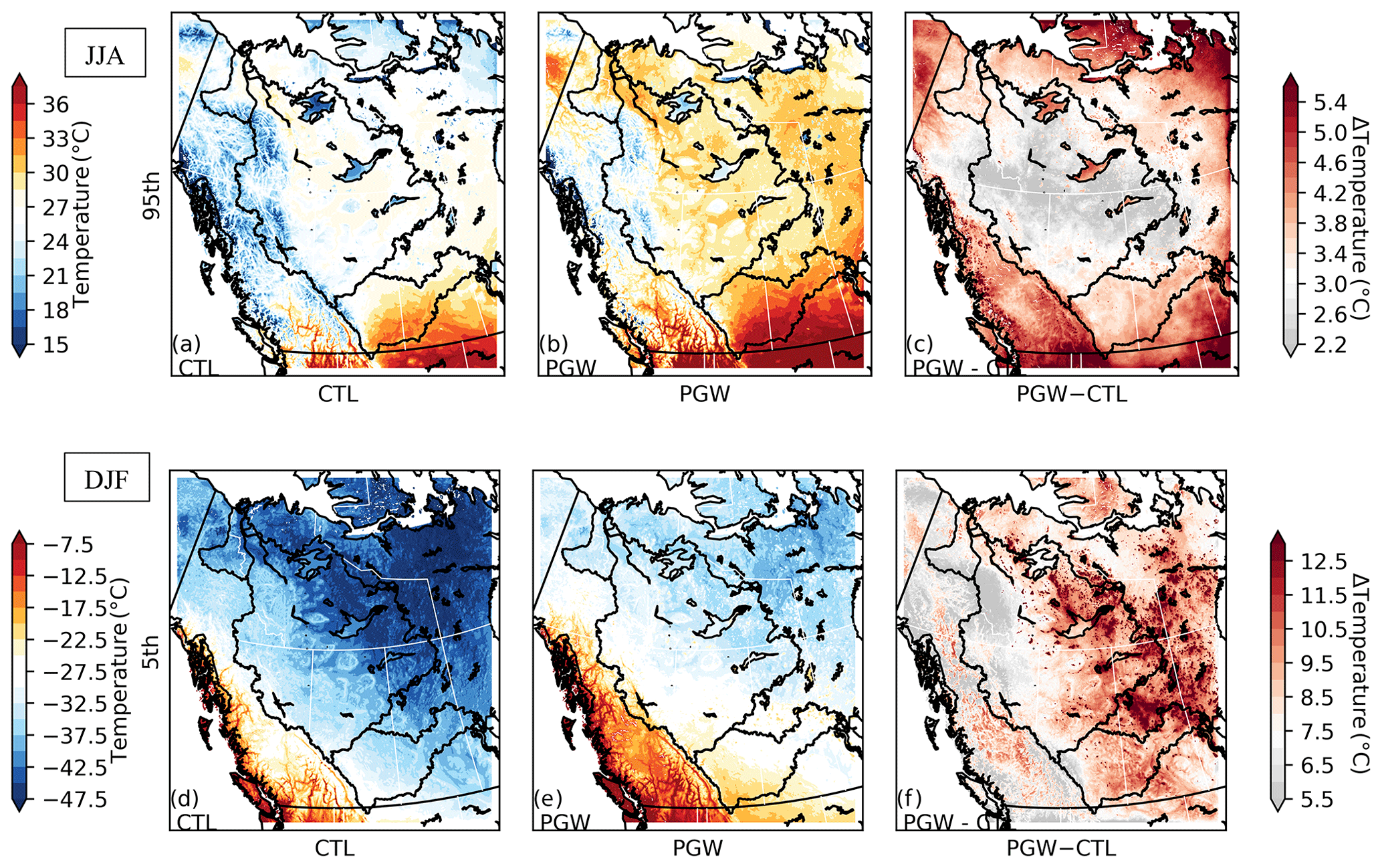
Figure 15(a–c) Extreme statistics of daily maximum temperature in summer WRF-CTL vs. WRF-PGW, 95th percentile. (d–f) Extreme statistics of daily minimum temperature in winter WRF-CTL vs. WRF-PGW, 5th percentile.
Figure 14 shows the changes in hourly precipitation distribution between surface observation and WRF simulations at a 1 h interval. The black line represents observation data collected from 232 surface stations in the SRB and MRB from Environment Climate Change Canada (Website: http://climate.weather.gc.ca/index_e.html, last access: 18 December 2018). The blue and red bars are the closest grid points to these stations extracted every hour (in total 113 952 time steps in 13 years) from the WRF domain for CTL and PGW runs, respectively. Despite the spatial scarcity and data quality associated with station observation, the results do provide some evaluation of the WRF-simulated hourly rainfall, from small to extreme. The majority of hourly precipitation simulated by WRF-CTL is close to that in observations, within the range of 1–10 mm h−1. In this range, future rainfall shows little increase compared to that under the current climate, with even a slight decrease in the amount of light rainfall. The higher hourly rainfall at the high end of the distribution (>10 mm h−1), although comprising only 0.5 % of density in total events, shows a dramatic increase by a probability of 1.5 to 3 times in frequency in the future warmer climate. Notably, the density in the high-end distribution is much higher in the station observation than in CTL because the denominator for observed density, the total number of events, is significantly less in observation, although the absolute number of high-intensity events is comparable or higher in WRF-CTL. In addition to a greater likelihood of the high end of extreme rainfall occurring, a slight decrease in light rainfall is also evident, supporting previous findings from other modeling studies (Cubasch et al., 2013; Easterling et al., 2000; Karl et al., 2006).
In recent decades, there has been an increase in the number of hot extremes in Canada, particularly an increase in nighttime temperature in summer as the global mean temperature rises. Both extreme cold and hot days greatly affect the economy, society, and the daily lives of people. The changes in the high/low percentile values in the temperatures of WRF-PGW and CTL are used to assess the future change in the extreme hot days in summer and cold temperatures in winter in western Canada. The 95th (5th) percentile of the daily maximum (minimum) temperature for CTL, PGW, and their changes in summer (winter) are shown in Fig. 15. We only show the 95th (5th) percentile here as the patterns of warming for the 90th (1st) to 99th (10th) percentiles are similar in summer (winter). The least warming occurs over the central part of the domain where boreal forests are found, mostly within the MRB with a magnitude of about 2.5 ∘C. Over the surrounding area, the warming is stronger, with 4–5 ∘C for the 95th percentile. The change in the 5th percentile of the daily minimum temperature in winter in WRF-PGW relative to WRF-CTL is shown in the bottom row of Fig. 15. In winter the strongest warming for the low percentile Tmin occurs in the eastern domain, where the general warming is also stronger.

Figure 16Extreme statistics of daily precipitation in summer (a) and winter (b) for WRF-CTL vs. WRF-PGW, from top to bottom: 90th, 95th, and 99th percentiles.
The high-percentile daily precipitation distribution in CTL and PGW simulation shows different geographical patterns for different percentiles in summer. The 90th, 95th, and 99th percentiles have typical values of around 10, 18, and 36 mm d−1 in the high-precipitation region, respectively. Compared to CTL, the 90th percentile of daily precipitation in PGW in summer experiences little change in the majority of the domain except for an increase (1.5–3 mm d−1) in the Yukon and western MRB and a small decrease (−1.5 mm d−1) in the southeastern domain, as shown in the first row in Fig. 16a. The 95th percentile of PGW shows a more widespread increase in precipitation by 1–3 mm d−1, compared to CTL, except for a small strip of decreased precipitation east of the SRB, as shown in the second row of Fig. 16a. The 99th percentile of daily summer precipitation shows a consistent increase of 6–9 mm d−1 and about a 15 %–30 % increase across the domain. An extremely high percentile such as 99 % is usually associated with synoptic weather systems, for which the increase in precipitation is more uniform over the domain as it is proportional to vapor loading. The 90th percentile for summer precipitation, about 6–10 mm d−1 over the Canadian Prairies for CTL, can be associated with strong local thunderstorms, which will be strongly affected by boundary layer changes and lower atmospheric conditions in the future. Local water availability and partitioning between sensible and latent heat flux can change the convective inhibition and available convective potential energy, in turn affecting the convective precipitation. Therefore, there is large inhomogeneity of 90th percentile summer precipitation over the domain compared to the higher percentiles.
In winter the relative changes (PGW–CTL) in high-percentile daily precipitation are similar for all the percentiles as shown in Fig. 16b. The change in amount for each percentile follows the general pattern of high daily precipitation distribution in winter: it is concentrated along the coastal mountains in the west and in the Canadian Rockies. In terms of percentage increase, the largest increase is in the northern MRB and the northeastern domain, where precipitation is less than in other parts of the domain. The pattern of the changes in extreme precipitation in winter follows the distribution of mean precipitation, indicating the increase mostly comes from more vapor loading in the atmosphere.
The lack of observation presents challenges for regional climate modeling in several respects. The mountainous terrain and numerous lakes make interpolation of observation data to gridded datasets difficult. Canada's meteorological observation network is heavily concentrated in the southern part of the country and over the plains because of the higher population density and logistical factors. There are far fewer surface observation stations in the sparsely populated area in the north and over the mountainous regions. The sparse observation networks in the regions with low population density provide less reliable and representative observation data to develop and validate regional climate models in the region (Hofstra et al., 2009; Takhsha et al., 2017). As a result, the evaluation of model performance relative to a gridded observation dataset such as ANUSPLIN is less reliable in mountainous and polar regions.
The cold region hydrological cycle and treatment of the snow cover in the land surface model component of RCMs also pose a great challenge to simulate the characteristics of surface temperature and hydrological processes in the region (Casati and Elía, 2014; Niu et al., 2011). For instance, cold region hydrometeorology is strongly affected by snow processes, which are, in turn, affected by fine-scale topography and wind transport. The representation of snow pack and cover in the mountainous region is a challenging obstacle to overcome in realistically reproducing hydro-climatic conditions in the Canadian Rockies (Casati and Elía, 2014; McCrary et al., 2017; Niu et al., 2011). In our case, the near-surface temperature in spring is highly sensitive to the representation of spring snow cover as the snow-albedo feedback can amplify bias in the snow amount in winter to temperature bias in spring.
The convection-permitting high-resolution downscaling by WRF-CTL is in good agreement with CaPA in showing a precipitation pattern with a small wet bias in the northern part of the domain and mountainous region. Notably, however, the regions where WRF-CTL show wet biases also suffer from observation data scarcity or non-representativeness due to orographic precipitation. WRF-PGW projection produces smaller warming in the simulation domain relative to the CMIP5 ensemble mean, especially in the eastern part. WRF-PGW also projects a smaller decrease in summer precipitation over the Canadian Prairies compared to the CMIP5 ensemble, which means the high-resolution simulation tends to generate more summer precipitation than GCMs over the Prairies. In the PGW simulation, the Canadian Prairies, unlike other regions, show a slight decline or no change in total precipitation in summer, especially in moderate intensity precipitation compared to CTL. One reason that there is little to no increase in precipitation in summer may be the decrease in relative humidity in the region, both in the PGW forcing and in the simulation. Dai et al. (2017) showed that a smaller increase in specific humidity than temperature rise can cause a decrease in relative humidity (see the PGW forcing in Fig. 2) as well as a much smaller increase in precipitation. The detailed mechanisms behind the suppression of summer precipitation in the region compared to surrounding regions are currently under investigation.
The high-intensity precipitation events are projected to increase by the end of the 21st century under RCP8.5, as indicated by the notable increase in high-intensity precipitation in the PDF of both the MRB and SRB in WRF-PGW. Extreme precipitation is affected by both water-vapor loading in the atmosphere and changes in vertical velocity, size of storms, translation velocity of storms, etc. Large synoptic-scale storms tend to be affected by vapor loading more than by local-scale circulation, which is consistent with the relative uniformity of the 99th percentile daily precipitation increase across the domain in all seasons. In contrast, large regional differences are seen in the 90th percentile precipitation associated with lesser storms in summer. The hourly precipitation histogram shows a much larger increase in number for heavy precipitation events (about 300 %) vs. light precipitation (about 150 %). Research is ongoing on changes in storm-related characteristics based on an objective storm-tracking algorithm known as MODE-TD.
For many hydrological and agricultural applications, bias correction of temperature and precipitation for RCM outputs often needs to be reconciled with benchmarked parameters or criteria. Various bias-correction methods have been used to bias-correct RCM output before their application. Quantile mapping, in its various forms, tends to project simulated distribution onto the observed distribution and achieve the observed mean and distribution. Due to WRF-CTL's cold bias in spring east of the Canada Rockies and wet bias in the MRB, bias correction based on quantile mapping is recommended for applications calibrated on observed hydroclimate. However, due to shifting in the distribution of hourly precipitation probability in WRF-PGW relative to WRF-CTL, quantile mapping for our PGW simulation alters the precipitation change signal between the original WRF-PGW and WRF-CTL. To preserve the climate change signal in bias correction and to produce properly bias-corrected summer precipitation for future scenarios, the physical processes involved in the change need to be considered.
The 4 km WRF dynamical downscaling of the current and future (RCP8.5) climate provides valuable high-resolution regional climate data for applications in hydrology and climatic impact studies. High-resolution convection-permitting regional climate simulations were conducted using WRF at 4 km grid spacing for western Canada for the current climate (CTL, 2000–2015) and a high-end emission scenario, RCP8.5, through the PGW approach. The WRF-CTL simulation is forced with ERA-Interim reanalysis at 6 h intervals on the boundary. The WRF-PGW's forcing is the same as that of CTL plus the climate change signals derived from an ensemble of 19 CMIP5 members from 2070 to 2100 and from 1976 to 2005. At a 4 km horizontal resolution, the convection in the model is explicitly resolved and the convective parameterization schemes are disabled.
The evaluation of WRF-CTL against the ANUSPLIN gridded observation dataset and reanalyses such as CaPA and NARR shows good agreement between WRF-CTL and the reference datasets in terms of geographical distribution, seasonal cycle, and interannual variation. For temperature bias, the largest bias occurs over the plains east of the Rockies in spring. In general, WRF-CTL produces more precipitation than both ANUSPLIN and CaPA, especially in the northern part of domain where there are few observations and over terrains where most observation sites are at a lower elevation and less representative than desired. The precipitation bias of WRF-CTL against CaPA is less than that vs. ANUSPLIN, which has been shown to be too dry in the northern domain and SRB (Wong et al., 2017). The evaluation reminds us that many discrepancies are due to poor coverage of observation data that were interpolated to data-sparse regions. It shows the urgent need for high-quality and reasonable geographical coverage of meteorological observation over Canada to provide both forcing for RCM simulation and validation data for model performance.
In a future warming scenario, WRF-PGW shows substantial warming across western Canada under the RCP.8.5 emission scenario, though the warming is slightly less than that from the CMIP5 ensemble projection. The warming is stronger in the cold season, especially over the northeastern polar region in winter and over the Canadian Prairies in spring. While precipitation changes in PGW over CTL vary with the seasons, in both basins, more increases occur in spring and late autumn, whereas precipitation in the SRB in summer either shows no increase (remains at zero) or decreases. The smallest change in precipitation occurs in summer, when parts of the Prairies receive less precipitation in PGW than in CTL. With almost no increase in summer precipitation and much larger evapotranspiration in PGW than in CTL, the Canadian Prairies will experience water availability challenges during the growing season. With the large temperature increase and potential increased evaporation, the small increase/decrease in summer precipitation indicates that the Canadian Prairies and the southern boreal forest biomes will see a slight decline in effective precipitation in summer, which will likely have a significant impact on soil moisture for farming and forest fire occurrences. This dynamic downscaling by WRF is also different from CMIP5 ensemble mean projection for the SRB and southern MRB, where a significant decline in summer precipitation is projected. As convection plays an important role in summer precipitation over the Canadian Prairies, the difference between the 4 km WRF and the GCM ensemble may be due to the difference in simulating convection. There is also more increase in the projected precipitation change over the British Columbia coast and Canadian Rockies in WRF than in CMIP5, which results from the representation of the underlying topography and lack of orographic lifting in the GCM relative to 4 km WRF.
As the warmer atmosphere holds more water vapor, WRF-PGW shows an increase in precipitation over WRF-CTL. Severe precipitation events increase more than moderate and light precipitation events as the distribution of precipitation events shifts toward more higher-intensity events in all seasons except summer. In summer, light to moderate precipitation (5–10 mm/3 h) in WRF-PGW actually decreases compared to WRF-CTL in both the MRB and SRB. The increase in precipitation in cold seasons is larger in terms of percentage in the northeast, where greater warming is expected. Due to this shift in precipitation intensity to the higher end in the PGW simulation, the seemingly moderate increase in total precipitation in summer for both basins may not reflect the real change in flooding risk and water availability for agriculture because the frequency of extreme precipitation events increases disproportionately. The shift in the precipitation intensity distribution in WRF-PGW also poses challenges, for bias correction relies on fitting an observed distribution.
In summary, the high-resolution convection-permitting WRF simulations are shown to reproduce the general characteristics of the regional climate in western Canada. The model results provide bountiful opportunities for not only atmospheric and climate scientists interested in local–regional-scale meteorological phenomena and dynamics and circulation changes under global warming, but also stakeholders in hydrology and agriculture who need high-resolution climate information and detailed global warming projections for western Canada.
The WRF simulation over western Canada can be accessed at https://tuna.cs.uwaterloo.ca (last acces: October 2019). The ANUSPLIN data can be downloaded at ftp://ftp.nrcan.gc.ca/pub/outgoing/canada_daily_grids/ (last access: October 2019). The NARR data were downloaded from https://www.esrl.noaa.gov/psd/data/gridded/data.narr.html (last access: October 2019). The CaPA data can be accessed at https://weather.gc.ca/grib/grib2_RDPA_ps10km_e.html (last access: October 2019).
The supplement related to this article is available online at: https://doi.org/10.5194/hess-23-4635-2019-supplement.
YL designed the experiments and CL, ZZ, SK, ZL performed the simulations. ZL, ZZ conducted the analysis and prepared the figures with the helps from YL, LS, and PX. YL and ZL prepared the manuscript with contributions from all the co-authors.
The authors declare that they have no conflict of interest.
This article is part of the special issue “Understanding and predicting Earth system and hydrological change in cold regions”. It is not associated with a conference.
The authors gratefully acknowledge the support from the Changing Cold Regions Network (CCRN) funded by the Natural Science and Engineering Research Council of Canada (NSERC), as well as the Global Water Future project and Global Institute of Water Security at the University of Saskatchewan. Yanping Li acknowledges the support from a NSERC Discovery Grant.
This research has been supported by the Natural Sciences and Engineering Research Council of Canada (projects Changing Cold Regions Network (CCRN) and Global Water Future).
This paper was edited by John Hanesiak and reviewed by two anonymous referees.
Bindoff, N., Stott, P., Achuta Rao, K., Allen, M., Gillett, N., Gutzler, D., Hansingo, K., Hegerl, G., Hu, Y., Jain, S., Mokhov, I., Overland, J., Perlwitz, J., Sebbari, R., and Zhang, X.: Detection and attribution of climate change: From global to regional, in: Climate change 2013: The physical science basis, Contribution of working group i to the fifth assessment report of the intergovernmental panel on climate change, edited by: Stocker, T., Qin, D., Plattner, G.-K., Tignor, M., Allen, S., Boschung, J., Nauels, A., Xia, Y., Bex, V., and Midgley, P., Cambridge University Press, Cambridge, UK and New York, NY, USA, 867–952, 2013.
Bonsal, B. R., Aider, R., Gachon, P., and Lapp, S.: An assessment of canadian prairie drought: Past, present, and future, Clim. Dynam., 41, 501–516, https://doi.org/10.1007/s00382-012-1422-0, 2013.
Casati, B. and de Elía, R.: Temperature extremes from canadian regional climate model (crcm) climate change projections, Atmos.-Ocean, 52, 191–210, https://doi.org/10.1080/07055900.2014.886179, 2014.
Castro, C. L.: Dynamical downscaling: Assessment of value retained and added using the regional atmospheric modeling system (rams), J. Geophys. Res., 110, D05108, https://doi.org/10.1029/2004jd004721, 2005.
Chen, F. and Dudhia, J.: Coupling an advanced land surface-hydrology model with the penn state-ncar mm5 modeling system. Part i: Model implementation and sensitivity, Mon. Weather Rev., 129, 569–585, https://doi.org/10.1175/1520-0493(2001)129<0569:CAALSH>2.0.CO;2, 2001.
Collins, W. D., Rasch, P., Boville, B., Hack, J., McCaa, J., Williamson, D., Kiehl, J., Briegleb, B., Bitz, C., Lin, S.-J., Zhang, M., and Dai, Y.: Description of the NCAR community atmosphere model (cam 3.0), Natl. Cent. for Atmos. Res., Boulder, Colorado, 2004.
Cubasch, U., Wuebbles, D., Chen, D., Facchini, M., Frame, D., Mahowald, N., and Winther, J.-G.: Introduction, in: Climate change 2013: The physical science basis, Contribution of working group i to the fifth assessment report of the intergovernmental panel on climate change, edited by: Stocker, T., Qin, D., Plattner, G.-K., Tignor, M., Allen, S., Boschung, J., Nauels, A., Xia, Y., Bex, V., and Midgley, P., Cambridge University Press, Cambridge, UK and New York, NY, USA, 119–158, 2013.
Dai, A., Rasmussen, R. M., Liu, C., Ikeda, K., and Prein, A. F.: A new mechanism for warm-season precipitation response to global warming based on convection-permitting simulations, Clim. Dynam., https://doi.org/10.1007/s00382-017-3787-6, in press, 2017.
Dee, D. P., Uppala, S. M., Simmons, A. J., Berrisford, P., Poli, P., Kobayashi, S., Andrae, U., Balmaseda, M. A., Balsamo, G., Bauer, P., Bechtold, P., Beljaars, A. C. M., van de Berg, L., Bidlot, J., Bormann, N., Delsol, C., Dragani, R., Fuentes, M., Geer, A. J., Haimberger, L., Healy, S. B., Hersbach, H., Hólm, E. V., Isaksen, L., Kållberg, P., Köhler, M., Matricardi, M., McNally, A. P., Monge-Sanz, B. M., Morcrette, J.-J., Park, B.-K., Peubey, C., de Rosnay, P., Tavolato, C., Thépaut, J.-N., and Vitart, F.: The ERA-Interim reanalysis: Configuration and performance of the data assimilation system, Q. J. Roy. Meteorol. Soc., 137, 553–597, https://doi.org/10.1002/qj.828, 2011.
Deser, C., Phillips, A., Bourdette, V., and Teng, H.: Uncertainty in climate change projections: The role of internal variability, Clim. Dynam., 38, 527–546, https://doi.org/10.1007/s00382-010-0977-x, 2012.
Easterling, D. R., Meehl, G. A., Parmesan, C., Changnon, S. A., Karl, T. R., and Mearns, L. O.: Climate extremes: Observations, modeling, and impacts, Science, 289, 2068–2074, 2000.
Eum, H.-I., Gachon, P., Laprise, R., and Ouarda, T.: Evaluation of regional climate model simulations versus gridded observed and regional reanalysis products using a combined weighting scheme, Clim. Dynam., 38, 1433–1457, https://doi.org/10.1007/s00382-011-1149-3, 2012.
Eum, H.-I., Dibike, Y., Prowse, T., and Bonsal, B.: Inter-comparison of high-resolution gridded climate data sets and their implication on hydrological model simulation over the athabasca watershed, canada, Hydrol. Process., 28, 4250–4271, https://doi.org/10.1002/hyp.10236, 2014.
Feser, F., Rockel, B., von Storch, H., Winterfeldt, J., and Zahn, M.: Regional Climate Models Add Value To Global Model Data: A Review and Selected Examples, B. Am. Meteorol. Soc., 92, 1181–1192, https://doi.org/10.1175/2011bams3061.1, 2011.
Fortin, V., Roy, G., Stadnyk, T., Koenig, K., Gasset, N., and Mahidjiba, A.: Ten years of science based on the canadian precipitation analysis: A capa system overview and literature review, Atmos.-Ocean, 56, 178–196, https://doi.org/10.1080/07055900.2018.1474728, 2018.
Giorgi, F., Jones, C., and Asrar, G. R.: Addressing climate information needs at the regional level: The cordex framework, WMO Bulletin, 58, 175–183, 2009.
Hofstra, N., New, M., and McSweeney, C.: The Influence of Interpolation and Station Network Density on the Distributions and Trends of Climate Variables in Gridded Daily data, Clim. Dynam., 35, 841–858, https://doi.org/10.1007/s00382-009-0698-1, 2009.
Hopkinson, R. F., McKenney, D. W., Milewska, E. J., Hutchinson, M. F., Papadopol, P., and Vincent, L. A.: Impact of aligning climatological day on gridding daily maximum–minimum temperature and precipitation over canada, J. Appl. Meteorol. Clim., 50, 1654–1665, https://doi.org/10.1175/2011JAMC2684.1, 2011.
Hutchinson, M. F., McKenney, D. W., Lawrence, K., Pedlar, J. H., Hopkinson, R. F., Milewska, E., and Papadopol, P.: Development and testing of canada-wide interpolated spatial models of daily minimum-maximum temperature and precipitation for 1961–2003, J. Appl. Meteorol. Clim., 48, 725–741, https://doi.org/10.1175/2008jamc1979.1, 2009.
IPCC: Climate change 2013: The physical science basis, in: Contribution of working group i to the fifth assessment report of the intergovernmental panel on climate change, Book, Cambridge University Press, Cambridge, UK and New York, NY, USA, 2013.
Karl, T. R., Meehl, G. A., Peterson, T. C., Kunkel, K. E., Gutowski Jr., W. J., and Easterling, D. R.: Executive Summary in Weather and Climate Extremes in a Changing Climate, in: Regions of Focus: North America, Hawaii, Caribbean, and U.S. Pacific Islands, edited by: Karl, T. R., Meehl, G. A., Miller, C. D., Hassol, S. J., Waple, A. M., and Murray, W. L., A Report by the US Climate Change Science Program and the Subcommittee on Global Change Research, Washington, D.C., 2008.
Li, Y., K. Szeto, K., Stewart, R. E., Thériault, J. M., Chen, L., Kochtubajda, B., Liu, A., Boodoo, S., Goodson, R., Mooney, C., and Kurkute, S.: A Numerical Study of the June 2013 Flood – Producing Extreme Rainstorm over Southern Alberta, J. Hydrometeorol., 18, 2057–2078, https://doi.org/10.1175/JHM-D-15-0176.1, 2017.
Liu, C., Ikeda, K., Thompson, G., Rasmussen, R., and Dudhia, J.: High-resolution simulations of wintertime precipitation in the colorado headwaters region: sensitivity to physics parameterizations, Mon. Weather Rev., 139, 3533–3553, https://doi.org/10.1175/MWR-D-11-00009.1, 2011.
Liu, C., Ikeda, K., Rasmussen, R., Barlage, M., Newman, A. J., Prein, A. F., Chen, F., Chen, L., Clark, M., Dai, A., Dudhia, J., Eidhammer, T., Gochis, D., Gutmann, E., Kurkute, S., Li, Y., Thompson, G., and Yates, D.: Continental-Scale Convection-Permitting Modeling of the Current and Future Climate of North America, Clim. Dynam., 49, 71–95, https://doi.org/10.1007/s00382-016-3327-9, 2017.
Mahfouf, J.-F., Brasnett, B., and Gagnon, S.: A Canadian precipitation analysis (CaPA) project: Description and preliminary results, Atmos.-Ocean, 45, 1–17, https://doi.org/10.3137/ao.450101, 2007.
McCrary, R. R., McGinnis, S., and Mearns, L. O.: Evaluation of Snow Water Equivalent in Narccap Simulations, Including Measures of Observational Uncertainty, J. Hydrometeorol., 18, 2425–2452, https://doi.org/10.1175/JHM-D-16-0264.1, 2017.
Mearns, L. O., Gutowski, W., Jones, R., Leung, R., McGinnis, S., Nunes, A., and Qian, Y.: A Regional Climate Change Assessment Program for North America, Eos Trans. Am. Geophys. Union, 90, 311–311, https://doi.org/10.1029/2009EO360002, 2009.
Mearns, L. O., Sain, S., Leung, L. R., Bukovsky, M. S., McGinnis, S., Biner, S., Caya, D., Arritt, R. W., Gutowski, W., Takle, E., Snyder, M., Jones, R. G., Nunes, A. M. B., Tucker, S., Herzmann, D., McDaniel, L., and Sloan, L.: Climate change projections of the north american regional climate change assessment program (narccap), Climatic Change, 120, 965–975, https://doi.org/10.1007/s10584-013-0831-3, 2013.
Mearns, L. O., Lettenmaier, D. P., and McGinnis, S.: Uses of results of regional climate model experiments for impacts and adaptation studies: The example of NARCCAP, Curr. Clim. Change Rep., 1, 1–9, https://doi.org/10.1007/s40641-015-0004-8, 2015.
Meng, X., Lyu, S., Zhang, T., Zhao, L., Li, Z., Han, B., Li, S., Ma, D., Chen, H., Ao, Y., Luo, S., Shen, Y., Guo, J., and Wen, L.: Simulated Cold Bias Being Improved By Using Modis Time-Varying Albedo in the Tibetan Plateau in WRF model, Environ. Res. Lett., 13, 044028, https://doi.org/10.1088/1748-9326/aab44a, 2018.
Mesinger, F., DiMego, G., Kalnay, E., Mitchell, K., Shafran, P. C., Ebisuzaki, W., Jovic ́, D., Woollen, J., Rogers, E., Berbery, E. H., Ek, M. B., Fan, Y., Grumbine, R., Higgins, W., Li, H., Lin, Y., Manikin, G., Parrish, D., and Shi, W.: North american regional reanalysis, B. Am. Meteorol. Soc., 87, 343–360, https://doi.org/10.1175/bams-87-3-343, 2006.
Misra, V. and Kanamitsu, M.: Anomaly nesting: a methodology to downscale seasonal climate simulations from agcms, J. Climate, 17, 3249–3262, https://doi.org/10.1175/1520-0442(2004)017<3249:anamtd>2.0.co;2, 2004.
Morrison, H., Thompson, G., and Tatarskii, V.: Impact of cloud microphysics on the development of trailing stratiform precipitation in a simulated squall line: comparison of one- and two-moment schemes, Mon. Weather Rev., 137, 991–1007, https://doi.org/10.1175/2008mwr2556.1, 2009.
Musselman, K. N., Lehner, F., Ikeda, K., Clark, M. P., Prein, A. F., Liu, C., Barlage, M., and Rasmussen, R.: Projected increases and shifts in rain-on-snow flood risk over western north america, Nat. Clim. Change, 8, 808–812, https://doi.org/10.1038/s41558-018-0236-4, 2018.
Nelson, B. R., Prat, O. P., Seo, D., and Habib, E.: Assessment and Implications of NCEP Stage IV Quantitative Precipitation Estimates for Product Intercomparisons, Weather Forecast., 31, 371–394, https://doi.org/10.1175/WAF-D-14-00112.1, 2016.
Niu, G.-Y., Yang, Z.-L., Mitchell, K. E., Chen, F., Ek, M. B., Barlage, M., Kumar, A., Manning, K., Niyogi, D., Rosero, E., Tewari, M., and Xia, Y.: The community noah land surface model with multiparameterization options (noah-mp): 1. Model description and evaluation with local-scale measurements, J. Geophys. Res., 116, D12109, https://doi.org/10.1029/2010jd015139, 2011.
Prein, A. F., Langhans, W., Fosser, G., Ferrone, A., Ban, N., Goergen, K., Keller, M., Tölle, M., Gutjahr, O., Feser, F., Brisson, E., Kollet, S., Schmidli, J., van Lipzig, N. P. M., and Leung, R.: A Review on Regional Convection-Permitting Climate Modeling: Demonstrations, Prospects, and challenges, Rev. Geophys., 53, 323–361, https://doi.org/10.1002/2014RG000475, 2015.
Prein, A. F., Liu, C., Ikeda, K., Bullock, R., Rasmussen, R. M., Holland, G. J., and Clark, M.: Simulating north american mesoscale convective systems with a convection-permitting climate model, Clim. Dynam., https://doi.org/10.1007/s00382-017-3993-2, in press, 2017a.
Prein, A. F., Rasmussen, R. M., Ikeda, K., Liu, C., Clark, M. P., and Holland, G. J.: The future intensification of hourly precipitation extremes, Nat. Clim. Change, 7, 48–52, https://doi.org/10.1038/nclimate3168, 2017b.
Rasmussen, K. L., Prein, A. F., Rasmussen, R. M., Ikeda, K., and Liu, C.: Changes in the convective population and thermodynamic environments in convection-permitting regional climate simulations over the United States, Clim. Dynam., https://doi.org/10.1007/s00382-017-4000-7, 2017.
Rasmussen, R., Liu, C., Ikeda, K., Gochis, D., Yates, D., Chen, F., Tewari, M., Barlage, M., Dudhia, J., Yu, W., Miller, K., Arsenault, K., Grubišić, V., Thompson, G., and Gutmann, E.: High-resolution coupled climate runoff simulations of seasonal snowfall over colorado: A process study of current and warmer climate, J. Climate, 24, 3015–3048, https://doi.org/10.1175/2010JCLI3985.1, 2011.
Rasmussen, R., Ikeda, K., Liu, C., Gochis, D., Clark, M., Dai, A., Gutmann, E., Dudhia, J., Chen, F., Barlage, M., Yates, D., and Zhang, G.: Climate change impacts on the water balance of the colorado headwaters: High-resolution regional climate model simulations, J. Hydrometeorol., 15, 1091–1116, https://doi.org/10.1175/jhm-d-13-0118.1, 2014.
Sato, T., Kimura, F., and Kitoh, A.: Projection of global warming onto regional precipitation over mongolia using a regional climate model, J. Hydrol., 333, 144–154, https://doi.org/10.1016/j.jhydrol.2006.07.023, 2007.
Stralberg, D., Wang, X., Parisien, M.-A., Robinne, F.-N., Sólymos, P., Mahon, C. L., Nielsen, S. E., and Bayne, E. M.: Wildfire-mediated vegetation change in boreal forests of alberta, canada, Ecosphere, 9, e02156, https://doi.org/10.1002/ecs2.2156, 2018.
Sugiyama, M., Shiogama, H., and Emori, S.: Precipitation extreme changes exceeding moisture content increases in miroc and ipcc climate models, P. Natl. Acad. Sci. USA, 107, 571–575, https://doi.org/10.1073/pnas.0903186107, 2009.
Takhsha, M., Nikiéma, O., Lucas-Picher, P., Laprise, R., Hernández-Díaz, L., and Winger, K.: Dynamical downscaling with the fifth-generation canadian regional climate model (crcm5) over the cordex arctic domain: Effect of large-scale spectral nudging and of empirical correction of sea-surface temperature, Clim. Dynam., 51, 161–186, https://doi.org/10.1007/s00382-017-3912-6, 2017.
Thompson, G., Field, P. R., Rasmussen, R. M., and Hall, W. D.: Explicit forecasts of winter precipitation using an improved bulk microphysics scheme. Part ii: Implementation of a new snow parameterization, Mon. Weather Rev., 136, 5095–5115, https://doi.org/10.1175/2008mwr2387.1, 2008.
Trenberth, K. E., Dai, A., Rasmussen, R. M., and Parsons, D. B.: The changing character of precipitation, B. Am. Meteorol. Soc., 84, 1205–1218, https://doi.org/10.1175/bams-84-9-1205, 2003.
Westra, S., Fowler, H. J., Evans, J. P., Alexander, L. V., Berg, P., Johnson, F., Kendon, E. J., Lenderink, G., and Roberts, N. M.: Future changes to the intensity and frequency of short-duration extreme rainfall, Rev. Geophys., 52, 522–555, https://doi.org/10.1002/2014rg000464, 2014.
Weusthoff, T., Ament, F., Arpagaus, M., and Rotach, M. W.: Assessing the benefits of convection-permitting models by neighborhood verification: Examples from map d-phase, Mon. Weather Rev., 138, 3418–3433, https://doi.org/10.1175/2010mwr3380.1, 2010.
Wong, J. S., Razavi, S., Bonsal, B. R., Wheater, H. S., and Asong, Z. E.: Inter-comparison of daily precipitation products for large-scale hydro-climatic applications over canada, Hydrol. Earth Syst. Sci., 21, 2163–2185, https://doi.org/10.5194/hess-21-2163-2017, 2017.
Xie, S.-P. and Kosaka, Y.: What caused the global surface warming hiatus of 1998-2013?, Curr. Clim. Change Rep., 3, 128–140, https://doi.org/10.1007/s40641-017-0063-0, 2017.
Xu, T. and Hutchinson, M. F.: New developments and applications in the ANUCLIM spatial climatic and bioclimatic modelling package, Environ. Model. Softw., 40, 267–279, https://doi.org/10.1016/j.envsoft.2012.10.003, 2013.
- Abstract
- Introduction
- Model setup and data
- Evaluation of the CTL experiment
- Pseudo-global warming simulation
- Extreme temperature and precipitation
- Discussion
- Summary
- Data availability
- Author contributions
- Competing interests
- Special issue statement
- Acknowledgements
- Financial support
- Review statement
- References
- Supplement