Modelling of the shallow water table at high spatial resolution using random forests

Machine learning provides great potential for modelling hydrological variables at a spatial resolution beyond the capabilities of physically based modelling. This study features an application of random forests (RF) to model the depth to the shallow water table, for a wintertime minimum event, at a 50 m resolution over a 15 000 km² domain in Denmark. In Denmark, the shallow groundwater poses severe risks with respect to groundwater-induced flood events, affecting both urban and agricultural areas. The risk is especially critical in wintertime, when the shallow groundwater is close to terrain. In order to advance modelling capabilities of the shallow groundwater system and to provide estimates at the scales required for decision-making, this study introduces a simple method to unify RF and physically based modelling. Results from the national water resources model in Denmark (DK-model) at a 500 m resolution are employed as covariates in the RF model. Thus, RF ensures physical consistency at a coarse scale and fully exhausts high-resolution information from readily available environmental variables. The vertical distance to the nearest water body was rated as the most important covariate in the trained RF model followed by the DK-model. The evaluation test of the trained RF model was very satisfying with a mean absolute error of 76 cm and a coefficient of determination of 0.56. The resulting map underlines the severity of groundwater flooding risk in Denmark, as the average depth to the shallow groundwater is 1.9 m and approximately 29 % of the area is characterized as having a depth of less than 1 m during a typical wintertime minimum event. This study brings forward a novel method for assessing the spatial patterns of covariate importance of the RF predictions that contributes to an increased interpretability of the RF model. Quantifying the uncertainty of RF models is still rare for hydrological applications. Two approaches, namely random forests regression kriging (RFRK) and quantile regression forests (QRF), were tested to estimate uncertainties related to the predicted groundwater levels.

1 Introduction

The shallow groundwater, defined as the uppermost water table, is a key state variable of the hydrological cycle that has a wide range of vital implications for human health, terrestrial ecosystems, food security and energy production (Gleeson et al., 2016). Following Fan et al. (2013), up to one-third of the global land area is affected by shallow groundwater, being either directly groundwater-fed or having the water table or capillary fringe within plant rooting depths. In many regions of the world, groundwater aquifers are being depleted extensively by unsustainable anthropogenic activities (Richey et al., 2015). In addition, climate change affects groundwater recharge and storage, which, in many cases, impacts the resilience of shallow groundwater systems (Ferguson and Maxwell, 2010; Rodell et al., 2018).

Shallow groundwater has a broad relevance that expands beyond hydrological science. For instance, Kahlown et al. (2005) and Zipper et al. (2015) studied the dependency between crop yield and the water table. They concluded that groundwater played an essential role in meeting the crop water requirements in many agricultural settings. However, water tables too close to the surface resulted in reduced yields, and both studies identified an optimal water table height of between 1 and 2 m below the surface. Moreover, several studies have highlighted the controlling mechanisms that the water table has on the energy balance at the land surface, inferring a link to the latent heat flux and the delineation of water- and energy-limited ecosystems (Kollet and Maxwell, 2008; Maxwell and Condon, 2016). Other studies stressed the connections between groundwater and the near-surface climate via coupled numerical modelling experiments (Larsen et al., 2016; Wang et al., 2018). Shallow groundwater is also of importance in urban contexts (Bricker et al., 2017), with special focus on urban flooding which can be directly induced or indirectly intensified by high groundwater levels (Jankowfsky et al., 2014; Kreibich and Thieken, 2008; MacDonald et al., 2012). Moreover, MacDonald et al. (2010) and Upton and Jackson (2011) studied the underlying processes, estimated return periods and mapped risk of groundwater flooding events.

In Denmark, the quantitative status of shallow groundwater systems is challenged by climate change and groundwater abstraction (Henriksen et al., 2008; Karlsson et al., 2016). In more detail, Kidmose et al. (2013) demonstrated that groundwater levels are expected to rise by up to 1.5 m for a 100-year event relative to present average conditions. Similar findings were presented by van Roosmalen et al. (2007), who quantified regional differences across Denmark in the projected change of groundwater levels depending on soil types with more profound increases in highly permeable sandy soils. Moreover, Henriksen et al. (2012) analysed climate change effects on the shallow water table over Denmark for mean and maximum conditions for nine different climate models and identified changes of at least 0.5 m for 26 % of Denmark. This finding represented the median change across the nine applied climate models.

The above-mentioned problems call for comprehensive modelling tools that can support environmental decision-making aiming at tackling current and future challenges related to shallow groundwater. Spatial scales that are relevant for society and required for adequate decision-making can typically not be provided by numerical, physically based models alone. This limitation is mainly related to the fact that such models are computationally very expensive which hinders thorough conduct calibration, sensitivity and uncertainty analysis at high resolution (Asher et al., 2015; Stisen et al., 2018). Furthermore, it is difficult to parameterize subsurface processes regardless the scale (Beven et al., 2015). Moreover, the wealth and detail of hydrological data are under continual growth (Chaney et al., 2018) and the resulting big data are often not harnessed optimally in existing modelling frameworks (Best et al., 2015; Nearing et al., 2016). As outlined by Reichstein et al. (2019), machine learning will play an essential role in advancing current modelling systems by integrating machine learning and numerical models. The development and testing of such hybrid models, complementing the benefits of physically based models and machine learning, have gradually gained more attention in recent years in the hydrological community. A roadmap toward machine-learning-facilitated discoveries of hydrological systems has been outlined by Shen at al. (2018) and will likely play an eminent role in the future of hydrology. More generally, Karpatne et al. (2017) coined the paradigm “theory-guided data science” which comprises a diverse list of approaches with which physically based models and machine learning can be combined. All three of the above-mentioned references focus on the coupling of physically based models with the versatility of data-driven modelling frameworks. In more detail, they have identified that the interpretability of machine learning models is among the main challenges for the successful adoption of big data technologies in hydrological science.

This study highlights the applicability of machine learning, namely the random forests (RF) algorithm (Breiman, 2001), to model the depth to the shallow groundwater at a regional scale at high spatial resolution. The aim is to produce a map that captures an extreme wintertime condition, representing a minimum depth to the water table. Such an event can potentially induce groundwater flooding that poses risks related to infrastructure and agriculture. Thus, the resulting high-resolution map will be a versatile screening resource for environmental decision-making and climate change adaption planning. The proposed RF model draws on the Danish national water resources model (Højberg et al., 2013) which provides a coarse estimation of the depth to the shallow water table. In this way, the RF model utilizes the coarse prediction of the physically based model to ensure overall physical consistency, which may not be granted by the RF model alone. Hence, this study tests a simple hybrid model integrating the output of a numerical model in a machine learning framework. Before machine learning techniques can be considered as a standard tool for environmental decision-making and planning, methods to conduct comprehensive sensitivity analysis and uncertainty assessment need to be developed and tested thoroughly. In order to advance this field of hydrological research, this study compares two different methods for quantifying the uncertainty of a RF model, namely random forests regression kriging (Hengl et al., 2015) and quantile regression forests (Meinshausen, 2006). Furthermore, this study features a novel methodology to quantify covariate importance, and thereby the sensitivity of the model inputs, which ultimately helps to better comprehend and interpret the RF prediction.

Numerous studies have already successfully employed machine learning techniques to predict the temporal dynamics of the groundwater system based on artificial neural networks (Banerjee et al., 2009; Daliakopoulos et al., 2005; Shiri et al., 2013; Yoon et al., 2011) or other machine learning methods (Fallah-Mehdipour et al., 2013). However, opportunities to utilize data-driven modelling to assess the spatial dimension of the water table have not been fully exhausted to date. Fienen et al. (2013) are among the few that have utilized a machine learning technique to map the depth to the groundwater in space (i.e. Bayesian network). Machine learning has already been applied to model other groundwater-related variables, such as the nitrate concentration (Nolan et al., 2015; Tesoriero et al., 2015), arsenic concentrations (Erickson et al., 2018; Winkel et al., 2011) and redox conditions in the subsurface (Close et al., 2016; Koch et al., 2019), and the potential to map the depth to the water table is tangible.

The four main objectives of this paper are as follows: (1) to train a RF model that is capable of predicting the depth to the shallow water table at a high spatial resolution, (2) to outline a simple and generic method that unifies a physically based model and machine learning, (3) to conduct a comprehensive sensitivity analysis to better interpret the RF model prediction and (4) to assess the uncertainty related to the RF model based on two different approaches.

2 Methods

2.1 Study area

The study area encompasses a large part of the Jutland Peninsula, which is located in Denmark in northern Europe (54.5–57.8^∘ N and 8.0–10.9^∘ E). The extent of the study area amounts to approximately 15 000 km² and its general surficial geological setting is illustrated in Fig. 1. The landscape of Jutland was formed by a sequence of Pleistocene glaciations and postglacial processes. The geology of the eastern part of the study domain is dominated by Weichselian moraine sediments with a moderate clay content, whereas the west is characterized by moraine sediments originating from the Saalian age, referred to as hill islands, intertwined by sandy Weichselian outwash plains.

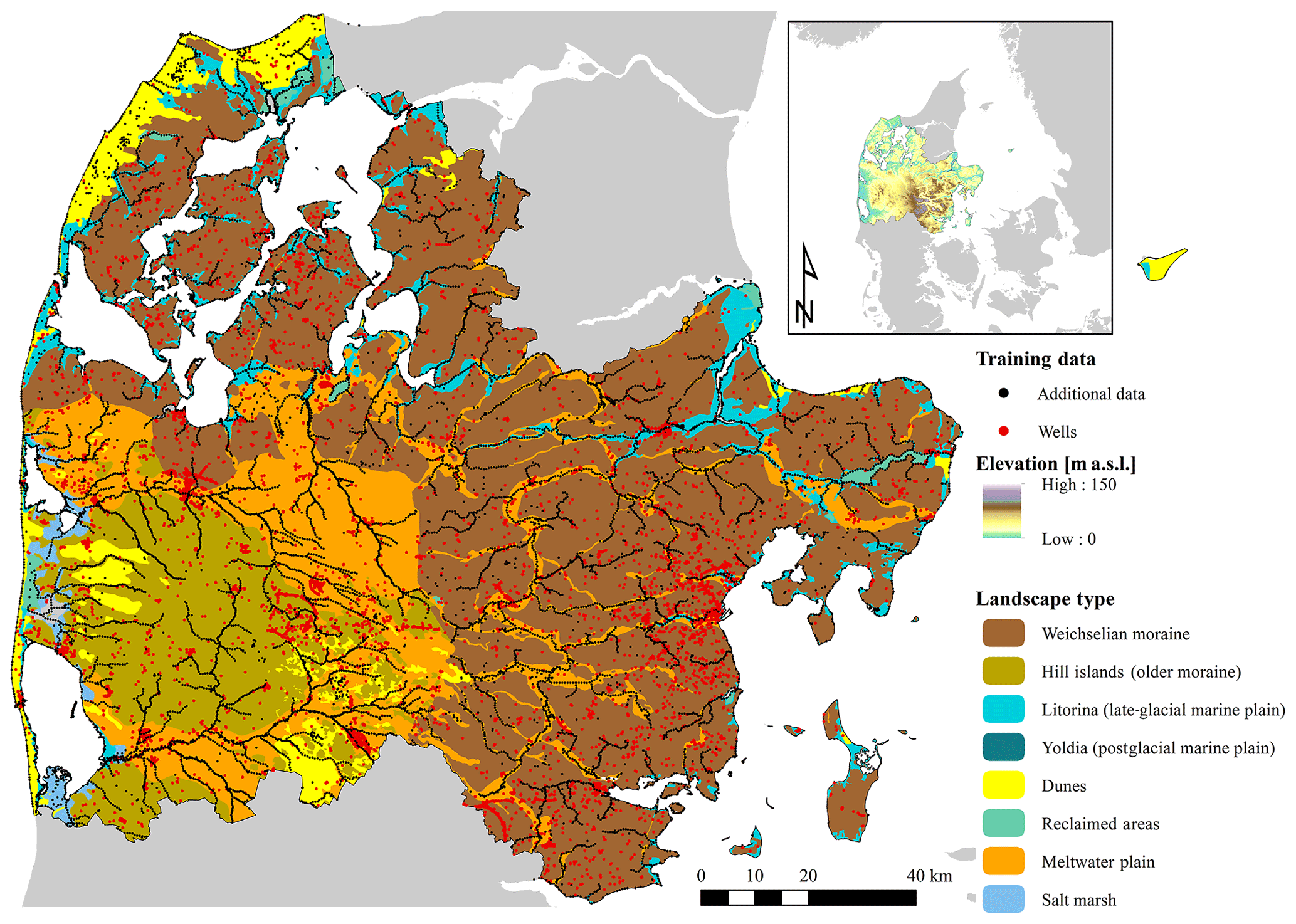
Figure 1 The study site is located in central Denmark. The inset figure is an overview depicting the digital elevation model. The main map shows the predominant geological landscape types. The training dataset contains observations at ∼15 000 wells. Additionally, ∼16 000 artificial observations, placed along major rivers, lakes and the coastline, are added to the analysis. The depth to the shallow groundwater is set to zero for the additional data.

2.2 Data

This study aims at modelling the depth to the shallow water table at a 50 m spatial resolution using a machine learning modelling framework. Disregarding the prevailing temporal variability of groundwater dynamics close to the surface, we chose to model an extreme event that characterizes a minimum depth which is expected to arise every year. Based on the climate in Denmark, such an event normally occurs towards the end of winter, when shallow aquifer systems are replenished after several months of typically high rainfall and low evapotranspiration. Applying machine learning to model an extreme event of a highly dynamic variable poses distinct challenges to the training dataset. Long time series of groundwater head measurements are scarce, and shallow groundwater time series are even more rare. In fact, many shallow wells, with screens within the uppermost 10 m, provide just one to a few observations in total. In order to capitalize on these low-frequency sampled wells, we developed a method to transform any given observations to an expected high water table. For this transformation, sinus curves were defined with varying amplitudes that captured the annual dynamics of the shallow groundwater for various hydrogeological settings. The workflow is described in more detail below.

First, well data, covering the entire model domain, were extracted from the national database, Jupiter (Hansen and Pjetursson, 2011). Groundwater head observations from wells with a maximum filter depth of 10 m were assorted for a 20-year period between 1998 and 2017. Several constraints were applied to this initial extraction: (1) the mean water level may not be below the filter depth, (2) the water levels may not exceed 5 m above the surface, (3) the standard deviation of the head observations may not be greater than 3 m and (4) the well may not be in operation. By applying these four constraints, 14 916 wells with one or more head observations were selected which approximately corresponds to a density of one well per square kilometre. Figure 1 shows the location of the wells.

Second, wells with more than five observations, of which 392 were present, were grouped according to their hydrogeological setting. Subsequently, their standard deviation was studied in more detail in order to define the sinus curve amplitudes for each of the groups. In total, 27 combinations, describing the general hydrogeological setting of a well, were assessed. These groups were based on three categories with three subcategories each, (1) permeability (high, low or unknown), (2) aquifer condition (confined, unconfined or unknown) and (3) proximity (near the coastline, near stream or other). The amplitude of the sinus curve was set to the 99 % confidence interval and, under the assumption of normality, calculated as 2.576 times the standard deviation. Based on the analysis of the variability at 392 wells with long time series the average annual amplitude of the sinus curves varied between 0.5 and 1.5 m depending on the hydrogeological setting. The largest amplitude was associated with wells with filters in sediment with low permeability, under unconfined conditions and not in the vicinity of the coastline or streams. Low amplitudes were generally connected with wells closer than 100 m to streams, lakes or the coastline. The minimum and maximum of the sinus curves was set to arise in mid-February and mid-August respectively.

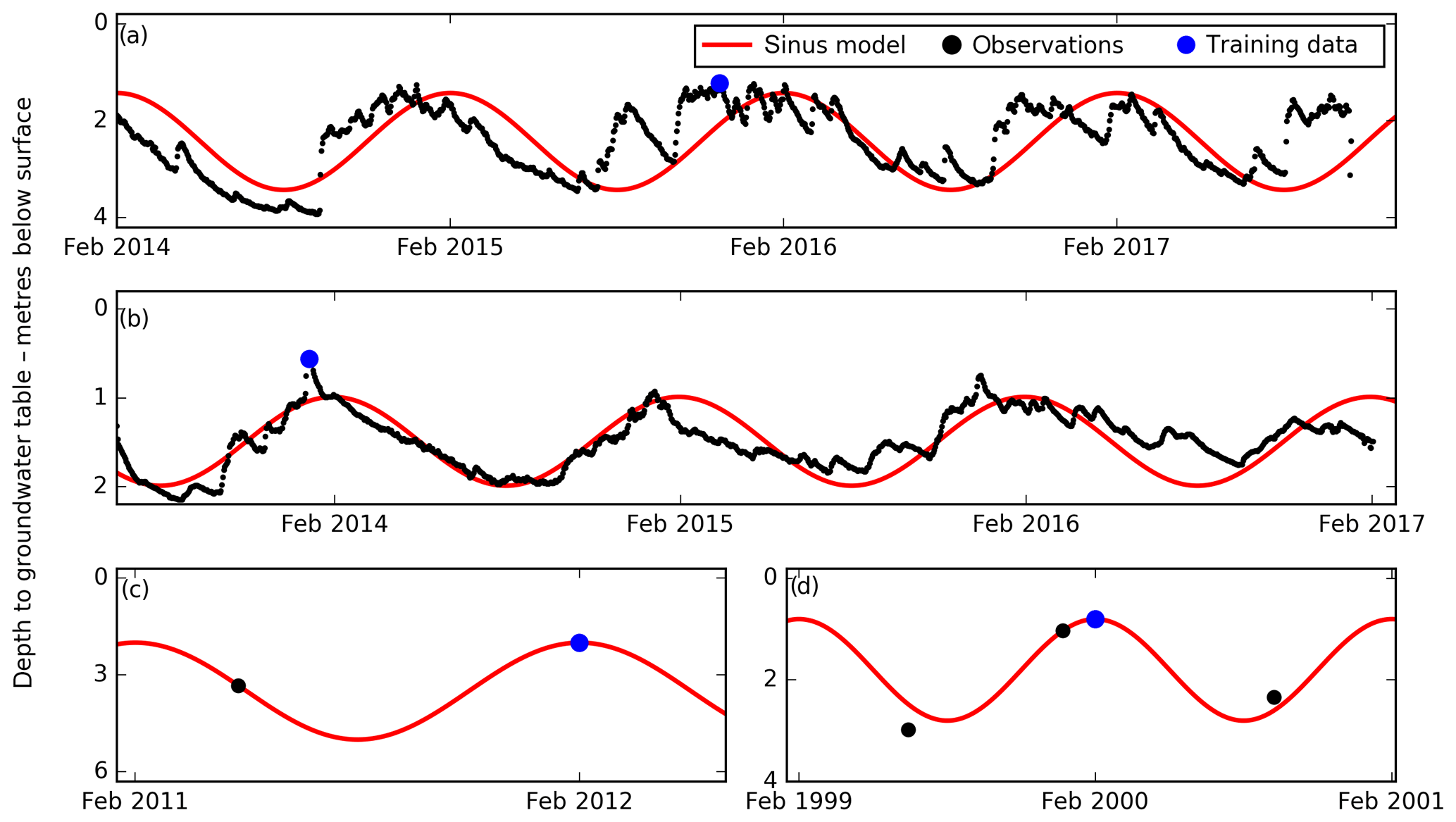
Figure 2 Four examples showing how the training dataset was derived. At wells with more than four observations (a, b), the minimum daily observation was chosen. Examples (a) and (b) represent long time series and sinus curves with amplitudes of 1 and 0.5 m respectively, and were used to describe the annual variability. Examples (c) and (d) represent two cases with few observations. Here, sinus curves with predefined amplitudes, 1.5 and 1 m respectively, corresponding to the well's hydrogeological setting were applied to traverse the observed minimum depth to an expected wintertime minimum.

Third, the groundwater head value describing an extreme wintertime condition at each well was defined twofold. At wells with five or more observations, the recorded minimum depth was used as input to the training dataset. Conversely, at wells with fewer observations, the predefined sinus model was applied to transform an observed minimum to an expected wintertime minimum. Using this approach, the observed variability at wells with high-quality data was used to infer a meaningful minimum value, describing an extreme wintertime situation, at wells with few observations. Figure 2 exemplifies this approach in more detail. The first two examples express wells with long time series, used to define the sinus amplitude corresponding to the well's hydrogeological setting. Here, the minimum observations were extracted as input to the training dataset. The bottom two examples depict cases with few observations where a sinus curve was applied to transform the observed minimum depth to an expected winter minimum condition. In cases where the transformation resulted in negative values, i.e. manifesting artesian conditions, the value was set to zero. This correction was considered meaningful as many of these wells were located in unconfined conditions. The resulting training dataset consisted of 14 916 wells; from these wells, 97 % were corrected with sinus curves, and the observed minimum depth was used at the remaining 3 %. Figure 2 indicates that the minimum depths based on the measured values and sinus model may deviate for the 392 wells with long time series. However, the two examples in Fig. 2 imply a deviation of 10–20 cm, which lies within the measurement uncertainty itself. This allows us to conclude that the proposed sinus model-based correction is robust enough for our application.

There are two sources of uncertainty that were not considered in this analysis. First, the observational uncertainty related to the head values in the well database was not taken into account. Second, the sinus model used to traverse any given observation to an expected wintertime minimum neglected seasonal and inter-annual variability.

Table 1 Overview of the covariates used to model the shallow water table using RF.

Additional observations were placed along streams, the coastline and the centre points of lakes. At the given locations, the depth to the shallow groundwater was set to zero. This extension of the training dataset was found necessary in order to provide critical information to the machine learning model which was otherwise not conveyed in the borehole data alone. However, only a subset consisting of 1900 random samples of the 16 210 additional observations was used for training of the machine learning model. This corresponds to approximately the same well density as found in the original training dataset, taking the combined area of streams, the coastline and lakes in 50 m grid resolution into consideration. In this way, the information content of the well data and the additional data was balanced. Including all ∼16 000 additional observations with a depth of zero in the training dataset would result in a biased model, because the average of the training dataset would not be representative for the study site. The complete dataset of additional observations was, however, utilized in the uncertainty analysis. In Table 1, a list of the environmental covariates used to model the depth of the shallow water table is found. In total, 27 covariates were assembled as input to the machine learning model. This list comprises information on soil texture, drainage conditions, geology, topography-based characteristics, water body proximity, precipitation, land cover, geographic location and outputs from a hydrological simulation with the Danish national water resources model (DK-model; Højberg et al., 2013). The native spatial resolution of the covariates varied, but all covariates were resampled to 50 m to be in agreement with the defined output resolution. The water body proximity was expressed as both the vertical and horizontal distance to the nearest water body, which contained rivers, lakes and the coastline. The covariates were subdivided into six groups, i.e. geology, topography, water body relation, precipitation, land cover, coordinates and hydrological model. This subdivision was implemented in the sensitivity analysis of the machine learning model to eliminate correlations between covariates.

2.3 Random forests

This study applied random forests (RF) regression to model the depth to the shallow water table at high spatial resolution at the regional scale. RF was first proposed by Breiman (2001) and has emerged as a prevalent modelling tool covering a wide range of geophysical and environmental contexts. These include, among others, digital soil mapping (Hengl et al., 2015; Ließ et al., 2012), estimating nitrate pollution in aquifers (Rodriguez-Galiano et al., 2014; Tesoriero et al., 2017), biomass estimation using satellite remote sensing (Mutanga et al., 2012), landslide susceptibility analysis (Youssef et al., 2016), mineral prospectivity mapping (Rodriguez-Galiano et al., 2015) or estimation of young water fractions across catchments (Lutz et al., 2018). RF has proven to provide high predictability for multivariate modelling of complex, non-linear variables, and multiple benchmarking studies have documented the capabilities of RF to outperform other machine learning techniques (Nussbaum et al., 2018; Rodriguez-Galiano et al., 2015; Youssef et al., 2016). Like other data-driven modelling approaches, training is an essential step in the RF model-building process. Based on the training dataset, RF learns linkages between the covariates and the target variable at sampled locations, which then are generalized to make predictions at unsampled locations. The core of RF is an enhanced utilization of decision trees. More precisely, RF builds an ensemble of decision trees, where each tree recursively splits the training data into more homogenous groups. The formulation of the decision trees contains two elements of randomness with the aim to increase the diversity within the ensemble of decision trees. First, the concept of “bagging” is applied. Bagging is an ensemble technique that generates a unique bootstrap sample of the original training dataset for each decision tree. Based on sampling with replacement, each bootstrap sample contains approximately 63.2 % of the original training data. The average across the entire ensemble represents the final RF prediction. Second, only a subset of the covariates is drawn upon when splitting the data during the process of decision tree building. This subset, usually 33 % of the available covariates, is selected randomly for each split. In combination, the two elements of randomness decrease the accuracy of a single tree; however, the diversity between the trees increases, which results in a robust prediction when averaging across all trees.

The bootstrapping procedure divides the training data into an “in-bag” part, which is used for building the decision trees, and an “out-of-bag” (oob) part, which is excluded from the training. This partitioning is unique for each tree of the ensemble and thereby provides a valuable internal cross-validation test. In other terms, each tree can be evaluated with its own oob sample, and the average across all oob predictions allows for the quantification of the overall accuracy of the RF model. For the oob prediction, only samples retained from the training, thus out-of-bag samples, are considered when averaging. In this way, the entire ensemble of trees can be evaluated by applying the oob approach. In order to quantify the performance of the RF model, we have applied the following metrics on the oob prediction: coefficient of determination (R²), mean absolute error (MAE) and root-mean-squared error (RMSE). We applied the Scikit-learn Python package (Pedregosa et al., 2012) to conduct the RF modelling for this study.

2.4 Covariate sensitivity

The concept of covariate permutation allows one to assess the importance of each covariate that acts as input to a RF model (Biau and Scornet, 2016). This can be understood as a sensitivity analysis which can help to better comprehend and interpret the trained RF model and to gain physical insights into the otherwise nontransparent black-box model. This is achieved by permuting each covariate at a time, while leaving the remaining covariates unchanged, and tracing the apparent decrease in the oob evaluation metric. Typically, the coefficient of determination (R²) is used as a metric, but other metrics could also be consulted as the sensitivity may be metric dependent. This concept is common practice to assess covariate importance for a trained RF model (Ließ et al., 2012; Lutz et al., 2018). However, this analysis is limited to the training dataset, and conclusions on which covariates dominate the prediction and how this varies spatially cannot be drawn. In order to gain insights into the spatial patterns of covariates' importance, we have developed a novel method, which applies the above-mentioned concept of covariate permutation on the prediction dataset instead of the training dataset. The aim of the sensitivity analysis is to identify a relative ranking of covariate importance for each simulation grid, which can ultimately provide increased interpretability. The starting point of the analysis is the trained RF model and its prediction at all simulation grids. Sequentially, each covariate is permuted, while leaving the remaining covariates unchanged, and the trained RF model is used to make a modified prediction. The difference between the modified and original prediction is recorded. The cycle of permutation and prediction is repeated n times until the mean difference across n permutations converges for each simulation grid. This is necessary, because a single permutation may allegedly result in no or minor change in a covariate value at specific grids. Once the mean difference has converged, the covariates can be ranked with respect to their associated mean absolute difference for each simulation grid. In order to map the spatial covariate sensitivity it is essential that the ranking is performed at each simulation grid. This ranking expresses the relative covariate importance and is the key result of the proposed sensitivity analysis. Maps showing the top ranks can be used to visualize the spatial patterns of the sensitivity of the RF model.

Typically, strong correlations are found between covariates, which may result in an alleged low importance when being permuted individually (Koch et al., 2019). In order to overcome this limitation, we suggest a supplementary analysis that collectively permutes groups of covariates that are physically related.

2.5 Random forests regression kriging

Extending RF using geostatistical methods is gaining popularity in the field of digital soil mapping (Guo et al., 2015; Hengl et al., 2015) and related environmental modelling studies (Ahmed et al., 2017; Li et al., 2011; Viscarra Rossel et al., 2014). Regression kriging (RK) is a widely applied approach that combines a multiple linear regression (MLR) model with a geostatistical model of the MLR residuals (Hengl et al., 2007; Odeh et al., 1995). In order to integrate RF into RK, RF can simply replace the MLR model. In this way, RF provides an overall data-driven trend and the RF residuals can be interpolated using geostatistics. This results in a hybrid model that is commonly referred to as random forests regression kriging (RFRK). To our knowledge, RFRK has not yet been applied with the purpose of predicting a hydrological state variable such as groundwater head. RFRK can be expressed by

$$\begin{array}{}\text{(1)}& P_{\mathrm{RFRK}}\left(s_{\mathrm{0}}\right)=T_{\mathrm{RF}}\left(s_{\mathrm{0}}\right)+{\widehat{e}}_{\mathrm{RF}}\left(s_{\mathrm{0}}\right),\end{array}$$

where T_RF(s₀) is the RF prediction at location s₀ and ${\widehat{e}}_{\mathrm{RF}}\left(s_{\mathrm{0}}\right)$ is the estimated residual at the same location. The sum of trend (T_RF) and residual (${\widehat{e}}_{\mathrm{RF}}$) yields the final RFRK prediction (P_RFRK). This study utilizes kriging to interpolate the oob residuals of the RF model. We use the oob prediction instead of the overall RF prediction to compute the residuals, because the oob procedure provides a more realistic estimation of the generalization error. The overall RF prediction naturally exhibits a lower error than the oob predictions as the data were contained in the training. Therefore, the resulting error variance would be biased and can not be used to interpolate the error at unsampled locations. Kriging is a popular geostatistical technique for spatial interpolation that employs knowledge about the spatial autocorrelation of a variable, which can be captured by a variogram model. For the definition of a variogram model, the omnidirectional empirical semivariance (γ) is calculated by

$$\begin{array}{}\text{(2)}& \mathit{\gamma }\left(h\right)={\displaystyle \frac{\mathrm{1}}{\mathrm{2}n\left(h\right)}}\sum _{i=\mathrm{1}}^{n\left(h\right)}{\left[e\left(s_i\right)-e\left(s_i+h\right)\right]}^{\mathrm{2}},\end{array}$$

where n(h) marks the total number of data pairs at a given lag distance h, e(s_i) represents the oob residual at location s_i and e(s_i+h) is the residual separated by lag h from s_i (Matheron, 1963). A variogram model is fitted to γ to model the spatial autocorrelation structure of the oob residuals (Clayton and Andre, 1998). The parameters defining a variogram model are type, range, sill and nugget. The Gstat R package (Pebesma, 2004) was applied for variogram modelling and kriging interpolation.

The addition of residual kriging to RF results in high accuracy at grids coinciding with observations. Furthermore, kriging quantifies the prediction uncertainty following the defined variogram model. Generally, the kriging variance is low in the vicinity of data points and increases to the sill value once the distance to the nearest data point is beyond the range of the variogram model.

2.6 Quantile regression forests

Using RF, the prediction is obtained by averaging across the ensemble of decisions trees. This disregards the distribution of the target variable originating from several hundreds to thousands of decision trees, which are typically necessary to build a robust RF model. Meinshausen (2006) developed the quantile regression forests (QRF) method that analyses the quantiles of the distribution of the target variable at prediction grids. This results in an estimation of prediction uncertainty or prediction intervals. The latter is obtained by recording specific quantiles which mark the lower and upper confidence limits (Hengl et al., 2018). The adoption of QRF for hydrological variables is still gradual and only a few studies have documented its applicability (Francke et al., 2008; Zimmermann et al., 2014). To our knowledge QRF has not been applied to quantify uncertainty of groundwater level predictions. For this study, we utilized the RF functionalities from Scikit-learn (Pedregosa et al., 2012) to implement QRF.

3 Results

3.1 Random forests model

For the purpose of modelling the depth to the shallow water table at a 50 m spatial resolution for an extreme wintertime minimum event, a RF model was trained using the 27 available covariates and groundwater head data. The training data comprised ∼15 000 wells and 1900 additional observations placed along streams, the coastline and in lakes. After initial testing, the RF model was parameterized as follows: the number of decision trees was set to 1000, bootstrapping with replacement was applied to sample the training data, 33 % of the covariates were considered to identify the optimal data split, trees were fully expanded (and thus not pruned), the mean squared error was selected as criterion to identify the optimal data split and regression was chosen as the modelling method.

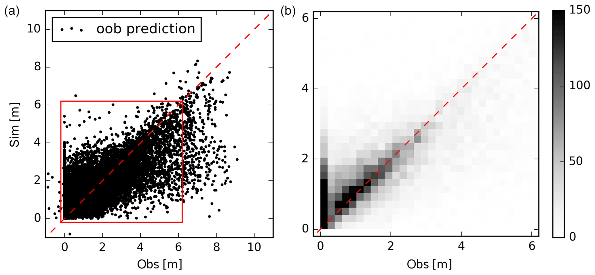
Figure 3 The RF accuracy assessment was performed based on the out-of-bag sample technique. The axes depict the simulated (Sim) and observed (Obs) depth to the shallow water table. Panel (a) displays a standard scatter plot containing ∼15 000 well data points. The 1900 additional observations are excluded. Panel (b) shows a zoom-in (extent indicators in red in panel a) and the data are visualized as a density scatter plot. The colour bar represents the number of data points in each square.

Figure 3 depicts the internal cross-validation test based on the oob samples of the well data. The oob prediction can be considered as an independent evaluation test, and the three performance metrics, i.e. coefficient of determination (R²), mean absolute error (MAE) and root-mean-squared error (RMSE), indicated an overall good performance (Table 2). More than half of the variance contained in the training data was captured by the RF model, the MAE amounted to 76 cm and the RMSE was 1.13 m. The density scatter plot in Fig. 3 zooms into the top 6 m, and it becomes apparent that very shallow observations (<0.5 m) were systematically biased while deeper observations were estimated in good agreement (close to the 1 : 1 line).

Table 2 Comparison of the RF generalization error quantified by the out-of-bag (oob) procedure and 10-fold cross-validation (cv) based on three metrics, i.e. coefficient of determination (R²) root-mean-squared error (RMSE) and mean absolute error (MAE). The 1900 additional observations were excluded for this evaluation.

In order to investigate if the oob prediction is a reliable source to quantify how generalizable a RF model is, we conducted a 10-fold cross-validation (cv) test. For this test, the dataset was randomly split into 10 sets of approximately the same size. Then 10 RF models were trained on 90 % of the data so that each set was left out once and could be used for evaluation purposes. The cv results were strikingly similar to the oob prediction (Table 2). The agreement was convincing which qualified the oob prediction as an appropriate way to quantify the generalization error of our RF model.

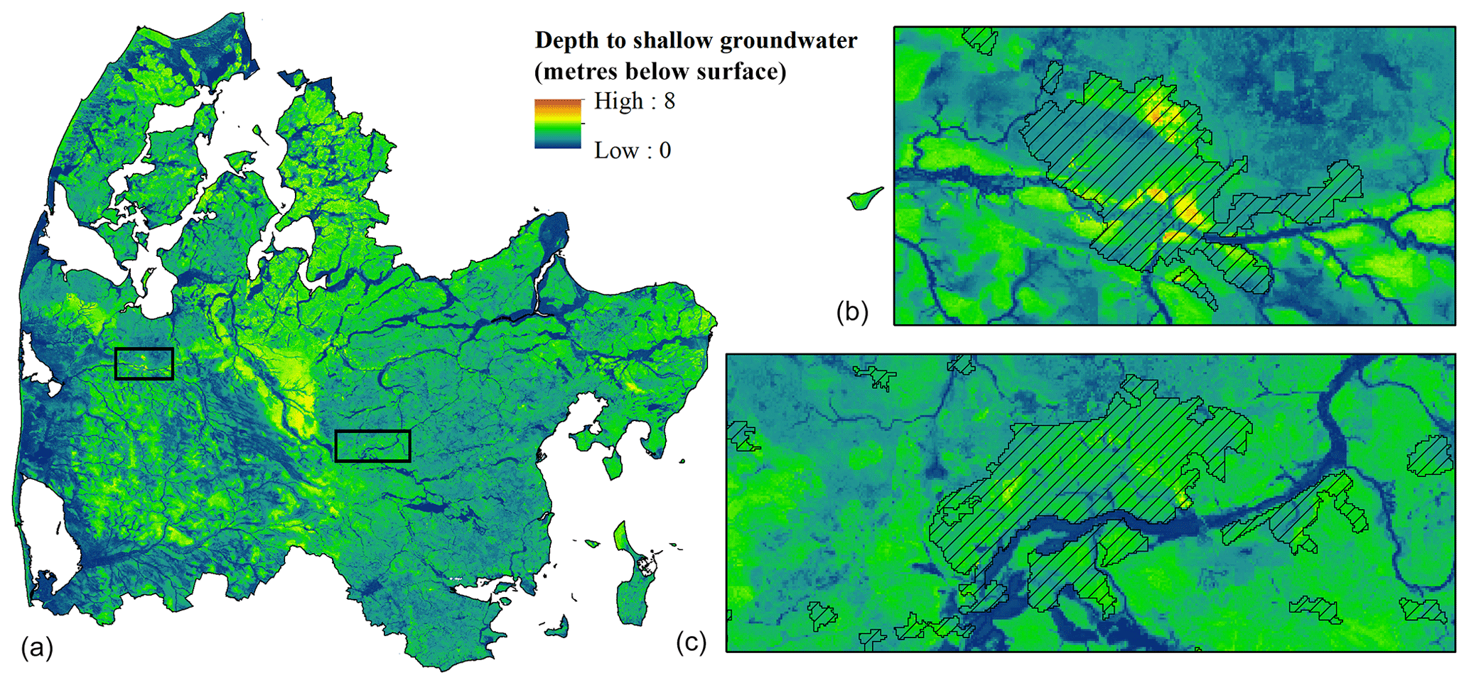
Figure 4 The resulting map of the depth to the shallow water table at a 50 m grid resolution. The zoomed-in extents highlight two urban areas. Panel (b) displays the city of Holstebro, and panel (c) depicts the city of Silkeborg. Urban areas are visualized using hatching.

Post training, the RF model was utilized to predict the depth to the shallow water table and the resulting map is shown in Fig. 4. Regional patterns of the shallow water table were estimated as expected with deeper water tables in parts of the sandy meltwater plains in the western section of the domain and a water table that was generally close to the surface in the moraine landscape, as shown in Fig. 1. Areas with low topography were usually exposed to a very shallow water table, which also corresponded to the conceptual understanding of the system. The 50 m spatial resolution provided a very detailed picture of the spatial patterns associated with the water table and the complex interplay of the covariates became apparent. This is shown on the basis of two zoomed-in extents, highlighting urban areas, in Fig. 4. The stream network and lakes are clearly visible with a depth of zero, which indicates that appending the additional observations to the training data resulted in the intended effect. The severity of the risk of groundwater-induced flood events becomes apparent through the statistics of the RF map. The mean depth to the groundwater for a typical wintertime minimum event constituted 1.9 m for the entire modelling domain. Around 29 % of the domain was characterized by a depth to the shallow groundwater of less than 1 m and a depth of 50 cm or less for 14 % of the area.

3.2 Covariate sensitivity

Covariate sensitivity was analysed from two different perspectives, both using the concept of permutation accuracy. First, sensitivity was assessed for the trained RF model based on the decrease in the R² of the oob prediction as a consequence of permuting a covariate. For this, only the training dataset was incorporated which resulted in an overall covariate sensitivity score. Second, the sensitivity of the trained RF model was estimated individually for each simulation grid based on the absolute difference between the permuted prediction and the original prediction. This approach gives the relative ranking of the most sensitive covariates for each simulation grid. Figure 5 shows the results for the former. The vertical distance to the nearest water body was the dominant covariate for the simulation of the shallow water table. A decrease of 60 % in performance was apparent when the variable was permuted. We found a direct relationship between the two variables, which highlighted that the shallow groundwater did not explicitly follow terrain variability. This resulted in a relatively deep water table at locations where the vertical distance is high and vice versa. The second-most important variable in the trained RF model was the simulated water table by the national water resources model (DK-model), associated with a 15 % drop in performance when being permuted. The DK-model provides a typical minimum depth to the shallow water table at a 500 m resolution for a 20-year reference period (1991–2010). This indicated that the DK-model could supply a valuable coarse trend to the RF model.

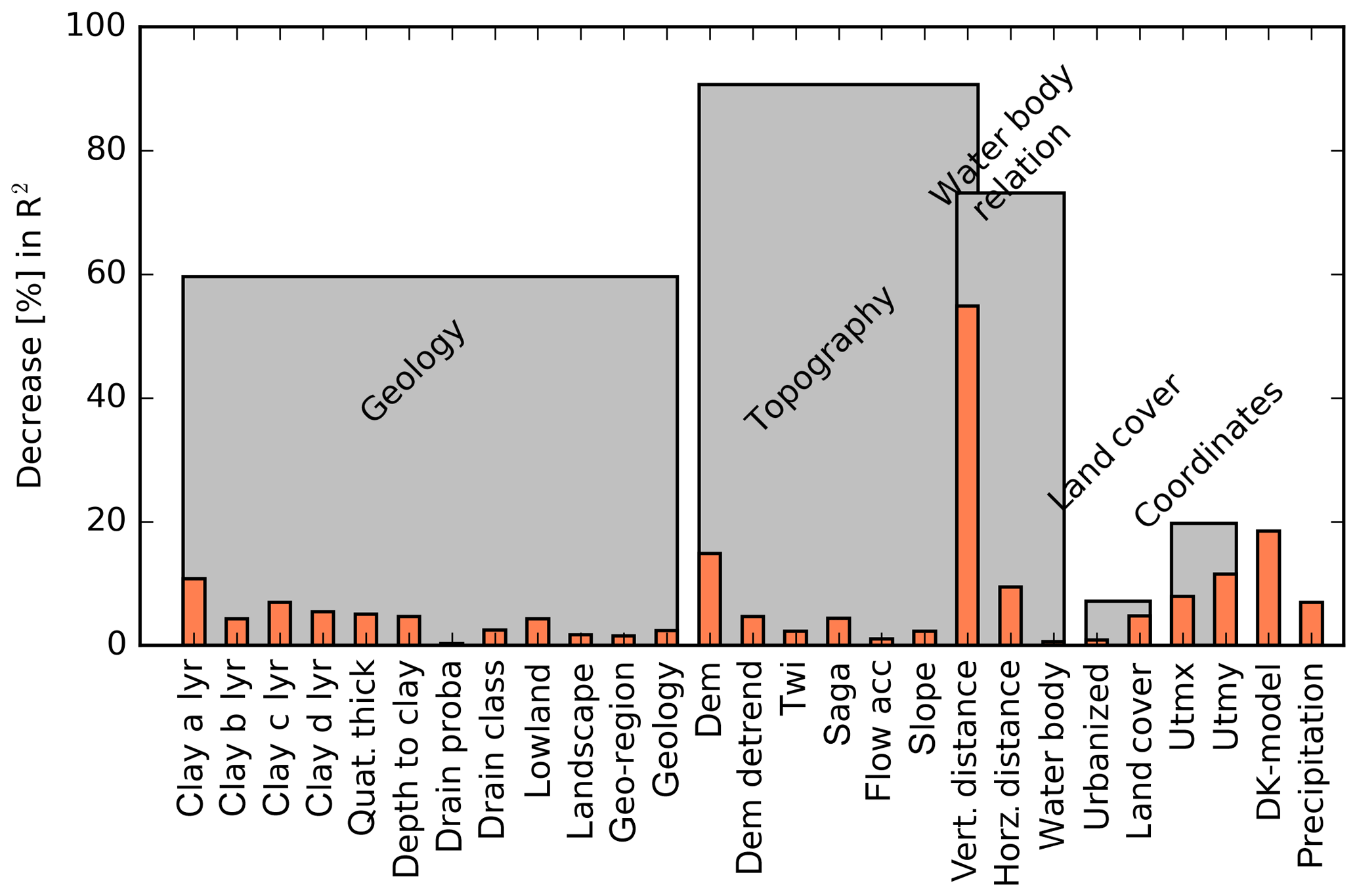
Figure 5 Variable importance of the trained RF model. The concept of permutation accuracy was implemented to quantify the decrease in out-of-bag performance R². Permutation was applied not only to single covariates (orange) but also to groups of covariates (grey). Covariates are further specified in Table 1.

Figure 5 also quantifies the importance of physically related covariates. When permuted collectively, covariates associated with the topography resulted in a decrease of nearly 100 % in performance; thus, the respective covariates formed the most important group. They were followed by covariates describing the water body relation (∼70 % drop in performance) and geology-related variables (60 %). As the vertical distance to the nearest water body relates to both, topography and water body proximity, it was included in both groups. The above-mentioned results are based on the relative decrease in the R² caused by the permutation of the covariates. In order to test if the resulting sensitivity ranking is metric dependent, we conducted the same analysis based on the relative decrease in the RMSE. We concluded that, in spite of varying absolute numbers, the same conclusion in terms of relative covariate sensitivity could be drawn; therefore, the results are not discussed further in this study.

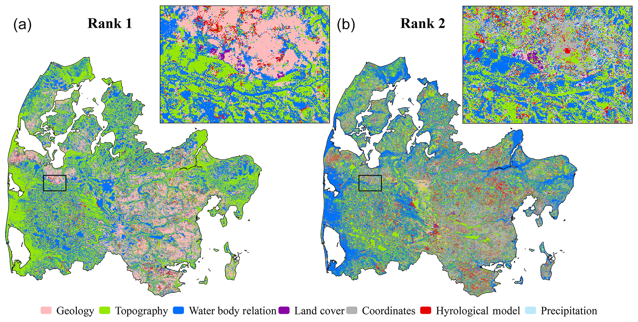
Figure 6 The results of the sensitivity analysis are shown for the most sensitive covariate group (Rank 1, a) and the second-most important covariate group (Rank 2, b). The city of Holstebro is chosen as the zoomed-in region for both maps.

The results from the spatial sensitivity analyses are presented in Fig. 6. Figure 6 depicts maps of the top two most important covariates for the RF prediction. Covariates were permuted collectively following the groups presented in Table 1 and as applied in the sensitivity analysis of the trained RF model (Fig. 5). Each covariate group was permuted 250 times to ensure that the difference to the original RF prediction converged at the individual grids. The simulated water table in the moraine landscape in the eastern part of the model domain was controlled by covariates related to the geology. Here topography is gently undulating and sediments are clay rich, which, in combination, resulted in a water table close to the surface with small-scale variability caused by geological heterogeneity. The second-most important covariates in the moraine landscape were mainly the DK-model or the UTM coordinates. This underlined the complexity of the shallow water table in this landscape. The DK-model includes a comprehensive analysis of the entire system, taking the interplay between several factors (hydrogeology, topography, climate and others) into consideration. In the RF model, coordinates provided the only possibility to assign uniqueness to a simulation grid, which was required in the moraine landscape to capture the complexity of the shallow water table. Topography was important at locations close to sea level or areas that were generally plane. Water body relations played an important role at locations that were either very far away from or very close to a water body. Data on the location of urban areas, which were contained in the land cover group, were rated important for urban areas with moraine soils. In such clayey conditions, the subsurface is often drained resulting in a deeper water table. Overall, the importance of the DK-model appeared to be very local and generally scattered across the domain, which underlined the relevance of this covariate, as it could provide coarse information at locations where the standard covariates fail to provide a meaningful generalization.

3.3 Uncertainty analysis

For the uncertainty analysis, we employed two methods, namely RFRK and QRF. For the first, the RF residuals were interpolated using kriging. Figure 7 shows the variogram model which was used in the kriging interpolation. The nugget was set to 0.26 m² and the sill was defined as 1.02 m². An exponential variogram with a range of 700 m gave the most satisfying fit to the experimental semivariances calculated at a 200 m lag distance.

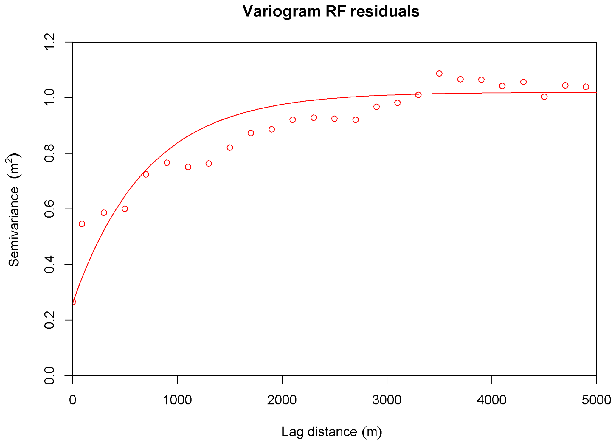
Figure 7 The computed semivariances for the RF residuals (circles), based on the oob prediction. The line expresses the fitted variogram model.

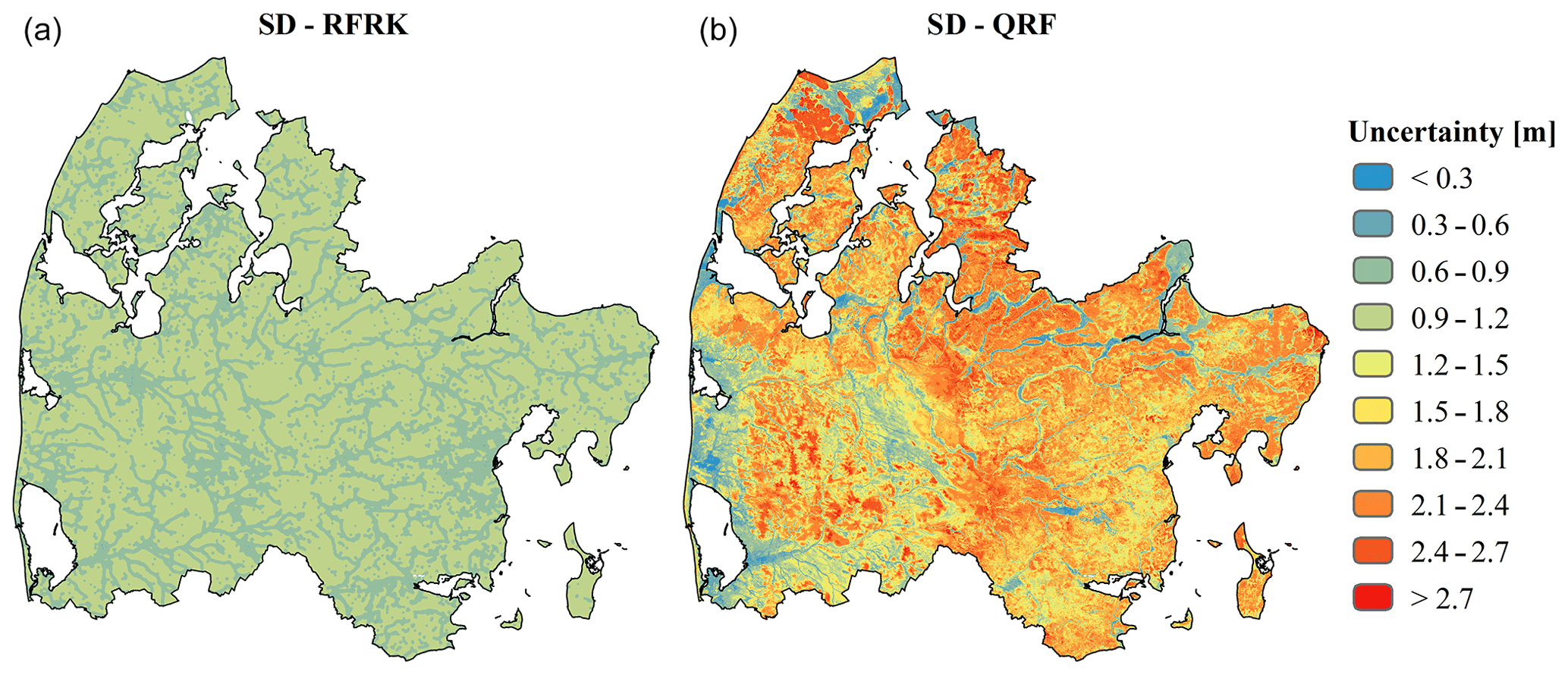
Figure 8 Two methods to quantify the uncertainty of a RF model are implemented: RFRK (a) and QRF (b). For all maps, uncertainty is expressed as the standard deviation (SD).

Figure 8 depicts the resulting uncertainty, which was expressed by the standard deviation for both of the methods applied. The RFRK employed all available data, ∼15 000 wells and ∼16 000 additional observations along streams, the coastline and in lakes, in the RF residual interpolation. Conversely, the RF training dataset only contained 1900 additional observations in order to have a balanced relationship between well data and additional observations in terms of data density. Following the predefined variogram, uncertainty was low in the vicinity of an observation, which increased with distance until the sill value was reached. In this way, all grid cells with a distance to a well or an additional observation larger than the correlation length of the variogram model exhibit no variation. Based on QRF, the derived uncertainty shows a different picture. Here the uncertainty was expressed as the standard deviation of the 1000 individual decision tree predictions at each grid cell. In general the uncertainty estimated by RFRK was lower than QRF. In the western section, high uncertainties were generally associated with locations with a large depth to the shallow groundwater and vice versa for the QRF-based assessment. However, the moraine landscape in the eastern part was characterized by an overall high uncertainty despite having an overall water table that is close to the surface. Such physical dependencies that relate to the structure of the RF model were not captured by the RFRK approach, which purely reflected borehole proximity. The mean uncertainty across the domain amounted to 0.92 m for RFRK and 1.68 m for QRF.

4 Discussion

4.1 Training dataset

In order to capitalize on undersampled wells, this study utilized sinus curves with amplitudes fitted to observations at wells with long time series according to their hydrogeological setting. Even though this step introduced uncertainties, it was essential to generate a training dataset large enough to make robust predictions. Applying the same amplitude every year did not distinguish between dry and wet years, which was a clear limitation of the approach. The sinus curves described an average seasonal variation within a hydrogeological class of boreholes and were thus not designed to reflect the variability of all boreholes within each class. Nevertheless, it was critical that the dataset used to train a RF model contained a wide range of observations before the model was able to generalize and make predictions. Along these lines, a training dataset can be expanded based on expert domain knowledge to capture otherwise underrepresented conditions (Koch et al., 2019). In this study, additional observations along streams, the coastline and in lakes were appended to the training dataset with a depth to the water table of zero. In regions where the connection between surface and groundwater is generally good, like it is for this case in Denmark, the extent of surface waters can be considered a reliable proxy of the shallow water table. The additional observations used in this study guided the RF model to produce more reliable predictions. Initial tests without the additional observations resulted in surface water bodies which were unconnected to the shallow groundwater system.

In unconfined sandy aquifers, we assume the elevation of the shallow water table to be more homogeneous than the depth of the shallow water table. This assumption may not apply for more complex geological settings, such as glacial tills, which cover a majority of the study area, where a secondary water table often follows the surface elevation. This motivated us to model the water table depth instead of the elevation, which was further supported by an initial test where a RF model was trained to predict the water table elevation. The resulting water table elevation could easily be converted to depth via subtraction from the surface elevation, and results indicated poorer performance compared with the RF model predicting the water table depth.

The RF model was trained to a single event and thus disregards the temporal dynamics of the shallow groundwater system. As the model was designed as a simple screening tool, this can be considered an advantage; however, much of the complexity is not considered which is a clear shortcoming of the proposed method.

In the coming years, the Danish national water resources model (DK-model) will be updated based on recent hydrogeological interpretations and reconstructed at a 100 m spatial resolution. This is expected to improve the predictability of the shallow water table, and the DK-model output should then be utilized to update the RF model.

4.2 Random forests model

This study utilized the oob prediction to validate the performance of the RF model based on three metrics, namely the coefficient of determination (R²), mean absolute error (MAE) and root-mean-squared error (RMSE). The metric scores were very satisfying overall and in the range of what could be considered very acceptable in groundwater flow modelling (Henriksen et al., 2003). These findings underpin the applicability of RF to model complex, non-linear variables with an accuracy that is difficult to obtain with physically based models. In contrast, the accuracy assessment revealed a systematic bias of the trained RF model that was affecting wells with groundwater levels close to the terrain. The biased wells were predominately located in clayey moraine sediments, which indicated location-specific shortcomings of the RF model. The geology of the moraine landscape is heterogeneous which impacts the hydrogeological setting and, in turn, also the shallow groundwater (He et al., 2014, 2015). At the current stage, the available national hydrogeological data do not possess the required spatial resolution to resolve the apparent heterogeneities adequately. Moreover, some of the above-mentioned wells are placed in confined conditions, which in combination with the heterogeneous geology may hinder good performance of the RF model.

Studying the covariate importance identified the water table simulated with the DK-model at a 500 m resolution as the second-most important RF input. These results were very promising as the applied RF framework forms a straightforward implementation of unifying machine learning and physically based models. More precisely, RF built upon the coarse DK-model using high-resolution covariate information that ensured physical consistency.

Some covariates, e.g. drainage characteristics and the topographic wetness index, were assigned an unanticipated low importance in the sensitivity analysis of the RF model (Fig. 5). This may indicate covariate redundancy or the fact that the metric to quantify covariate importance (the decrease in the coefficient of determination) is not very sensitive to the permutations that may result in changes in wells with a very shallow water table. For comparison, the RMSE instead of the R² was applied to quantify covariate importance, but this test did not provide any additional insights. Future work must systematically address the issues related to the choice of metric or the fact that certain parts of the distribution are more sensitive to different covariates.

The resulting spatial resolution of 50 m provides a valuable screening tool for water management purposes. The risk of groundwater floods on agricultural fields or urban areas is typically very local and driven by small-scale variations of topography and geology. This makes high-resolution predictions inevitable in order to reliably tackle the related challenges. At the regional scale, the 50 m resolution would not be feasible with numerical modelling, which emphasizes the versatile applicability of RF. Many covariates are available at a finer resolution and, as computational power becomes more and more dispensable, RF predictions at even higher resolution are within reach. This development should also build upon current improvements of physically based models, which are now already capable of providing results at resolutions in the range of hundreds of metres (Ko et al., 2019; Wood et al., 2011) and, thus, such models could provide valuable trends, used as covariates in machine learning models.

This study proposed a novel approach to quantify the covariate sensitivity of the simulation dataset, which results in a relative ranking of the most important covariates at the grid level. This analysis provided physical insights into the driving mechanisms and, in general, the findings corresponded to the conceptual understanding of the hydrogeology in the study area. Such sensitivity maps are extremely valuable for both the modeller and the stakeholders working with RF predictions. The former group can validate the physical consistency of the otherwise nontransparent black-box model and the latter will have a better understanding and ultimately also a greater acceptance of the predictions.

4.3 Uncertainty assessment

This study assessed the capabilities of RFRK and QRF to estimate the uncertainties associated with a RF model that predicts water levels of the shallow groundwater system. Uncertainty was expressed by the standard deviation; alternatively, both methods could also be utilized to map upper and lower uncertainty bounds that represent certain confidence intervals. The key differences between the two proposed methods were as follows: (1) the uncertainty estimation of RFRK was generally lower than QRF and (2) the spatial patterns were diverging; RFRK only reflected borehole proximity, whereas QRF manifested a physical dependency of the uncertainty estimation. These findings are in line with recent comparison studies focusing on QRF and RFRK from the digital soil mapping literature (Szatmári and Pásztor, 2018; Vaysse and Lagacherie, 2017). Szatmári and Pásztor (2018) argue that RFRK-based uncertainty estimations are limited because results do not depend on the data value; therefore, the method expresses an unconditional variance. This stringent assumption of homoscedasticity, i.e. constant error variance, could be unrealistic for variables where the variance behaves proportionally to the measured value (Hengl et al., 2018). Moreover, RFRK assumes that the RF prediction, which is used as a trend, is certain; thus, the kriging variance only reflects the distance to the nearest observation. This assumption is too optimistic, as the uncertainty in the RF prediction is neglected. Once the training dataset is processed, RF disregards any uncertainties associated with the values of the target variable. In this study, uncertainties could originate from the applied sinus model used to transfer the observations to a typical wintertime minimum depth as well as the observations itself. In contrast, a physically based hydrological model allows more transparency, as biased observations will be marked as outliers in the model evaluation. However, a data-driven model, as flexible as RF, will incorporate such outliers – thus biased predictions may arise.

As stated by Vaysse and Lagacherie (2017), QRF quantifies information regarding where a simulation point is located in the covariate space. In this way, QRF properly discriminates groundwater conditions of contrasted physical complexities, of which some are better constrained by the training dataset than others. We argue that the RFRK shortcomings of assuming certainty in the trend prediction can be alleviated by the addition of QRF, which can capture the uncertainty of the RF model structure. In summary, RFRK captures uncertainty related to the geographical space, whereas QRF describes uncertainties related to the covariate space. More work is needed to integrate these two sources of uncertainty into a single uncertainty quantification.

Reducing uncertainties can be achieved by collecting more observations and, thus, expanding the training dataset. Especially in the eastern part of the domain, which is characterized by a high clay content and a heterogeneous surficial geology, additional data would likely reduce the uncertainty. A measuring campaign in wintertime, when the shallow groundwater system is fully replenished, would be very beneficial to advancing the modelling capabilities. Additionally, a higher spatial resolution may contribute to an uncertainty reduction, as observations can be represented more uniquely by the covariates.

In more general terms, as the numbers of hydrological applications based on machine learning are vastly expanding, standards on how to conduct uncertainty analyses must be formalized in the same fashion as was carried out for numerical modelling (Refsgaard et al., 2007). Ultimately, such a development determines the stakeholder acceptance of machine learning results.

5 Conclusions

This study focused on using RF to predict a map that depicts the depth to the shallow groundwater at a 50 m resolution for a typical wintertime minimum. More precisely, to predict a minimum event that is expected to occur annually and poses the risk of groundwater flooding affecting both urban areas and agricultural fields. The regional map will be extremely valuable for water resources management. We draw the following main conclusions from our work:

1. RF is a versatile modelling tool with high accuracy that enables spatial detail beyond the possibilities of (physically based) numerical modelling. The depth to the shallow water table was modelled with a mean absolute error of 76 cm for an independent evaluation test.

2. Predictions from a coarse physically based model that represent an overall trend of the water table can be utilized by RF as a covariate. In this way, RF ensures physical consistency at coarse scale and exhausts high-resolution information from topography, geology and other relevant variables. The DK-model at 500 m resolution was rated the second-most important covariate in the trained RF model, indicating that this simple form of unifying machine learning and physically based modelling has great potential.

3. The novel approach to assess covariate sensitivity for the prediction dataset goes beyond the standard applications where covariate importance is solely quantified for the training dataset. Results provide valuable insights on the spatial pattern of covariate sensitivity and can contribute to generating acceptability among end-users. The increased interpretability of the RF predictions can reassure modellers by comparing the derived sensitivity patterns with their conceptual understanding of the system.

4. In the general context of hydrological machine learning applications, more experience must be gained on how to properly quantify uncertainty. RFRK was found useful to assess observational proximity, but assuming certainty in the RF predications was regarded a shortcoming. This can be compensated for by QRF, which is capable of addressing the uncertainty related to the structure of the RF model. However, methods to remove the uncertainties related to the observations themselves and possible preprocessing of the training dataset are still lacking.