Statistical approaches for identification of low-flow drivers: temporal aspects

The characteristics of low-flow periods, especially regarding their low temporal dynamics, suggest that the dimensions of the metrics related to these periods may be easily related to their meteorological drivers using simplified statistical model approaches. In this study, linear statistical models based on multiple linear regressions (MLRs) are proposed. The study area chosen is the German federal state of Lower Saxony with 28 available gauges used for analysis. A number of regression approaches are evaluated. An approach using principal components of local meteorological indices as input appeared to show the best performance. In a second analysis it was assessed whether the formulated models may be eligible for application in climate change impact analysis. The models were therefore applied to a climate model ensemble based on the RCP8.5 scenario. Analyses in the baseline period revealed that some of the meteorological indices needed for model input could not be fully reproduced by the climate models. The predictions for the future show an overall increase in the lowest average 7-day flow (NM7Q), projected by the majority of ensemble members and for the majority of stations.

1 Introduction

Low flows appear ideal for the analysis of statistical dependencies with their meteorological drivers, due to their specific characteristics. As opposed to high flows, low streamflow is usually far less dynamic, and its meteorological drivers, i.e., primarily a lack of rain and increased evaporation, are observable over much larger scales in both time and space. Accordingly, several studies have aimed at explaining observed peculiarities in low flows by climatic phenomena, including Mosley (2000), who analyzed the influence of El Niño and La Niña effects on monthly lowest 7-day flow in New Zealand. He determined a major deviation of low flows from the normal in La Niña years. Haslinger et al. (2014) found that correlations between streamflow anomalies and meteorological drought indices are high, especially within the low-flow period. Van Loon and Laaha (2015) analyzed the dependence of streamflow drought duration and deficit volume on climatic indicators and catchment descriptors, while Liu et al. (2015) estimated the parameters of a GEV distribution fitted to the low-flow time series at their gauge in China as functions of a set of climatic indices.

Based on these findings it is hypothesized that streamflow metrics describing low-flow events may be efficiently assessed based on their relationship with metrics of meteorological states. This assumption entails that simple statistical models may be formulated that allow a reproduction of low-flow metrics based on meteorological input. In this study the relationship between annual low flow and a variety of meteorological indices will be analyzed with the aim of formulating simple statistical models. Such models will be set up individually for each catchment in the study area and are supposed to be capable of predicting low flow as a simple function of several relevant meteorological indices in time. Various temporal scales will be considered for the meteorological data and the most adequate ones for each catchment will be identified. The model fitting itself will be carried out using various statistical approaches in order to account for different effects, like non-stationarity or serial dependence in the annual low-flow indices. In order to assess the performance of the strictly linear statistical approaches, they will be compared to a hydrological model, which is assumed to accurately reproduce rainfall–runoff relationships by involving more complex processes, relying on continuous meteorological input. This analysis will reveal whether the statistical models fail to acknowledge important nonlinear relationships.

Apart from identifying relevant low-flow drivers, we test whether the use of the formulated statistical models may be extended to prediction of future low flows, using meteorological input from climate models. The probably most common approach in hydrological climate change impact analysis is to drive hydrological models, usually rainfall–runoff models of variable complexity, with regional climate model data input, obtained for various emission scenarios. Also for low flows this model chain has been applied for impact assessment in several studies, e.g., by de Wit et al. (2007), Schneider et al. (2013), Forzieri et al. (2014), Wanders and Van Lanen (2015), van Vliet et al. (2015), Roudier et al. (2016), or Gosling et al. (2017). The statistical models may pose an alternative simpler impact model approach that is easily set up and applied to large numbers of catchments and extensive climate model ensembles – while predicting hydrological quantities with sufficient accuracy. They may thus offer a different yet convenient tool for comprehensive regional climate change impact analyses. According to this hypothesis, the formulated models will be applied to an ensemble of regional climate model data in order to assess the plausibility of their low-flow projections in the future.

2 Study area and data

2.1 Study area

The area under investigation is the federal state of Lower Saxony situated in northwestern Germany. Its total area of 47 634 km² extends from the North Sea in the northwest to the Harz mountains in the southeast. The largest portion of Lower Saxony is part of the North German Plain, where the terrain is generally flat and low. The highest elevations are found in the secondary mountains of the Harz, at up to 971 m a.s.l. The topography is depicted in Fig. 1.

Figure 1 Study area with stations available for different analyses.

2.2 Base data

The meteorological data used in this work comprise daily time series of precipitation, temperature, and global radiation. The data are made available continuously in space via interpolation onto a 1×1 km raster for the total area of Lower Saxony. Regionalization is based on 771 precipitation gauges and 123 climatic stations and carried out for the period from 1951 to 2010. The regionalization process is described in detail in NLWKN (2012).

Daily time series are also used for streamflow. In total, there are 353 flow records of average daily discharge available in and around the study area. Record lengths range from 7 to 193 years. For analysis in this work, gauges have been selected that have a maximum overlap with the available climate data, i.e., available records from 1951 to 2010. After removal of heavily influenced gauges, 28 stations remain for analysis, as depicted in Fig. 1. Catchment sizes range from 24 to 37 720 km². In previous work (NLWKN, 2017), a hydrological model was set up for seven of these stations, as indicated in Fig. 1. This selection of stations will be used for comparing statistical and hydrological model performance.

Table 1 List of low-flow indices.

2.3 Indices

The daily time series of meteorological and streamflow data are used to compute indices, which form the basis for all models. Target variables are a variety of annual low-flow indices. They are selected in a way to represent different quantities of interest for low-flow analysis (e.g., intensity, duration, and timing). The low-flow indices used in this study are shown in Table 1. In order to exclude winter low flows, which may be subject to different underlying processes, the indices are computed for the summer half-year (May to October) only. Within the region most low-flow events occur between June and October.

The selected low-flow indices represent a small fraction of possible indices but cover quite a range of low-flow quantities relevant for water resource management and planning. Non-exceedance quantiles represent the overall low-flow situation in a year without specific relation to a certain event. The same holds for average volume and duration. NMxQ, maximum volume and duration, as well as timing, on the other hand, focus on the greatest events per year in their respective terms and characterize them accordingly. The consideration of variations within the individual index types (e.g., Q₉₅ and Q₈₀) is not solely owing to different management requirements but is used to investigate the various models' capability to reproduce both more and less extreme low flows.

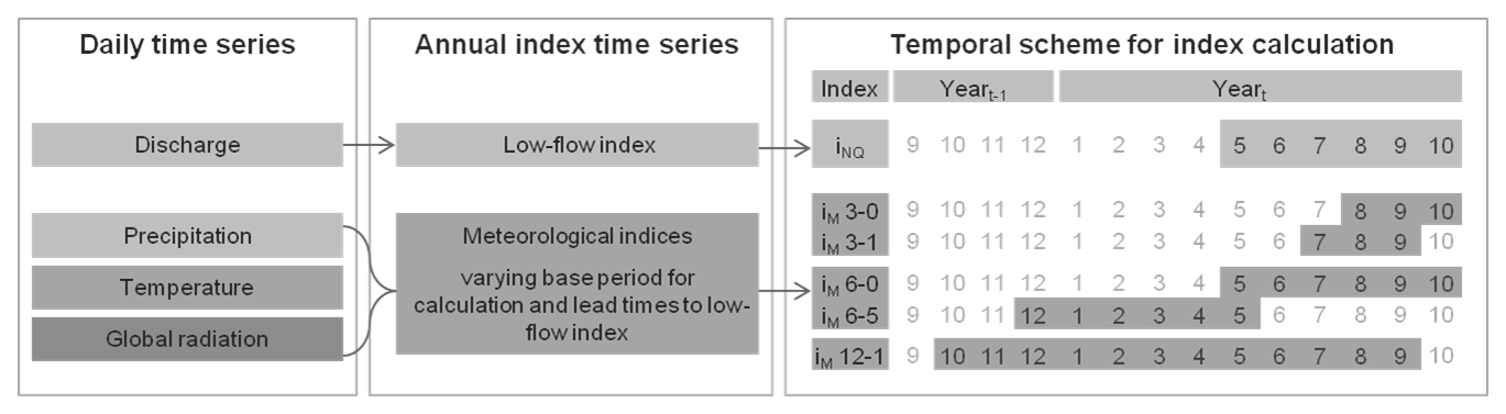
Figure 2 Calculation scheme for low-flow indices with a fixed base period and meteorological indices with a varying base period and lead times relative to the low-flow calculation period.

Table 2 Meteorological indices based on precipitation, temperature, and potential evapotranspiration.

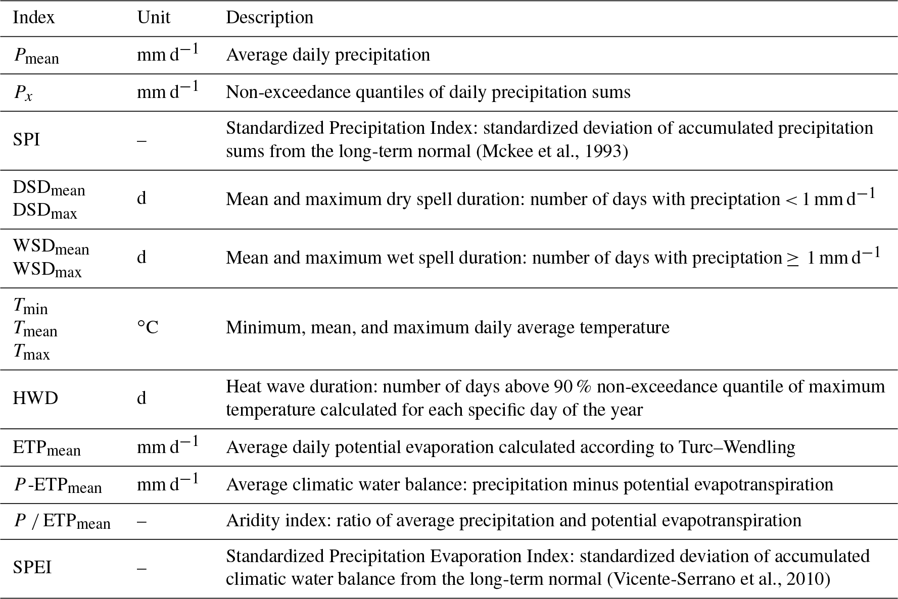
Meteorological indices are used as input for the models. Like for their low-flow counterparts, annual values are calculated from daily time series of precipitation sums, mean and maximum temperature, and global radiation, averaged over the respective basins of the considered discharge gauges. Table 2 summarizes the applied indices and gives a short description.

While the low-flow indices are calculated for a fixed period within the year (the summer half-year), the period for computation of the meteorological quantities is varied in length and position. Figure 2 shows the schema according to which every meteorological index has been computed. I_NQ represents the low-flow index, calculated for its fixed period within a given year. I_M denotes the meteorological index. The first number in the index notation represents the length of the base period for calculation (e.g., 3, 6, or 12 months), while the second one indicates the lead time, i.e., the number of months the period is shifted back in time relative to the low-flow index. A 0-shift indicates that the calculation period ends simultaneously with the low-flow period.

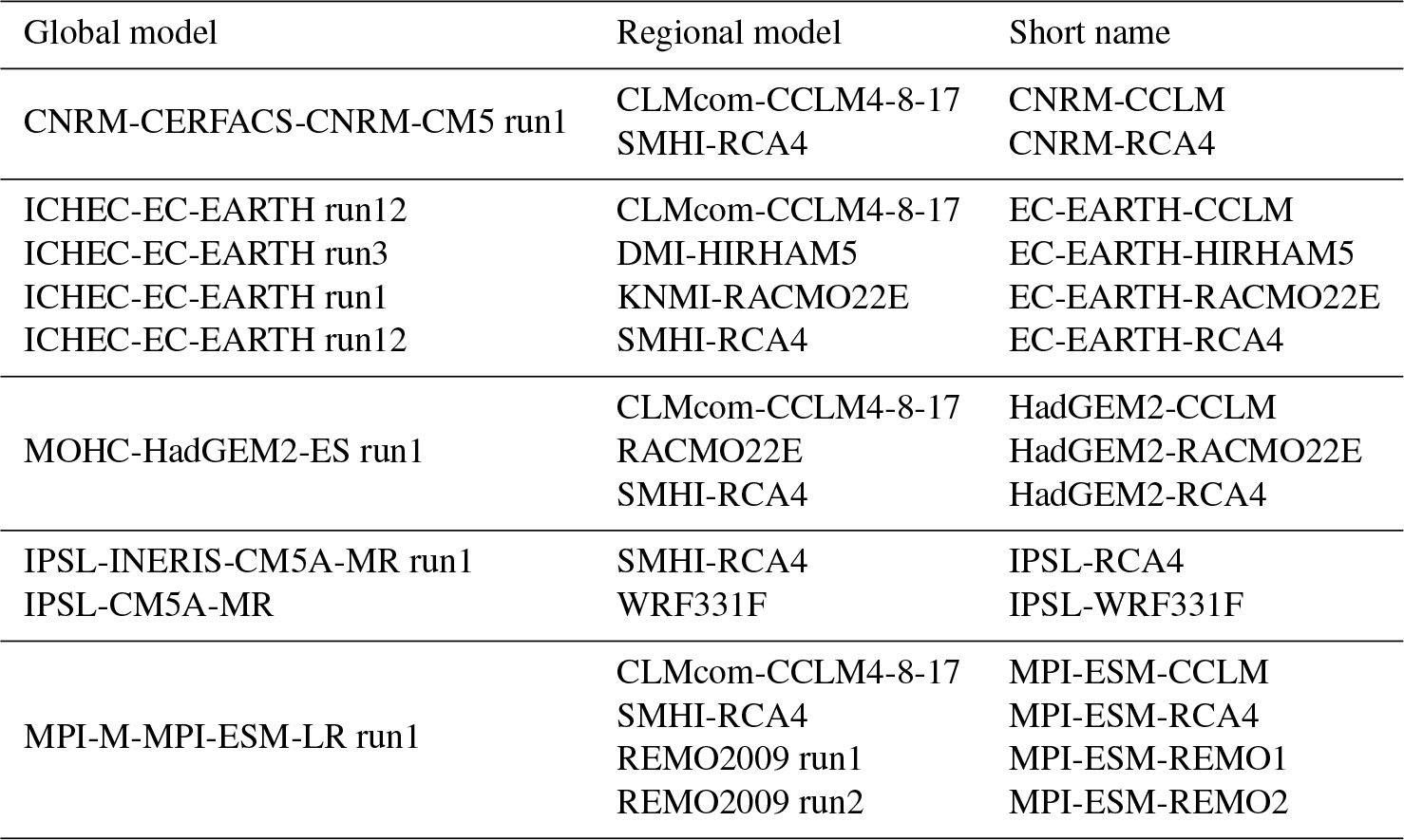
Table 3 List of coupled global and regional climate models used for analysis.

2.4 Climate model data

An ensemble of 15 coupled global and regional climate models is applied for climate change impact analysis. An overview is shown in Table 3. The datasets are based on simulations of global climate models of CMIP5 run on an RCP8.5 scenario. The data are available on a 10×10 km grid.

The climate model data have been pre-processed in previous work (NLWKN, 2017) and are available for a smaller domain than the observed climate data. Therefore, basin averages can only be computed for 17 of the 28 stations, as shown in Fig. 1.

3 Methods

The aim is to model a desired low-flow index on an annual basis as a function of a combination of meteorological indices observed in time. Several methods will be analyzed for this purpose in order to identify the one most suitable for modeling the relationships in consideration of their later application for far-future predictions. These methods are described in the following.

3.1 Multiple linear regression

Multiple linear regression (MLR) is probably the most common method to model relationships between variables and will pose the basis for several methods in this work. It aims at reproducing a target variable y as a linear combination of k explanatory variables x₁, … x_k. The general shape of a multiple linear regression model is the following:

$$\begin{array}{}\text{(1)}& y={\mathit{\beta }}_{\mathrm{0}}+{\mathit{\beta }}_{\mathrm{1}}{x}_{\mathrm{1}}+\mathrm{\dots }+{\mathit{\beta }}_k{x}_k+\mathit{\epsilon }.\end{array}$$

The regression coefficients β₁, … β_k are estimated in two different ways, i.e., (a) an ordinary least squares (OLS) procedure and (b) a generalized least squares (GLS) fitting. The latter method involves the inclusion of the covariance matrix of the residuals, which allows for correction for both heteroscedasticity and dependence of the residuals. Since heteroscedasticity did not appear to be a relevant issue in this study, while serial correlation in the data did, autoregressive (AR) covariance structures of various orders are tested to describe the residual covariance. The elements of an AR(1) covariance structure, for example, can be described via

$$\begin{array}{}\text{(2)}& {\mathit{\sigma }}_{ij}={\mathit{\sigma }}^{\mathrm{2}}{\mathit{\rho }}^{\left|i-j\right|},\end{array}$$

where ρ denotes the autocorrelation between terms with lag 1.

The need for and order of the considered AR process is determined using the likelihood ratio test on a case-by-case basis. This parametric test is developed to test the superiority of more complex models over their simpler forms, i.e., whether a model with a higher number of parameters performs significantly better than the same model with fewer parameters. Performance is thereby measured in terms of maximized log-likelihood function values and the (1−α) quantile of the Chi² distribution, whose degrees of freedom are chosen as the difference in the number of parameters between the compared models (Coles, 2001).

3.2 Principal component analysis

The fitting of multiple linear regression models is restricted by sample size. Fitting a model with a large number of regressors to a small data set will result in over-fitting. Additionally, the problem of multicollinearity between the explanatory variables in a model arises. As such, for a small data set, only a small number of uncorrelated regressors should be selected. At the same time however, leaving out important explanatory variables may drastically lower the predictive power of the model. In order to overcome the restrictions given through the limited period of observation, a principal component analysis (PCA) is applied, merging many explanatory variables into a few uncorrelated components that pose the ideal basis for model fitting on limited data with maximum exploitation of information. PCA is carried out by firstly centering the set of p explanatory variables X^* via subtraction of their respective means. Then, the (p×p) covariance matrix Σ is computed and its eigenvalues λ₁, λ₂, … λ_p and eigenvectors γ₁, γ₂, … , γ_p are determined. Multiplication of the eigenvectors with X^* yields the following system of equations:

$$\begin{array}{}\text{(3)}& \begin{array}{c}{y}_{\mathrm{1}}={\mathit{\gamma }}_{\mathrm{11}}{x}_{\mathrm{1}}+{\mathit{\gamma }}_{\mathrm{21}}{x}_{\mathrm{2}}+\mathrm{\dots }+{\mathit{\gamma }}_{p\mathrm{1}}{x}_p\\ y_{\mathrm{2}}={\mathit{\gamma }}_{\mathrm{12}}{x}_{\mathrm{1}}+{\mathit{\gamma }}_{\mathrm{22}}{x}_{\mathrm{2}}+\mathrm{\dots }+{\mathit{\gamma }}_{p\mathrm{2}}{x}_p\\ \mathrm{⋮}\\ y_{\mathrm{p}}={\mathit{\gamma }}_{\mathrm{1}p}{x}_{\mathrm{1}}+{\mathit{\gamma }}_{\mathrm{2}p}{x}_{\mathrm{2}}+\mathrm{\dots }+{\mathit{\gamma }}_{pp}{x}_p\end{array},\end{array}$$

where y₁, y₂, … , y_p denote the principal components, sorted according to their contribution to the total variance of data at hand. The eigenvectors represent the respective loading of a variable x on a principal component y.

Figure 3 Vertical structure of the HBW-IWW model according to Wallner et al. (2013).

3.3 Hydrological modeling

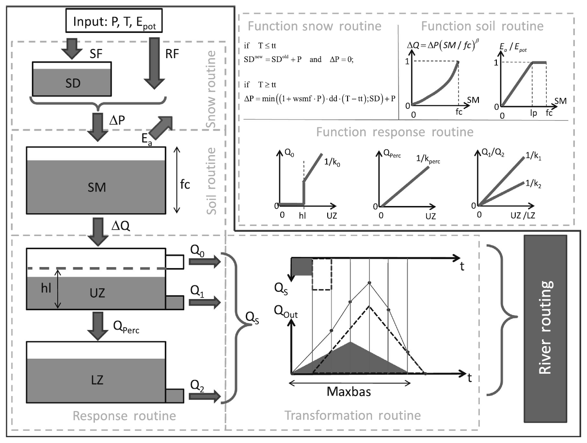
In order to evaluate the performance of the statistical approaches, hydrological modeling is applied as the benchmark for prognosis of future flow. The rainfall–runoff model used here is an adaptation of the Swedish HBV by Lindstrom et al. (1997), denoted HBV-IWW. The specifics of the model are described in detail, e.g., in Wallner et al. (2013). A schematic overview of the structure of the model is presented in Fig. 3. The model is semi-distributed and can be applied on the sub-catchment scale. Input is daily precipitation, temperature, and potential evapotranspiration. The model comprises five routines and a variety of parameters controlling the translation between the various model components. The parameters are automatically optimized using the AMALGAM evolutionary multimethod algorithm (Vrugt and Robinson, 2007).

3.4 Model fitting and evaluation

Given the vast number of meteorological indices, variable selection for the statistical models becomes paramount. In order to select appropriate indices and restrict the numbers of selected regressors, a two-way stepwise approach for variable selection is chosen that aims at minimizing the Bayesian information criterion (BIC; Schwarz, 1978) of the final model. The BIC is closely related to the Aikaike information criterion (AIC; Aikaike, 1974) but penalizes variable inclusion stricter for larger sample sizes, which is the reason for its selection in this study. The smaller the BIC, the better the predictive power of a model. The algorithm for variable selection randomly selects a variable and adds variables to the model that decrease the overall BIC. After each addition it is tested whether the removal of any of the existing variables in the model leads to further decrease in the BIC.

Since the number of potential regressors in this study is high and variables may be strongly related, a second criterion is included in the BIC-minimization procedure. In order to prevent multicollinearity, the variance inflation factor (VIF) of each variable added to the model is computed. The VIF is a measure of how much of the variance of a predictor in a model can be explained by the other predictors in the same model. Computation is done via

$$\begin{array}{}\text{(4)}& \mathrm{VIF}={\displaystyle \frac{\mathrm{1}}{\mathrm{1}-R^{\mathrm{2}}}},\end{array}$$

where R² denotes the coefficient of determination of a regression model that describes the variable to be added as a function of the existing variables in the model. The recommended limits for the VIF vary throughout literature. Since multicollinearity is a major issue for the analyses of this study, a low value of 5 has been chosen. Variables that show higher VIFs are not included into the existing model.

For the GLS models with AR-correlation structure, variable selection was carried out according to OLS model fitting, evaluating the necessity of the AR-structure for each added variable using the likelihood ratio test. For variable selection using principal components, the BIC-minimization strategy is extended, not by adding each additional variable directly to the model but by computing principal components first and testing them as potential regressors of the model.

In contrast to the statistical models, the hydrological model is based on daily input and output and is therefore capable of modeling an entire year's hydrograph rather than a single low-flow metric. Calibrating the hydrological model on the complete hydrograph may reduce the predictability of the single low-flow event and favor the statistical models (directly calibrated on the low-flow value) in a comparison of model performances. Therefore, the HBV-IWW is calibrated in a strategy comparable to the statistical approaches, namely by including nothing but the desired annual low-flow metric in the objective function.

In order to allow for a proper assessment of the models' capabilities of predicting future low flows, the available record at each station is split equally into a calibration and a validation period. Both periods are continuous in time and the calibration consistently precedes the validation period. This setup is chosen to test the ability of models fitted to a past period of time to predict “future”, i.e., the validation period's characteristics. In order to double the available periods for validation, the time series are inversed and models are fitted to the former validation period and evaluated in the calibration period. The inversion is applied in order to preserve the continuity of the time series.

In order to compare the quality of the different model approaches, a selection of performance measures is computed. These measures include the coefficient of determination (R²), the normalized root mean square error (NRMSE), and the percent bias (pbias). The criteria are selected to show various aspects of model quality, i.e., information about the similarity of the course of simulated and observed time series, the average fit, and systematic errors.

3.5 Climate change impact analysis

The most suitable statistical model is eventually applied using the ensemble of climate model data. The first step is the assessment of the performance of the model chains in reproducing the observed low flow. This analysis is done in a reference period from 1971 to 2000. The projections and changes in the low flow will be analyzed in near- (2021–2050) and far-future (2071–2100) periods. It should be noted that the aim of the prognosis using actual climate model data is primarily for the validation of the statistical model approaches rather than a detailed regional assessment of expected changes.

In order to account for potential bias in the climate model data used for prediction of future low flow, the individual station models are recalibrated for each climate model separately. The problem that needs to be overcome for this process is the matching of the temporarily dissociated series of meteorological indices generated by the climate models with the observed low-flow time series, which is handled as follows. At first, the explanatory variables identified in the observed model fitting procedure are carried over; i.e., no new variable selections are carried out. This is meaningful, since the selected variables represent observed low-flow drivers. The principal components are then re-estimated for the selected variables as projected by the individual climate models. In order to relate the climate model data to the observed time series, the regression parameters are optimized in such a way that the empirical distribution of the predicted low flow matches that of the observed sample. In order for the recalibrated model to be no more precise than the originally fitted model, which may lead to false estimates of the regression coefficients, the model fitted to the observed data is used as the target during re-calibration rather than the observed low-flow series itself.

4 Results and discussion

4.1 Model performance

Performance of the individual MLR model variants are compared using the aforementioned performance measures. Figure 4 shows the model performance of all tested model configurations exemplary for NM7Q prediction in the calibration (top) and validation period (bottom). For the validation period one can clearly observe an increase in performance from left to right, i.e., an increasing predictive power with increasing model complexity. The OLS-fitted model shows poorest performance with a median R² of only 0.43.

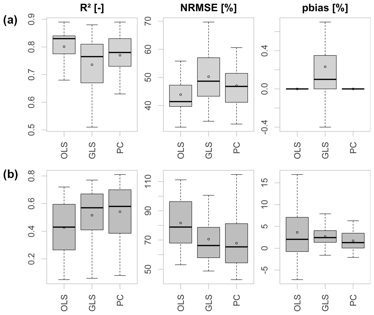
Figure 4 Performance criteria of different model approaches in the calibration period (a) and validation period (b) over 28 stations.

The highest predictive performance has been achieved with the principal component model. The coefficient of determination for the MLR model over all stations has a median value of 0.58. The PC model also shows the smallest percent bias with a median of 1.30 %. The inclusion of several variables in the form of principal components appears meaningful in order to avoid omittance of important regressors and potential multicollinearity, granted by the orthogonality of the components. Additionally, the principal component models are supposedly more robust against outliers in single variables.

The second best performance is shown by the GLS-fitted model with an AR-correlation structure. One should note that an AR-correlation structure has not been used for model fitting at every station. Only at those stations where the likelihood ratio test favored an inclusion was a GLS fitting carried out. This was the case for 55 % of the fitted models (35 % AR(1) covariance structure, 20 % AR(2) covariance structure). The bias in the calibration period arises through the approximation of the unknown true autocorrelation structure in the data. Since the values are negligibly small, this approximation is considered reasonable. As the number of variables included in the GLS model is significantly lower compared to the principal component model, and the step of finding suitable components was skipped, the performance based on the close validation period, as shown here, appears to be comparably good. However, inclusion of AR processes via likelihood ratio testing results in some distortion of the residuals and violation of the prerequisites of linear regression fitting at several stations. Thus, the principal component model is considered favorable.

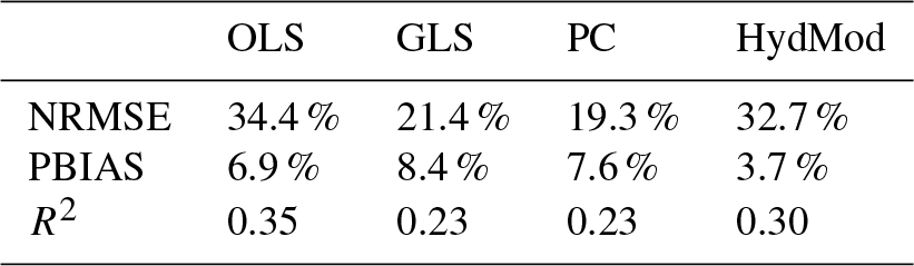
Figure 5 shows the same criteria as Fig. 4 with inclusion of the hydrological model, and thus for a total of seven stations only. The performance of the HBV model in both calibration and validation periods is substantially better in all aspects, with a median validation R² of 0.50, an NRMSE of 76.1 %, and a percent bias of 1.7 %, compared to the PC model with median values of 0.42 %, 78.4 %, and 5.8 %, respectively. This performance however could only be achieved using the calibration strategy of matching exclusively the annual NM7Q values at each station. Calibration using the entire hydrograph or parts of the flow duration curve did not explicitly outperform the statistical approaches. Nevertheless, HBV-IWW appears to be suitable for assessment of future low-flow development when calibrated specifically on low-flow indices.

Figure 5 Criteria for goodness of fit of different model approaches in the calibration period (a) and validation period (b) over seven stations.

The statistical models appear to be positively biased. At almost all investigated stations a positive mean error could be observed. As models are fitted in both directions to the time series, this error appears to originate in the model itself, rather than in underlying processes of the time series that cannot be captured. Overall differences in model performance between the stations could not be correlated with any specific regions or catchment features. The quality of the simulation did not depend on catchment size, position in the study area, or any other distinguishable factor.

An obvious problem is the significant difference in model performance between the calibration and validation periods. All quality criteria certify a much better performance during calibration than during validation. Tables 4 and 5 show the median differences in goodness-of-fit measures for all model variants over all stations and over the stations at which hydrological modeling was possible. The differences are severe, even though quite a number of precautions have been taken during calibration. The R² for PC, for example, differs by 0.22 between calibration and validation. For the seven stations this difference increases to 0.23. Overfitting appears to be an issue, even though the number of regressors has been restricted. However, the differences are also observable for the hydrological model, in some cases even more drastically than for the statistical models. The median difference in R² over the seven stations is 0.3 between calibration and validation periods.

Table 4 Median absolute difference in quality criteria between calibration and validation period for 28 stations.

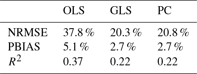
Table 5 Median absolute difference in quality criteria between calibration and validation periods for seven stations.

Through separation of the validation period into three parts it becomes obvious that performance decreases steadily with distance from the calibration period, as shown in Fig. 6. Compared are the estimated and the observed means for all statistical methods. The effect shows that non-stationary relationships between low-flow and meteorological indices are of major relevance and need to be considered in statistical modeling. Logically, with a changing climate, interrelationships between individual meteorological variables and hence the ratio of the influence of individual drivers on low-flow formation will change. At the same time, other forcings and feedbacks may become more or less relevant, which have not been included in the statistical model formulation in the first place. In an initial attempt at encompassing the problem by addressing a potential linear time dependence of the regression coefficients, the parameters have been re-estimated as linear functions of time using a maximum likelihood fitting. The required complexity of the models has been assessed using likelihood ratio tests. However, model fitting appeared problematic for the small calibration period and did not yield an improvement of the existing models.

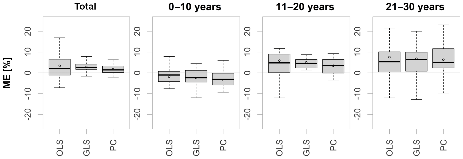
Figure 6 Mean deviation of estimated from observed means for the whole validation period (left), as well as the first, second and final 10 years of validation.

It should be noted that the model set up for calibration and validation allows for assessment of changes between directly adjacent periods only. Application of the models to predict low flows in a more distant future under more severe climatic change may significantly enhance the error due to non-stationarity.

Apart from the non-stationary relationship between target variable and regressors, another possible explanation – especially with respect to the observations regarding the hydrological model – could be a significant difference in flow behavior between the two periods selected for calibration and validation, potentially caused by forcings other than the local climate. A previous study by Fangmann et al. (2013) has found that time series at a majority of gauges in the study area are divided by significant break points (according to Pettitt, 1979) between the years 1987 and 1989. Since neither the hydrological nor the statistical models involve input other than the local meteorology, this break cannot be accounted for by either approach. Also, anthropogenic interference poses a relevant factor. Even if indirectly considered in the statistical models, changes in the management patterns would significantly alter the prognosis; a factor that needs to be considered during model application.

Modeling of the other tested indices showed quite a differentiated picture. As shown exemplarily for seven stations and the GLS approach in Fig. 7, some indices were reproduced more successfully (top) and others less so (bottom) than the NM7Q. Estimation of the Q₉₅ appeared slightly better in terms of all quality criteria. The D_max was modeled effectively via GLS in terms of R² and NRMSE (median values of 0.54 % and 80.8 %), but showed quite a large bias. V_max and especially the annual low-flow timing could not be modeled successfully by any of the statistical approaches (median R² of 0.31 and 0.03, respectively).

Figure 7 Validation results for the GLS model and the hydrological model for various low-flow indices at seven stations performing better (a) and worse (b) than for the NM7Q.

It was noted that the overall model performance was slightly higher for the more average values, i.e., NM30Q and Q₈₀, than for the more extreme indices NM7Q and Q₉₅. The median R² values of the NM7Q and the NM30Q compare as 0.47 and 0.52, the ones of the Q₉₅ and Q₈₀ as 0.49 and 0.62. Compared to the D_max and V_max, the annual average D_mean and V_mean cannot be predicted by the fitted models. The validation yields R² values below 0.1 for both cases.

The differences in reproducibility of the various metrics can be explained by the nature of the indices and the structure of the statistical models. The regression model uses aggregated meteorological features over a specific period of time for prediction of a desired low-flow variable. The shorter the required period, the lower the degree of averaging and the greater the possibility of capturing extremes that cause a subsequent low-flow event. Therefore, indices related to a specific event, like the NM7Q or the D_max, can be modeled quite effectively based on previous meteorological states. The fact that more average indices like NM30Q and Q₈₀ are reproduced better than more extreme ones can be explained by the same principle. Meteorological indices computed for longer base periods are required to model more average index values. Errors that occur if extremes cannot be explained by external variables are lower. D_mean and V_mean, however, do not represent averages of single but of multiple events. These features cannot be captured by small sets of regressors as used in this study.

Alongside the validation results of the statistical models, those of the hydrological model are presented in Fig. 7. The indices in the top panels are deduced from the simulation runs of the models that were calibrated on the annual NM7Q. In order to better represent the indices related to duration and volume, the model used in the bottom panels was calibrated using the annual V_mean as a fitting criterion. One can see that the results for all indices improve for the hydrological model as expected, due to a more detailed process representation. This is especially the case for the average duration- and volume-based indices. Still, the differences in performance for the individual indices are visible also for the hydrological models.

It should be noted that the selected statistical methods exclusively take linear relationships between target variable and regressors into account. It appears that these linear dependencies are strong, and major portions of the variance in the target variables could be explained by the fitted models. At this point it cannot be precluded that nonlinear relationships with some meteorological indices do exist, but it is presumed that important influential quantities can be linearly related to the target variable. It is well considered that such relationships may change under future conditions that deviate strongly from the present circumstances under which the statistical models were fitted. As discussed above, the statistical models can only be evaluated in a validation period directly adjacent to the calibration. Most hydrological models, which involve much greater detail in physical process representation, will more certainly be transferable to situations where interrelationships between low flow, meteorology, and other influencing factors are altered. The actual capability of the statistical approaches in estimating future low flow as mere functions of future climate would need to be assessed, e.g., using simulation studies involving “past” and “future” runoff simulated by a hydrological model. Such an experiment is beyond the scope of this study, but may be a useful test for further studies.

4.2 Low-flow drivers

The PC models are used to evaluate the selected explanatory variables over all stations. For the NM7Q, the majority of models comprise one or two principal components made up of two to eight meteorological indices. Many of the selected variables repeat for most of the models. The most common predictors of the NM7Q appear to be the aridity index P ∕ ETP for 3- and 6-month base periods and for 1–4-month lead times, as well as the P-ETP for the same periods. The second most frequent regressor is the SPI of various base periods and lead times (0 to 3 months). Upper precipitation quantiles with various base periods and lead times follow in frequency. Several models also contain DSD and the ratio between average DSD and WSD as predictors. Pure temperature-based predictors are rare, but do occur in some cases. The selected lead times of the temperature-based indices are in these cases larger than for the precipitation or water balance indices. Lead times as long as 9 months, which would represent November–January temperature, are observed. Winter temperature hence appears to be an important predictor for summer low-flow magnitude.

The inclusion of indices with differing base periods and lead times at the individual stations represents the heterogeneity of transformation processes within the study area. One of the major determinants of how meteorological processes translate into flow is catchment size. Larger, rather slowly responding catchments with significant storage capacity will less likely be affected by small meteorological events and low flows will occur moderated and with significant temporal delay. Therefore, statistical models fitted for these catchments will most likely include meteorological indices that have been computed for longer base periods and lead times. Within small, quickly responding systems on the other hand, low-flow magnitudes may be related to shorter dry periods that have occurred recently. Variable selection is thus carried out in favor of small base periods and lead times. Nevertheless, even for smaller catchments an inclusion of temporally leading meteorological indices may mimic initial storage conditions and determine the absolute magnitude of a summer low-flow event.

The models fitted to the NM30Q are comparable to the ones of the NM7Q but contain on average fewer explanatory variables per model. As discussed before, the more average low-flow values are more easily predicted, apparently requiring less external information. In contrast to the NM7Q, temperature-based indices do not appear to be important predictors of the NM30Q. Considering the models of the other indices, it can be seen that the selected regressors differ between the individual types. While Q₉₅ and Q₈₀ are primarily predicted by water balance parameters, as are the NM7Q and NM30Q, the models for D_max and V_max count a high number of indices related to durations, especially average and maximum dry spell duration. The regressors selected for the forward and inversed fitting carried out at each station are not always identical. Some of the independent variables are naturally very similar for various base periods and lead times so that they are almost exchangeable, which in turn makes the fitted models very similar. Still, this observation hints again at the problem of non-stationarity and the observed breakpoint near the transition between calibration and validation periods.

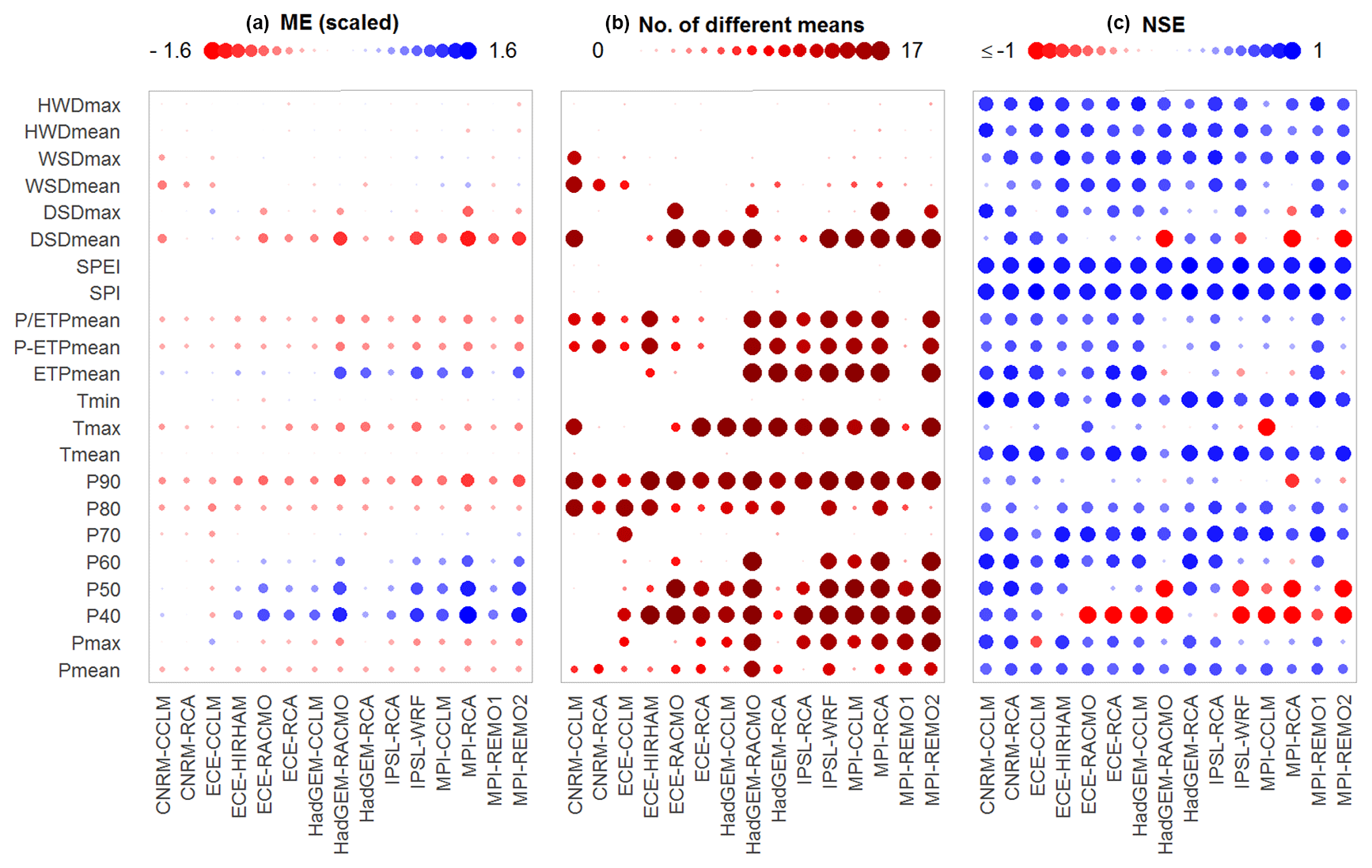
Figure 8 Comparison of simulated and observed meteorological indices for each model over 17 stations: mean error (a), number of significant shifts in location (b), and Nash–Sutcliffe efficiency of ordered series (c).

4.3 Prognosis

For prognosis, the principal component models are applied using the ensemble of climate model data described above. For reasons of conciseness only the NM7Q is selected as the target variable in this example and only changes in the means for the near- and far-future periods are assessed. In order to firstly evaluate the climate models' capabilities to reproduce the required input variables for the impact models, the meteorological indices obtained from the models are compared to the observation in the reference period. Figure 8 summarizes the results. Three measures are used to assess the models' capability to reproduce the indices: (a) the mean error, i.e., the difference in means between simulation and observation over all stations (computed for scaled data to make it comparable between indices); (b) the number of stations where this difference is significant at a 5 %-significance level, tested using a non-parametric Mann–Whitney test (Wilcoxon, 1945); and (c) the NSE of the simulated and observed index time series, both ordered by size, as a means of assessing the similarity of the two distributions. The indices considered in the plot are calculated on a 6-month base period with a 3-month shift and are representative of most base periods and lead times.

The left panel shows that deviations are observed for the climatic water balance and the aridity index, i.e., average P-ETP and P ∕ ETP. The climate models consistently underestimate the observed values. What also becomes apparent is that upper precipitation quantiles (P70–P90) are mostly underestimated. The amount of significant differences found for the means, especially in P90, suggest that there is a significant bias throughout the study area. Additionally, the NSE values are rather low, indicating a generally poor reproduction of these index values. Apart from the quantiles and the climatic water balance, errors are found for maximum temperature and dry spell durations. The lower precipitation quantiles show quite high errors but are rarely considered in the station models. For those variables that are considered, additional bias correction may be advisable.

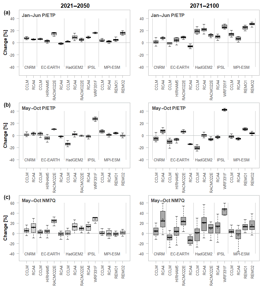
Figure 9 Projected changes in winter (a) and summer (b) aridity index and NM7Q (c) by all models over 17 stations and two future periods.

The climate models appear to have limited ability to reproduce some of the true meteorological indices. This effect may be due to the inability of the regional climate models to downscale the global climate data appropriately for the study area. One also needs to consider the difference in grid size between the observed data, which has a detailed 1 km resolution, and the simulation, which is available on a 10 km grid. Since mere averaging of the grid cells has been applied to obtain the basin averages, the smoothing effect may be recognizable, especially for small catchments and in heterogeneous terrain. The re-calibration technique described in Sect. 3.5 was chosen to address these issues related to various forms of scaling.

Figure 9 shows the prognoses of the individual climate models over all stations. Along with the summer NM7Q (bottom), projections for the aridity index are shown, as they indicate the overall climatic development. Also, the index is included in numerous stations' impact models. The index's development is shown for a 6-month base period without lead time, which equals the computation basis for the NM7Q (May–October; center) and a 4-month shift (January–June), which equals the maximum lead time considered in the station models (top).

The changes for January–June P ∕ ETP are predominantly positive for the majority of models and stations. Only the EC-EARTH coupled with the CCLM and the RCA4 show negative trends. The total range of projections is −13.31 % to +34.10 % in the far-future period. The positive change in the ratios is caused by a significant increase in January–June precipitation amounts, projected for all stations by all climate models, which exceeds the simultaneously projected increase in evapotranspiration. For summer, the projections for the P ∕ ETP are more ambiguous. Nine ensemble members clearly predict a significant decline in the far future, while five models project an increase at all considered stations. The spread of the projection is accordingly large, ranging from −25.75 % to +48.91 %. The IPSL-WRF331F thereby shows by far the highest positive development and can potentially be considered an outlier. The rather negative trend in the summer P ∕ ETP is related to both decreasing precipitation, as projected by most models, and increasing evapotranspiration.

For the NM7Q the spread of changes over the considered stations is significantly larger and increases further from the near- to far-future periods. This is a logical consequence, since flow behaves much more heterogeneously throughout space and direction and magnitude of change may greatly depend on local conditions. Overall, the changes in the NM7Q appear to be a mixture of the patterns observed for P ∕ ETP in both summer and winter. The highest increase in NM7Q is predicted by the IPSL-WRF331F model chain (median 48.18 %), which also shows highest increase in precipitation amounts and strongest decrease in evapotranspiration in both summer and winter. EC-EARTH-CCLM and –RCA4 predict the strongest decrease (median −7.9 % and −13.42 %, respectively), which is also in accordance with declining P ∕ ETP in both summer and winter. Apart from these models, there appears to be a general increase projected for summer NM7Q over the majority of stations. It seems that on average the influence of spring and winter meteorological states weighs stronger on the formation of summer NM7Q than the actual summer conditions.

Figure 10 shows the spatial distribution of the projected changes for the two future periods and the variables analyzed previously. Depicted are the median changes over all climate model ensemble members for the individual stations. All stations show an average increase in winter P ∕ ETP ranging from +6.84 % to +14.75 % in the far future. At the majority of stations a decrease is projected for summer, with the largest changes occurring in the Harz mountains, i.e., the most southeastern stations in the study area, with an average decrease of −4.72 %. Positive changes can be found in the northern stations, with up to +3.12 % in the near future but decreasing to +2.76 % in the latter period. The NM7Q is projected to increase by up to 22.79 % at all but four stations, where a median decrease of up to −12.01 % is projected. Two of these stations are situated in or near the Harz mountains, where flow-forming processes and climate are quite different from the rest of the study area. Additionally, their areas are the smallest in the data set considered for impact analysis (44.5 to 363.0 km²). Apparently, the NM7Q in these areas is influenced more by summer meteorology than the rest of the study area.

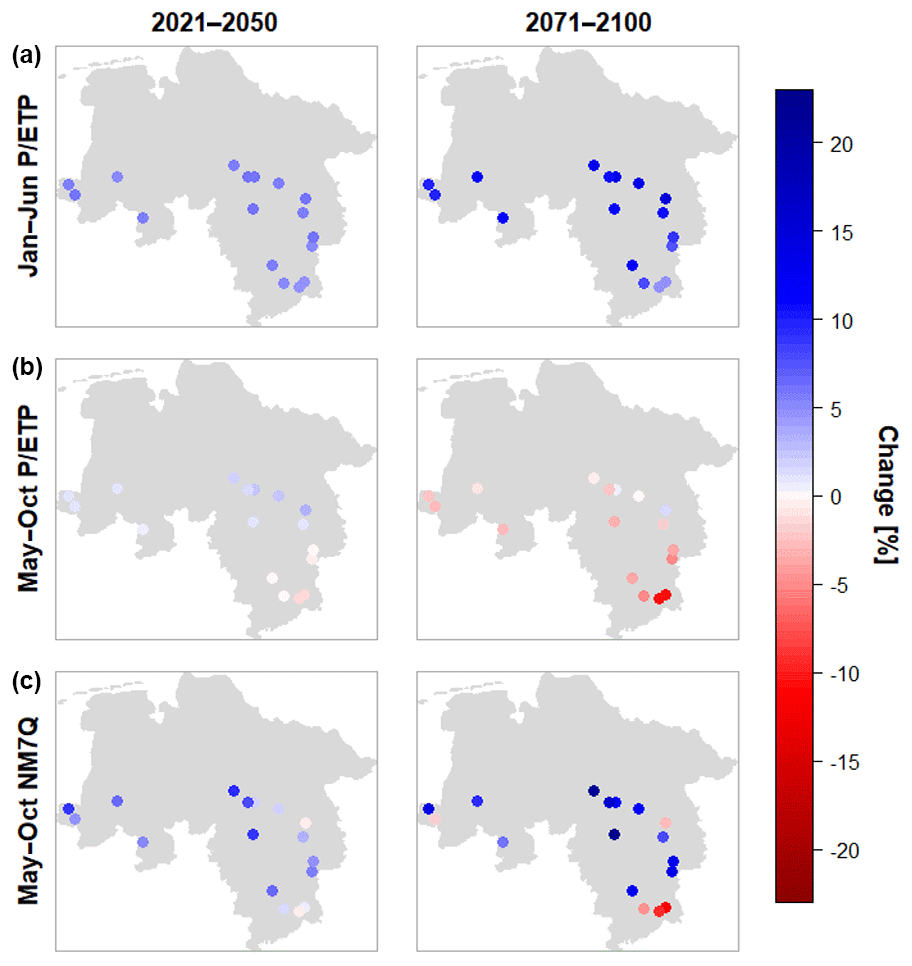
Figure 10 Medians of projected changes in winter (a) and summer (b) aridity index and NM7Q (c) by for individual stations over 15 climate models and two future periods.

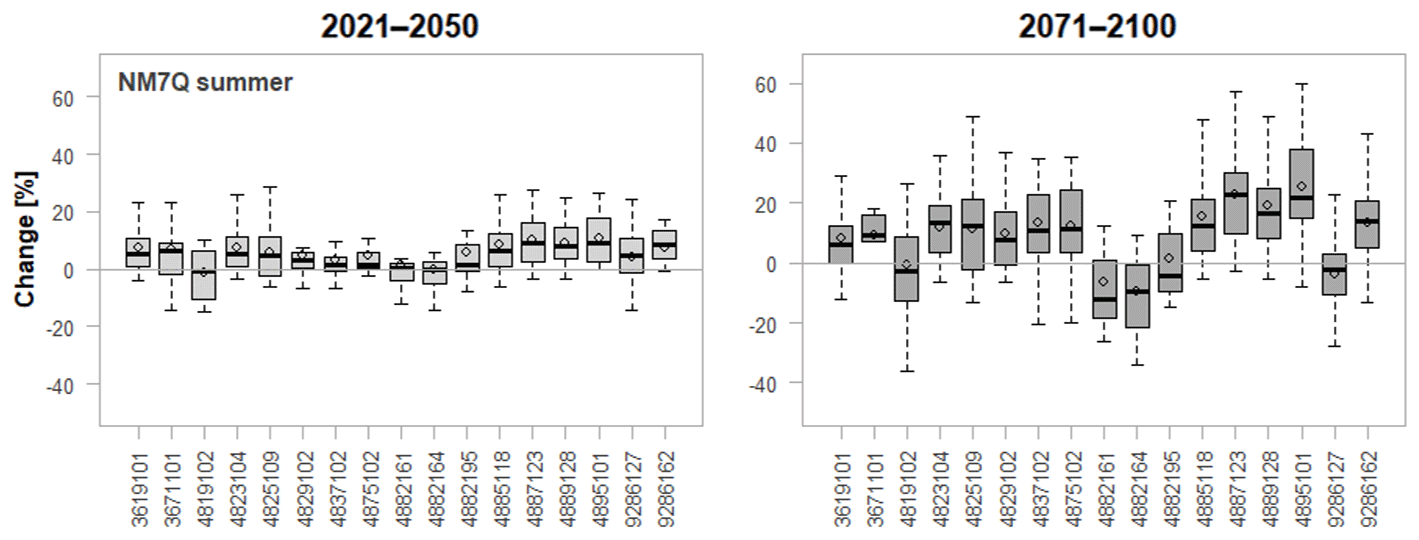
Figure 11 Projected changes in summer NM7Q for individual stations over 15 climate models and two future periods.

Finally, Fig. 11 shows boxplots for all stations and the projected changes in the NM7Q over all considered ensemble members. It can be seen that at most of the stations the predicted directions of change are quite unambiguous over the majority of climate models, and projections are accordingly quite robust. Exceptions are stations 4819102, 4882195, and 9286162, where the median change is close to 0. What also becomes apparent in these plots is the spatial dependence between stations. Identical leading digits of the station numbers indicate that stations belong to the same river basin, while increasing numbers indicate more downstream locations, i.e., larger size, as depicted in Fig. 12. The projected changes are obviously strongly related to catchment area, since continuous transitions are observable from most negative/smallest change in NM7Q at the smallest to most positive change at the largest catchments within each basin. Summer low flow in catchments with large storage capacity will more likely be influenced by the increasing annual and winter precipitation amounts, while the flow in the smaller catchments is more drastically influenced by drier summer meteorological conditions. It remains to be analyzed, e.g., via hydrological modeling, whether this observation is an artifact created by oversimplification of the statistical approaches (through neglect of other relevant, potentially counteracting factors) or a truly observable phenomenon. Nonetheless, the coherence of the projected station means suggests that the statistical models – even though they have been fitted independently for every station – exhibit a meaningful spatial consistency within the region. Apparent outliers are not produced by any stations' statistical impact model.

Figure 12 Catchment areas of the considered gauges.

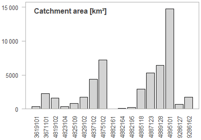
Figure 13 Projected changes in winter NM7Q for individual stations over 15 climate models and two future periods.

The significant increase in winter and partly projected decrease in summer P ∕ ETP may suggest a temporal shift in minimum flows from summer/early fall to late fall/early winter in the study area. In order to test this hypothesis, statistical models are fitted to additionally model the winter NM7Q. Modeling of the winter values was more difficult than of the summer low flows since their causes may not be representable by the utilized indices (e.g., water retention by snow). The final projections in Fig. 13 suggest that the expected developments for winter are less conclusive than for summer. At most stations mostly positive trends are projected for both future periods with lacking robustness. A pronounced pattern of change contrasting the summer NM7Q cannot be observed. Accordingly, with overall increasing precipitation amounts, the intensities of the severest events of the year are expected to decrease at most stations in the area, regardless of their time of occurrence.

Still, the findings indicate that there might be a slight delay in the onset of future low-flow events. The ratio of winter to summer low flows appears to increase slightly at most stations, while for the observation 10.20 % of the annual lowest low-flow events occur in winter, the models predict on average 15.1 % for the reference period, 20.00 % for the near and 22.67 % for the far future.

A comparison of the signals projected in this work to other studies that analyze comparable regions and climate model ensembles but use hydrological models for impact assessment is difficult, due to differences in scale, model ensemble, and type of analysis (e.g., based on degree of heating rather than on fixed periods). A regional study that is comparable to this work has been carried out by Osuch et al. (2017) for Poland. They investigated climate change impacts on low flows, including the annual NM7Q, using the HBV model and, among others, an RCP8.5 climate model ensemble. They found significant positive changes in the NM7Q for the RCP8.5 scenario, with a more than average 40 % increase in the study area in a period from 2071 to 2100. These changes are much larger than the ones found in this study but are obtained for a more continental climate. Other studies analyzing climate change effects on low flows over the whole of Europe (e.g., Marx et al., 2018) or global studies (e.g., Wanders and Yada, 2015) using RCP emission scenarios usually find inconclusive changes in low-flow magnitude for the northwestern parts of Germany (between −10 % and +10 %). The average changes in the annual NM7Q over all stations and ensemble members obtained in this study are +5.62 % for the near- and +8.96 % for the far-future periods, and are thus within the range of these findings. Van Vliet et al. (2015) show in their Europe-wide study that especially in central western and northern Europe the projected changes in streamflow drought under an RCP8.5 scenario appear to differ between the two hydrological models they applied, both in direction and magnitude. In general, it appears difficult to assess future low-flow development in the region, especially in comparison to the parts of Europe where expected changes in precipitation are more pronounced and unequivocal between climate models.

5 Conclusions and outlook

The aim of this work was to assess key low-flow drivers using simplified statistical approaches. Several regression models with varying restrictions and assumptions have been set up and evaluated in a split-validation procedure. In order to assess potential future changes in the low flow, the models are applied to an ensemble of climate model data. The main findings are the following.

• Modeling of low-flow values as a function of meteorological indices appears feasible. An approach using just a few principal components of several variables as regressors yields the best results for the 60-year observation period. It showed to simultaneously countervail problems with multicollinearity and omittance of important explanatory variables.

• Non-stationarity within the relationship between meteorological predictors and low-flow target variables appears to be an issue, resulting from the entire neglect of physical processes and changing interrelationships between explanatory metrics. This problematic needs to be considered, when applying the models to future data, especially in terms of parameter stability. Ideally the models should be revised through inclusion of methods to map potential non-stationary processes and interrelationships.

• More average low-flow indices are reproduced better by the statistical models than their more extreme counterparts, e.g., the NM30Q compared to the NM7Q. Maximum duration and deficit volume can be adequately modeled, while the onset of an event can by no means be predicted by the suggested models.

• The main drivers for all low-flow characteristics are metrics related to precipitation and evapotranspiration amounts. Temperature indices appear to be relevant at some stations for certain low-flow metrics. Usually base periods for computation and lead times of the explanatory variables considered in the station models depend greatly on catchment size and response time of the catchments.

• The hydrological model outperforms the statistical approaches, when explicitly calibrated on the low-flow events.

• Both the statistical and the hydrological model show a major discrepancy in their performances between the calibration and the validation periods. This indicates a lack in capturing non-stationary processes or the presence of a significant non-homogeneity between the calibration and validation period considered for analysis.

• Applying the principal component model with an ensemble of coupled global and regional models based on an RCP 8.5 scenario yields on average an increase in summer NM7Q at most stations. Only two small headwater catchments show a decrease in NM7Q in the far future. These stations appear to not be influenced by preceding winter precipitation.

• A major weakness of the proposed model type is the reproduction of meteorological indices by the climate models. However, underestimation of the climatic water balance and upper precipitation quantiles may be a likewise limiting factor within process-based impact models. A direct calibration using climate model data instead of the observation can potentially help increase the quality of the projections made by the statistical models.

There are potential advantages to applying statistical approaches that have not been discussed before. One is that the required input consists of variables that are lumped over a significant amount of time (3–12 months). Such averages can potentially be better reproduced by climate models than the daily variability required for other impact model types. Also, the statistical models may be easily extended to include other forcings like large-scale phenomena, which may be similarly described by indices like local meteorological conditions. Land-use feedbacks also might be includable to some extent. What remains difficult to achieve is to statistically model feedbacks between different external variables with the simplified approaches. This problem may however be moderated by including non-stationary regression coefficients for individual variables. Considering issues with the coupling of global and regional climate and impact models (e.g., Dai et al., 2013; Wilby and Harris, 2006), including issues with downscaling, a direct use of large-scale teleconnections, and the possibility of applying the models directly to extrapolated climate data – rather than just climate model data – may suggest that statistical approaches can significantly increase the robustness of predictions. This is especially relevant when considered in an ensemble of various model types and information sources, as suggested by Laaha et al. (2016) for proper assessment of climate change impacts on low flows.

The statistical approach can also make use and benefit from inclusion of spatial information, especially with respect to regional climate change impact analysis. According to the concept of “trading space for time”, simultaneous analysis of all information in an area instead of a single-site approach will yield more robust parameter estimates and allow for estimation of climate change signals at unobserved sites. Extensions of the existing station models using different approaches of non-stationary regional frequency analysis have been proposed in Fangmann (2017). The simultaneous consideration of space and time within the simple statistical approaches appeared beneficial at the regional level.

All in all, the approach of modeling specific low-flow indices as a function of meteorological indices appears promising. Model set up and computation are straightforward and quick, even over large study areas with a high number of catchments. The method appears to be able to simulate flow for any catchment, from small to large and flat to steep, without any consideration of physiographical characteristics. Being able to consider larger periods for calibration would assumingly lead to an increase in robustness of the models and extend the potential horizon for prognosis. Even though the projected values should not be taken as a basis for dimensioning, the statistical approaches can be of assistance for decision making. They can offer a good approximation of the future development, especially when considered in a framework of several climate-impact model ensembles and are worthy of consideration in the field of climate change impact analysis.