The sensitivity of modeled snow accumulation and melt to precipitation phase methods across a climatic gradient

A critical component of hydrologic modeling in cold and temperate regions is partitioning precipitation into snow and rain, yet little is known about how uncertainty in precipitation phase propagates into variability in simulated snow accumulation and melt. Given the wide variety of methods for distinguishing between snow and rain, it is imperative to evaluate the sensitivity of snowpack model output to precipitation phase determination methods, especially considering the potential of snow-to-rain shifts associated with climate warming to fundamentally change the hydrology of snow-dominated areas. To address these needs we quantified the sensitivity of simulated snow accumulation and melt to rain–snow partitioning methods at sites in the western United States using the SNOWPACK model without the canopy module activated. The methods in this study included different permutations of air, wet bulb and dew point temperature thresholds, air temperature ranges, and binary logistic regression models. Compared to observations of snow depth and snow water equivalent (SWE), the binary logistic regression models produced the lowest mean biases, while high and low air temperature thresholds tended to overpredict and underpredict snow accumulation, respectively. Relative differences between the minimum and maximum annual snowfall fractions predicted by the different methods sometimes exceeded 100 % at elevations less than 2000 m in the Oregon Cascades and California's Sierra Nevada. This led to ranges in annual peak SWE typically greater than 200 mm, exceeding 400 mm in certain years. At the warmer sites, ranges in snowmelt timing predicted by the different methods were generally larger than 2 weeks, while ranges in snow cover duration approached 1 month and greater. Conversely, the three coldest sites in this work were relatively insensitive to the choice of a precipitation phase method, with average ranges in annual snowfall fraction, peak SWE, snowmelt timing, and snow cover duration of less than 18 %, 62 mm, 10 d, and 15 d, respectively. Average ranges in snowmelt rate were typically less than 4 mm d⁻¹ and exhibited a small relationship to seasonal climate. Overall, sites with a greater proportion of precipitation falling at air temperatures between 0 and 4 ^∘C exhibited the greatest sensitivity to method selection, suggesting that the identification and use of an optimal precipitation phase method is most important at the warmer fringes of the seasonal snow zone.

1 Introduction

One of the most prominent impacts of climate warming has been a shift from snow to rain in temperate and cold regions across the globe (e.g., Knowles et al., 2006; Trenberth, 2011), a trend that is expected to continue with further increases in air temperature (Bintanja and Andry, 2017; Klos et al., 2014; O'Gorman, 2014; Safeeq et al., 2015). In order to assess how this change affects global hydroclimate, researchers have employed snow models, hydrologic models, and land surface models of varying degrees of complexity (e.g., Barnett et al., 2005). One trait many of these models share is the partitioning of rainfall and snowfall based on a spatially uniform air temperature threshold or a range between two thresholds with a linear mix of liquid and solid precipitation in between. Recent work has called this simplistic treatment of precipitation phase into question (Feiccabrino et al., 2015; Harpold et al., 2017b) because of the pronounced spatial variability in rain–snow partitioning (Jennings et al., 2018b; Ye et al., 2013). Complicating matters is the fact that precipitation phase is rarely observed in mountain regions on a continuous basis over long timescales.

The use of a spatially uniform air temperature threshold is seemingly logical given the strong temperature dependence of precipitation phase. Observational work has shown that precipitation is primarily solid at temperatures at and below the freezing point (Auer, 1974; Avanzi et al., 2014; United States Army Corps of Engineers, 1956) and that the probability of snowfall decreases following a sigmoidal curve as air temperature increases above 0 ^∘C (Dai, 2008; Fassnacht et al., 2013; Kienzle, 2008). However, the point at which the sigmoidal curve crosses 50 % snow probability (i.e., the 50 % rain–snow air temperature threshold) has been shown to vary significantly across the Northern Hemisphere (Jennings et al., 2018b). Thus, a single air temperature threshold, or range, cannot accurately represent precipitation phase partitioning across large spatial extents (Raleigh and Lundquist, 2012). Part of this variability can be ascribed to relative humidity, as recent work has shown that snowfall is more probable at a given air temperature in more arid conditions (Froidurot et al., 2014; Gjertsen and Ødegaard, 2005; Jennings et al., 2018b). Surface air pressure also affects phase partitioning, but to a lesser degree than air temperature and humidity, with snowfall being more common at higher air temperatures when surface pressure is lower (Ding et al., 2014; Jennings et al., 2018b; Rajagopal and Harpold, 2016).

Given the secondary controls exerted by humidity and surface pressure on the probability of rain versus snow, precipitation phase methods have been developed to leverage this information into more accurate rain and snow predictions. These methods include dew point temperature thresholds (Marks et al., 2013; Ye et al., 2013), wet and ice bulb temperature thresholds (Anderson, 1968; Harder and Pomeroy, 2013), and binary logistic regression equations that predict the probability of snow as a function of various meteorological quantities (Froidurot et al., 2014). In general, methods incorporating humidity better predict precipitation phase than methods using air temperature alone relative to observations across the Northern Hemisphere (Jennings et al., 2018b), likely due to their better representation of the hydrometeor energy balance (Harder and Pomeroy, 2013; Harpold et al., 2017b). Furthermore, the spatial variability in phase partitioning is reduced when using humidity information in addition to air temperature (Ye et al., 2013).

This wide variety of precipitation phase methods leads to variations in snowfall fraction – the percentage of annual precipitation that falls as snow – approaching 30 % or greater when applied to station meteorological data and reanalysis products (Harpold et al., 2017c; Jennings et al., 2018b; Raleigh et al., 2016). This previous work has shown that warmer sites are generally more sensitive to precipitation phase method selection in terms of annual snowfall fraction variability, though it is less certain how this variability translates into divergences in simulated snow accumulation and melt. To that end, Harder and Pomeroy (2014) showed that precipitation phase method selection can produce ranges in annual peak snow water equivalent (SWE) and snow cover duration of 160 mm and 36 d, respectively. However, this work only examined relatively cold research basins in Canada and did not consider the warmer mid-latitude, maritime climates that have been shown to be most “at risk” of the effects of climate warming on snow accumulation (e.g., Nolin and Daly, 2006). Similarly, other researchers have found that higher air temperature thresholds generate greater annual peak SWE and increased snow accumulation during storm events at individual sites and basins (Fassnacht and Soulis, 2002; Mizukami et al., 2013; Wayand et al., 2017; Wen et al., 2013).

We are therefore left with the question of how the sensitivity of modeled snow accumulation and melt to precipitation phase method selection varies across sites with different climatic characteristics. Considering that over 1 billion people worldwide rely on mountain snowpacks for water resources (Barnett et al., 2005; Mankin et al., 2015), it is essential that models accurately represent precipitation phase partitioning as well as snowpack water storage and snowmelt timing. Furthermore, snowpacks are highly reflective relative to bare ground, meaning that simulated snow cover duration has a significant effect on modeled land surface albedo. These issues are further compounded when future warming-driven changes to snow accumulation and melt are taken into consideration, particularly if precipitation phase method selection induces uncertainty approaching that of the warming signal. Thus, it is necessary to quantify the baseline uncertainty in snow cover evolution due to the choice of a precipitation phase method and then evaluate how the uncertainty relates to seasonal climate at a diverse selection of sites.

The western United States offers a unique opportunity to perform such research for several reasons, listed as follows. (1) The region includes both maritime and continental climates. (2) The region expresses a wide range of 50 % rain–snow air temperature thresholds, increasing from ∼1 ^∘C near the Pacific Coast to over 3 ^∘C in the Rocky Mountains (Jennings et al., 2018b). (3) Model forcing and validation data are freely available through publicly funded networks. In the research presented herein, we simulate 8 years of snow cover evolution using different permutations of five precipitation phase methods at sites that span a climatic gradient from warm maritime to cold continental to answer the following research questions:

1. What is the sensitivity of annual snowfall fraction and modeled snow accumulation and melt due to precipitation phase method selection?

2. How is the sensitivity controlled by air temperature, relative humidity, and precipitation?

2 Study sites and data

We selected sites in the western United States (Fig. 1) with long-term forcing and validation data that represented a range of snow conditions from transient snow with rain-on-snow and midwinter melt events to cold, deep seasonal snowpacks with little midwinter snowmelt. For this work, three stations at the H.J. Andrews Experimental Forest were used to represent warm, maritime snowpacks. The two stations at the Southern Sierra Critical Zone Observatory (CZO) also have warm, maritime climates, but seasonal snowpacks develop more consistently. The final maritime site is Dana Meadows in Yosemite National Park; however, this site consistently develops deep seasonal snowpacks due to considerably colder winter air temperatures than the other two maritime sites. The semi-arid Johnston Draw site forms part of the Reynolds Creek Experimental Watershed and is located in the intermountain transition zone between maritime and continental climates. Finally, the two stations at Niwot Ridge are representative of cold continental locations. More information on the sites is presented in the text below and in Table 1.

Figure 1 The western United States, showing the five study sites. Details on the stations at each site along with their meteorological characteristics can be found in Sect. 2 and in Table 1.

Table 1 Station information plus average annual and December–January–February (DJF) climatic conditions (T_a is air temperature, T_w is wet bulb temperature, T_d is dew point temperature, RH is relative humidity, VW is wind speed, and PPT is precipitation) for the 8 years of the study period (WY2004–WY2011).

^a Column corresponds to percentage of annual precipitation that falls during DJF. ^b Average T_a values are cooler at SSC-LWR than SSC-UPR due to differences in vegetation and physiography at the two stations (Mohammad Safeeq, personal communication, 20 June 2018). ^c High DJF precipitation percentage likely due to gage overcatch reduction factors. The alpine precipitation gage sees significant overcatch due to blowing snow (Williams et al., 1998), and reduction factors were developed relative to observed changes in the NWT-SDL snow pit SWE (Jennings et al., 2018a).

The H.J. Andrews Experimental Forest (HJA), located in western Oregon, is part of the Long Term Ecological Research (LTER) network. We focused on the three meteorological stations with long-term forcing and validation data: Cenmet (HJA-CEN), Vanmet (HJA-VAN), and Uplmet (HJA-UPL). Due to its lower elevation, the HJA-CEN site only develops seasonal snowpacks during some winters but is otherwise transient. HJA-VAN and HJA-UPL typically develop seasonal snowpacks, but snow is transient in some years. Winter melt and rain-on-snow events are common throughout HJA (Harr, 1986; Jennings and Jones, 2015; Mazurkiewicz et al., 2008; Perkins and Jones, 2008). This site represents a typical maritime climate within the rain–snow transition zone.

The Upper and Lower Providence Creek stations (SSC-UPR and SSC-LWR, respectively) in the Southern Sierra CZO (SSC) are within the maritime zone of California's Sierra Nevada and generally develop seasonal snowpacks. Reported annual snowfall fractions range between 20 % and 60 %, and rain-on-snow events can occur at both stations (Hunsaker et al., 2012). SSC-UPR and SSC-LWR can be either rain- or snow-dominated depending on the climate of a particular year (Hunsaker et al., 2012). This site represents maritime climates in the seasonal snow zone where winter melt events are frequent but snow cover persists throughout the winter.

The Dana Meadows station (YOS-DAN) is located within California's Yosemite National Park and is part of the Yosemite Hydroclimate Network (Lundquist et al., 2016). YOS-DAN receives significant winter precipitation, which produces snowpacks several meters deep due to cold winter temperatures (Lundquist et al., 2016; Rice et al., 2011). Although YOS-DAN has a maritime climate, the annual snowfall fraction can exceed 90 % (Lundquist et al., 2016) because of the station's high elevation and strongly seasonal precipitation. Winter melt makes up a relatively low proportion of annual snowmelt at this elevation (Rice et al., 2011).

Johnston Draw (JD) is a sub-watershed within the larger Reynolds Creek Experimental Watershed, which is part of the CZO network in southwestern Idaho. Reynolds is within the rain–snow transition zone (Nayak et al., 2010) and has a semi-arid intermountain climate, bridging the divide between maritime and continental. We focused our simulations on three stations with co-located meteorological and snow depth measurements: 125 (JD-125), 124b (JD-124b), and 124 (JD-124). Previous work has shown that the average annual snowfall fraction ranges from 39 % at the lower station to 53 % at the highest (Godsey et al., 2018). Similar to the HJA stations, seasonal snowpacks develop at the JD stations in some years but are transient in others. Due to high wind speeds and complex terrain, snow patterns vary across sites from year to year (Godsey et al., 2018). Additionally, winter melt and rain-on-snow events occur throughout the Reynolds Creek Experimental Watershed (Marks et al., 2001; Marks and Winstral, 2001).

The Niwot Ridge LTER (NWT) in Colorado's Rocky Mountains has a cold continental climate (Greenland, 1989), with previously reported annual snowfall fractions ranging between 63 % and 80 % (Caine, 1996; Knowles et al., 2015). The C1 station (NWT-C1) is in the subalpine area of NWT, and Saddle (NWT-SDL) is situated above the treeline in the alpine. Winter melt and rain-on-snow events are rare at both stations, particularly at NWT-SDL. High winter wind speeds are responsible for significant spatial variation in snow depth at NWT-SDL (Erickson et al., 2005; Litaor et al., 2008), while a dense stand of lodgepole pine reduces the effect of wind on snow cover evolution at NWT-C1.

3 Methods

3.1 Model setup, forcing data preparation, and validation

We used the one-dimensional, physics-based SNOWPACK model (Bartelt and Lehning, 2002; Lehning et al., 2002a, b) to evaluate the sensitivity of snow cover evolution to various precipitation phase methods. SNOWPACK is forced with air temperature (T_a), relative humidity (RH), wind speed (VW), incoming shortwave radiation (SW_in), incoming longwave radiation (LW_in), and precipitation (PPT) at an hourly or longer time step. Part of our motivation for using SNOWPACK, in addition to the model's consistent performance in snow model studies (Etchevers et al., 2004; Rutter et al., 2009) and extensive validation (Jennings et al., 2018a; Lehning et al., 2001; Lundy et al., 2001; Meromy et al., 2015), was that it offers the user the option to include precipitation phase as part of the forcing data. In this scheme, the user can identify a time step as all snow (0), all rain (1), or a mix of precipitation (decimal values between 0 and 1). Further details on the precipitation phase methods implemented in this study are provided in Sect. 3.2 below.

We ran SNOWPACK at an hourly time step and kept model setup nearly identical across the sites in order to make the precipitation phase sensitivity results as comparable as possible. The only changes made to the model setup were the meteorological measurement heights (Table S1 in the Supplement), which were provided as part of the various forcing datasets. In some cases, this approach overlooked important changes to the snow accumulation and melt processes (e.g., snowfall interception and enhancement of incoming longwave radiation) caused by forest cover, notably at the H.J. Andrews site and, to a lesser extent, NWT-C1. However, we wanted the simulations to represent snow cover evolution without introducing the confounding hydrologic effects of interception and model representation thereof, meaning that the canopy module for SNOWPACK was not activated at any of the sites. We acknowledge that properly representing snow–forest interactions is critical to modeling snow in many basins (Lehning et al., 2006; Rutter et al., 2009), as tree cover exerts important controls on snow accumulation and melt (Dickerson-Lange et al., 2017; Lundquist et al., 2013; Roth and Nolin, 2017). Future work should therefore examine how model representations of both vegetation and precipitation phase interact to produce uncertainty in modeled SWE.

Where possible, we relied on quality control and infilling methods from the dataset creators given their familiarity with meteorological processes at their respective sites. At HJA, the provided data were quality controlled but not serially complete. We first infilled data with instruments at different heights located at the same station when those measurements were available. We used linear regressions from the other stations to fill all other missing data. For the SSC stations, we performed an additional quality control routine based on Meek and Hatfield (1994) in order to clean up spurious data points. We then infilled missing data by regressing the two SSC stations. All other datasets were serially complete, and we performed no further quality control or infilling procedures.

Additionally, none of the sites had LW_in measurements available for the entirety of the study period. We used the empirical estimates of LW_in provided with the NWT and YOS-DAN datasets to force SNOWPACK. At NWT, LW_in was estimated as a function of T_a, RH, and SW_in using the approaches of Angström (1915), Dilley and O'Brien (1998), and Crawford and Duchon (1999), as detailed in Jennings et al. (2018a). LW_in was estimated at YOS-DAN (Lundquist et al., 2016) using the equations presented in Prata (1996) and Deardoff (1978). For the other sites, we used the empirical Unsworth and Monteith (1975) formulation that is included with the forcing data preprocessor MeteoIO (Bavay and Egger, 2014). At the HJA stations, we bias-corrected the LW_in estimate based on 1 year of LW_in observations from HJA-VAN that showed a −56.9 W m⁻² wintertime bias, which may have been related to site vegetation conditions. This was significantly larger in magnitude than the bias found in the Unsworth and Monteith (1975) estimate by Flerchinger et al. (2009), suggesting that its performance is more spatially variable than previously noted. This finding also underscores the need for enhanced monitoring of the radiation budget at snow modeling sites (Lapo et al., 2015; Raleigh et al., 2015, 2016). No bias corrections or additional methods were examined at the JD and SSC stations.

To validate model output, we compared daily simulated SWE and snow depth to observations at our study stations. SWE was observed at all HJA stations, SSC-UPR, YOS-DAN, and both NWT stations, while snow depth was observed at all HJA stations, both SSC stations, and all JD stations. All SWE data were derived from automated snow pillow measurements except for manual snow pit observations at NWT-SDL (Williams, 2016b), while automated ultrasonic snow depth sensors produced all snow depth data. Comparisons were made at the daily timescale when either simulated or observed SWE or snow depth were >0 mm. This was done to prevent artificial enhancement of objective function values during periods when snow cover was absent.

3.2 Precipitation phase methods

We evaluated a selection of precipitation phase methods found in the literature, including the more typical T_a thresholds and ranges as well as methods incorporating humidity (Table 2). The T_a thresholds were chosen to represent the spatial variability in rain–snow partitioning in the western United States, where values of approximately 1 ^∘C are common near the Pacific Coast, increasing towards 3 ^∘C in the Rocky Mountains (Jennings et al., 2018b). Additionally, despite significant literature showing its poor performance (e.g., Jennings et al., 2018b; Marks et al., 2013), we included a 0 ^∘C T_a threshold in the analysis because it is still widely used in observational and model-based hydrologic studies. For the T_a, dew point (T_d), and wet bulb (T_w) thresholds, precipitation was designated as all rain when the temperature was warmer than the threshold and all snow when cooler than or equal to the threshold. When using the T_a ranges, a linear mix of precipitation phase was given when T_a fell within the range during precipitation, with all rain above the warmer threshold and all snow below the cooler threshold. The binary regression methods (Froidurot et al., 2014; Jennings et al., 2018b) computed the probability of snow (p_snow) as a function of T_a and RH (Reg_Bi; Eq. 1) and as a function of T_a, RH, and surface pressure (P_s and Reg_Tri; Eq. 2). Precipitation was set to be all snow when p_snow≥0.5 and rain when p_snow<0.5:

$$\begin{array}{}\text{(1)}& {\displaystyle }{p}_{\mathrm{snow}}={\displaystyle \frac{\mathrm{1}}{\mathrm{1}+e^{\left(-\mathrm{10.04}+\mathrm{1.41}{T}_{\mathrm{a}}+\mathrm{0.09}\mathrm{RH}\right)}}},\text{(2)}& {\displaystyle }{p}_{\mathrm{snow}}={\displaystyle \frac{\mathrm{1}}{\mathrm{1}+e^{\left(-\mathrm{12.8}+\mathrm{1.41}{T}_{\mathrm{a}}+\mathrm{0.09}\mathrm{RH}+\mathrm{0.03}{P}_{\mathrm{s}}\right)}}}.\end{array}$$

Table 2 Details on the precipitation phase methods used in this work. The temperature value for each threshold method is given in the “Rain–snow threshold” column. The “All-snow threshold” and “All-rain threshold” columns, respectively, give the T_a values below which all precipitation is snow and above which all precipitation is rain for the T_a range methods. The regression models compute phase as a function of meteorological conditions (Eqs. 1 and 2) during precipitation and are not associated with a threshold value. Due to a large variety of precipitation thresholds and ranges (Feiccabrino et al., 2015; Harpold et al., 2017b; Jennings et al., 2018b), the citations are listed if the values are approximate. NA: not available.

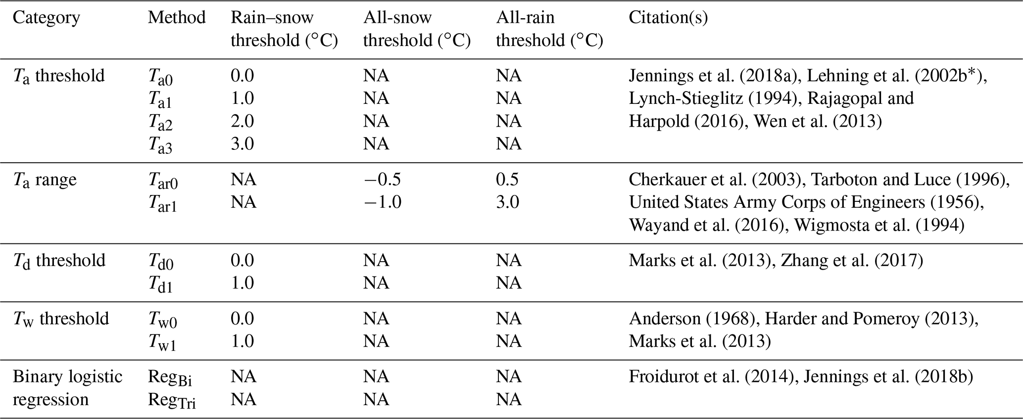
^∗ The SNOWPACK default is a 1.2 ^∘C T_a threshold.

Each of the study sites included RH as part of their meteorological observations, but only the HJA and JD stations had observations of T_d, while no sites had long-term T_w measurements. To keep precipitation phase methods constant across the sites, we calculated T_d (Alduchov and Eskridge, 1996) and T_w (Stull, 2011) as empirical functions of T_a and RH. The empirical formulation tracked observed T_d at JD with an r² of 1.0 and a slight cool bias of −0.3 ^∘C. There were no observations on which to validate the T_w estimates, but Stull (2011) shows biases typically <1.0 ^∘C.

It should be noted that although this work pursues a wide variety of precipitation phase methods, it is not wholly comprehensive. For example, some models fit a sigmoidal curve between two thresholds when assigning precipitation phase in a T_a range (e.g., Fassnacht et al., 2013; Kienzle, 2008; Leavesley et al., 1996). However, we did not include this method because it should produce little variability in annual snowfall fraction relative to the linear T_a ranges if a uniform distribution of T_a and precipitation is assumed within the T_a range. Additionally, models of cloud microphysics are increasingly used to simulate precipitation phase. The wide variety of microphysics schemes available suggests that a critical examination of these methods should be made as well. However, such an analysis is beyond the scope of the current work.

3.3 Evaluating the effect of precipitation phase method selection on snowfall fraction and simulated snow cover evolution

For water years (WY; 1 October of the previous calendar year to 30 September) 2004–2011, we simulated snowpack accumulation and melt at the 11 stations using the SNOWPACK model. Each station had a total of 12 unique model runs corresponding to the different precipitation phase methods. All forcing data and the model setup remained the same across the runs at each site except for the precipitation phase method. For each site and for each of the different precipitation phase methods we quantified the average annual snowfall fraction, peak SWE magnitude, the timing of peak SWE, snowmelt rate, and snow cover duration (Fig. 2). For this work, snowmelt rate is computed as the daily average snowmelt rate between peak SWE timing and the first day where SWE = 0 mm. Snow cover duration is the total number of days when simulated SWE is greater than zero. For each of the sites we present the average simulated quantities noted above as well as the range and relative differences of snow metrics associated with the different precipitation phase methods. In this work, the relative difference is defined as the percentage difference between the maximum and minimum snow metric value (e.g., if T_a0 produced a minimum peak SWE of 200 mm and T_a3 produced a maximum peak SWE of 400 mm, the relative difference would be 100 %). Stations with greater variability in their snow cover evolution metrics were considered to be more sensitive to the choice of precipitation phase method.

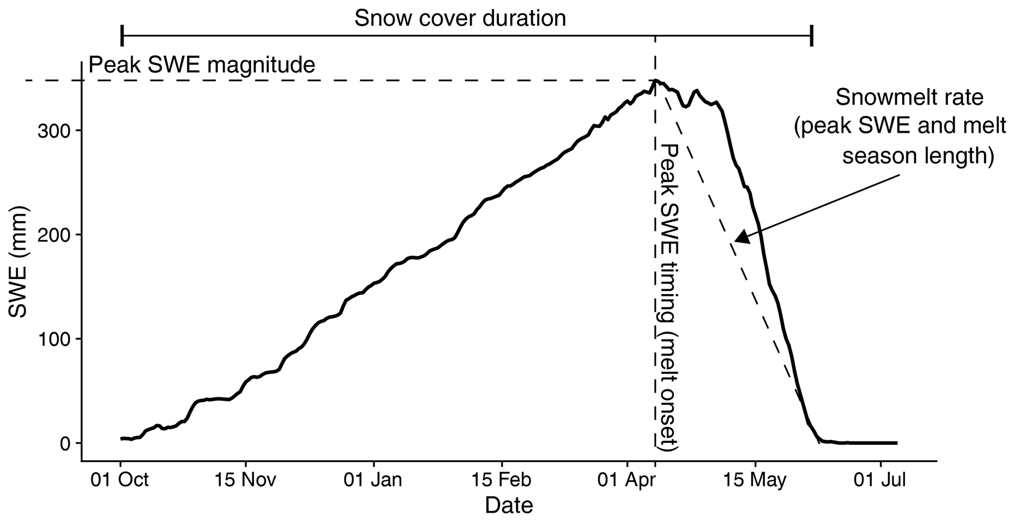
Figure 2 Example plot showing seasonal snow cover evolution, adapted from Trujillo and Molotch (2014).

3.4 Computing the effect of deviating from an optimized rain–snow T_a threshold

We were interested in identifying an optimized rain–snow T_a threshold for our study sites despite a lack of direct precipitation phase observations. We did this through the use of several data sources: (1) the spatially continuous rain–snow T_a threshold map from Jennings et al. (2018b), (2) the observed rain–snow T_a threshold (Jennings et al., 2018b) from the measurement location closest to each study site, (3) changes in observed SWE, and (4) changes in observed snow depth at each site to infer snowfall. For 3 and 4, we used a modified version of the approach of Rajagopal and Harpold (2016) to predict precipitation phase by designating a daily increase of SWE or snow depth as snowfall and a zero change or decrease as rainfall when precipitation was greater than 2.54 mm and SWE or snow depth was greater than 0 mm. We then binned snowfall frequency per 1 ^∘C T_a bin and computed the rain–snow T_a threshold using the hyperbolic tangent equation of Dai (2008). Thresholds from 1, 2, 3, and 4 were then arithmetically averaged and rounded to the nearest integer value to produce an optimized rain–snow T_a threshold for each study site, consistent with the studied threshold values in Table 2. Following this step, we evaluated the effect of deviating by ±1 ^∘C from the optimized threshold by quantifying differences in peak SWE, peak SWE timing, snow cover duration, and snowmelt rate across the selected thresholds.

3.5 Evaluating the relationships between climate and snow cover sensitivity

In addition to quantifying the variability introduced by the different precipitation phase methods, we evaluated the control exerted by daily meteorology and seasonal climate on snow cover evolution sensitivity at our study sites. We first examined how daily average T_a and RH introduced variability into the simulated snowfall fraction. We did this by grouping all daily meteorological conditions in 1 ^∘C T_a bins from −8 to +8 ^∘C and 10 % RH bins from 60 % to 100 % on days with precipitation. We then calculated the standard deviation in the daily snowfall fraction within each bin across all sites and methods. Those results were used to determine the T_a range that produced the greatest standard deviation in the daily snowfall fraction. Next, we computed the proportion of December–May (i.e., winter and spring) precipitation that fell within that T_a range at each site for each simulation year and used that percentage to predict the annual snowfall fraction range with ordinary least-squares regression. Finally, we evaluated how December–May T_a and precipitation produced variability in peak SWE by plotting the peak SWE range as a function of the two meteorological quantities and plotting a predictive surface with a loess function.

4 Results

4.1 Model validation

Figure 3 displays the mean bias and r² values for the different precipitation phase methods relative to observations of SWE and snow depth, aggregated across all stations with a given validation measurement. In terms of mean bias, the binary regression models, Reg_Bi and Reg_Tri, as well as the T_a1 threshold provided the best performance, with average values between 3.1 and 9.1 mm compared to observed SWE and between 4.9 and 14.5 mm compared to observed snow depth. Conversely, the T_a0, T_a2, and T_a3 thresholds and the T_ar0 range provided the worst performance, with T_a2 and T_a3 overpredicting and T_a0 and T_ar0 underpredicting snow accumulation by upwards of 100 mm relative to observed SWE and 200 mm and greater relative to observed snow depth. There was relatively little divergence in r² values across the methods, with differences of only 0.07 and 0.08 between the maximum and minimum average r² values for SWE and snow depth, respectively. The lowest r² values were produced by the T_a0 threshold and T_ar0 range, while T_d1, T_w1, and the higher T_a thresholds produced the highest values.

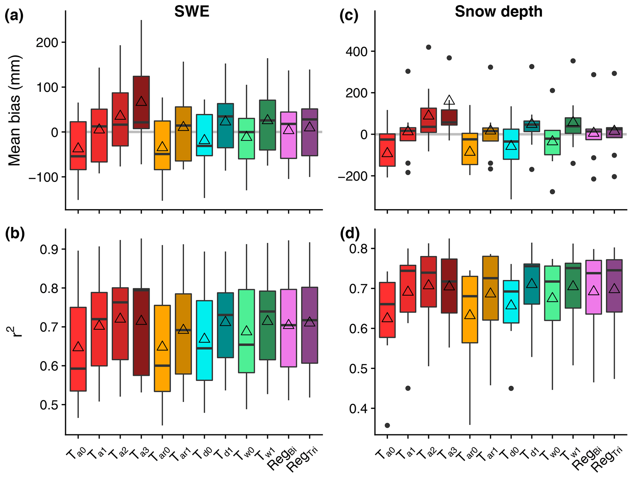
Figure 3 Mean bias (a, c) and r² (b, d) values for the SNOWPACK simulations relative to observed SWE (a, b) and snow depth (c, d). The boxplots show the median, interquartile range, minimum, maximum, and outlying values for each objective function for the different precipitation phase methods at all stations. The open triangles indicate the mean objective function value for that precipitation phase method at all stations.

Figure 4 presents model performance relative to observed SWE and snow depth at the different sites. Mean biases were lowest at the NWT stations and at SSC-UPR relative to SWE observations and at the JD stations and SSC-LWR relative to snow depth observations. Average r² values were between 0.65 and 0.91 for SWE, except at NWT-SDL (0.52) and HJA-VAN (0.51), and 0.61 and 0.79 for snow depth, except at JD-124 (0.46).

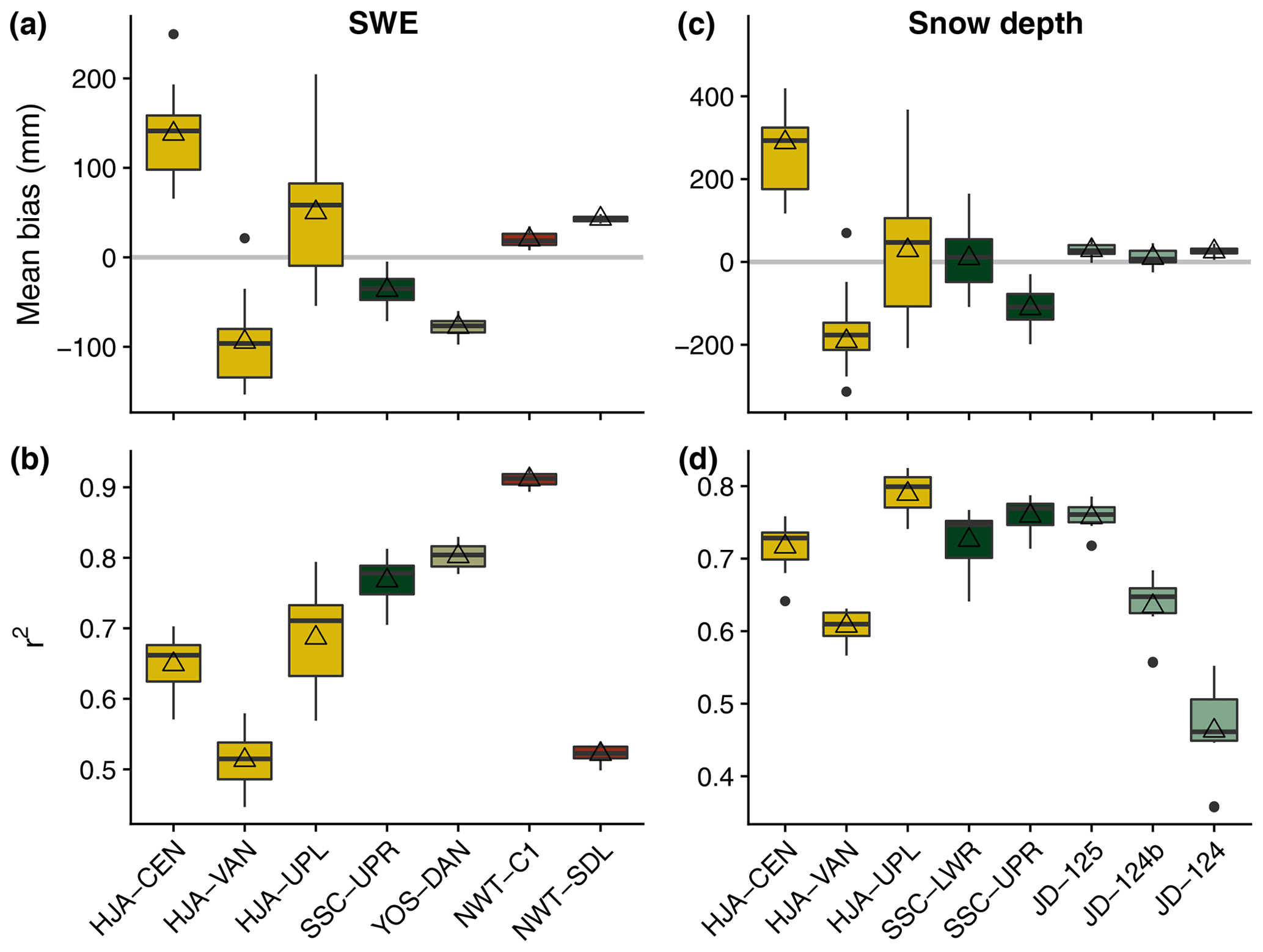
Figure 4 Mean bias (a, c) and r² (b, d) values for the SNOWPACK simulations relative to observed SWE (a, b) and snow depth (c, d). The boxplots show the median, interquartile range, minimum, maximum, and outlying values for each objective function for the different precipitation phase methods at a given station. The open triangles indicate the mean objective function value for all precipitation phase methods at that station. Note: in panel (c) the low mean biases for JD snow depth are due to small snow depth values at the site. Mean relative biases at these stations were 35.4 % (JD-125), 3.8 % (JD-124b), and 35.7 % (JD-124).

4.2 Mean simulated snow cover properties

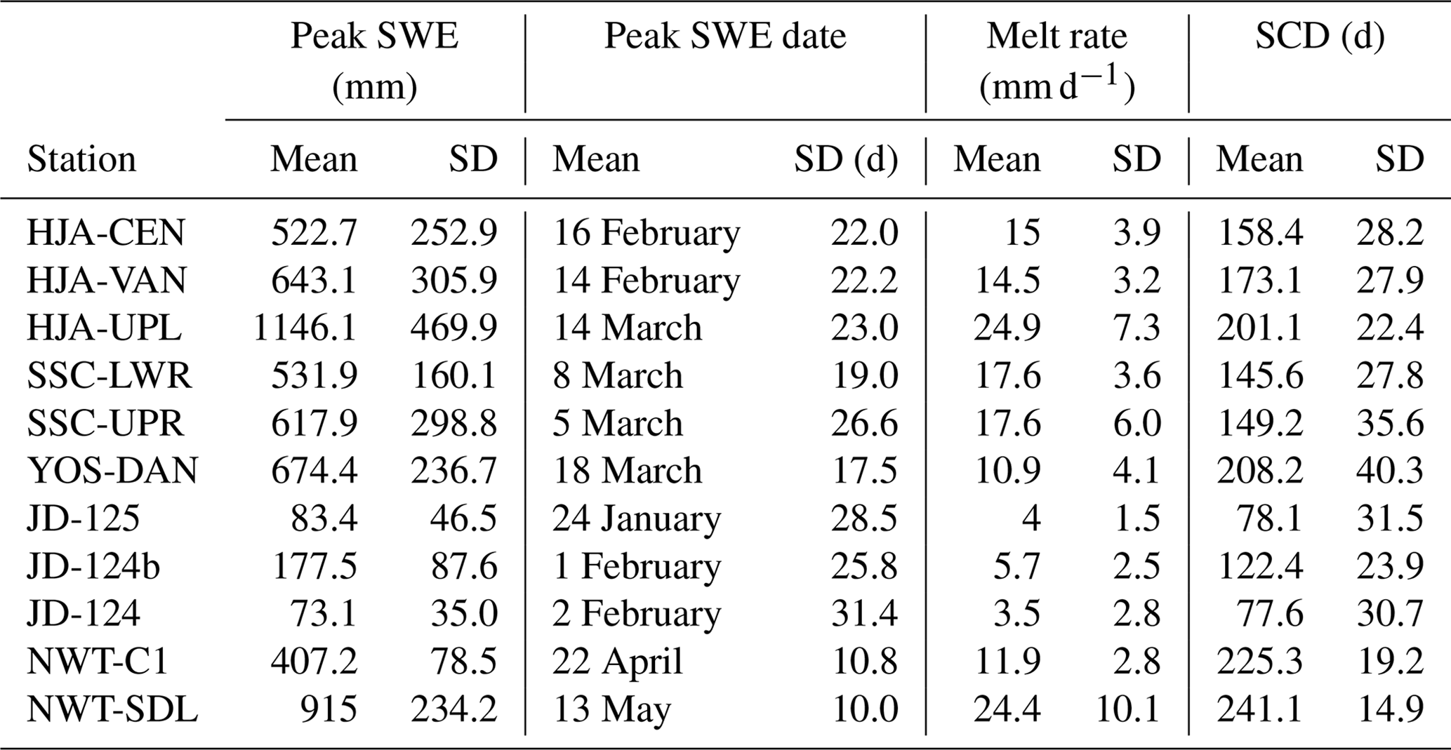
The study locations showed significant differences in simulated snow accumulation and melt. Values presented in Table 3 were computed by taking the mean and standard deviation of the given snow metric using all 12 simulations at each station, where each simulation corresponded to a different precipitation phase method. Mean peak SWE ranged from 73.1 mm at JD-124 to 1146.1 mm at HJA-UPL. The date of peak SWE, or melt onset, also displayed large variability, with values ranging from 24 January at JD-125 to 13 May at NWT-SDL. Melt rates were all greater than 10 mm d⁻¹ during the ablation season except for the JD stations, and the greatest melt rates were simulated at HJA-UPL and NWT-SDL. Snow cover duration was greatest at NWT-SDL at 241.1 d, while snow cover was simulated for less than 3 months, on average, at JD-125 and JD-124.

Table 3 Mean snow cover evolution metrics for the 11 stations. Each mean and standard deviation was calculated across all water years and all precipitation phase methods.

4.3 Effect of precipitation phase method on simulated snowfall fraction

Average annual snowfall fraction (all methods and all years) ranged from 32.3 % at the HJA-CEN station to 92.4 % at the YOS-DAN station (Table 4; Fig. 5). In this case, more strongly seasonal precipitation at YOS-DAN (Table 1) produced a higher annual snowfall fraction than NWT-SDL despite the former station's warmer average T_a. YOS-DAN and NWT-SDL also had the lowest ranges, at 10.1 % and 10.3 %, respectively, suggesting that precipitation phase method selection was less important relative to the other stations. Conversely, the range in the annual snowfall fraction simulated by the different methods was greater than 18 % at all remaining stations, reaching a maximum of 32.3 % at SSC-LWR. For all sites except YOS and NWT, relative differences were greater than 30 %. In some years at HJA, SSC, and JD, the relative difference between the minimum annual snowfall fraction and the maximum exceeded 100 %, meaning that the methods producing the most snow simulated more than double the annual snowfall fraction of those producing the most rainfall. The greatest relative difference in the annual snowfall fraction of 126.9 % was simulated at HJA-CEN, more than 10 times greater than at YOS-DAN and NWT-SDL.

Table 4 Statistics for average annual snowfall fraction computed using the different precipitation phase methods across all simulation years at the 11 study stations. The range was calculated by subtracting the lowest average annual snowfall fraction from the highest average annual snowfall fraction at each station. The relative difference was then computed as the range divided by the minimum and multiplied by 100 %. T_a0 and T_ar0 typically produced the lowest average annual snowfall fractions, while T_a3 and T_d1 led to the highest average annual snowfall fractions.

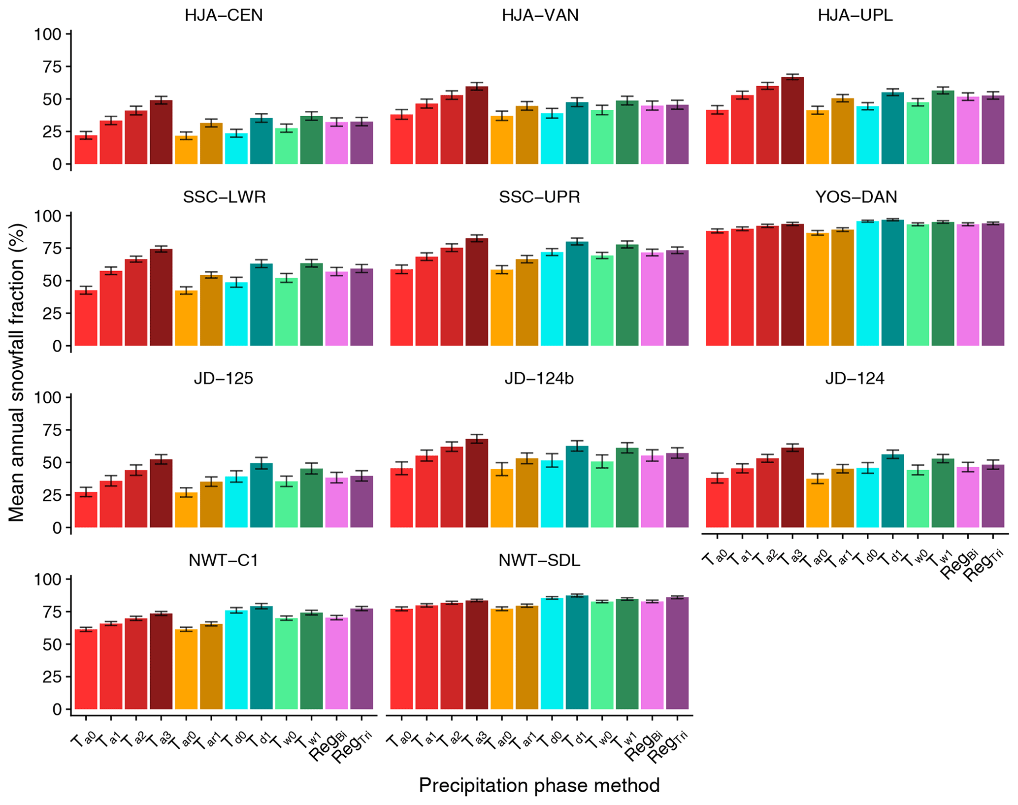
Figure 5 Mean annual snowfall fraction at the 11 study stations for the different precipitation phase methods. The whiskers represent the standard error of annual snowfall fraction for the 8 simulation years. For this plot and all subsequent figures showing the station data, the maritime sites are shown in the top two rows, the intermountain site is in the third row, and the continental site is in the bottom row.

4.4 Effect of precipitation phase method on simulated snow accumulation and melt

There were marked differences between the stations in terms of the effect that precipitation phase method choice had on seasonal snow cover evolution. Figure 6 presents the simulated mean daily SWE of all simulation years at the study stations along with the difference between the minimum and maximum mean daily SWE produced by the precipitation phase methods. At HJA, SSC, and JD, differences increased throughout the accumulation period, reaching a maximum after peak SWE during the snowmelt season. At NWT and YOS, the differences were typically negligible throughout the accumulation season, as cold winter and early spring temperatures produced little divergence in the amount of snowfall versus rainfall simulated by the different methods. At these stations, differences in the mean daily SWE produced by the precipitation phase methods did not appear until approximately the date of peak SWE. Mean daily SWE differences were always less than 90 mm at NWT and YOS, while they sometimes exceeded 200 mm at HJA and SSC. Differences were typically small in magnitude at JD but were proportionally large due to low mean daily SWE values.

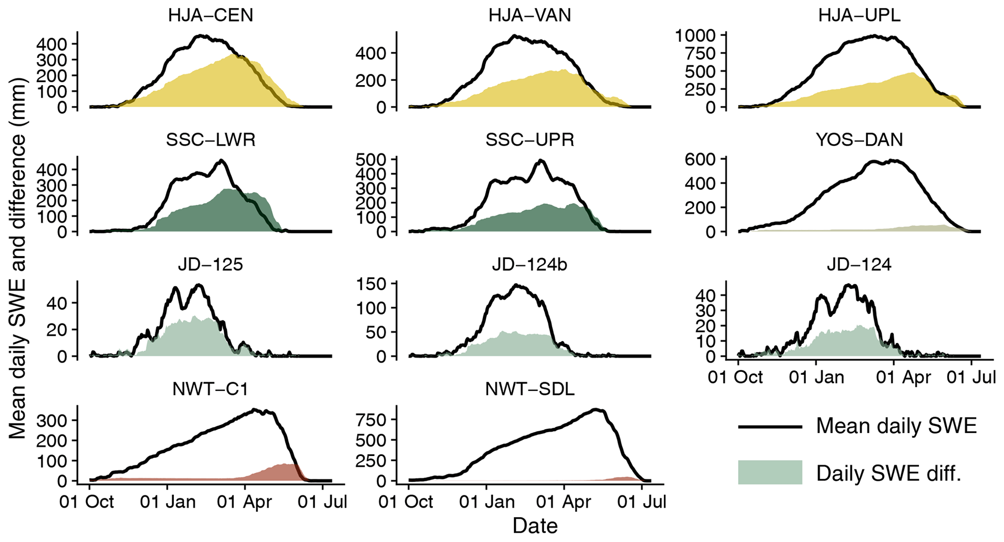
Figure 6 Mean daily simulated SWE (solid black line) and the difference between maximum and minimum mean daily SWE (shading) at the study stations. The mean daily SWE was computed by averaging the simulated SWE on each day for all precipitation phase methods across the simulation years. The difference was calculated by subtracting the minimum mean daily SWE from the maximum mean daily SWE produced by the different precipitation phase methods (mean daily SWE plots broken out by precipitation phase method can be viewed in Figs. S1–S11). The T_a0 and T_ar0 methods typically produced the minimum mean daily SWE, while T_a3 and T_d1 produced the maximum.

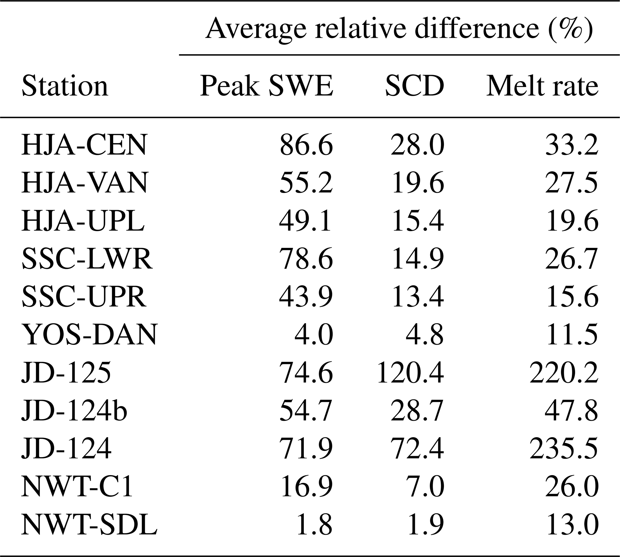
Breaking down the analysis to the individual snow cover evolution metrics reveals more differences in the sensitivity of the sites to precipitation phase method selection (Fig. 7). In terms of the peak SWE range, the HJA and SSC stations were most sensitive, with average ranges all greater than 200 mm, exceeding 400 mm in some years (Fig. 7a). Conversely, YOS and NWT were relatively insensitive, as their average ranges were all less than 65 mm. The largest annual range in peak SWE at the NWT and YOS stations was just 90.8 mm at NWT-C1, which was considerably less than the maximum peak SWE range of 592.5 mm simulated at HJA-UPL. Although the JD stations showed little sensitivity in terms of range with average annual peak SWE differences being less than 55 mm, they expressed significant sensitivity when looking at relative differences (Table 5) due to their low mean annual peak SWE (Table 3). Thus, percentage-wise, JD was as sensitive as the two warm maritime sites to the selection of a precipitation phase method. At JD, HJA, and SSC it was common for the relative difference between minimum and maximum modeled peak SWE to be well above 50 %, meaning that a significant proportion of water was simulated to have infiltrated or run off using one precipitation phase method versus being stored in the snowpack using another method. This is in stark contrast to the 4.0 % and 1.8 % relative differences at YOS-DAN and NWT-SDL.

Figure 7 The annual range in simulated peak SWE (a), peak SWE date (b), snow cover duration (c), and melt rate (d) due to precipitation phase method selection at the study stations.

Table 5 Average relative differences in annual peak SWE, snow cover duration, and melt rate at the 11 stations. Relative differences were not computed for peak SWE date because the relative difference value would change depending on if day of year or day of water year were used in the calculation.

JD and HJA were also sensitive to precipitation phase method selection in terms of peak SWE date (Fig. 7b), with four of the six stations having average ranges greater than 2 weeks. In some simulation years, peak SWE date ranges exceeded 1 month at HJA, JD, and SSC. We found that the greatest differences in peak SWE dates were generally simulated on years with low or transient snow cover. In these cases, late-season precipitation was simulated as rain by the low T_a thresholds and snow by the high T_a thresholds, meaning that an early SWE maximum was recorded as the peak in the former case and a late SWE maximum in the latter case. Compared to the other stations, peak SWE date ranges were generally small at NWT-SDL and YOS-DAN, with an average range of just 0.8 d at the former and 2.5 d at the latter.

Similar sensitivities were simulated for snow cover duration (Fig. 7c), with the warm maritime sites and JD being the most impacted by precipitation phase method choice. JD-125 had the greatest average range in annual snow cover duration at 42.0 d, and all other ranges at JD and HJA were greater than 26.8 d. SSC-LWR and SSC-UPR expressed slightly lower average ranges at 20.9 and 18.1 d, respectively. NWT-C1 approached the sensitivity of the warmer stations, while NWT-SDL and YOS-DAN were again the least sensitive. Relative differences were greatest at JD (Table 5) because simulated snow cover was typically of a shorter duration compared to the other sites (Table 3). The average relative difference at JD-125 of 120.4 % meant that snow cover simulated using the T_a3 threshold lasted twice as long as snow cover using the T_a0 threshold. Notably, there was an order of magnitude of difference between JD, HJA, and SSC and YOS and NWT, with average relative differences in snow cover duration being greater than 10 % at the former three sites and less than 10 % at the latter two.

Differences among the stations were relatively low for melt rate (Fig. 7d), with the interquartile ranges generally showing some degree of overlap. JD stations had the greatest sensitivity in terms of relative differences (Table 5) due to their low mean annual melt rates, which were an order of magnitude lower than those simulated at the other sites (Table 3). Overall, the melt rate at YOS-DAN was the least affected by precipitation phase method selection in terms of range and relative difference. It should be noted here again that the forcing data were kept constant for the different modeling scenarios – only the precipitation phase methods were varied. Thus, any changes to the melt rate were caused by shifts in snowmelt timing and by the hydrologic and energy balance impacts of rain versus snow.

To close this section, it is useful to visualize what these differences look like in terms of annual snow cover evolution. Figure 8 shows examples of large ranges in peak SWE (Fig. 8a), peak SWE date and melt rate (Fig. 8b), and snow cover duration (Fig. 8c), while Fig. 8d exemplifies a year with little simulated divergence in the snow cover metrics. For peak SWE, it is evident that differences in snow accumulation begin with the first snowfall, and the SWE simulated by the various precipitation phase methods continues to diverge throughout the accumulation season (Fig. 8a). In Fig. 8b, simulated SWE is fairly consistent and tracks observed SWE early in the accumulation season before diverging at the onset of winter snowmelt. T_a2 and T_a3 produce a late peak SWE on 7 April, with melt rates greater than 24 mm d⁻¹, while all other methods predict peak SWE to occur 52 to 53 d earlier, with slower melt rates between 15.5 and 16.3 mm d⁻¹. In terms of snow cover duration, years with transient snow tended to be most sensitive, as Fig. 8c illustrates. Modeled snow depth generally follows the observed pattern of accumulation and melt, but the methods diverge in terms of how often and for how long they reach 0 mm. Finally, there is little divergence in simulated SWE throughout the entire accumulation season at NWT-C1, with small differences arising only after the date of peak SWE (Fig. 8d).

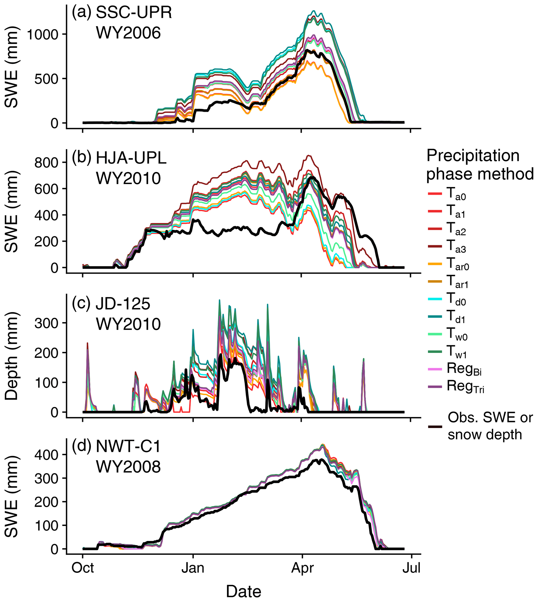
Figure 8 Example simulation years from a selection of stations showing pronounced differences in peak SWE magnitude (a), peak SWE date and snowmelt rate (b), and snow cover duration (c). Panel (d) exemplifies a site and year with little divergence in the studied snowpack metrics. In all panels simulated SWE and snow depth are represented by colored lines for the different methods, while observed SWE and snow depth are shown in black.

4.5 The effect of deviating from an optimized rain–snow T_a threshold

Using the data outlined in Sect. 3.4, we identified optimized rain–snow T_a thresholds of 1.0 ^∘C for HJA and SSC, 2.0 ^∘C for YOS-DAN and JD, and 3.0 ^∘C for NWT (for all snowfall frequency curves and threshold values, please see Figs. S12 and S13 and Table S2). Again, we rounded to the nearest integer value to be consistent with the other T_a thresholds studied in this work. Consistent with our findings in Sect. 4.4, the warm maritime HJA and SSC stations were profoundly affected by deviations from the optimized threshold (Fig. 9). Differences at these sites produced by deviating by only ±1 ^∘C from the optimized thresholds range between 141 and 403 mm for peak SWE, 1 and 16 d for peak SWE day of water year (DOWY), and 9 and 29 d for snow cover duration (SCD). Compare this to 1 to 10 mm for peak SWE, 0 to 1 d for peak SWE DOWY, and 1 to 5 d for SCD at the YOS and NWT stations. The consistent story is again that threshold choice makes a much larger impact at a warm site relative to a cold one.

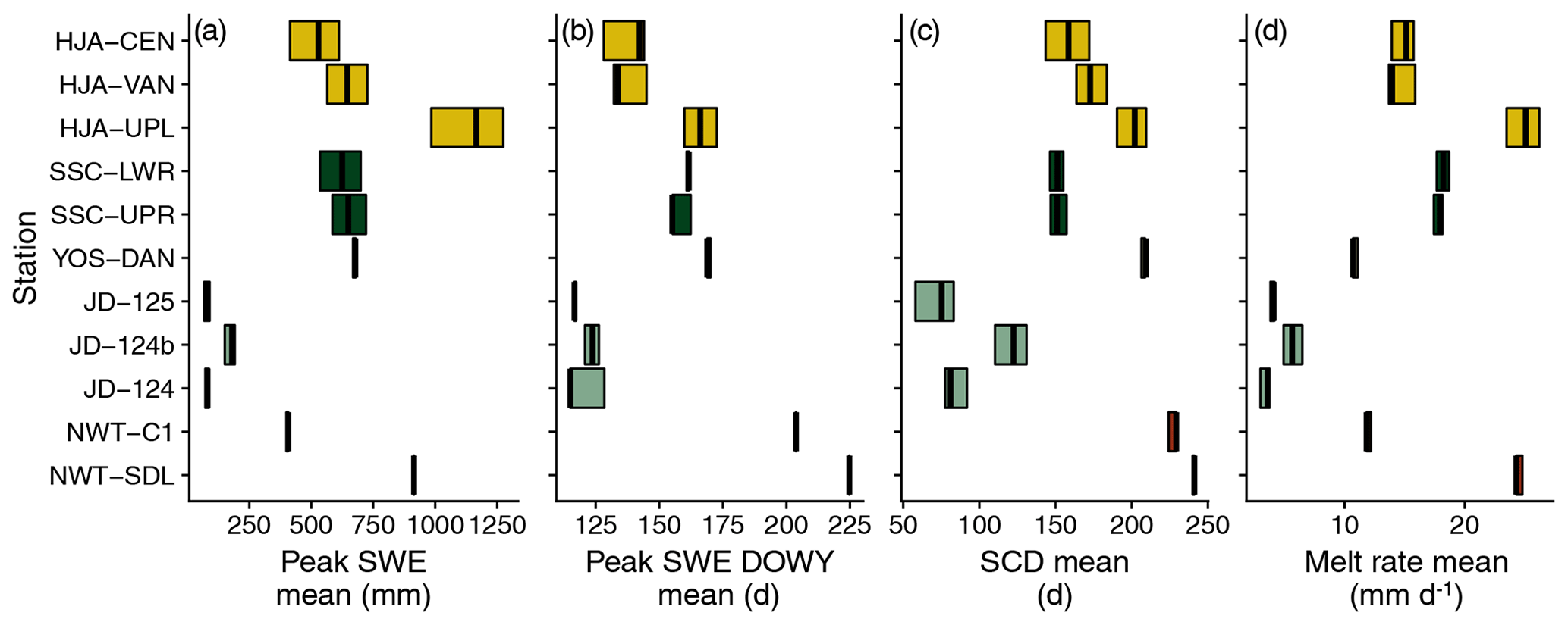
Figure 9 Mean peak SWE (a), peak SWE day of water year (DOWY; b), snow cover duration (SCD; c), and melt rate (d) for the different stations. The width of the bar in each plot represents the spread between the mean snow cover metric value when the model was run with the optimized threshold plus 1 ^∘C and the optimized threshold minus 1 ^∘C. The center line represents the snow cover metric value when the model was run with the optimized threshold. Note: at NWT, only −1 ^∘C from the optimized value of 3 ^∘C was evaluated because we did not include a 4 ^∘C threshold in this work.

4.6 Climatic controls on precipitation phase method sensitivity

In general, the daily snowfall fraction standard deviation was greatest at daily T_a values between 0 and 4 ^∘C (Fig. 10a). RH provided a secondary control, with greater daily snowfall fraction variability at lower RH values (Fig. 10b). Overall, the largest standard deviations in snowfall fraction were simulated at a daily RH less than 80 % and T_a between 1 and 3 ^∘C. However, it should be noted that 75.2 % of all precipitation recorded at the study stations occurred in the 90 %–100 % RH bin. Therefore, although daily snowfall fraction standard deviations were highest at lower RH values, the majority of the variability in snowfall fraction was an effect of T_a. In this context, the percentage of December–May precipitation that fell within the 0–4 ^∘C T_a range explained 80.1 % of the variance in the annual snowfall fraction range across the study sites (Fig. 11).

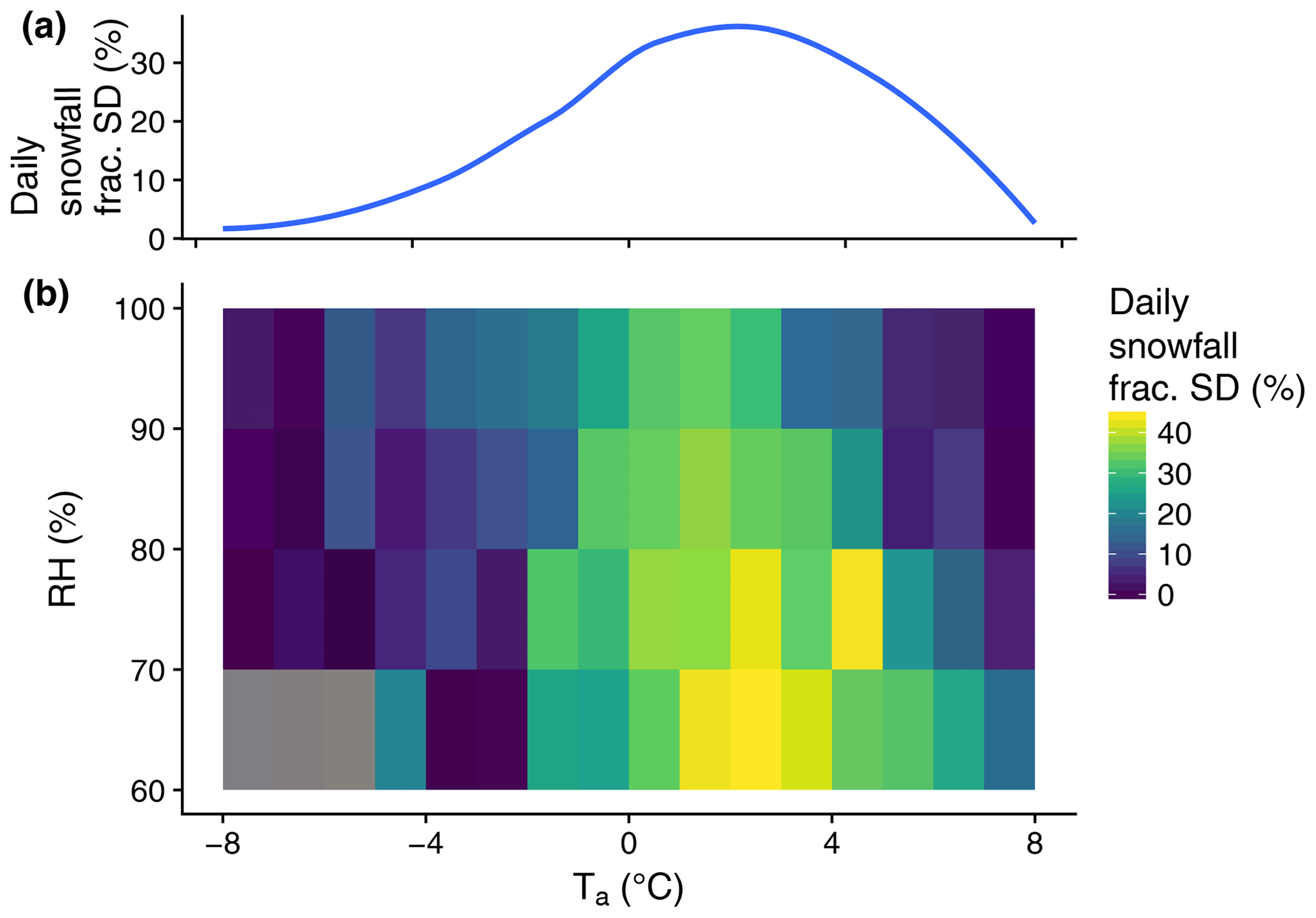
Figure 10 The standard deviation of daily snowfall fraction as a function of T_a (a) and as a function of T_a and RH (b). We binned the meteorological quantities within the ranges shown and calculated the standard deviation of snowfall fraction per T_a bin (a) and T_a ∕ RH bin (b) using simulated precipitation phase from all stations and all methods.

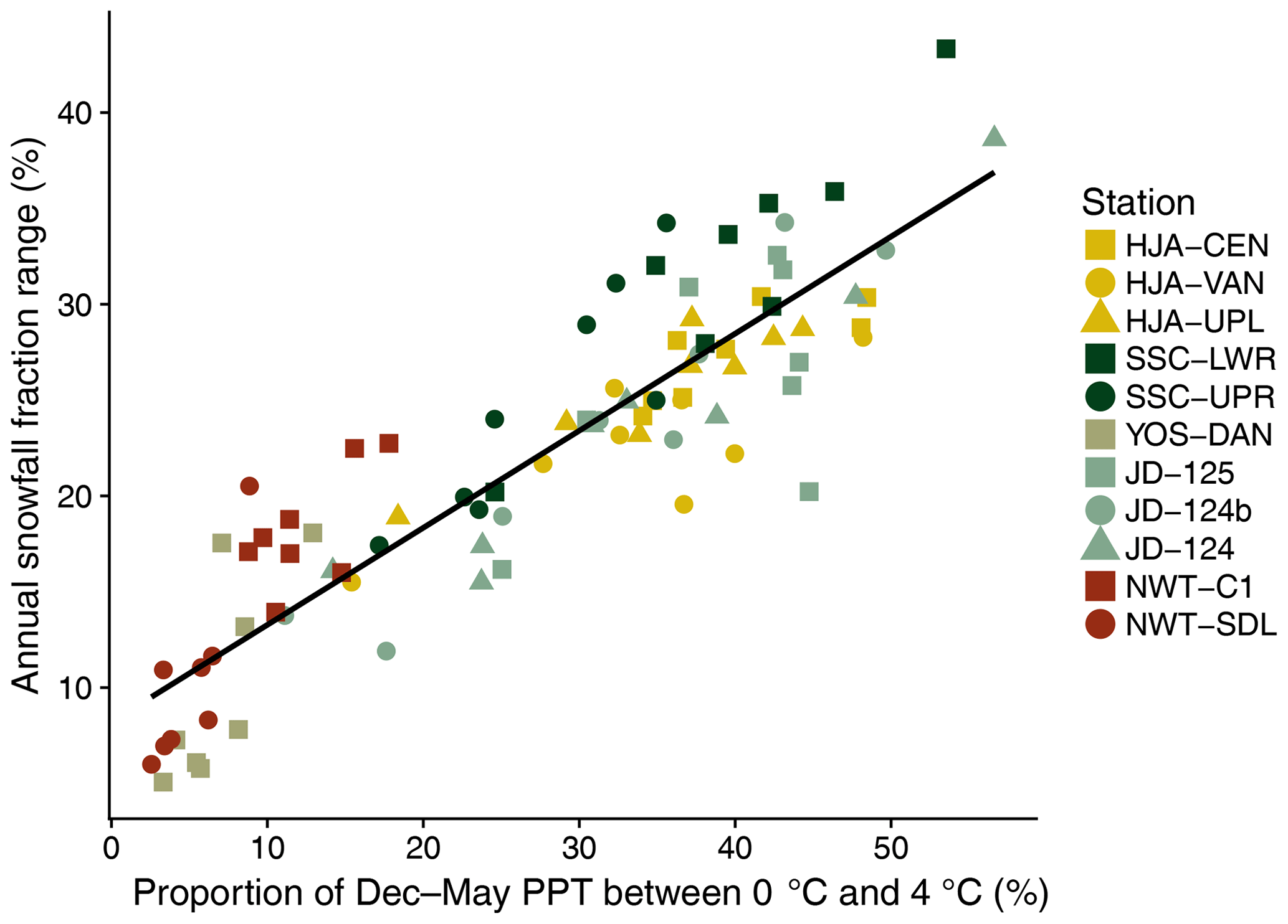
Figure 11 Range in annual snowfall fraction as predicted by the proportion of December–May PPT falling between 0 and 4 ^∘C. Each point represents one simulation year at a station identified by the color and shape. The black line of best fit was calculated using ordinary least-squares regression (r²=0.80; p value <0.0001).

We next evaluated how sensitivity in peak SWE was related to seasonal climate. In this case, warmer T_a and increased PPT were both associated with greater ranges in the peak SWE simulated by the different precipitation phase methods (Fig. 12). This meant that the maritime sites HJA and SSC had the greatest sensitivity to the precipitation phase method due to their relatively warm T_a and high PPT values. Conversely, moderate PPT values and lower T_a led to minimal sensitivity at the cold continental NWT stations and the cold maritime YOS-DAN station. Again, the effect of T_a on sensitivity was manifest in the data. In high snowfall years at NWT-SDL, December–May PPT approached that of the low December–May PPT years at HJA and SSC. However, despite the increased PPT at NWT-SDL, the range in peak SWE predicted by the different precipitation phase methods remained low.

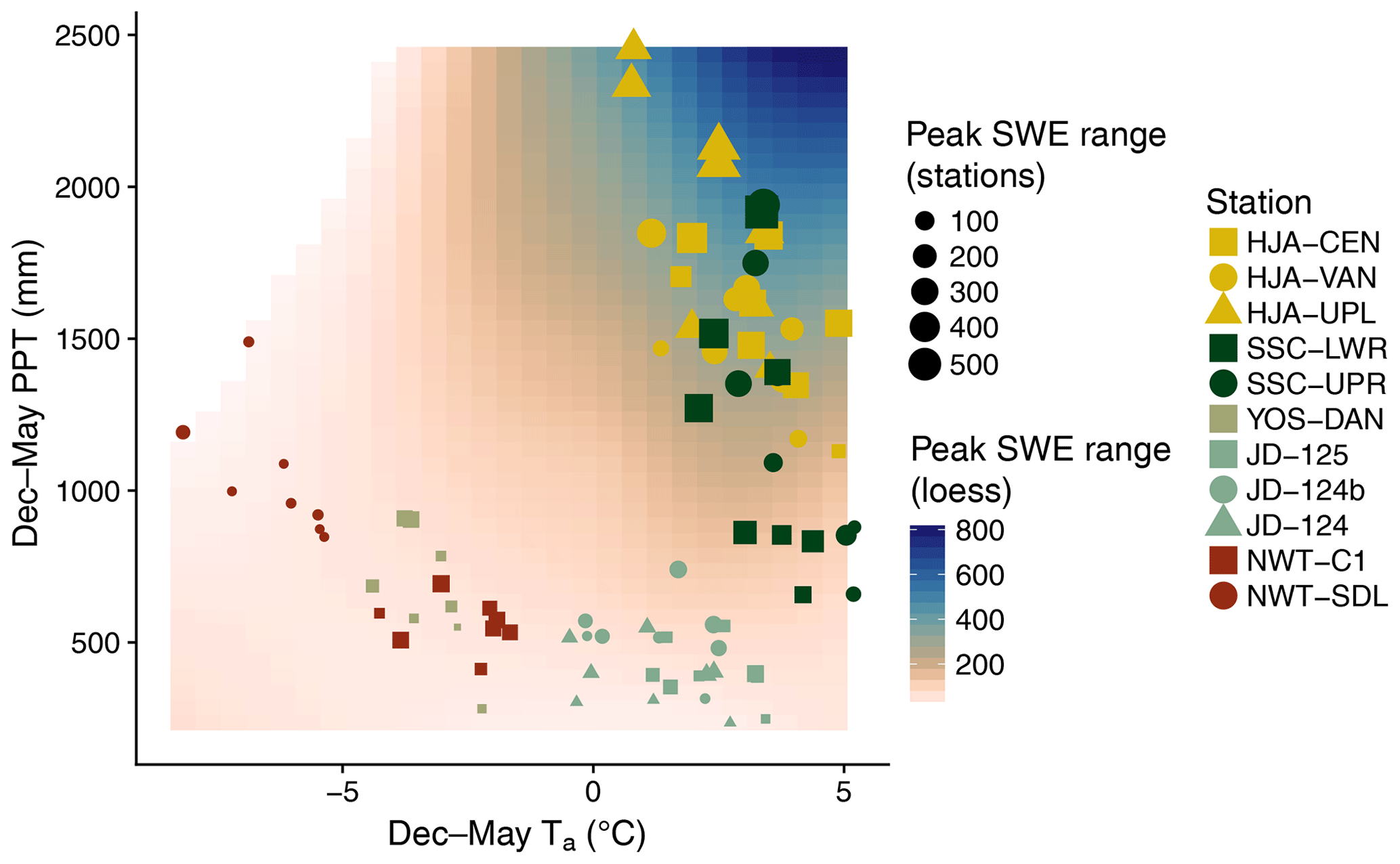
Figure 12 Range in annual peak SWE as simulated by the different precipitation phase methods at the 11 study stations. Each point represents one simulation year at a given station, and larger points correspond to larger differences in maximum minus minimum peak SWE. The background shading corresponds to ranges in peak SWE predicted by a loess function fit to the station data.

5 Discussion

5.1 A best precipitation phase method?

In this work we showed that the selection of a precipitation phase method produces varying degrees of variability in modeled snow accumulation and melt at our study stations. The different methods also expressed variable performance relative to observations of SWE and snow depth, with the binary regression models, Reg_Bi and Reg_Tri, as well as the T_a1 threshold producing the lowest biases (Fig. 3). Previous observational work has shown that, in general, methods incorporating humidity information outperform T_a-only methods when it comes to predicting precipitation phase (Harder and Pomeroy, 2013; Jennings et al., 2018b; Marks et al., 2013; Ye et al., 2013). The Reg_Bi method, which predicts phase as a function of T_a and RH, exceeded all other methods in partitioning rain and snow in a Northern Hemisphere precipitation phase method comparison (Jennings et al., 2018b). Our study showed that Reg_Bi also typically produced simulations of SWE and snow depth that had low biases relative to observations (Fig. 3) and led to snow cover evolution metrics that were neither extremely high nor low compared to the other methods examined in this work. This finding is complemented by the performance of other humidity-based metrics, which produced average SWE and snow depth biases between −19.2 and 25.1 and −58.3 and 56.7 mm, respectively.

This is in contrast to the T_a thresholds and ranges, which produced the largest magnitude biases. Notably, the four worst performers were the T_a0, T_ar0, T_a2, and T_a3 methods, with the former two underpredicting snow accumulation and the latter two overpredicting it. Across our study sites, the only T_a methods that performed well relative to observations were the T_a1 threshold and T_ar1 range. These modeling results confirm again that including humidity information, whether it is in the form of a binary logistic regression model, T_w, or T_d, offers advantages over a T_a-only method. It is important to note again that we chose methods that covered the range in rain–snow partitioning T_a values across our study domain or that included humidity information. The only methods not falling into this category were T_a0 and T_ar0, which were chosen because they are still employed as default methods in some models and studies. Although there are some small geographic regions where such a threshold or range may be appropriate (Jennings et al., 2018b), they are unsuitable for many locations and should not be used for large-scale studies.

In the course of this work we found negligible differences between T_a0 and T_r0 as well as between T_a1 and T_r1 in terms of annual snowfall fraction (Fig. 5) and model performance (Fig. 3). This suggests that the ranges and the mixed-phase precipitation they produced provided little further information on precipitation phase at the hourly model timescale relative to the thresholds. However, it should be noted there are relatively few quantitative data on the frequency and solid–liquid proportions of mixed-phase events (e.g., Yuter et al., 2006). Work from the Turin region of Italy showed that mixed-phase events are relatively few compared to all-rain and all-snow events (Avanzi et al., 2014), while research in a maritime climate indicated that mixed-phase events can be quite frequent (Wayand et al., 2016). Future work would therefore benefit from further explorations of the frequency of mixed-phase events and model representations thereof at multiple timescales.

Despite the analyses presented in this work, it is important to note that uncertainties in forcing data, model structure and parameters, and a lack of precipitation phase observations prevent this research from being able to unequivocally identify a “best” precipitation phase method for snow modeling. However, as noted above, including humidity information improves the prediction of precipitation phase relative to observations and generally increases model performance. Our primary aim in this research was to quantify how snow simulations were affected by the choice of precipitation phase method across a climatic gradient. We did not create optimized model setups at each site but rather kept the model setup consistent in order to compare the sensitivity of phase partitioning without introducing other uncertainties. Thus, the low r² and higher bias values at HJA-VAN, NWT-SDL, and JD-124 (Fig. 4) could likely be improved with model tuning, but we did not pursue such an approach. Additionally, we showed in Sect. 4.5 that deviating from an optimized T_a rain–snow threshold by ±1 ^∘C had a much larger effect on simulated snow accumulation and melt at HJA and SSC than YOS and NWT. Such a finding indicates that finding an optimal threshold is much more important in areas with winter T_a near freezing.

5.2 Assumptions and limitations

Snow modeling studies are hindered by inherent uncertainties in model structure (Essery et al., 2013; Etchevers et al., 2004; Rutter et al., 2009; Slater et al., 2001) and forcing data (Lapo et al., 2015; Raleigh et al., 2015, 2016). While the research presented herein shows that the precipitation phase method should be considered another critical component of model uncertainty, our work was also likely affected by the aforementioned issues in structure and forcing data which can be seen in the variability in model performance at the different sites (Fig. 4). In this work, we used the well-validated, physics-based SNOWPACK model, but past research has shown that there is no best snow model and that model performance varies both within and across study sites (e.g., Rutter et al., 2009). Given this variable performance and differences in snow model structure and physics, it is possible that some models may be more or less sensitive to the choice of a precipitation phase method. Our use of a single model may overestimate or underestimate the sensitivity of snow accumulation and melt to precipitation phase method selection. Future research should therefore focus on how model choice affects the sensitivity of simulated snow cover evolution to the precipitation phase method.

In addition to the uncertainties introduced by the SNOWPACK model, we used empirical methods to estimate T_d and T_w, which could affect rain–snow partitioning. We were satisfied with the performance of the T_d method, as it strongly matched T_d observations from JD (Sect. 3.2). However, there were no observations of T_w on which to validate the Stull (2011) method, which was optimized for standard surface pressure and for a range of T_a and RH values. The figures in Stull (2011) show that pressure-induced uncertainty in T_w is generally less than 1 ^∘C when RH >50 %. Additionally, the total percentage of precipitation observations falling within the Stull (2011) T_a and RH ranges was between 94.3 % and 100 % at our stations. Thus, we expect only marginal uncertainty to be introduced by the empirical methods. However, precipitation phase and hydrometeor temperature are strongly related to T_w (Harder and Pomeroy, 2013), suggesting that there should be enhanced monitoring of T_w at research sites.

Furthermore, our research only examined methods that partition precipitation phase using surface meteorological quantities such as T_a, RH, and P_s. Atmospheric and climate models can also be used for hydroclimatic simulations either through direct coupling in earth system models or as forcing data for land surface models. Many such models employ microphysics schemes to assign and track precipitation phase from the formation of a hydrometeor, through various atmospheric layers, to the land surface. For example, the Weather Research and Forecasting (WRF) model (Skamarock et al., 2005) has been used to simulate snow cover accumulation and ablation over large study domains in the western United States when coupled to a land surface model (Ikeda et al., 2010; Musselman et al., 2017a; Rasmussen et al., 2011). WRF has also been used to model the elevation of the rain–snow transition line in order to evaluate which basin areas are receiving solid or liquid precipitation during storm events (Minder et al., 2011). In addition, work from the fifth phase of the Coupled Model Intercomparison Project (CMIP5) has shown that climate models produce different snowfall fractions due to variations in both climate and the precipitation phase method (Krasting et al., 2013). In CMIP5, some models utilize microphysics schemes, while others assign precipitation phase at the land surface using methods similar to the ones presented in this work. Therefore, understanding and quantifying the sensitivity of model output due to precipitation phase method selection are important for both hydrologic and climate modeling studies.

5.3 Physical mechanisms controlling sensitivity to phase method

The warm maritime sites HJA and SSC expressed the largest peak SWE ranges from precipitation phase method selection (Fig. 7). These ranges were typically larger than 200 mm and sometimes exceeded 400 mm with relative differences usually greater than 50 %, indicating large uncertainty in snowpack water storage. Additionally, peak SWE date ranges typically exceeded 2 weeks at these stations, meaning that the timing of snowmelt onset was also affected by the precipitation phase method. These large variations in snow cover evolution were likely due to the combined effect of reduced frozen mass entering the snowpack and subsequent changes to the snowpack energy balance. For the former, both HJA and SSC had high proportions of precipitation falling between 0 and 4 ^∘C (Fig. 11), which led to wide ranges in the annual snowfall fraction (Table 4). The methods producing lower annual snowfall fractions (e.g., T_a0 and T_ar0) generally corresponded to reduced snow cover duration simply because there was less frozen mass to melt. In other words, the energy required to melt the entire snowpack was reduced relative to the methods producing higher snowfall fractions, and the snowpack could be melted over a shorter time period.

Compounding the response of the warm maritime sites is the fact that snow and rain have different fates when they enter a snowpack, with resultant effects on the snowpack energy budget. Snowfall can increase snowpack cold content (Jennings et al., 2018a), refresh surface albedo (Clow et al., 2016; Molotch et al., 2004; Molotch and Bales, 2006; Painter et al., 2012; United States Army Corps of Engineers, 1956), and provide dry pore space that must reach field capacity with liquid water before runoff can begin (Bengtsson, 1982; Seligman et al., 2014). Rainfall, conversely, can advect heat to the snowpack (Marks et al., 1998), infiltrate and run off (Harr, 1981, 1986), or be refrozen in the snowpack if there is cold content to be satisfied. In this context, the precipitation phase methods that produced more rainfall likely affected snow cover evolution not just through reduced frozen mass but also through changes to the snowpack energy budget. Further observational and modeling research is warranted to evaluate how rain versus snow affects snowpack energetics.

5.4 Why precipitation phase matters to climate warming simulations

The shift from snow to rain in cold and temperate regions across the globe is expected to continue with further warming. Future air temperature increases will likely produce reduced snowfall fractions (Klos et al., 2014; Lute et al., 2015; Safeeq et al., 2015), lower peak SWE values (Adam et al., 2009), earlier snowmelt onset (Stewart et al., 2004), slower snowmelt rates (Musselman et al., 2017a), and changes to the intensity and location of rain-on-snow events (Musselman et al., 2018). These warming-driven changes will impact both water resource availability (Barnett et al., 2008) and land surface albedo (Déry and Brown, 2007). Most at risk of reductions in the snowfall fraction and snow accumulation are areas with winter T_a near 0 ^∘C (Nolin and Daly, 2006). Concerningly, our work shows that it is precisely these areas that have the greatest modeled snow cover accumulation and melt sensitivity to precipitation phase method selection. Compounding the problem is the fact that all precipitation phase methods exhibit downgraded performance relative to observations between 0 ^∘C and 4 ^∘C (Ding et al., 2014; Jennings et al., 2018b).

Harpold et al. (2017c) showed that future changes to snowfall fraction are moderated or exacerbated by the choice of a precipitation phase method, depending on the area's relative humidity. However, how this uncertainty affects the conclusion of climate change predictions is typically not discussed. In the context of the work presented herein, there should be a focus applied to areas where the baseline variability in peak SWE, snowmelt onset, and snow cover duration due to precipitation phase method approaches or exceeds the simulated change in the associated snowpack properties with warming. In warm maritime climates, research has shown that peak SWE may decrease by upwards of several hundred millimeters as warming continues (e.g., Cooper et al., 2016; Leung et al., 2004; Minder, 2010; Musselman et al., 2017b), which is near the range of peak SWE sensitivity values reported in this work. Precipitation phase method selection is also likely to impact simulations of future warm snow droughts, where anomalously warm winters are associated with low peak SWE (Harpold et al., 2017a). In addition, snow cover duration variability due to precipitation phase method selection in earth system models may affect simulations of the snow–albedo feedback, which is the amplification of surface warming due to reduced snow cover (Hall, 2004; Hall and Qu, 2006). As climate warming shifts new areas towards the winter and spring average T_a values (0–4 ^∘C) that lead to the greatest uncertainty in rain–snow partitioning, our research suggests that uncertainty in future hydroclimatic states will be exacerbated by precipitation phase method selection.

6 Conclusion

In this work we simulated seasonal snow cover evolution using the SNOWPACK model forced with different permutations of five precipitation phase methods at 11 study stations spanning a climatic gradient from warm maritime to cold continental. We found that the choice of a precipitation phase method affected model performance and introduced significant variability into simulated snow accumulation and melt. Overall, the binary logistic regression models produced the lowest mean biases, while high and low air temperature thresholds tended to overpredict and underpredict snow accumulation, respectively. Warm maritime sites were the most sensitive to method selection, with relative differences in the annual snowfall fraction near and above 100 % and ranges in peak SWE typically greater than 200 mm, exceeding 400 mm in certain years. At these sites the different methods produced ranges in snowmelt timing and snow cover duration that were generally longer than 2 and 3 weeks, respectively. Conversely, the YOS-DAN and NWT-SDL stations exhibited the lowest sensitivity to precipitation phase method selection, with relative differences in the annual snowfall fraction between 11.6 % and 13.4 %. Peak SWE ranges were typically less than 30 mm for these two stations, while average snowmelt onset date ranges were only 0.8 and 2.5 d at YOS-DAN and NWT-SDL, respectively. In contrast to the marked differences in peak SWE, melt onset, and snow cover duration between the warm and cold stations, ranges in the snowmelt rate exhibited a small relationship to seasonal climate. Additionally, we found that deviating by ±1 ^∘C from an optimized T_a rain–snow threshold had a relatively small effect on simulated snow cover evolution at NWT and YOS compared to the larger sensitivity at HJA, SSC, and JD.

The spatially variable sensitivity of snow cover evolution was primarily a result of climatic differences between the stations. Increased December–May T_a and PPT were associated with greater peak SWE ranges across the different precipitation phase methods. This meant that the maritime sites HJA and SSC, with significant winter and spring PPT, were most affected by precipitation phase method selection. Overall, we found stations with a high proportion of December–May PPT falling at T_a between 0 and 4 ^∘C to be more sensitive than those with less PPT in that T_a range. This is troublesome, considering that climate warming is expected to push new areas in the seasonal snow zone towards winter T_a near 0 ^∘C and above. It is therefore critical that future work examine the relationship between the effect of warming on snow cover evolution and the model variability that results from precipitation phase partitioning uncertainty, particularly in areas undergoing a snow-to-rain transition.