the Creative Commons Attribution 4.0 License.
the Creative Commons Attribution 4.0 License.
 | 15 Aug 2019
Uncertainty quantification of floodplain friction in hydrodynamic models
Guilherme Luiz Dalledonne
Rebekka Kopmann
Thomas Brudy-Zippelius
This study proposes a framework to estimate the uncertainty of hydrodynamic models on floodplains. The traditional floodplain resistance formula of Pasche (1984) (based on Lindner, 1982) used for river modelling as well as the approaches of Baptist et al. (2007), Järvelä (2004), and Battiato and Rubol (2014) was considered for carrying out an uncertainty quantification (UQ). The analysis was performed by means of three different methods: traditional Monte Carlo (MC), first-order second-moment (FOSM) and metamodelling. Using a two-dimensional hydrodynamic model, a 10 km reach of the River Rhine was simulated. The model was calibrated with water level measurements under steady flow conditions and then the analysis was carried out based on flow velocity results. The compared floodplain friction formulae produced qualitatively similar results, in which uncertainties in flow velocity were most significant on the floodplains. Among the tested resistance formulae the approach from Järvelä (2004) presented on average the smallest prediction intervals, i.e. the smallest variance. It is important to keep in mind that UQ results are not only dependent on the defined input parameter deviations, but also on the number of parameters considered in the analysis. In that sense, the approach from Battiato and Rubol (2014) is still attractive for it reduces the current analysis to a single parameter, the canopy permeability. The three UQ methods compared gave similar results, which means that FOSM is the less expensive one. Nevertheless it should be used with caution as it is a first-order method (linear approximation). In studies involving dominant non-linear processes, one is advised to carry out further comparisons.
- Article
(2480 KB) - Full-text XML
- BibTeX
- EndNote


Flow resistance can be considered as the contribution of four components, according to Rouse (1965): (a) surface, (b) form, (c) wave and (d) flow unsteadiness resistances. Not only that, it is a complex phenomenon dependent on Reynolds number, relative roughness, cross-sectional geometry, channel non-uniformity, Froude number and degree of flow unsteadiness. Also, Yen (2002) affirms that flow resistance interacts “in a non-linear manner such that any linear separation and combination is artificial”.
There are several approaches available in the literature for determining flow resistance coefficients of vegetated floodplains in numerical models. These approaches are basically divided into four categories: rigid or flexible, and emergent or submerged vegetation. They aim to determine the resistance exerted by the vegetation on the flow based on physical properties such as vegetation height and width, stem diameter and density, etc. Recent research on flow resistance of emergent floodplain vegetation is given in Aberle and Järvelä (2013) and a review of vegetated flow models can be found in Nikora et al. (2007). For an overview of the main vegetation friction laws available the reader is referred to the review given in Shields et al. (2017).
Even though much work has been done in applying different approaches to include vegetation-induced resistance effects in hydrodynamic calculations, the majority of these studies were verified only under laboratory-scale conditions. A gap between those results and river engineering projects still exists. While free surface information on flooded areas can be well approximated from river channel measurements, flow velocity cannot. And because floodplain measurements are usually not available, model performance is neglected at those areas. That means, when flood scenarios belong to the scope of a project or study, attention should be given to this matter. A way to address this problem is to consider a probabilistic approach and to carry out an uncertainty quantification (UQ) of the floodplain friction. Uncertainty in the context of fluid dynamics is defined as a potential deficiency of the simulation process, according to Walters and Huyse (2002). Straatsma and Huthoff (2010) considered floodplain friction parametrization to be an important source of uncertainty. Also, Di Baldassarre et al. (2010) compared and discussed deterministic and probabilistic approaches for floodplain mapping. They concluded that due to uncertainties related to flood-event statistics the probabilistic approach was considered to be a more correct representation.
Some studies can be found in the literature that involve the estimation of uncertainty related to floodplains and the resistance coefficient. Apel et al. (2004) presented a flood risk assessment by means of a simple hydrological flood routing model in the Lower Rhine applying a Monte Carlo (MC) framework. Pappenberger et al. (2005) conducted an analysis using a one-dimensional hydraulic model with a generalized likelihood uncertainty estimation. Their results showed that many parameter sets (channel and floodplain) can perform equally well even with extreme values. Brandimarte and Di Baldassare (2012) showed that the deterministic approach underestimates the design flood profile in hydraulic modelling and proposed an alternative approach based on the use of uncertain flood profiles. Altarejos-García et al. (2012) used the point-estimate method for carrying out uncertainty quantification as an alternative to MC approaches to get estimates of the mean and variance of water depth and velocity. They considered the roughness coefficient as the main source when assessing the uncertainty in river flood modelling. Domeneghetti et al. (2013) proposed a methodology to derive probabilistic flood maps, taking into account several sources of uncertainty. Willis et al. (2016) concluded that hydrodynamic modelling can be improved by increasing the number of frictional surfaces; however, they draw attention to the numerical scheme choice, which might lead to much larger errors.
In this context, a framework to estimate the uncertainty of hydrodynamic models on floodplains due to vegetation is proposed in the current study. Within a large number of different floodplain friction methods there is still no generally accepted choice for large-scale applications. Thus, the outcomes of the uncertainty quantification can assist to identify a well-suited friction method for practical use. A two-dimensional hydrodynamic model is calibrated with floodplain friction formulations, with which input parameter uncertainties are associated based on a practical range of variation. After defining the variation ranges for sensitive input parameters, the UQ is carried out with different methods for comparison. In other words, the quantification of uncertainties in flow velocity simulation is addressed by considering uncertainties in floodplain friction parameters. In the next section four chosen floodplain resistance formulae are described and analysed. Then the concept of uncertainty quantification is briefly explained and three different methods are presented in the third part. The fourth section provides information on the case study including a brief description of the hydrodynamic model, parameters used for model calibration and the defined uncertainties for the selected input parameters needed for carrying out the analysis. In the fifth section results are presented and discussed, from which conclusions are drawn in the last part of the paper.
Vegetation found on river banks and floodplains plays an important role in the flow velocity profile and, therefore, on hydraulic roughness. Current research aims to relate vegetated floodplain properties to their “hydraulic signatures” and to incorporate the complex nature of vegetation characteristics into floodplain friction models. According to Shields et al. (2017), there are no established practices for defining flow-dependent vegetation roughness values and incorporating them into hydrodynamic models. Additionally, model calibration is usually carried out with measurements taken in the main channel, and seldom (if ever) on floodplains. Thus, model response on floodplains cannot be verified and only relative conclusions can be made. It is under these circumstances that UQ is especially useful for quantifying the probability of results. Basically the available approaches for vegetation friction formulation are subdivided into emergent or submerged and rigid or flexible.
For the current study four out of several vegetation friction formulations (see Aberle and Järvelä, 2015; Shields et al., 2017) are considered for floodplains: Lindner (1982) and Pasche (1984), Baptist et al. (2007), Järvelä (2004), and Battiato and Rubol (2014). The first approach is a recommended practice by the German Association for Water, Wastewater and Waste (DVWK, 1991) for hydraulic calculations and it is commonly used in the German Federal Waterways Engineering and Research Institute's (BAW) projects. The second and third approaches represent the rigid (Baptist et al., 2007) and flexible (Järvelä, 2004) approximations. Lastly, the approach from Battiato and Rubol (2014) is chosen as it proposes a completely different concept based on porous medium flow.
2.1 Lindner and Pasche
The modified formulation from Pasche (1984), based on Lindner (1982), was developed for rigid emergent vegetation. The Darcy–Weisbach friction factor for vegetation (fv) can be obtained after the bulk drag coefficient (CD) is iteratively calculated by the following equations:
where Rh is the hydraulic radius, S0 is the bottom slope, fb is the bottom friction, U is the approach velocity (upstream), Ui is the calculated velocity (downstream), Wl and Ww are the wake length and width respectively, CD1 is the drag coefficient for a single stem, m is the number of stems per square metre, D is the stem diameter, h is the water depth, and g is the gravitational acceleration.
2.2 Baptist et al.
The approach from Baptist et al. (2007) was developed for rigid vegetation. They modelled the vegetation resistance force as the drag force on an array (random or staggered) of rigid cylinders with uniform properties. The velocity profile is calculated for two conditions: non-submerged (emergent) and submerged vegetation. For the case of emergent vegetation a uniform velocity is assumed. For the case of submerged vegetation the velocity profile is subdivided into a uniform velocity zone (within the vegetation) and logarithmic velocity zone (above the vegetation). Both conditions combined, after some algebra and use of genetic programming, give the following expression for the Chézy coefficient induced by bottom and vegetation friction (C):
where H is the vegetation height, Cb is the Chézy coefficient of the bed and κ is the von Kármán constant. The corresponding Darcy–Weisbach friction factor can be then obtained by
2.3 Järvelä
The approach from Järvelä (2004) was developed for flexible vegetation. It is based on the leaf area index (LAI), a dimensionless quantity that characterizes plant canopies. The LAI is defined as the one-sided leaf area per unit projected area in canopies. The Darcy–Weisbach friction factor for vegetation (fv) can be calculated by the following relation:
where χ is the species-specific vegetation parameter (Vogel exponent), CDχ is the species-specific drag coefficient, U is the mean flow velocity, and Uχ is a normalizing value and is defined as the lowest flow velocity used in determining χ. Uχ is usually 0.1 m s−1 and it will be considered constant.
2.4 Battiato and Rubol
The approach from Battiato and Rubol (2014), developed for submerged vegetation, follows the concept of coupling an incompressible fluid flow with a porous medium flow. Although it is conceptually suited for rigid vegetation, this approach was also successfully validated with flexible vegetation (see Rubol et al., 2018). The main advantage of this approach lies in the representation of the drag force by a single parameter, i.e. the canopy permeability (K). The volumetric discharge per unit width through a vegetated channel (Qw) can be determined from direct integration of the velocity over depth, obtained from the solution of the coupled log–law and Darcy–Brinkman equations:
where ρ is the density of water, μt is the turbulent viscosity, κ′ is the reduced von Kármán constant for vegetated channels () and u* is the friction velocity. Under emergent conditions (h<H) an approximation is made, in which the velocity profile is considered constant within the canopy. Thus, Qw is linearized with regard to h by applying . The Darcy–Weisbach friction factor can be then calculated by
2.5 Overall comparison
From now on the presented floodplain friction formulations will be referred to as LIND, BAPT, JAER and BATT, respectively. The formulae will be analysed in terms of the total Darcy–Weisbach friction factor calculated as , with fb and fv being the bottom and vegetation friction, respectively. The four expressions are then given by
In LIND and BAPT there is a direct dependency between the term mD and the friction factor. The same analysis is valid for CD in the first three formulae. The relation h∕H is found in some form in all the approaches which include submerged vegetation. Furthermore, a similar relation between the bottom friction Cb and the friction factor in BAPT is also observed in BATT. While the first three approaches present an explicit term for the bottom friction, in BATT the expression can be rearranged so that a Chézy-like term is found as a function of H.
Numerical models represent only an approximation of the observed process. The measured difference between the model and the observation can be considered either as error or uncertainty. Walters and Huyse (2002) defined these two concepts as follows:
-
Error: a noticeable lack in the modelling process, not due to a lack of knowledge; (Deterministic)
-
Uncertainty: a potential shortcoming in the modelling process due to a lack of knowledge. (Stochastic)
Uncertainty quantification aims to describe the system reliability by combining the uncertainties in the basic components (variables) of the system. The framework of the numerical model used to represent the system characterizes the interactions of the basic components. The overall response of the system is described by the performance function Y:
where x is the vector of input variables of the system and n is the number of variables.
The analysis yields the combined effect of all input variables that significantly contribute to the performance function. The results can be represented in terms of reliability or risk. Reliability refers to a prediction interval (PI) of the form [Ya,Yb] associated with a known probability . PI can be expressed as the difference with a probability P. Risk refers to the probability of failure (Pf) with respect to a threshold value Yc, i.e. the probability that Y>Yc. Pf is directly expressed as the calculated probability.
In the current study Y represents hydrodynamic model results (deterministic) and x contains the input parameters related to each friction formulation. By defining each xi through a probability distribution based on a potential uncertainty, it is possible to estimate the probability of occurrence of Y. Finally model results are not evaluated as an absolute value any more (e.g. like simulated water depth or flow velocity), but either as a measure given by the absolute difference between Ya and Yb with probability P, or as a direct probability P of exceedance of a threshold Yc.
Three probabilistic methods are chosen for the UQ: first-order second-moment, Monte Carlo (MC) and metamodelling. The first method is based on the method of moments and requires the calculation of the model sensitivities (first-order derivatives). The MC method requires the simulation of a large number of random experiments and is the most expensive in terms of computing time. The metamodelling method is based on random experiments (MC) with the benefit that it requires far fewer samples. Polynomial chaos (PC) is a type of metamodelling technique, which is chosen for the present study. Further details on each method will be given in the following sections.
3.1 First-order second-moment
Moment method approximations are obtained from the truncated Taylor series expansion about the expected value of the input parameter. The first-order second-moment (FOSM) method uses the first-order terms of the series and requires up to the second moments of the uncertain input variables for estimating the output variance of a system. The variance of the performance function σ2(Y) is given by the following:
It should be noted that the FOSM method is suited as long as (a) the input variables are statistically independent and (b) the linearity assumption is valid, i.e. the first-order approximation is enough to describe the sensitivity of the system. If Y is non-linear, e.g. hydro- and morphodynamic models, one should make sure that the value of σ(xi) is small. Otherwise, Y might be over- or underestimated. The reader is referred to Dettinger and Wilson (1981), Yen et al. (1986) and Sitar et al. (1987) for further details on FOSM.
3.2 Monte Carlo
Monte Carlo simulation is a probabilistic method in which a very large number of similar random experiments form the basis. An attempt is made to solve analytically unsolvable or complicated solvable problems with the help of probability theory. The law of large numbers makes up one of the main aspects of the method. The random experiments can be carried out in computer calculations in which (pseudo-)random numbers are generated with suitable algorithms to simulate random events.
The basic steps of a MC method can be described as follows:
-
Sample the input random variables x from their known or assumed probability density function N times.
-
Calculate the deterministic output Y for each input sample.
-
Determine the statistics of the distribution of Y (e.g. mean, variance).
Step (2) should be repeated N times, which presents this method's main drawback. Also, the input variables are considered to be statistically independent, otherwise the joint probability distribution is required. The advantage is its robustness, because independently from the nature of Y (linear or non-linear), the method will always deliver reliable results as long as the number of samples (N) is sufficiently large.
3.3 Metamodelling
Metamodelling attempts to offset the increased cost of probabilistic modelling by replacing the expensive evaluation of model calculations with a cost-effective evaluation of surrogates. Polynomial chaos is a powerful metamodelling technique that aims to provide a functional approximation of a computational model through its spectral representation of uncertainty based on polynomial functions. A more detailed introduction to the PC method can be found in Marelli and Sudret (2017).
Spectral-based methods allow for an efficient stochastic reduced basis representation of uncertain parameters in numerical modelling. By means of a truncated expansion to discretize the input random quantities it is possible to reduce the order of complexity of the system. Let us consider the uncertain variable A as a function of the input variable vector x, time t and the random variable vector ξ. A can represent velocity, density or pressure in a stochastic fluid dynamics problem and is defined as a polynomial expansion:
where aj(x,t) is the deterministic component, Ψj(ξ) is the random basis function corresponding to the jth mode and ξ characterizes the uncertainty in the parameter. The polynomial chaos expansion is approximated by a discrete sum taken over the number of output modes M defined as follows:
where p is the degree of the polynomial and n is the number of random dimensions. The statistics of the distribution for the model output at a specific position and time can be calculated using the coefficients and the basis functions. The mean and variance of the solution is given respectively by
with w(ξ) being the weight function of the polynomial and R its support range. When the input uncertainty is Gaussian (normal) the basis function Ψ(ξ) takes the form of a multi-dimensional Hermite polynomial, so that .
In this study, the non-intrusive polynomial chaos (NIPC) method will be considered. The main objective of this method is to obtain the polynomial coefficients without modifying the original model. This approach considers the deterministic model as a “black box” and approximates the polynomial coefficients based on model evaluations. The advantage is that this method requires much fewer evaluations of the original model (with regard to MC) for providing reliable results (at least 1 order of magnitude). The main disadvantage is that it is an additional approximation in the modelling framework, thus leading to further loss of information of the physical process. The reader is referred to Hosder and Walters (2010) for further details on the application of the NIPC method. The implementation of the method was done in Python with the help of the OpenTURNS package (Baudin et al., 2017).
The current study focuses on a reach of the river Rhine used for numerical tests by the German Federal Waterways Engineering and Research Institute (BAW). It is an 11 km long section of the lower Rhine located between kilometres 738 and 750, near Düsseldorf (Germany). The model topography is based on the digital elevation model provided by the German Federal Centre for Information Technology (2017). The model has been extensively tested and calibrated for a wide spectrum of discharges. A constant discharge of 7870 m3 s−1 was imposed at the upstream boundary and the corresponding free surface at the downstream boundary. These conditions represent a flood scenario with a probability of occurrence larger than HQ5 (LUA, 2002), i.e. a discharge with an annual probability of occurrence of 1∕5 or likely to be observed within five years (return period of five years). In recent years flood studies are receiving more and more attention as part of BAW's activities. For that reason the current motivation is to understand how sensitive numerical models are to floodplain friction under flood conditions and how this might affect the hydrodynamics of navigation channels. An overview of the study area is presented in Fig. 1, where the red polygon delimits the boundaries of the numerical model.
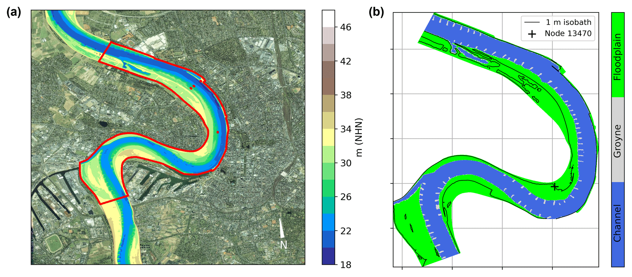
Figure 1Lower Rhine river topography and numerical model boundaries (red polygon) nearby Düsseldorf (a), and friction zones definition in the numerical model (b). The flow direction is north. (Satellite image a is the intellectual property of Esri and is used herein under license. Copyright © 2019 Esri and its licensors.)
4.1 Hydrodynamic model
A numerical model is used to simulate the flood scenario. In the BAW, studies carried out in large-scale river projects (101–102 km) usually make use of the hydrodynamic model TELEMAC-2D (Galland et al., 1991; Hervouet and Ata, 2017). It is a two-dimensional finite-element software (finite-volume also available) for solving the shallow water equations, a set of partial differential equations derived from the integration of the Navier–Stokes equations over the vertical axis. Thus, the equations for the conservation of mass and momentum in two dimensions should be solved.
where x and y are the Cartesian coordinates, h is the water depth, zb is the bottom elevation, u and v are the components of the velocity field, ν is the fluid viscosity (which may be constant or given by a turbulence model), τx,τy are the shear stress components, and Sx and Sy are any additional source term components of momentum (e.g. wind stress, external forces). The bottom shear stress is bound to the depth-averaged velocity by the quadratic law first introduced by Taylor and Shaw (1920):
The friction coefficient (cf) is equal to the sum of the bottom friction (cfb) and the friction due to vegetation (cfv). The bottom friction can usually be determined by traditional friction laws relating open-channel flow velocity to resistance coefficients (e.g. Manning, Chézy, Darcy–Weisbach, Nikuradse). However, on floodplains the velocity profile strongly depends on the vegetation height and morphology. Thus, specific flow resistance formulae have been developed for determining the vegetation drag (see Sect. 2).
The model consists of an unstructured triangular mesh composed of 56 825 points and 112 360 elements. The resolution varies from about 2.5 m in the main channel to about 30 m on the floodplains and the model mesh covers an area of ca. 8 km2. A constant discharge upstream and a constant water level downstream are imposed at the open boundaries, as mentioned above. A time step of 1 s guarantees a Courant number below 1 and it is used to simulate 24 h, which takes about 9 min with the LIND formulation using 160 processors of the BAW's high-performance computing system. The other three formulations for floodplain friction are about three times faster (3.5 min) as there is no iteration step.
This numerical model was extensively investigated from the point of view of sediment transport and morphodynamics (Backhaus et al., 2014; Riesterer et al., 2014), from which the calibrated hydrodynamic model was taken as a starting point for the current study. Water level measurements for a discharge of 7870 m3 s−1 available along the river channel axis were used to calibrate the bottom friction in the numerical model, as a representation of a flood scenario. A root mean square error (RMSE) smaller than 1 cm was accepted for the water level calibration. The bottom friction in the model defined by Nikuradse's equivalent sand roughness (ks) in the channel is set to 0.1 m. Originally the floodplains are divided into three basic categories: forest, cultivated land and meadows/pastures. In the current study, however, all the floodplain areas are considered to be covered with the same type of vegetation for the sake of simplicity (Fig. 1).
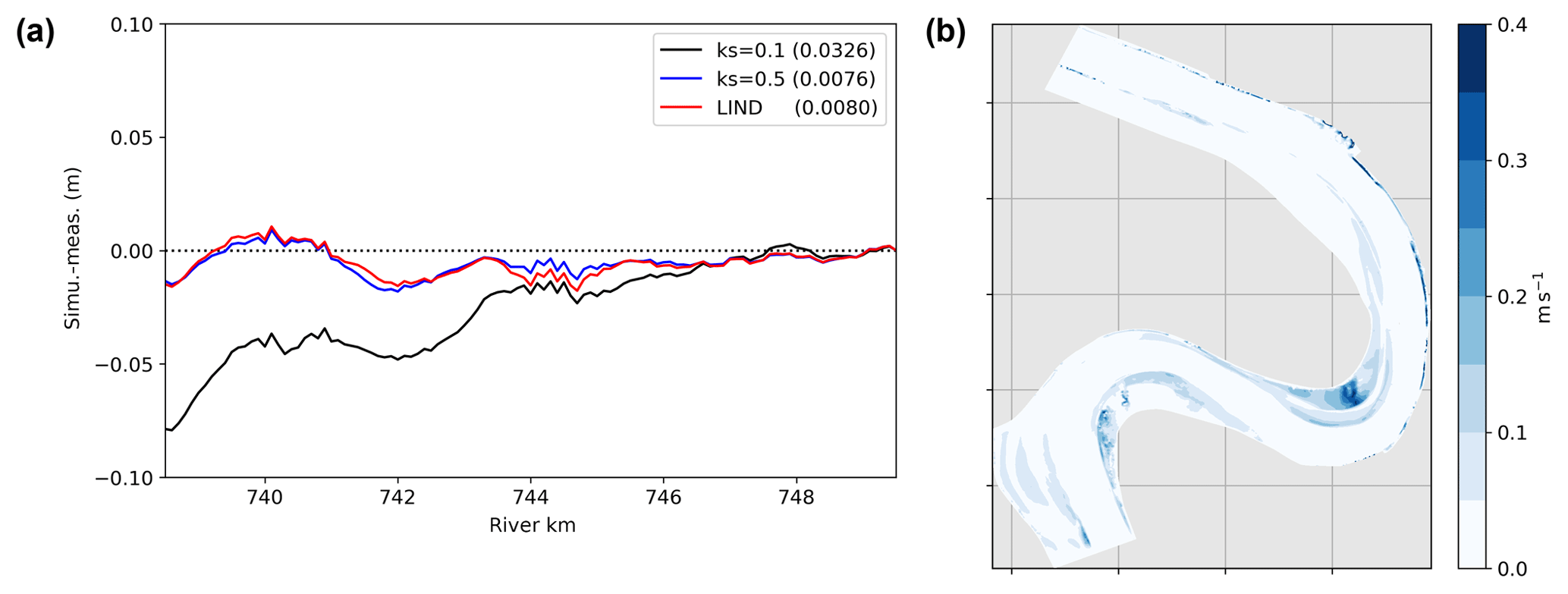
Figure 2Water level difference along the river channel axis for different floodplain friction values (a), and absolute difference of the flow velocity with and without floodplain friction formulation (b).
The calibration of the floodplain friction with water level measurements can be achieved either with (a) the traditionally used Lindner–Pasche friction law (Eq. 1) in addition to the bottom friction (Fig. 2a, red line) or (b) a higher bottom friction value on the floodplains (Fig. 2a, blue line). The calibration results are shown in Fig. 2. In (a) 5 cm thick stem evenly spaced by 5 m intervals are added to the floodplains with the LIND formulation, while keeping the bottom friction equal to the channel (red line). In (b) ks=0.5 m is used on the floodplains (blue line). In the case of the same friction value of the river channel (ks=0.1 m) being used for the floodplains, the momentum is too high and the simulated free surface does not fit the measurements (black line). In both cases the water level RMSE was reduced by a factor of 4 (see values within brackets).
The reader may ask himself or herself about which approach to be used. In this case it is useful to compare the absolute difference of the flow velocity with and without the floodplain friction formulation (see Fig. 2b). It can be seen that while differences in the main channel can be neglected (<0.05 m s−1), those on the floodplains cannot (up to 0.4 m s−1). In other words, when model calibration is based only on measurements in the river channel the hydrodynamics on floodplains is not guaranteed to be correctly simulated. It is important to point out that in the case of unsteady flow conditions a friction formulation dependent on water depth is not desired. However, if flow velocity measurements are not available on the floodplains (usually the case), little can be done in terms of calibration. Furthermore, remote sensing data of vegetation characteristics (light detection and ranging technology) have been used in flood modelling in the last 20 years, but the accuracy of these measurements should also be taken into account (see Cobby et al., 2003; Antonarakis et al., 2008; Dombroski, 2017).
An alternative to the deterministic approach in such situations, when there is a potential shortcoming in the modelling process due to a lack of information, is to carry out an UQ. As explained in Sect. 3, this analysis can be used to estimate the combined effect of all uncertain input parameters that significantly affect model results by means of a probabilistic approach.
4.2 Input parameters
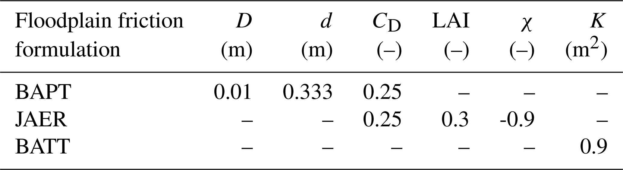
The next step now is to calibrate the remaining floodplain friction formulations with water level measurements. In order to make a comparison to the LIND approach, first H=10.0 m is set to ensure emergent conditions in all formulations. A second scenario is then calibrated for submerged conditions, in which H=1.0 m. Tables 1 and 2 present the calibrated parameters for each one of the scenarios. After the calibration all model results presented RMSE smaller than 1 cm for water level. (The density of stems m is calculated as 1∕d2, where d is the distance between stems.)
Table 1Floodplain friction parameter values calibrated under emergent conditions (H=10.0 m).
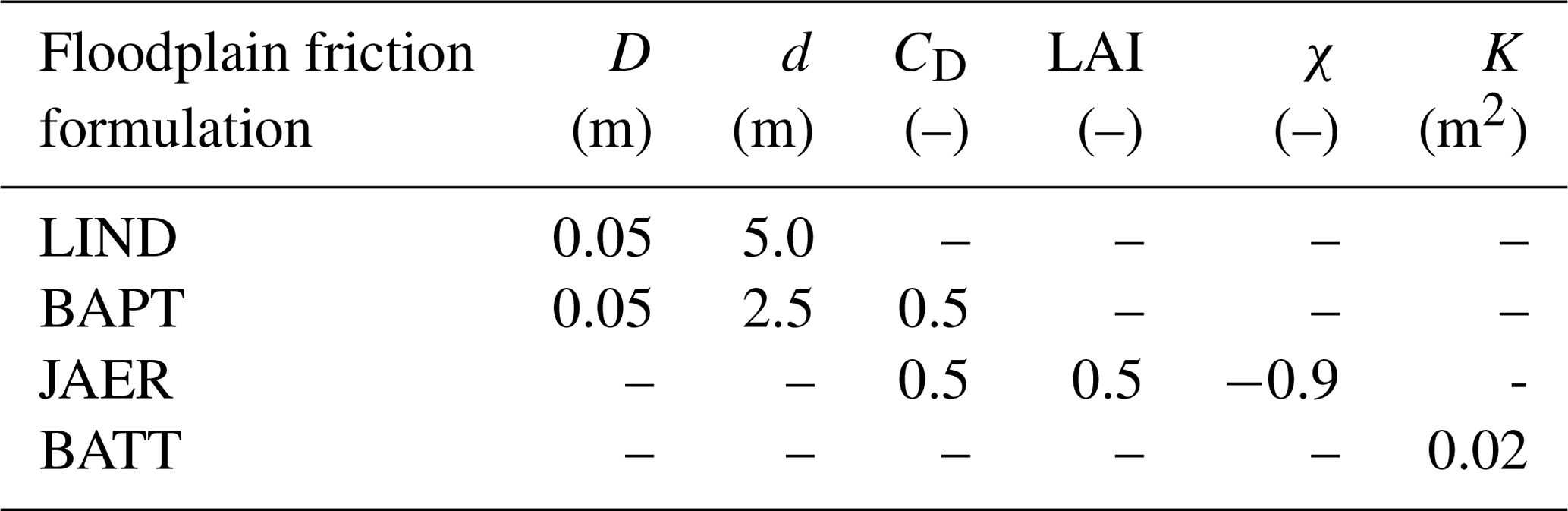
Table 2Floodplain friction parameter values calibrated under submerged conditions (H=1.0 m).
For the UQ it is required that all sensitive parameters relevant to model results should be considered for the determination of the PIs. Once the parameters are chosen a very important step follows: an error or deviation should be carefully assigned to each parameter. This variation should be small enough to be treated as an error, but large enough to include the actual parameter uncertainty (due to the lack of knowledge). Unfortunately there is no general rule for choosing a proper value, since different aspects might contribute, for example, measurement accuracy, spatial/time variances and numerical representation of process. In the current study, the chosen variations for the parameters related to the vegetation species (CD, LAI, χ) are based on values given in Aberle and Järvelä (2013) and Västilä and Järvelä (2014). For the remaining parameters (H, D, d, K) a standard deviation of 10 % of the calibrated value is assumed (σ=0.1μ). The vegetation height H is only included in the analysis under submerged conditions. Input deviations are treated as errors and, therefore, represented by a Gaussian distribution. This implies that there is a 99.7 % probability that the parameter value is found within .
Table 3Input parameter deviations and ranges.
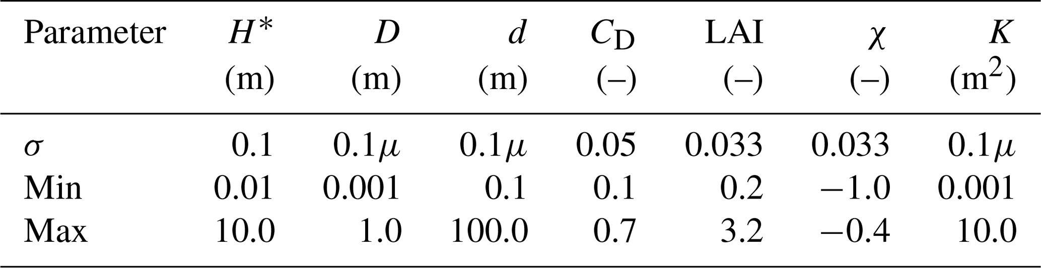
* Only for submerged conditions.
Finally, the UQ methods presented in Sect. 3 are applied with the input uncertainties given in Table 3. The FOSM method is evaluated through central finite difference; hence, 2n model evaluations are necessary (n refers to the number of input variables). For the MC method, a sample size of 1000 was used for the evaluation. Although MC sample sizes are usually considered in the range of 104–105, previous tests with 104 samples showed very little difference in results. The NIPC method (metamodelling) requires fewer samples than MC, because a polynomial function fitted to the samples is then used for the evaluation of results. In this case results with 100 samples for the metamodel were sufficient for approximating MC results.
The numerical model was evaluated with the four floodplain friction formulations. A constant discharge of 7870 m3 s−1 was imposed at the upstream boundary and at the downstream boundary a corresponding free surface based on a discharge curve. Model results were analysed after a steady state was achieved in the simulation and presented in the form of prediction interval (PI) with a 95 % probability of occurrence. It should be noted that the PI represents a range of variation around the mean value, which is not necessarily symmetric (MC and metamodelling). Once Monte Carlo results are available scatterplots can be used to investigate the behaviour of the model. They represent here the projection of the N values of model outputs against the N values of each of the n input parameters. Scatterplots are a very simple and informative form of sensitivity analysis, since they provide a visual representation of the relative importance of the input parameters (Saltelli et al., 2008). In order to summarize the scatterplots with a single value, standardized regression coefficients (SRCs) can be determined through linear regression.
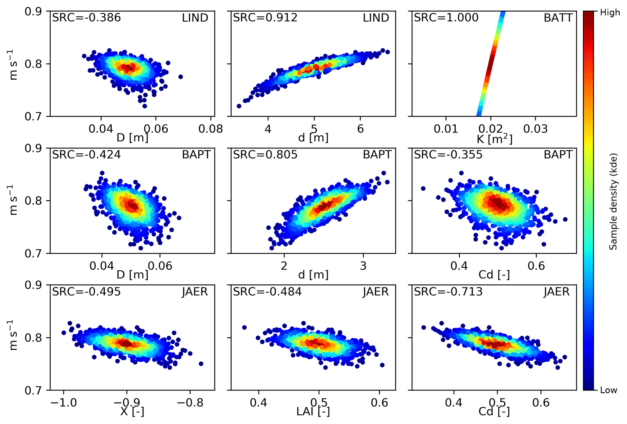
Figure 3Scatterplots of flow velocity results against floodplain friction input parameters at node 13470.
The scatterplots together with the SRCs are presented in Fig. 3, in which the sampled values of each input parameter (see Table 3) are plotted against the flow velocity results at node 13 470 (see Fig. 1) under emergent conditions. This node is considered representative of the hydrodynamics on vegetated floodplains. The SRC indicates whether there is a significant linear relation between input and output (values given in brackets). For instance the permeability coefficient (K) in BATT (1.0) is linearly related to the flow velocity, due to the approximation used under emergent conditions (see Sect. 2.4). The distance between stems (d) in LIND (0.912) and BAPT (0.805) also presents a significant linear effect on flow velocities. Interestingly the drag coefficient (CD) presents a much stronger linear relation to the flow velocity in JAER (−0.713) than in BAPT (−0.355). In summary the permeability coefficient (K), the distance between stems (d) and the drag coefficient (CD) in JAER were identified as inputs from the friction formulations with the largest linear effect on flow velocity. Although the remaining parameters showed no significant linear relation (), higher-order dependencies may still exist.

Figure 4Prediction interval of flow velocity under emergent conditions (rows: friction formulations; columns: UQ methods).
In Fig. 4 the UQ of the flow velocity under emergent vegetation conditions is presented. It can be observed that similar results are obtained with the three UQ methods. Among the friction formulations, LIND and JAER presented smaller variations on average and the PI exceeds 0.2 m s−1 only at the left floodplain in the middle of the river reach. On the other hand the BATT approach appears to be the most sensitive one, followed by BAPT. The approach from Battiato and Rubol (2014) results in PI >0.2 m s−1 on most of the floodplains. Relative to results with calibrated values all formulations showed variations above 10 % on the floodplains. The same analysis is carried out for submerged conditions (see Fig. 5). Because the LIND formulation is only valid for emergent conditions (independent of H), submerged conditions cannot be accounted for. As expected all results present on average larger PI than under emergent conditions, due to the addition of H in the analysis. The floodplain PI of flow velocity is mostly above 0.2 m s−1 and in BATT the PI >0.5 m s−1 is present on floodplains located at the inner bends of the river reach. In the channel the PI in BATT is the largest one and exceeds 0.05 m s−1 all along the upstream river section. Relative to results with calibrated values the variations now exceed 25 % on the floodplains, and in BATT at shallow regions up to 100 %.
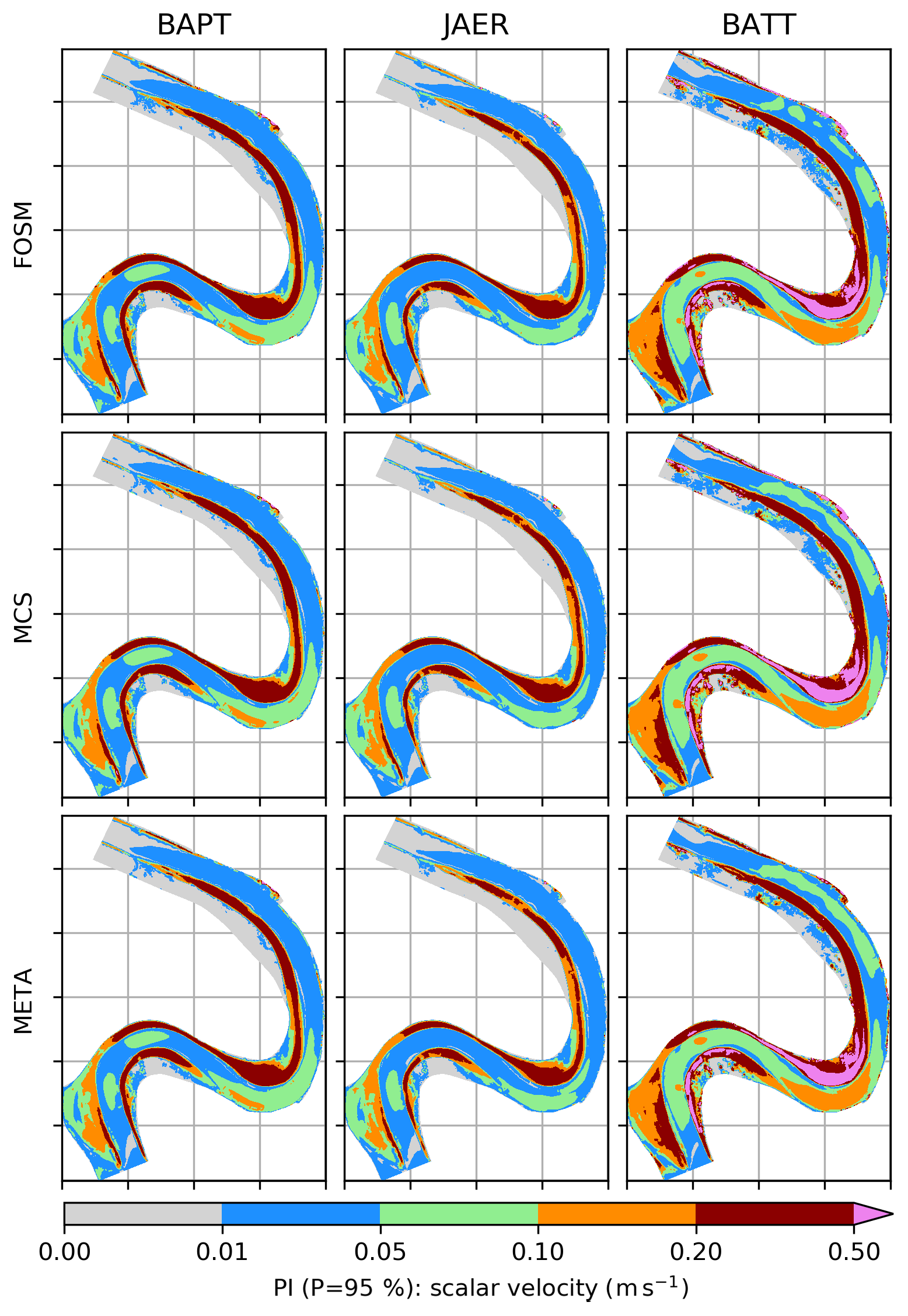
Figure 5Prediction interval of flow velocity under submerged conditions (rows: friction formulations; columns: UQ methods).
As explained in Sect. 3 results from the UQ can also be represented in terms of risk, i.e. a probability of failure (Pf). This is a more suitable analysis for when results must not exceed a given threshold. For instance, a threshold of 0.1 m s−1 above the mean value is used for the analysis of the flow velocity (see Fig. 6). In other words, the probability of exceedance of m s−1 was calculated. Because in the current study the difference among the UQ methods was not significant, results are now presented only from metamodelling. Results indicate that there is a larger probability that velocities are found above with the BATT approach. Under submerged conditions velocities are more likely to exceed this threshold. In BAPT and BATT the probability of failure can be higher than 10 % on the floodplains.
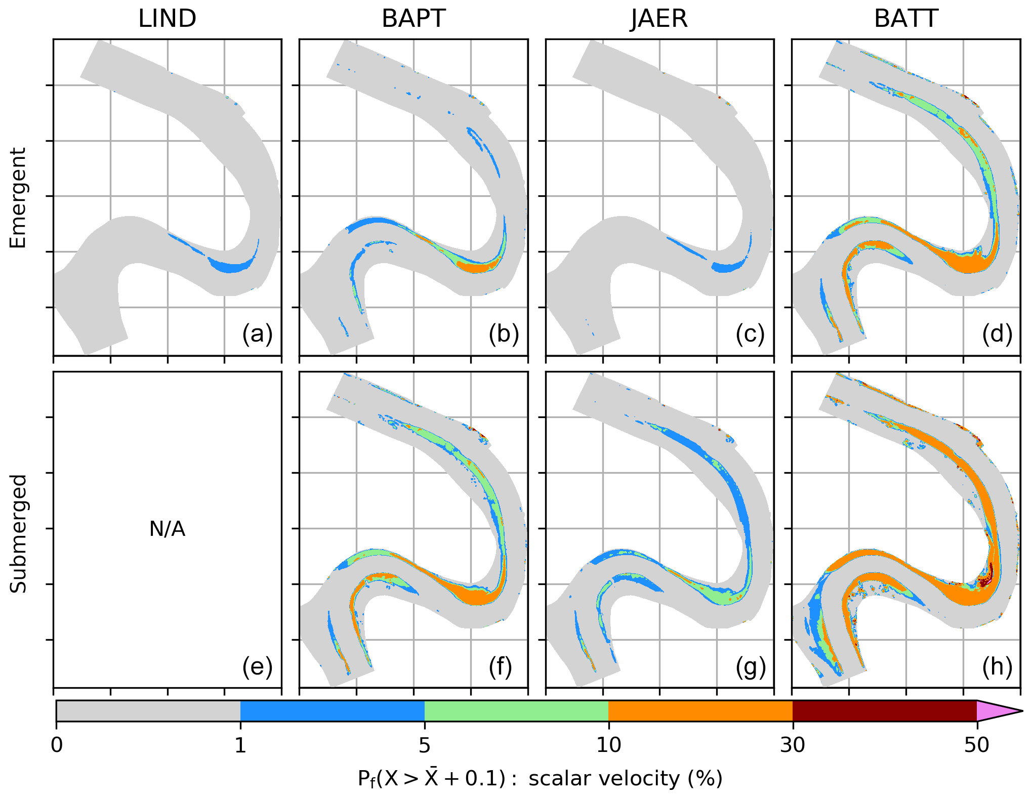
Figure 6Risk analysis of flow velocity for threshold m s−1 under emergent (a–d) and submerged (e–h) conditions.
Figures 4 and 5 show that results using the UQ methods are similar for this case study. Although the FOSM method is the least expensive alternative among the ones presented (only 2n model evaluations), it should be used with caution as it is a first-order method (linear approximation). In studies involving strongly dominant non-linear processes (e.g. turbulence modelling, sediment transport, unsteady conditions) further comparisons should be carried out. On the other hand, Monte Carlo-based methods have the advantage that the analysis under any conditions is possible. Although a large number of simulations is required for obtaining trustful results, alternatives such as the NIPC make them more feasible by reducing the sample size by at least 1 order of magnitude. For instance, Mouradi et al. (2016) carried out the UQ of a computationally intensive morphodynamic model, to which they applied pure MC and metamodelling methods.
When compared to emergent conditions the overall uncertainty of submerged conditions is significantly larger. This is an expected result in UQ as there is an additional input (vegetation height H) that significantly contributes to model performance. The Lindner–Pasche floodplain friction formulation is by definition only valid for emergent conditions. Thus, a different approach is needed when submerged conditions should be taken into account. Additionally, Brandimarte and Di Baldassare (2012) warn that when simulating flood scenarios attention must be given to parameter compensation between floodplain and channel resistance coefficients, so that reasonable values are chosen.
An important topic not only regarding UQ but numerical simulation in general, is the matter of input uncertainty definition. When performing a numerical simulation that is based on physical processes one will eventually need to validate calculations with measurements. Also, initial and boundary conditions are usually based on measurements of the original process. That is to say one should know a priori how accurate the available measurements are. This is usually not a trivial task, since measurement errors may not be easily evaluated (see Taylor, 1997). For instance, Di Baldassarre and Montanari (2009) published a study that focused only on the uncertainty in river discharge observations. Although it was attributed a standard deviation of 2.7 % for discharge measurement errors, the authors emphasize that this value is associated with their case study, and thus any generalization should be attributed with care. For uncertainties related to floodplain friction there are no such reference studies known to the authors. In that case, a suggested practice is to start with commonly used value ranges in the literature and apply a 6σ range () for the total parameter variation as a rule of thumb. Of course available experience in the topic of investigation should be also taken into account.
A framework for the estimation of uncertainties of hydrodynamic models on floodplains was presented. A traditional resistance formula used for river modelling together with three more recent approaches to floodplain friction were considered for carrying out an uncertainty quantification. The analysis was performed by means of three different methods: traditional MC, FOSM and NIPC (metamodelling). A two-dimensional model of a 10 km reach of the River Rhine was calibrated under steady flow conditions and the analysis was based on flow velocity results.
From the scatterplots it was identified that the permeability coefficient (K), the distance between stems (d) and the drag coefficient (CD) in JAER produce the largest linear effect on flow velocity among the inputs from the friction formulations. Altogether the tested floodplain friction formulae produced qualitatively similar results, in which uncertainties in flow velocity are most significant where the resistance coefficient was modified. Under emergent conditions, larger velocity variations are obtained with the formulations of BAPT and BATT. Variations from the latter also included the river channel. Under submerged conditions all approaches resulted in larger uncertainties, as the vegetation height was included in the analysis. Although the BATT approach presented once again the largest variations among the analysed methods, results were consistent not only qualitatively, but also quantitatively. In summary, among the tested floodplain friction formulae the JAER approach presented on average the smallest prediction intervals, i.e. the smallest variance. It is important to keep in mind that UQ results are not only dependent on the defined input parameter deviations, but also on the number of parameters considered in the analysis. In that sense, the BATT approach is still attractive as it reduces the current analysis to a single parameter, the canopy permeability K.
The three UQ methods compared gave similar results, which means that FOSM is the most efficient in this case. Despite being a very simple method to apply, FOSM will only produce good results when the first-order approximation is sufficient to describe the sensitivity of the system. In the presented study this was the case, probably because all the chosen inputs are directly correlated to the resistance coefficient. Research on related topics such as floodplain mapping usually focuses on the analysis of uncertainties that relies on Monte Carlo-based methods (e.g. Di Baldassarre et al., 2010; Domeneghetti et al., 2013). Several further topics could be listed here for future development, e.g. unsteady flow, boundary conditions, not to mention sediment transport modelling. However, the most important is first to be aware of the limitations of the available information and tools. Are there enough measurements for an acceptable calibration in the study area? Is the chosen numerical model capable of correctly representing the physical process under the desired conditions? As basic as it may sound, if those questions cannot be answered, any kind of analysis involving uncertainties will fail in providing useful results.
Model simulation and calibration data are available upon request from the corresponding author. Digital elevation model data are provided by the German Federal Waterways and Shipping Administration and are available under the terms of use for the provision of German federal geodata at https://atlas.wsv.bund.de/inspire/atom/hoehen.xml (German Federal Centre for Information Technology, 2017).
GLD designed the methodology and carried out the investigation with cooperation from all co-authors. TBZ provided the original model input data. RK contributed to the application of uncertainty quantification methods. GLD prepared the first draft of the manuscript, which was then revised and improved by the co-authors.
The authors declare that no competing interests are present.
The authors would like to thank the EDF researcher Cédric Goeury for his help with the metamodel set-up, and Audrey Valentine for her valuable comments in revising this paper. Moreover, we thank Renata Romanowicz and an anonymous referee for their coherent and constructive reviews.
This paper was edited by Giuliano Di Baldassarre and reviewed by Renata Romanowicz and one anonymous referee.
Aberle, J. and Järvelä, J.: Flow resistance of emergent rigid and flexible floodplain vegetation, J. Hydraul. Res., 51, 33–45, 2013. a, b
Aberle, J. and Järvelä, J.: Hydrodynamics of Vegetated Channels, Springer International Publishing, 519–541, 2015. a
Altarejos-García, L., Martínez-Chenoll, M. L., Escuder-Bueno, I., and Serrano-Lombillo, A.: Assessing the impact of uncertainty on flood risk estimates with reliability analysis using 1-D and 2-D hydraulic models, Hydrol. Earth Syst. Sci., 16, 1895–1914, https://doi.org/10.5194/hess-16-1895-2012, 2012. a
Antonarakis, A. S., Richards, K. S., Brasington, J., Bithell, M., and Muller, E.: Retrieval of vegetative fluid resistance terms for rigid stems using airborne lidar, J. Geophys. Res., 113, G02S07, https://doi.org/10.1029/2007JG000543, 2008. a
Apel, H., Thieken, A. H., Merz, B., and Blöschl, G.: Flood risk assessment and associated uncertainty, Nat. Hazards Earth Syst. Sci., 4, 295–308, https://doi.org/10.5194/nhess-4-295-2004, 2004. a
Backhaus, L., Brudy-Zippelius, T., Wenka, T., and Riesterer, J.: Comparison of morphological predictions in the Lower Rhine River by means of a 2-D and 3-D model and in situ measurements, in: Proceedings of the International Conference on Fluvial Hydraulics, RIVER FLOW, 2014, 1323–1330, 2014. a
Baptist, M. J., Babovic, V., Uthurburu, J. R., Keizer, M., Uittenbogaard, R. E., Mynett, A., and Verwey, A.: On inducing equations for vegetation resistance, J. Hydraul. Res., 45, 435–450, 2007. a, b, c, d
Battiato, I. and Rubol, S.: Single-parameter model of vegetated aquatic flows, Water Resour. Res., 50, 6358–6369, 2014. a, b, c, d, e, f
Baudin, M., Dutfoy, A., Iooss, B., and Popelin, A.-L.: OpenTURNS: An Industrial Software for Uncertainty Quantification in Simulation, in: Handbook of Uncertainty Quantification, edited by: Ghanem R., Higdon D., Owhadi H., Springer, Cham, 2017. a
Brandimarte, L. and Di Baldassare, G.: Uncertainty in design flood profiles derived by hydraulic modelling, Hydrol. Res., 43, 753–761, 2012. a, b
Cobby, D. M., Mason, D. C., Horritt, M. S., and Bates, P. D.: Two‐dimensional hydraulic flood modelling using a finite‐element mesh decomposed according to vegetation and topographic features derived from airborne scanning laser altimetry, Hydrol. Process., 17, 1979–2000, 2003. a
Dettinger, M. D. and Wilson, J. L.: First order analysis of uncertainty in numerical models of groundwater flow part: 1. Mathematical development, Water Resour. Res., 17, 149–161, 1981. a
Di Baldassarre, G. and Montanari, A.: Uncertainty in river discharge observations: a quantitative analysis, Hydrol. Earth Syst. Sci., 13, 913–921, https://doi.org/10.5194/hess-13-913-2009, 2009. a
Di Baldassarre, G., Schumann, G., Bates, P. D., Freer, J. E., and Beven, K. J.: Flood-plain mapping: a critical discussion of deterministic and probabilistic approaches, Hydrolog. Sci. J., 55, 364–376, 2010. a, b
Dombroski, D.: Remote Sensing of Vegetation Characteristics for Estimation of Roughness in Hydraulic Modeling Applications, Tech. Rep. ST-2017-6034-01, U.S. Department of the Interior, Bureau of Reclamation, Denver, 2017. a
Domeneghetti, A., Vorogushyn, S., Castellarin, A., Merz, B., and Brath, A.: Probabilistic flood hazard mapping: effects of uncertain boundary conditions, Hydrol. Earth Syst. Sci., 17, 3127–3140, https://doi.org/10.5194/hess-17-3127-2013, 2013. a, b
DVWK: Hydraulische Berechnung von Fließgewässern, no. 220 in DVWK-Merkblätter zur Wasserwirtschaft, Deutsche Verband für Wasserwirtschaft und Kulturbau e.V., Bonn, 1991. a
Galland, J.-C., Goutal, N., and Hervouet, J.-M.: TELEMAC: A new numerical model for solving shallow water equations, Adv. Water Resour., 14, 138–148, 1991. a
German Federal Centre for Information Technology: Niederrhein und Unter-/Aussenems: Digitales Höhenmodell des Wasserlaufs (DGM-W), available at: https://atlas.wsv.bund.de/inspire/atom/hoehen.xml, last access: 14 June 2017. a, b
Hervouet, J.-M. and Ata, R.: User manual of opensource software TELEMAC-2D, available at: http://www.opentelemac.org (last access: 2 July 2018), v7P2, 2017. a
Hosder, S. and Walters, R.: Non-Intrusive Polynomial Chaos Methods for Uncertainty Quantification in Fluid Dynamics, in: Proc. 48th AIAA Aerospace Sciences Meeting Including the New Horizons Forum and Aerospace Exposition, 2010. a
Järvelä, J.: Determination of flow resistance caused by non-submerged woody vegetation, Intl. J. River Basin Management, 2, 61–70, 2004. a, b, c, d, e
Lindner, K.: Der Strömungswiderstand von Pflanzenbeständen, Technische Universität Braunschweig. Leichtweiss-Institut für Wasserbau: Mitteilungen, Leichtweiss-Inst. f. Wasserbau d. Techn. Univ. Braunschweig, Braunschweig, 1982. a, b, c
LUA: Hochwasserabflüsse bestimmter Jährlichkeit HQT an den Pegeln des Rheins, Tech. Rep. 1610-9619, Landesumweltamt Nordrhein-Westfalen, Essen, 2002. a
Marelli, S. and Sudret, B.: UQLab user manual – Polynomial Chaos Expansions, Tech. Rep. UQLab-V1.0-104, Chair of Risk, Safety & Uncertainty Quantification, ETH, Zurich, 2017. a
Mouradi, R.-S., Audouin, Y., Goeury, C., Claude, N., Tassi, P., and Abderrezzak, K. E. K.: Sensitivity analysis and uncertainty quantification in 2D morphodynamic models using a newly implemented API for TELEMAC2D/SISYPHE, in: 23rd Telemac-Mascaret User Club, 2016. a
Nikora, N., Nikora, V., and O'Donoghue, T.: Velocity Profiles in Vegetated Open-Channel Flows: Combined Effects of Multiple Mechanisms, J. Hydraul. Eng., 45, 435–450, 2007. a
Pappenberger, F., Beven, K., Horritt, M., and Blazkova, S.: Uncertainty in the calibration of effective roughness parameters in HEC-RAS using inundation and downstream level observations, J. Hydrol., 302, 46–69, 2005. a
Pasche, E.: Turbulenzmechanismen in naturnahen Fließgewässern und die Möglichkeiten ihrer mathematischen Erfassung, Lehrstuhl f. Wasserbau u. Wasserwirtschaft u. Inst. f. Wasserbau: Mitteilungen, Inst. für Wasserbau u. Wasserwirtschaft, Rhein.-Westfäl. Techn. Hochsch., Aachen, 1984. a, b, c
Riesterer, J., Wenka, T., Oberle, P., and Brudy-Zippelius, T.: Numerische Modellierung des Geschiebetransports in gekrümmten Gerinnen, in: Simulationsverfahren und Modelle für Wasserbau und Wasserwirtschaft: 37. Dresdner Wasserbaukolloquium 2014, 13–14 März 2014, Hrsg.: Mietz, S.-C., vol. 50 of Dresdner wasserbauliche Mitteilungen, 121–130, TU, Dresden, 2014. a
Rouse, H.: Critical Analysis of Open-Channel Resistance, Journal of the Hydraulics Division, 91, 1–23, 1965. a
Rubol, S., Ling, B., and Battiato, I.: Universal scaling-law for flow resistance over canopies with complex morphology, Sci. Rep.-UK, 8, 4430, https://doi.org/10.1038/s41598-018-22346-1, 2018. a
Saltelli, A., Ratto, M., Andres, T., Campolongo, F., Cariboni, J., Gatelli, D., Saisana, M., and Tarantola, S.: Global sensitivity analysis: the primer, John Wiley, Chichester, UK, 2008. a
Shields, F. D., Coulton, K. G., and Nepf, H.: Representation of Vegetation in Two-Dimensional Hydrodynamic Models, J. Hydraul. Eng., 143, 02517002, https://doi.org/10.1061/(ASCE)HY.1943-7900.0001320, 2017. a, b, c
Sitar, N., Cawlfield, J. D., and Der Kiureghian, A.: First-order reliability approach to stochastic analysis of subsurface flow and contaminant transport, Water Resour. Res., 23, 794–804, 1987. a
Straatsma, M. and Huthoff, F.: Relation between accuracy of floodplain roughness parameterization and uncertainty in 2D hydrodynamic models, Tech. rep., Foundation Flood Control 2015, 2010. a
Taylor, G. I. and Shaw, W. N.: I. Tidal friction in the Irish Sea, Philos. T. R. Soc. Lond., 220, 1–33, 1920. a
Taylor, J.: An Introduction to Error Analysis: The Study of Uncertainties in Physical Measurements, ASMSU/Spartans.4.Spartans Textbook, University Science Books, 1997. a
Västilä, K. and Järvelä, J.: Modeling the flow resistance of woody vegetation using physically based properties of the foliage and stem, Water Resour. Res., 50, 229–245, 2014. a
Walters, R. and Huyse, L.: Uncertainty analysis for fluid mechanics with applications, Tech. Rep. 2002-1, Institute for Computer Applications in Science and Engineering, Hampton: ICASE, NASA Langley Research Center, 2002. a, b
Willis, T. D. M., Wright, N. G., and Sleigh, P. A.: Uncertainty with friction parameters and impact on risk analysis, in: Proc. 3rd European Conference on Flood Risk Management, vol. 7, p. 04011, 2016. a
Yen, B. C.: Open Channel Flow Resistance, J. Hydraul. Eng., 128, 20–39, 2002. a
Yen, B. C., Cheng, S. T., and Melching, C. S.: First order reliability analysis, Stochastic and risk analysis in hydraulic engineering, Water Resources Publications Littleton, US, 1–36, 1986. a