the Creative Commons Attribution 4.0 License.
the Creative Commons Attribution 4.0 License.
 | 13 Aug 2019
Assessing the influence of soil freeze–thaw cycles on catchment water storage–flux–age interactions using a tracer-aided ecohydrological model
Doerthe Tetzlaff
Hjalmar Laudon
Marco Maneta
Chris Soulsby
Ecohydrological models are powerful tools to quantify the effects that independent fluxes may have on catchment storage dynamics. Here, we adapted the tracer-aided ecohydrological model, EcH2O-iso, for cold regions with the explicit conceptualization of dynamic soil freeze–thaw processes. We tested the model at the data-rich Krycklan site in northern Sweden with multi-criterion calibration using discharge, stream isotopes and soil moisture in three nested catchments. We utilized the model's incorporation of ecohydrological partitioning to evaluate the effect of soil frost on evaporation and transpiration water ages, and thereby the age of source waters. The simulation of stream discharge, isotopes, and soil moisture variability captured the seasonal dynamics at all three stream sites and both soil sites, with notable reductions in discharge and soil moisture during the winter months due to the development of the frost front. Stream isotope simulations reproduced the response to the isotopically depleted pulse of spring snowmelt. The soil frost dynamics adequately captured the spatial differences in the freezing front throughout the winter period, despite no direct calibration of soil frost to measured soil temperature. The simulated soil frost indicated a maximum freeze depth of 0.25 m below forest vegetation. Water ages of evaporation and transpiration reflect the influence of snowmelt inputs, with a high proclivity of old water (pre-winter storage) at the beginning of the growing season and a mix of snowmelt and precipitation (young water) toward the end of the summer. Soil frost had an early season influence of the transpiration water ages, with water pre-dating the snowpack mainly sustaining vegetation at the start of the growing season. Given the long-term expected change in the energy balance of northern climates, the approach presented provides a framework for quantifying the interactions of ecohydrological fluxes and waters stored in the soil and understanding how these may be impacted in future.
- Article
(2125 KB) - Full-text XML
-
Supplement
(1797 KB) - BibTeX
- EndNote


Northern watersheds are sensitive hydrologic sites where a significant proportion of the annual water balance is controlled by the spring melt period (Kundzewicz et al., 2007) and can thus be key sentinels for detecting climate change impacts (Woo, 2013). Recent data and long-term climate projections indicate a significant increase in warming for extensive areas of boreal forests currently experiencing low-energy, low-precipitation hydroclimatic regimes (Pearson et al., 2013). The limited number of long-term monitoring sites with high-quality data is a concern because it may prove difficult to document the anticipated hydrological change in these catchments (Laudon et al., 2018; Tetzlaff et al., 2015). Within changing northern catchments, with high water loss due to transpiration ( %) (Schlesinger and Jasechko, 2014), and significant influence of evapotranspiration (ET) fluxes on streamflow (Karlsen et al., 2016a), the long-term ecohydrological implications of vegetation adaptation, plant water use, and the water sources that sustain growth are crucial to understand and quantify. Vegetation in boreal regions also exerts strong influences on the energy balance of such catchments, with low leaf area index (LAI) conifer forests and shrubs affecting the surface albedo, snow interception and the timing and duration of the largest input fluxes of water during snowmelt (Gray and Male, 1981). However, the interactions between soil water storage and “green water” fluxes of transpiration and evaporation are poorly constrained in northern regions, and the way in which sources of water from inputs of snowmelt and summer rainfall mix and sustain plant growth is only just beginning to be understood (Sprenger et al., 2018a). Assessment of these interactions in northern catchments is further complicated by large temperature variations, and the resulting stagnation of hydrological processes induced by frequent frozen ground conditions. With increasing temperatures and potential changes to the winter soil freeze–thaw dynamics (e.g. Venäläinen et al., 2001), it is important to establish how these affect current vegetation–soil water interactions to project the implications of future change.
The intricate complexities of changes in the land surface energy balance, temporal changes in sub-surface storage due to frost conditions, and vegetation and soil water usage (transpiration and soil evaporation, respectively) are notoriously challenging to continuously monitor (Maxwell et al., 2019), particularly in northern environments, where site access is typically remote and extreme cold can limit in situ monitoring devices. In these circumstances, the fusion of sparsely available data with hydrological models is an effective method to quantify water fluxes and storage dynamics at different temporal and spatial scales. While the calibration of such models requires significant hydrometric data inputs, recent work has shown that incorporation of stable isotopes can be an effective tool for constraining the model estimations of storage–flux interactions in the absence of direct in situ measurements. Such models include (but are not limited to) the STARR (Spatially distributed Tracer-Aided Rainfall-Runoff) model (van Huijgevoort et al., 2016), which was developed for tracer-aided simulations and calibration and adapted for additional cold-region processes (Ala-Aho et al., 2017, 2018; Piovano et al., 2018), CRHM (Cold Regions Hydrologic Model) specific to cold regions (Pomeroy et al., 2007), but not currently using tracers, the isoWATFLOOD model (Stadnyk et al., 2013), which has been used to isolate water fluxes with tracer-aided modelling in large-scale applications in northern regions of Canada, and the EcH2O-iso model (Maneta and Silverman, 2013; Kuppel et al., 2018a, b), which was developed as a process-based, coupled atmosphere–vegetation–soil energy-balance ecohydrologic model and modified to incorporate isotopic tracers (stable isotopes deuterium and oxygen-18, δ2H and δ18O, respectively). However, apart from EcH2O-iso, which explicitly conceptualizes short-term (diurnal and seasonal) and long-term (growth-related) vegetation dynamics and biomass productivity, most of these existing models were mainly developed with a focus on runoff generation (“blue water” fluxes). Consequently, they have a very simplistic representation of vegetation–soil–water interactions, estimating ET by approximating the physical transpiration controls of vegetation (e.g. Penman–Monteith and Priestley–Taylor methods) and partitioning fluxes after estimation of actual ET (Fatichi et al., 2016).
Currently, EcH2O-iso already incorporates some cold-region processes, namely snowpack development, a snowmelt routine, and the influence of temperature effects on vegetation productivity. While the depth of the snowpack is not directly estimated (only snow water equivalent is tracked), the surface energy balance incorporates snowpack heat storage to estimate the warming phase with effective snowmelt timing (Maneta and Silverman, 2013). The model additionally estimates soil temperature; however, freezing temperature and soil frost development are adaptations that are needed for use in catchments with extensive freezing conditions. Soil freeze–thaw has the potential to significantly influence soil moisture conditions, tracer dynamics, and the magnitude and ages of all water fluxes. Soil freeze–thaw cycles have been estimated with a variety of methods, ranging from the Stefan equation (i.e. cumulative freezing temperatures) to the more physically based Richards–Fourier calculations (e.g. Zhang et al., 2007; Zhang and Sun, 2011). The simplicity of the Stefan equation is useful in many circumstances, including where computational efficiency is important (as with EcH2O-iso), which restricts the use of small time and space steps of physically based models. Additionally, the Stefan equation works well in most environments when soil latent heat is much larger than the sensible heat and there are linear gradients of soil temperature (Jumikis, 1977). The incorporation of tracer dynamics into EcH2O-iso opens opportunities to strengthen the evaluation of the model processes (Kuppel et al., 2018b) and permits the use of tracers in calibration (Douinot et al., 2019). Here, our overall aim was to provide a framework for assessing vegetation influences on the hydrology of cold regions by adapting the EcH2O-iso model and testing it in the intensively monitored Krycklan catchment in northern Sweden. The specific objectives of the study are 3-fold: (1) to assess the capability of a spatially distributed, physically based ecohydrological model to capture the influence of snow and soil freeze–thaw processes on water storage dynamics, and the resulting flux magnitudes under different vegetation communities (forest vs. mire), (2) to examine the influence of soil frost on the dynamics and age of water fluxes within the catchment, and (3) to provide a generic modelling approach for application to other frost-affected catchments. In the adaptation of EcH2O-iso to cold regions and the assessment of the simulated vegetation–soil water interactions with frost conditions, we aim to improve the understanding and projection of the future role of vegetation in cold-region hydrology.
2.1 EcH2O-iso model
Recent advances in hydrological modelling have included more explicit process-based conceptualization of ecohydrological interactions (Fatichi et al., 2016) and the integration of tracer-based data (Birkel and Soulsby, 2015). The EcH2O model (Maneta and Silverman, 2013) was developed as an ecohydrological model coupling land-surface energy-balance models with a physically based hydrologic model. This explicitly includes the dynamics of vegetation growth and vertical and lateral ecohydrological exchanges.
2.1.1 EcH2O energy balance
The energy balance is computed for two layers, the canopy and the surface. The solution of the energy balance is used to calculate the available energy reapportionment for transpiration, interception evaporation, soil evaporation, snowmelt, ground heat storage, and canopy and soil temperature. The canopy energy balance is iteratively solved at each time step until canopy temperature converges to the estimated value that balances radiative (incoming and outgoing short- and long-wave radiation) and turbulent energy fluxes (sensible and latent heat) (Maneta and Silverman, 2013; Kuppel et al., 2018a, b). Long- and short-wave radiation transmitted through the canopy to the soil and long-wave radiation emitted by the canopy toward the ground drive the surface energy balance. The surface energy-balance components include radiative exchanges (incoming and outgoing short- and long-wave radiation), sensible, latent, and ground heat fluxes, as well as heat storage in the soil and in the snowpack. Soil evaporation is estimated with the latent heat, using the atmospheric conditions (air density and heat capacity), soil resistance to evaporation, and the aerodynamic resistance (surface and canopy) of the evaporative surface (Maneta and Silverman, 2013). The transpiration is estimated at the leaf and is dependent on the vapour pressure gradient from the leaf to the atmosphere, the canopy resistance to vapour transport, vegetation properties, and the current soil saturation conditions (Maneta and Silverman, 2013). While the energy balance apportions energy to each storage (i.e. soil and snowpack), when the snowpack is present, estimated surface temperatures refer to the snowpack surface, and the surface temperature of the ground is assumed to be at the temperature of the snowpack, which means that conductive heat transfer between soil and snowpack is 0 (no thermal gradient). Also, when the snowpack is present, latent heat for surface evaporation is set to 0. When no snowpack is present, the ground heat flux (and soil temperature) is estimated with the one-dimensional (1-D) diffusion equation with two thermal layers, where the bottom of the top thermal layer is estimated with the thermal conductivity and heat capacity of the thermal layer (Maneta and Silverman, 2013). The 1-D diffusion equation is only used during the snow-free conditions since soil frost causes discontinuities in the estimation of the thermal layers. While soil temperature is estimated within EcH2O (at the interface of the first and second soil thermal layers), there is currently no freezing routine for soil water below 0 ∘C.
2.1.2 EcH2O-iso tracer and water age module
EcH2O has previously been adapted to incorporate the tracking of hydrological tracers including stable isotopes (Kuppel et al., 2018b) and chloride (Douinot et al., 2019), and adapted to compute estimations of water age in water storage and fluxes. Isotopic fractionation is simulated in soil water using the Craig–Gordon model (Craig and Gordon, 1965), and tracer mixing is simulated using an implicit first-order finite-difference scheme. Full details of the implementation of the isotopic module are in Kuppel et al. (2018a). These adaptations do not consider fractionation of snowmelt or open water evaporation. Water ages are estimated assuming complete mixing in each water storage compartment. Similar to other snowmelt tracer models (e.g. Ala-aho et al., 2017), the snowmelt ages are defined as the time the snow enters the catchment, rather than the time of melt. This results in older water estimations during the freshet period and a more complete estimate of the time that water has resided in the catchment.
2.2 Soil water freeze–thaw adaptation
Hydrology in cold regions can be greatly affected by the freeze–thaw cycles of soil water during the winter, resulting in reduced liquid water storage capacity during the spring melt and a restricted capability for infiltration due to the expansion of ice in pore spaces (Jansson, 1998). The depth of the soil frost can have a large influence on the timing of snowmelt runoff and can provide an estimation of the liquid water available within a soil layer (Carey and Woo, 2005). The Stefan equation is a simple energy-balance approach to estimate the progression of soil water freezing (Jumikis, 1977):
where Δz)f (m) is the change in depth of the frost and is a function of the thermal conductivity of the frozen soil layers between the frost depth and the soil surface (kf, W m−1 ∘C−1), the soil surface temperature below the snowpack (Ts, ∘C), the temperature of freezing (Tf, ∘C), the latent heat of freezing (λ, J m−3), and the liquid soil moisture (θ, m3 m−3). As with previous approaches (Jumikis, 1977; Carey and Woo, 2005), the progression of the soil frost is estimated by discretizing the total soil depth into smaller layers. Within EcH2O-iso, the sub-surface soil regime is discretized into three soil layers, layer 1 (near the surface), layer 2, and layer 3 (groundwater to bedrock), to resolve the water balance and estimate soil moisture. Here, the depths of layers 1, 2, and 3 were used as the layers since they intrinsically incorporate the soil moisture estimations without additional parameterization. The thermal conductivity of frost-affected layers is dependent on the moisture content of the soil:
where kf(i) (W m−1 ∘C−1) is the thermal conductivity of frozen soil in layer i, ksat (W m−1 ∘C−1) is the thermal conductivity of saturated soil, kdry (W m−1 ∘C−1) is the thermal conductivity of dry soil, θ(i) (m3 m−3) is the soil moisture in layer i, and ϕ(i) (m3 m−3) is the soil porosity in layer i. The saturated thermal conductivity was estimated from the proportions of soil comprised of ice, liquid water, air, organic material, and mineral soil (Carey and Woo, 2005):
where j is the thermal conductivity of each volume proportion, f is the fraction of total soil volume, and k is the thermal conductivity of volume j. Without proportions of soil organic and mineral material, the bulk soil thermal conductivity (kdry) is considered the weighted average of organic and mineral thermal conductivity (only four total volumes in Eq. 3). Implementations of Eqs. (1)–(3) for freezing layers below the ground surface are ideal for EcH2O as the model estimates the parameters (Ts and θ) or includes parameterization of physical properties (λ, kdry, ϕ, kwater, kair), and only requires the addition of the thermal conductivity of ice (2.1 W m−1 ∘C−1, Waite et al., 2006). Within EcH2O, the estimation of surface temperature (above the snowpack) is assumed to be isothermal with the snowpack and conduction through the snowpack is not considered. However, conduction through snowpack is important for the Stefan equation (Eq. 1) as the surface temperature used is below the snowpack, which is generally thermally insulated by the snowpack. To address the conduction through the snowpack without snow depth or density, the estimated surface temperature above the snowpack (TEst) was damped with a single unitless parameter (D) such that . To account for the reduction of the infiltration rate due to ice, models have previously adjusted the soil hydraulic conductivity (e.g. Jansson, 1998). Here, the reduction in hydraulic conductivity is estimated using an exponential function:
where Kwf (m s−1) is the hydraulic conductivity of the soil influenced by ice, Ksat (m s−1) is the saturated hydraulic conductivity of ice-free soils, fc is a unitless ice-impedance parameter, and F is the fraction of frost depth to total soil depth. Equation (4) has two key assumptions: no ice lenses or frost heaving, and no soil volume expansion due to lower ice density (assumed 920 kg m−3 at ice temperature 0–5 ∘C).
2.3 Soil frost volume, depth, and water age
As soil frost progresses through the layers, the proportion of liquid water is assumed to decrease at the same rate as the proportion of unfrozen soil. Similar to other approaches estimating the moisture content of frost-affected soils (Jansson, 1998), a minimum liquid soil moisture was retained in all frozen soils. This minimum was assumed to be the residual soil moisture (θr), the minimum moisture content required for evaporation and root uptake. Following the estimation of the soil water infiltration and redistribution of soil water within EcH2O, the change in soil moisture due to freezing in each layer is estimated:
where Δθ (m3 m−3) is the change in liquid water and ice content, θ(i) (m3 m−3) is the initial liquid content in layer i, θr (m3 m−3) is the residual moisture content, d(i) (m) is the total depth of layer i, and dF(i) (m) is the depth of frost in layer i. Step-wise estimation of freeze and thaw for each layer is provided in more detail in Sect. S1 in the Supplement. The water age of the ice is estimated in a similar way to the liquid water ages of the soil layers (Kuppel et al., 2018b):
where t is time (s), Δt is the time step (s), Vres (m3) is the volume of ice in storage, qin (m3) is the volume of water from the change in soil moisture during freeze-up (using Δθ in Eq. 5), qout (m3) is the volume of water from the change in soil moisture during thaw (from Eq. 5), and A (s) is the water age (subscripts “res” and “in” are the water ages in storage and inflow, respectively). Similar to the isotope and vegetation modules in EcH2O, the frost dynamics (i.e. frost depths and water ages) were implemented as an option within EcH2O.
2.4 Isotope snowmelt fractionation
Isotopic fractionation of snowmelt can have a significant influence on the composition of streams (Ala-aho et al., 2017). Previous successful applications of a simple approach equation to estimate the isotopic fractionation of snowmelt at multiple locations have shown that low-parameterized fractionation models can be used to spatially approximate snowmelt fractionation. One of the noted limitations of the simple snowmelt fractionation approach used in Ala-aho et al. (2017) is the dependence of the snowmelt fractionation on the past snowmelt volumes (total days of melt, dmelt) rather than current snowmelt rate (); Mfrac is a fractionation parameter in Ala-aho et al. (2017). The approach was modified to include the snowmelt rate with one additional parameter using an exponential function:
where δ2Hmelt (‰) is the isotopic composition of the snowmelt, δ2Hpack (‰) is the composition of the snowpack at the beginning of the time step, SWE (m) is the snow water equivalent at the current time, SWEmax (m) is the maximum snow water equivalent before melt, M (m) is the total depth of snowmelt in the current time step, S is a unitless slope parameter describing the shape of the exponential change in the snowmelt fractionation, and C (‰) is an amplification factor. Equation (7) serves as the mass balance for the snowpack isotopes throughout the winter and spring melt period. In comparison to Ala-aho et al. (2017), the exponential form works to temporally change the shape of the fractionation as a relationship with the amount of melt (i.e. replacing 1∕dmelt). Higher values of S (10–20) result in larger early melt fractionation and limited late melt fractionation, while low values of S result in a lower but more consistent fractionation throughout the melt period. The amplification factor behaves as a simplification of atmospheric effects on the snowmelt fractionation. The isotopic composition of the snowpack is updated at the end of each time step.
3.1 Study site
Svartberget (C7, 0.49 km2) is a small subcatchment situated in the headwaters of the Krycklan catchment (64∘14′ N, 19∘46′ E) in northern Sweden. Svartberget is a well-studied site with long-term data collection including streamflow (1991–present), stream chemistry (2000–present), and hillslope transect measurements (soil moisture and water chemistry). Svartberget has two subcatchments, Västrabäcken (C2, 0.12 km2) and mire (C4, 0.18 km2) (Fig. 1). The topographic relief of C7 is 71 m (235–306 m a.s.l.), with 57 m of relief in C2 (247–304 m a.s.l.) and only 26 m of relief in C4 (280–306 m a.s.l.) (Fig. 1). The climate is subarctic (in the Köppen classification index), with annual precipitation of 614 mm, evapotranspiration (ET) of 303 mm, mean relative humidity of 82 %, and a 30-year mean annual temperature of 1.8 ∘C (Laudon et al., 2013). The relatively low topography results in no observable influence of elevation on precipitation (Karlsen et al., 2016b). The catchment experiences continuous snowpack development throughout the winter, accounting for approximately a third of the annual precipitation and lasting on average 167 d (Laudon and Ottosson Löfvenius, 2016). The large quantity of snowfall results in a dominant snowmelt-driven freshet period (Karlsen et al., 2016a). Till (10–15 m thick) covers the majority of the downstream catchment area (C7, 92 % downstream of C4) with intermittent shallow soils in the headwaters of C2 (Fig. 1a). The catchment is predominantly forest-covered (82 % total, 98 % downstream of C4), with Scots pine (Pinus sylvestris), Norway spruce (Picea abies), and birch (Betula spp.). The mire (Fig. 1b) is dominated by Sphagnum mosses.
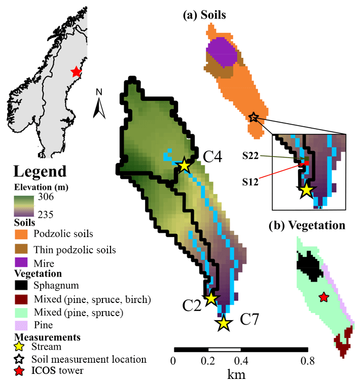
Figure 1Location of the Svartberget within Sweden and its elevation profile with the channels and stream measurement locations (yellow). Inset figures show (a) catchment soils with the locations of S12 and S22, and (b) catchment vegetation.
3.2 Input and calibration datasets
3.2.1 Stream discharge and isotope datasets
The discharge at the three streamflow locations has been measured with hourly stream stage measurements using pressure transducers. V-notch weirs improve measurement accuracy, aided by monthly salt dilution gauging to validate results. Average discharge in the catchment varies from m3 s−1 (C2) to m3 s−1 at the outlet (C7), with maximum discharge events up to 0.1 m3 s−1 (C7) during spring freshets (0.02 and 0.03 m3 s−1 at C2 and C4, respectively). The evaluation of the stable isotopes δ2H and δ18O of stream water was carried out for the stream water samples collected every 2 weeks at each site. Long-term average δ2H is similar between streams (−95.5 ‰, −94.5 ‰, and −95.6 ‰ for C7, C2, and C4, respectively), with the highest isotopic variability at site C4 – standard deviation (SD) of 7.9 ‰ – and lowest at C2 (SD of 4.5 ‰) with C7 intermediate.
3.2.2 Meteorological datasets
Precipitation (rain and snowfall), temperature, wind speed, and relative humidity were measured daily at the Svartberg meteorological station, 150 m south-west of the catchment. Radiation data, incoming long-wave and short-wave radiation, were obtained at 3-hourly time steps and 0.75×0.75 km grid resolution from ERA-Interim climate reanalysis (Dee et al., 2011). During the study, a 150 m observation tower (Integrated Carbon observation system, ICOS tower) was installed within the catchment. Data from the ICOS tower were available from 2014 to 2015. The ICOS tower measures energy fluxes, latent and sensible heat, and net radiation, among other atmospheric parameters. The isotopic composition of precipitation was determined on daily bulk samples following each major rain and snow event. The average precipitation δ2H (weighted mean −95.1 ‰) is similar to the stream isotopic composition, though the isotopic variability is between 4.4 and 7.8 times larger.
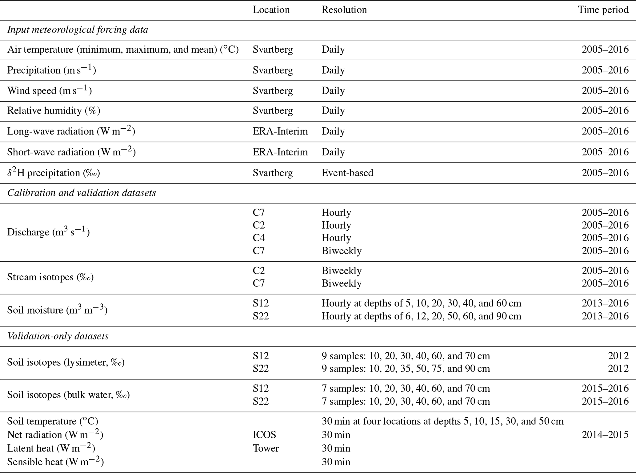
Table 1Datasets used for forcing, calibration and validation within the Svartberg catchment.
3.2.3 Soil moisture and isotope datasets
Soil moisture sensors were installed in 1997 and replaced at the beginning of 2013. The soil moisture sensors were installed at the hillslope transect location at 4, 12, 22, and 28 m locations from the C2 stream. The depths of the soil moisture measurements slightly differ between sites (Table 1); however, the depths encompass shallow and deep soil waters. Soil sensors have also been installed in the area surrounding the ICOS tower, measuring soil temperature at four locations and six depths (10, 20, 30, 40, 60, and 70 cm, Sect. S2) (Table 1) which can provide a proxy for the depth of the frost. Soil isotopes (δ2H and δ18O) were measured at multiple depths (2.5 cm increments) measured via lysimeters (2012) and bulk water samples (2015–2016).
3.3 Model set-up and calibration
All simulations were conducted on a daily time step between January 2005 and September 2016. The period from January 2005 to December 2009 was used as a spin-up period with measured hydrologic data, to stabilize δ2H, δ18O composition, and water ages in each of the model storage units. Initial analysis of the measured discharge from 2000 to 2016 revealed the highest and lowest annual discharge years were between 2010 and 2014. Consequently, calibration was carried out for the period between January 2010 and December 2014. The validation set used was the remaining period from January 2015 to September 2016. The C7 catchment was defined with a grid resolution of 25×25 m2 to balance adequate differentiation of multiple locations on the soil water transect while maintaining computational efficiency. The 25 m grid includes adjacent soil pixels for S12 and S22, with sites S04 and S28 within the same grids as S12 and S22, respectively. Within the biomass module, the vegetation dynamics for leaf growth and carbon allocation were held at steady state to minimize the parameterization and focus on the soil freeze–thaw cycles. As temperature effects and water stress are less sensitive for conifer trees, a relatively constant leaf area index and needle growth/decay rate were maintained (Liu et al., 2018). Evaporative soil water fractionation was activated using a similar parameterization to Kuppel et al. (2018b), as this has previously been identified as an influential summer process in the catchment (Ala-aho et al., 2017). Soil relative humidity was estimated using Lee and Pielke's (1992) approach, and values of kinematic diffusion were estimated as presented by Vogt (1976) (0.9877 and 0.9859 for H2∕H1 and O18∕O16 ratios, respectively). Parameterization of the model was conducted for each soil type (three soil types, Fig. 1a) and vegetation type (four types, Fig. 1b).
A sensitivity analysis established the most sensitive parameters to be used in calibration using the Morris sensitivity analysis (Soheir et al., 2014). Parameters were assessed using 10 trajectories using a radial step for evaluating the parameter space. The parameter sensitivity was evaluated using the mean absolute error. Results of this are shown in Sect. S3. Sensitive parameters were calibrated using Latin hypercube sampling (McKay et al., 1979) with 150 000 parameter sets and a Monte Carlo simulation approach to optimize the testing of the model parameter space.
3.4 Model evaluation
The model output was constrained using measurements of stream discharge (three sites, Fig. 1), stream δ2H (three sites, Fig. 1), and soil moisture (two sites, Fig. 1a). The eight measurement datasets were combined into a multi-criterion calibration objective function using the mean absolute error (MAE) with the cumulative distribution functions (CDFs) of the model goodness-of-fit (GOF) (Ala-aho et al., 2017; Kuppel et al., 2018a, b). The MAE moderated over-calibration of peak flow events, typical for functions like the root mean square error, and Nash–Sutcliffe efficiency, as well as being consistent with previous studies in the region (Ala-aho et al., 2017). To focus on the dynamics of soil moisture, given the coarse model grid, measured and simulated values were standardized by their respective mean values prior to analysis. From the CDF method, the 30 “best” simulations were selected for evaluation and are presented using a 95 % spread of predictive uncertainty (Kuppel et al., 2018b). The parameters achieved through calibration are shown in Sect. S4. Model results were verified against the remaining years of discharge, soil moisture, and streamflow δ2H, as well as independent time series of soil isotopes (bulk and lysimeter), net radiation, sensible heat, latent heat, and frost depth (estimated from depth-dependent soil temperatures).
The evaluation of changes to water ages due to soil frost was conducted by comparing the ages within the catchment for simulations of the 30 “best” parameter sets with and without frost. These were conducted without frost by turning frost dynamics off within the model. Freeze–thaw effects on evaporation and transpiration ages were evaluated as the difference between frost and non-frost simulations. Positive values indicate older water with the frost, while negative values indicate older water with frost-free simulations. The age differences were only considered on days when both frost and non-frost simulations simulate a flux greater than 0 mm d−1.
4.1 Simulation results
Calibration captured dynamics of both high- and low-flow discharge periods through both the calibration period (2010–2014) and validation period (2015–2016), with a maximum mean streamflow MAE of m3 s−1 for C7 and a maximum mean stream δ2H MAE of 5.8 ‰ at C4 (Table 2). Due to extreme high- and low-flow periods in the calibration period, it was unsurprising that the resulting MAE was higher than in the validation. The MAE of the soil moisture calibration was also reasonable, with an average MAE of 0.05 and 0.09 for sites S12 and S22, respectively. With the standardization of the soil moisture, the low MAE indicates that the dynamics in the model correspond well to those measured. The optimization of the GOF for three measures (discharge, stream δ2H, and soil moisture) at eight locations resulted in a compromise for all streams. Simulations yielded better (lower) MAE for discharge and isotopes of individual streams.
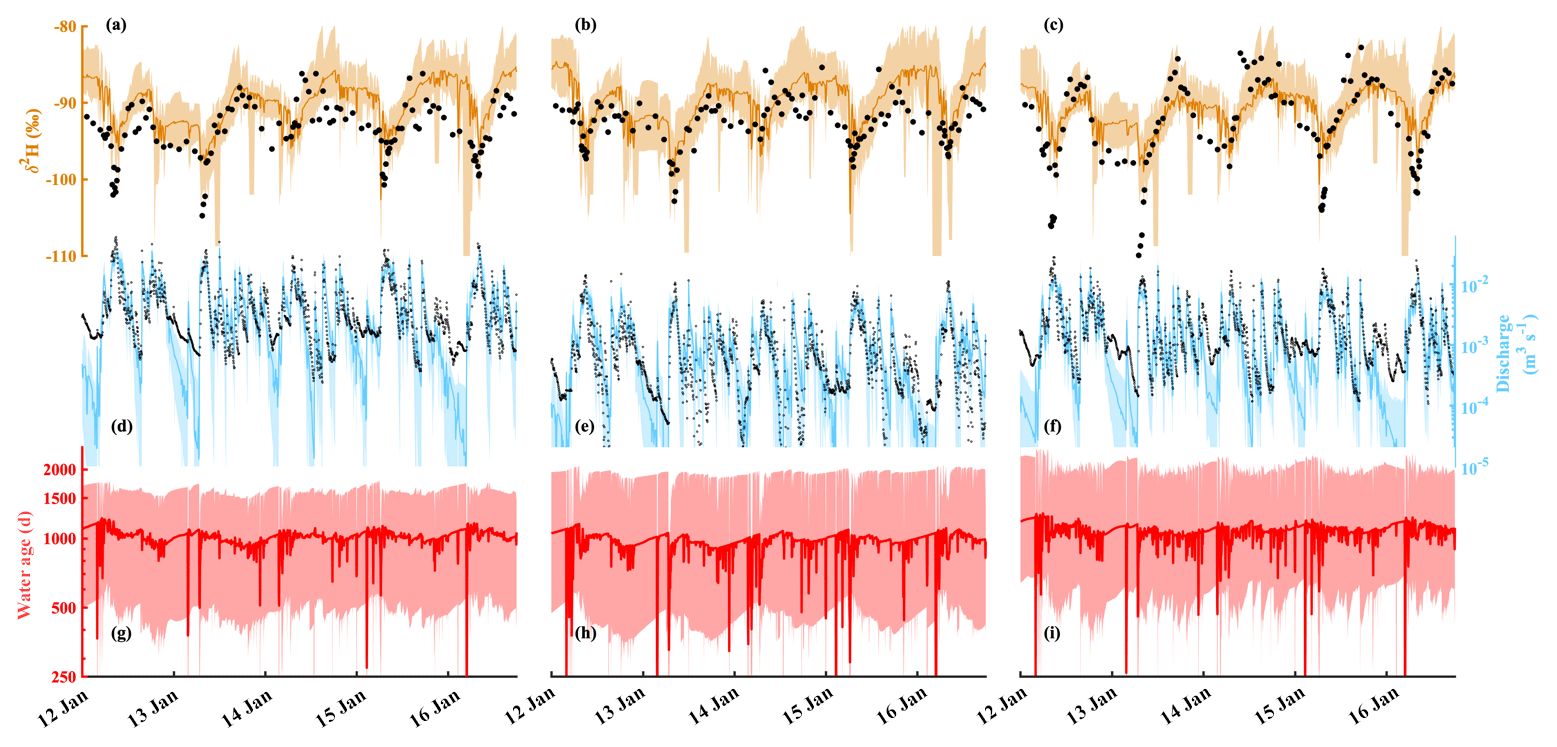
Figure 2Calibration 95 % maximum and 5 % minimum bounds, median simulation (solid line), and measured data (black circles) of δ2H for (a) C7, (b) C2, and (c) C4; discharge for (d) C7, (e) C2, and (f) C4; and stream water age for (g) C7, (h) C2, and (i) C4.
Table 2Calibration and validation efficiency criteria, shown as mean efficiency for all multi-calibration criteria.
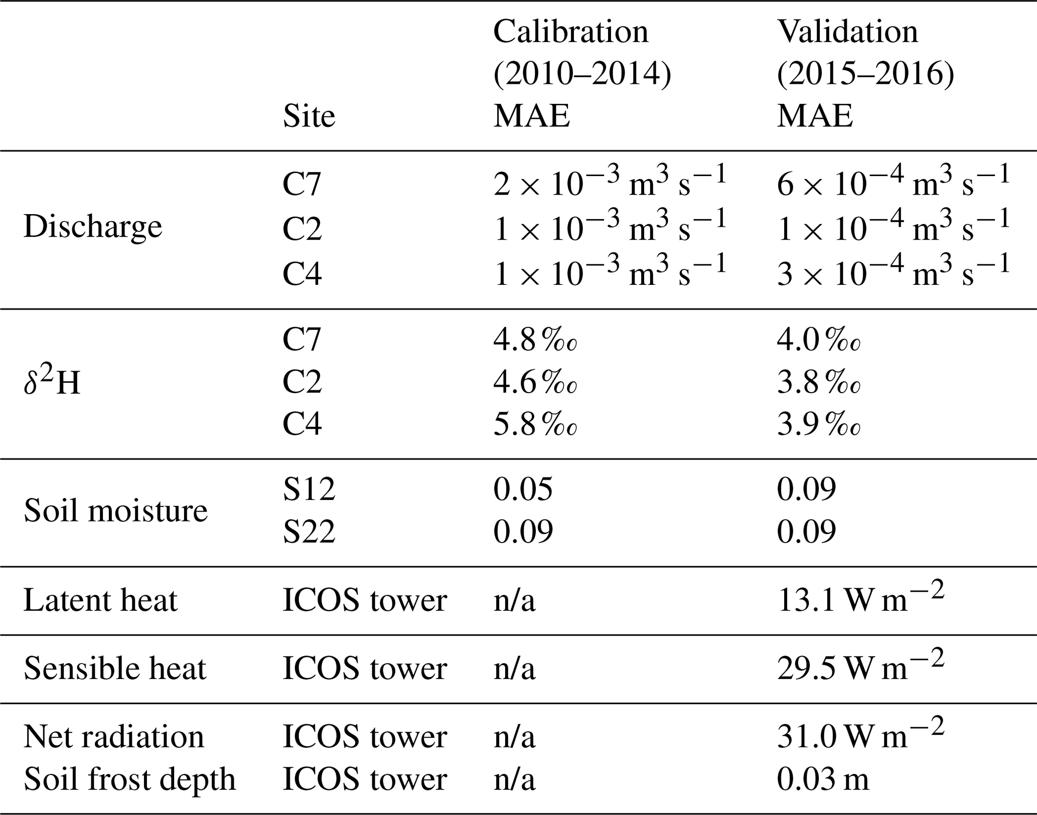
n/a = not applicable.
Temporal variability of δ2H in each of the streams was captured quite well throughout the calibration and validation periods (Fig. 2a–c). The largest offsets in modelled isotopic composition occurred during the winter low-flow conditions. The simulated stream isotopes tended to retain a slight “memory” effect from the contributions of more enriched inflow in late summer. This was likely due to the underestimation of discharge during winter (Fig. 2d–f) which slowed the flushing of the more enriched water. Overall though, discharge was adequately simulated for each site, notably during the spring melt and summer months. While flows were underestimated during the winter, the difference between simulations and measurements was typically m3 s−1. The weight-median water ages of each of the three streams were broadly similar, 2.8, 2.6, and 3.1 years for C7, C2, and C4, respectively (Fig. 2g–i). These stream ages were generally older than previous estimates, with deeper soil layers and complete mixing in each compartment tending to increase the average age. The depths of the soil layers in the peat and podzolic areas are the primary drivers of water age, with a relationship (Sect. S5). Water age decreased during the annual freshet, driven by the younger snowmelt and frozen soil water ages (typically 150–200 d old). The rapid runoff during the freshet limited the long-term influence of the younger water ages on the stream water at each of the sites as older groundwater dominated low flows. Rain-on-snow events resulted in some rapid, yet un-sustained, influences on the soil water ages, as observed with the sudden decreases in stream water age during winter months (Fig. 2g–i; log scale with a lower bound of 250 d).
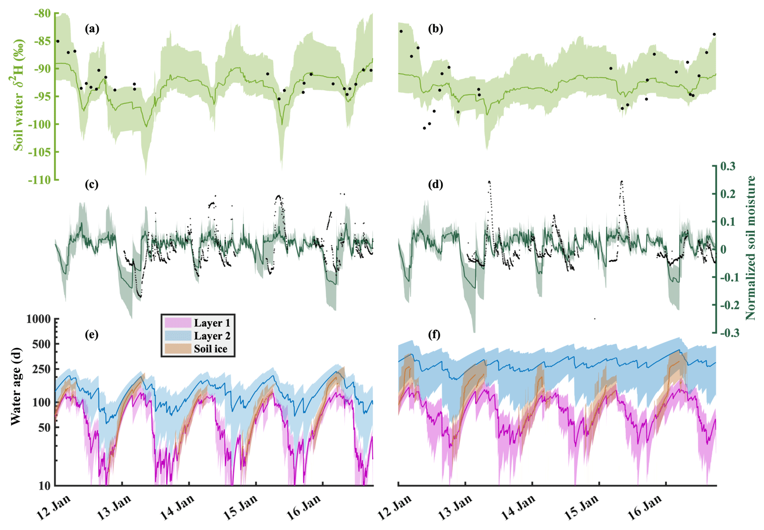
Figure 3Simulation 90 % bounds and mean simulation (solid line) for the average of layers 1 and 2 δ2H for (a) site S12 and (b) site S22; the average of layers 1 and 2 soil moisture standardized by the mean for (c) site S12 and (d) site S22; and water ages of soil layers 1 and 2 and soil frost for (e) site S12 and (f) site S22.
4.2 Soil moisture, isotope, and water ages
Simulated soil water isotopes (note that the model did not use isotopes during calibration) mostly captured those measured in both bulk water (2015–2016) and lysimeter water (2012) within the 90 % simulation bounds at the S12 and S22 sites (Fig. 3a and b). Isotope dynamics were best captured at site S12, with early season depletion due to snowmelt and enrichment of the previous summer. While most variability was captured within the 90 % bounds, the magnitude of the intra-annual contrasts at site S22 was not fully reproduced. Similar to the soil isotopes, dynamics of simulated soil moisture (calibrated) were captured at both S12 and S22, with better simulation performance at S12 (Fig. 3c and d). The model struggled to simultaneously reproduce the more damped soil moisture at S12 with the relatively dynamic soil moisture post-melt at S22 in the adjacent cell under the same soil parameterization. Rather, the same parameterization resulted in balancing of the conditions observed at S12 and S22. The large declines in measured soil moisture during the winter months were captured with the soil frost module (Fig. 3c and d). The modelled decline in the soil moisture resulted from the transition of soil water from liquid to ice. Water ages in layers 1 and 2 at each site showed noticeable intra-annual variability, and gradually declined during the growing season (May–September) and increased during the winter due to negligible water inflow (Fig. 3e and f). The gradual decrease in the soil water age during the summer was the result of younger rainfall flushing the older snowmelt and pre-winter soil water as the growing season progressed. The variability of the soil water ages in layers 1 and 2 was similar, though the ages in layer 2 were significantly older. While S12 is closer to the stream, water ages in S22 were generally older in both layers 1 and 2.
4.3 Soil freeze–thaw simulations
Simulations of frost depth revealed large inter-annual variability throughout the catchment (Fig. 4a–d), depending on winter temperatures, snowpack depth, and the soil moisture conditions. Wetter conditions in the mire generally show shallower frost depths than the podzolic soils elsewhere in the catchment. Similar soil conditions for the podzolic and thin podzolic soils (Fig. 1a) resulted in negligible differences for estimated frost depth. Overall, estimated frost depth was generally limited by the total number of freezing days. Colder winters (larger numbers of freezing degree days) resulted in deeper frost depths for an equivalent snowpack depth (e.g. Fig. 4a vs. Fig. 4c). Conversely, a deeper snowpack (higher maximum SWE) resulted in a shallower simulated frost depth for years with similar temperatures (e.g. Fig. 4a vs. Fig. 4c), as the deeper snowpack was a larger storage for incoming radiation. Using 0 ∘C in the soil temperature probes at the ICOS tower as a proxy for the depth of the soil frost, a direct comparison of simulated frost depth and the measured catchment frost depth was completed without calibration. Simulated frost depth showed good agreement with observed 0 ∘C soil temperature depth, imitating the rapid increase in frost depth in 2014 and a more gradual increase in 2015 (Fig. 4e). Late winter soil frost depth was estimated to be shallower and varied more rapidly than the observed 0 ∘C soil temperature depth (Fig. 4e). The median estimated soil depth against the measured 0 ∘C soil temperature depth showed that estimated soil thaw was too rapid, and thaw completed too early.
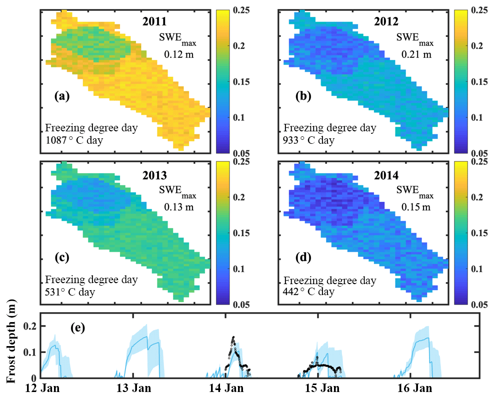
Figure 4Mean simulated soil frost depth during the peak soil frost depth in winter (a) 2010–2011, (b) 2011–2012, (c) 2012–2013, and (d) 2013–2014; 90 % uncertainty bounds of the simulated frost depth at the ICOS tower with the depth of the 0 ∘C soil temperature measured at the ICOS tower (black circles).
4.4 Evaporation and transpiration
While the evaporation, transpiration, and energy-balance datasets were not included in the calibration, modelled energy-balance components (sensible heat, latent heat, and net radiation) showed reasonable agreement with observed values in 2014–2016 at the ICOS tower. There was an underestimation of net radiation and sensible heat throughout the growing season (Fig. 5b and c) and an underestimation of latent heat late in the year (Fig. 5a). While the MAE of the latent heat was relatively small (13.1 W m−2) considering that they were not used for calibration, net radiation and sensible heat had a notable maximum bias (∼30 W m−2) during summer. Simulations of total daily evaporation (soil and interception) and transpiration had a similar pattern, with transpiration accounting, on average, for 54 % of total evapotranspiration. Throughout the year, the simulated proportion of transpiration to total evapotranspiration ranged from 31 % to 72 % except for the spring periods (Fig. 5d). The late onset of evaporation resulted from the assumption that soil evaporation was negligible while the snowpack remains, which potentially leads to an underestimation of evaporation during the melt.
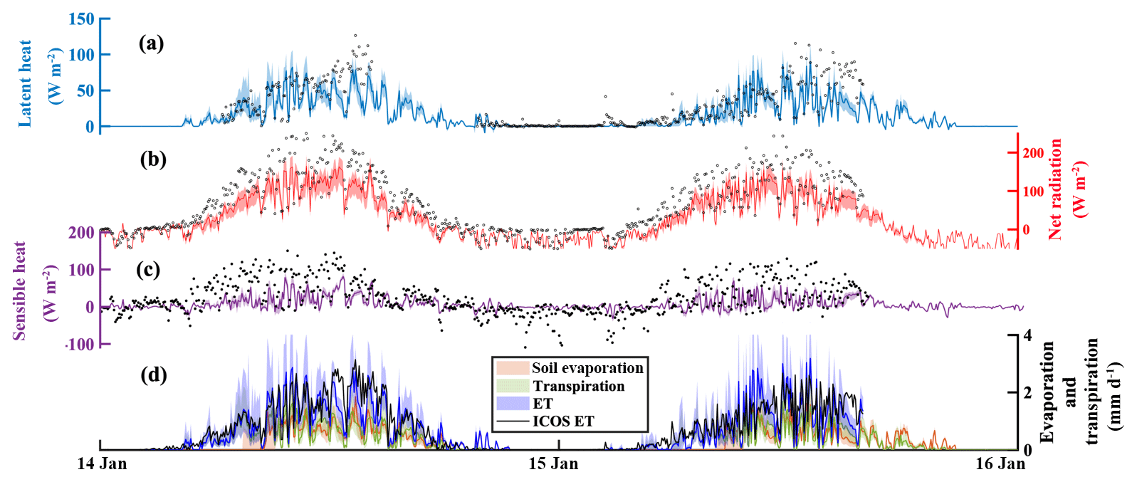
Figure 5Energy-balance component of (a) estimated latent heat (90 % and mean values), (b) estimated net radiation (90 % and median values), (c) estimated sensible heat (90 % and median values), and (d) estimated soil evaporation, transpiration, and evapotranspiration (ET) (90 % and mean values) at the ICOS tower site with the estimated total evapotranspiration from energy fluxes at the ICOS tower (black circles where data are available).

Figure 690 % bounds and median values of the (a) estimated soil evaporation water ages at the ICOS tower (blue) and in the mire (green), (b) estimated transpiration water age at the ICOS tower (blue) and in the mire (green), and (c) mean difference of evaporation and transpiration water ages when soil frost is not considered.
Ages of soil evaporation and transpiration decreased throughout the year (Fig. 6a and b), tracing the decline in soil water ages estimated with the addition of precipitation (age of 0 d). Older water present in evaporation and transpiration water at the start of the year was a mixture of the snowmelt water age and frozen water ages (from the previous summer). Spatial differences in evaporation and transpiration ages were evident throughout the catchment, shown by the difference between the forested ICOS tower site (blue, Fig. 6a and b) and the average for shrubs in the mire (green, Fig. 6a and b). The annual flux-weighted median water age of transpiration was 200±42 and 141±40 d for the ICOS tower and mire, respectively, while evaporation ages were 48±11 and 85±36 d for the ICOS tower and mire, respectively.
Differences between the evaporation and transpiration ages were determined by comparing water ages with the soil frost module activated, against those with the frost module deactivated. Generally, including frost in the simulations resulted in older water (water age difference > 0 Fig. 6c) for both evaporation and transpiration. Differences in evaporation age were not as pronounced as transpiration ages due to the slight bias of the evaporation timing (always following the snowmelt). Due to the estimated completion of soil thaw prior to the snowmelt period, the difference between the water ages of evaporation with the influence of frozen ground was modest. Rapid flushing of the soil water due to large snowmelt inputs and spring precipitation resulted in a rapid decline in the differences of transpiration water ages. Within the first month of transpiration, the difference for the frost and non-frost simulations were more notable and approached 200 d when frost limited water movement. However, the relatively lower transpiration rates, which occurred during the spring within these simulations, resulted in a moderate effect on the overall annual transpiration water ages. The effects of soil frost on stream water ages showed little effect, with negligible differences given the relatively old water bias in the stream that only shows some flashes of younger water influence (Fig. 2g–i). While the soil frost increased the stream water ages throughout the year, the effect is well within the relatively large uncertainty bounds of the stream water ages.
5.1 Modelling soil freeze–thaw processes in tracer-aided models
Hydrologic models are powerful tools for exploring the internal functioning of catchments, particularly when intensive and long-term monitoring programmes are in place to help calibration and testing (Maxwell et al., 2019). Here, the development of a spatially distributed, process-based tracer-aided model for northern climates produced encouraging results, reproducing soil frost dynamics despite the model not being directly calibrated to match frost depth observations. The use of streamflows, stream isotope ratios, and soil moisture dynamics in calibration proved to be adequate for estimating the dynamics of soil frost depth and timing of the frost onset (Fig. 4) and revealed spatial differences in frost depth due to contrasting soil types and moisture conditions. However, there are limitations with the current approach that result in some uncertainty of the effect of soil freeze–thaw on catchment hydrology. To improve the computational efficiency of the model, the temperature of the snowpack was assumed to be isothermal (Maneta and Silverman, 2013) and was modified here to include only a single temperature damping parameter. However, snowpacks may have a variable thermal gradient (e.g. Filippa et al., 2014), and are dependent on snow density (e.g. Riche and Schneebeli, 2013), snow surface albedo, wind speed, and liquid water component, among others (USACE, 1956; Meløysund et al., 2007; Sturm et al., 2010). While these additional components may contribute to an improvement in the estimation of soil frost, it likely would not have a significant improvement compared to the simple temperature damping used here with additional calibration to constrain snow water equivalent for more dynamic energy exchange (e.g. Lindström et al., 2002). The simplistic consideration of negligible soil sensible heat storage effects on the soil freeze–thaw processes, consistent with other process-based cold-region models (e.g. CHRM, Krogh and Pomeroy, 2018), may result in dampened rates of freezing and rapid melting during the spring (Kurylyk and Hayashi, 2016). More delayed melting of the soil frost may have implications for snowmelt runoff, increasing the dynamics of the streamflow isotopic compositions towards more depleted isotopic compositions (Fig. 2a–c). Finally, the simplification of a single soil frost front may have some implications for the snowmelt infiltration to the soil. The single front does not allow for near-surface soil thaw to occur prior to deeper soils and thereby has implications for shallow root-water uptake and evaporation.
Energy fluxes in northern catchments can be highly sensitive to the timing of snowmelt, yielding differences in the surface and canopy net radiation due to changing albedo, and to turbulent fluxes due to alterations in surface temperature. Here, the underestimated sensible heat flux during the spring and the growing season could be the result of many different processes. Some of these processes include the aerodynamic resistance (ra) to transpiration, an underestimated thermal gradient between the simulated soil and air temperature, an overestimation of the incoming short- or long-wave radiation from the ERA-Interim dataset, sublimation and snowpack energy storage, or an overestimation of a heat sink of ground heat through the thermal layers of the soil. An overestimated aerodynamic resistance can simultaneously reduce the transpiration (increase the surface temperature) as well as decrease the sensible heat flux (Maneta and Silverman, 2013). An overestimated surface temperature can result in both a decreased thermal gradient from the soil to the air used for the sensible heat flux estimation as well as in the shallower, and earlier, simulated soil frost melt relative to the measured 0 ∘C soil temperature depth. While the short- and long-wave radiations from the dataset had no consistent deviation from the shorter measured time series at the ICOS tower (1:1 ratio for both short- and long-wave radiation, not shown), intermittent periods of underestimated ERA-Interim radiation could contribute an underestimation of the net and sensible heat flux. Lastly, the lack of snowpack heat storage and sublimation could have an influence on the energy balance by limiting incoming winter radiation into the soils (i.e. decreasing soil temperatures).
5.2 Effect of soil freeze–thaw on water ages and implications for northern catchments
The adaptation here of a process-based, spatially distributed model to additionally incorporate fundamental cold regions processes provides the opportunity both to improve the representation of key hydrologic functions of cold catchments and to assess the effect that these processes have on transit times and ages of ecohydrological fluxes. While studies in northern catchments have aimed to assess the partitioning and transit or residence times of ecohydrologic fluxes (e.g. Sprenger et al., 2018a), few studies have included the influence of frozen conditions on the water movement. Frozen conditions may be significant for the effective transit times during the spring freshet period (Tetzlaff et al., 2018) and flowpath modelling (Laudon et al., 2007; Sterte et al., 2018). Traditionally, isotopic tracer waters at catchment outlets have been the primary metrics for assessing the water ages in streams. Here, the relatively old age of stream water and the underestimation of soil thaw result in only slightly older water ages when soil frost conditions are considered, potentially due to the smaller proportion of wetland areas (Sterte et al., 2018). The limited effect of soil frost effects on stream water age was compounded from both the wide uncertainty of the stream water ages (Fig. 2g–i) and the late deviation of soil water frost ages from the soil water (Fig. 3e and f). Generally, the uncertainty bounds of the stream water ages were greater than the difference of the soil water and soil frost ages. The smaller different of soil water and soil frost ages thereby resulted in small effective changes in stream water age. The deeper frost depth in the forested regions likely did not reduce the spring infiltration due to the low moisture content in the soil relative to the more saturated wetlands (Laudon et al., 2007). Additionally, the relatively wide uncertainty bounds of stream water age estimates present difficulties in assessing the relatively moderate effects of soil frost on the stream water age (Fig. 2). The large dependence of the flows and stream water ages at C7 on the outlet of the large mire at C4 indicates that the water age progressing through the mire will be a strong determinant of long-term change. The flux-weighted median water age estimations for the streams here were estimated to be substantially older than other tracer-aided hydrologic models for the catchment (Ala-aho et al., 2017), though they were on the upper end of other stream and hillslope transit times from transit time methods (Peralta-Tapia et al., 2016; Ameli et al., 2017). The reasons for this are largely 3-fold. Firstly, the model was calibrated with soil depths comparable to those observed in the catchment. The calibrated model used soil depths ranging from 1.5 to 6 m, where the shallower soil depths yield stream water ages comparable to previous studies. Secondly, the complete mixing assumption within the model does not allow for rapid preferential movement of young water that has been observed in numerous other recent studies (e.g. Botter et al., 2010; Harman, 2015). Incomplete mixing within the model framework would allow for deeper soil profiles to yield younger water fluxes, as estimated from isotopes alone, albeit at the expense of additional parameterization. Lastly, the previous transit time estimations (Peralta-Tapia et al., 2016; Ameli et al., 2017) do not account for older water ages of the snowpack, or the immobility and aging of frozen soil water, which would increase the estimated water ages.
Unlike stream or soil water ages, low uncertainty of transpiration and soil evaporation ages helps bring new understanding to how soil frost affects the source contributions of these ecohydrological fluxes which were the focus of the study. Ages of both transpiration and soil evaporation are consistent with soil profile modelling conducted in the region using the SWIS model (Sprenger et al., 2018b). However, the dynamics of the age variation are notably different due to the differences in the input water, where the snowmelt input to the SWIS model assumes a water age of 0 d and does not account for the “green” water fluxes during the spring months. While the transpiration ages show notable differences when frost and the corresponding discontinuity of transit times are included in the simulation, the evaporation water ages are not greatly affected. Transpiration fluxes are influenced by the frost due to the reduced liquid soil water availability and increased soil resistance to transpiration. The higher soil water deficit for transpiration does not fully restrict the transpiration flux, but reduces the fluxes until soil frost thaws and mixes the older frost water in the upper soil layers. The differences are reduced for both fluxes due to a few potential reasons. Firstly, the timing of the soil thaw has a significant influence on age estimation of soil water available for both evaporation and root uptake. While the general timing and magnitude of the soil frost depth development seems appropriately captured by the model, even without calibration, soil thaw in late winter was simulated faster than observations (Fig. 4e). There are notable differences between the ages of soil water, soil frost, and the snowpack, where soil frost is representative of the previous fall soil water, soil water is a younger water mix of the fall soil water and newer precipitation (e.g. from rain-on-snow and early spring snowmelt), and snowpack is the amount-weighted age of solid precipitation. Here, shallower soil frost and early melting of soil frost in the spring results in step-wise mixing, firstly of soil frost (oldest water, e.g. 200–300 d in Fig. 3) and soil water (moderate age, e.g. 100–125 d in Fig. 3), then of the soil water mixture and snowmelt (youngest water, e.g. 70–90 d). Since evaporation, and its corresponding age, only begins following the end of snowmelt, the greater degree of older soil frost with the younger soil water and snowmelt reduces the influence of the soil frost on the evaporation ages. Delaying the simulated timing of soil thaw would result in a larger influence of the soil water ages on both the evaporation and root uptake.
While the influence of soil frost on stream water ages was limited in this catchment, the results have potentially significant implications for modelling other catchments with frozen soils. The effect on water ages will likely be greatest in catchments where winter precipitation is limited, allowing the soil frost depth to increase from the surface, delaying the soil thaw until after the primary snowmelt. For evaporation and transpiration water ages, notable spatial differences highlight an essential consideration for northern climates in the influence of vegetation type on the source of water fluxes. In many northern areas, past glaciation results in significant wetlands typically dominated by shrub and herbaceous vegetation. Reductions in soil frost will result in greater water availability throughout the year, aiding in vegetation growth (Woo, 2013). With increased water availability throughout the year, the water use of vegetation will likely increase and thereby limit the amount of young water percolating through the rooting zone. A reduction in the amount of young water percolating through the rooting zone will likely increase the age of soil water and catchment outflows. Finally, the timing of the evaporation and root uptake needs to be strongly considered at both seasonal and diurnal timescales. Soil frost had a strong influence on the timing of evaporation and transpiration, where the magnitude of both fluxes was greater in simulations without soil frost and timing of the root uptake and soil evaporation was delayed due to ice-restricted pore spaces. While such changes are anticipated, many studies have focused on plot-scale studies, and with estimated long-term reductions of soil frost depth, larger-scale estimations of these differences are essential to understanding how catchment ecosystems will respond.
In northern environments, with a rapidly changing climate, quantitative evaluation of vegetation interactions with catchment soil water is crucial for understanding and projecting catchment responses. The process-based evaluation here of a well-monitored, long-term study catchment in the northern boreal forest region using a tracer-aided, surface–atmosphere energy-balance model has provided significant insights into the importance of soil freeze–thaw processes. Tracers were used, not only as a calibration tool, but also as validation metrics, and highlighted the effectiveness of multi-criterion calibration of a model at nested scales using discharge, isotopes, and soil moisture to constrain additional, un-measured features (e.g. soil frost depth). The progressively younger ages of evaporation and transpiration throughout the growing season show the dependence of both “green water” fluxes on spring snowmelt, which remains in soil water towards the end of the growing season. Adaptation of the EcH2O-iso model provided an opportunity to examine spatial patterns of frost depth throughout the catchment and its ecohydrological influence. Soil frost responded to both lower winter temperatures (increasing frost depths) and greater snowpack depth (decreasing frost depth). While there was little influence on the overall timing of water movement at the catchment scale as stream water ages, the greatest influence was observed within the ecohydrological partitioning, notably with the transpiration ages. Soil frost delays the onset of vegetation growth and soil evaporation, resulting in older soil water from the previous autumn to sustain early-season transpiration rather than younger snowmelt. With the implications of a reduced numbers of cold days (Guttorp and Xu, 2011) and the dependence of vegetation growth on the summer temperatures (Schöne et al., 2004) at northern latitudes, this assessment of ecohydrological partitioning is timely in understanding the effect of climatic change.
The model data are available on the Svartberget data portal (https://franklin.vfp.slu.se/, last access: December 2018) and the model code is available at https://bitbucket.org/maneta/ech2o (last access: July 2019).
The supplement related to this article is available online at: https://doi.org/10.5194/hess-23-3319-2019-supplement.
AS adapted the EcH2O-iso model from earlier work led by DT, CS, and MM, and conducted all the simulations. Data used for the model calibration and validation were collected by HL. All the authors contributed to model interpretation. AS prepared the manuscript with contributions from all the co-authors.
The authors declare that they have no conflict of interest.
This article is part of the special issue “Understanding and predicting Earth system and hydrological change in cold regions”. It is not associated with a conference.
This work was funded by the European Research Council (project GA 335910 VeWa). Marco Maneta recognizes funding for model development and applications from the US National Science Foundation (project GSS 1461576). The work in the Krycklan catchment is funded by the Swedish Research Council (SITES), SKB, Formas, and the Branch-Points KAW programme. The authors would like to recognize the University of Aberdeen IT Services, who helped with the High Performance Computing (HPC) cluster where all model simulations were conducted. Lastly, the authors thank the editor, Chris DeBeer, and the two reviewers for their suggestions which improved the manuscript, and Sylvain Kuppel for discussions regarding model development.
This research has been supported by the European Research Council (grant no. VEWA (335910)).
The publication of this article was funded by the
Open Access Fund of the Leibniz Association.
This paper was edited by Chris DeBeer and reviewed by Christopher Spence and one anonymous referee.
Ala-aho, P., Tetzlaff, D., McNamara, J. P., Laudon, H., and Soulsby, C.: Using isotopes to constrain water flux and age estimates in snow-influenced catchments using the STARR (Spatially distributed Tracer-Aided Rainfall–Runoff) model, Hydrol. Earth Syst. Sci., 21, 5089–5110, https://doi.org/10.5194/hess-21-5089-2017, 2017.
Ala-aho, P., Tetzlaff, D., McNamara, J. P., Laudon, H., Kormos, P., and Soulsby, C.: Modeling the isotopic evolution of snowpack and snowmelt: Testing a spatially distributed parsimonious approach, Water Resour. Res., 53, 5813–5830, https://doi.org/10.1002/2017WR020650, 2018.
Ameli, A. A., Beven, K., Erlandsson, M., Creed, I. F., McDonnell, J. J., and Bishop, K.: Primary weathering rates, water transit times, and concentration–discharge relations: A theoretical analysis for the critical zone, Water Resour. Res., 53, 942–960, https://doi.org/10.1002/2016WR019448, 2017.
Birkel, C. and Soulsby, C.: Advancing tracer-aided rainfall-runoff modelling: a review of progress, problems and unrealised potential, Hydrol. Process., 29, 5227–5240, https://doi.org/10.1002/hyp.10594, 2015.
Botter, G., Bertuzzo, E., and Rinaldo, A.: Transport in the hydrologic response: Travel time distributions, soil moisture dynamics, and the old water paradox, Water Resour. Res., 46, W03514, https://doi.org/10.1029/2009WR008371, 2010.
Carey, S. and Woo, M.: Freezing of Subarctic Hillslopes, Wolf Creek Basin, Yukon, Canada, Arct. Antarct. Alp. Res., 37, 1–10, 2005.
Craig, H. and Gordon, L. I.: Deuterium and oxygen 18 variations in the ocean and the marine atmosphere, in: Stable Isotopes in Oceanographic Studies and Paleotemperatures, Consiglio nazionale delle richerche, Laboratorio di geologia nucleare, Pisa, 1965.
Dee, D. P., Uppala, S. M., Simmons, A. J., Berrisford, P., Poli, P., Kobayashi, S., Andrae U., Balmaseda, A. M., Balsamo, G., Bauer, P., Bechtold, P., Beljaars, A. C. M., van de Berg, L., Bidlot, J., Bormann, N., Delsol, C., Dragani, R., Fuentes, M., Geer, A. J., Haimberger, L., Healy, S. B., Hersbach, H., Hólm, E. V., Isaksen, L., Kållberg, P., Köhler, M., Matricardi, M., McNally, A. P., Monge-Sanz, B. M., Morcrette, J. J., Park, B. K., Peubey, C., de Rosnay, P., Tavolato, C., Thépaut, J. N., and Vitart, F.: The ERA‐Interim reanalysis: configuration and performance of the data assimilation system, Q. J. Roy. Meteorol. Soc., 137, 553–597, https://doi.org/10.1002/qj.828, 2011.
Douinot, A., Tetzlaff, D., Maneta, M., Kuppel, S., Schulte-Bisping, H., and Soulsby C.: Ecohydrological modelling with EcH2O-iso to quantify forest and grassland effects on water partitioning and flux ages, Hydrol. Process., 33, 2174–2191, https://doi.org/10.1002/hyp.13480, 2019.
Fatichi, S., Pappas, C., and Ivanov, V. Y.: Modeling pant-water interactions: an ecohydrological overview from the call to the global scale, WIREs Water, 3, 327–368, https://doi.org/10.1002/wat2.1125, 2016.
Filippa, G., Maggioni, M., Zanini, E., and Freppaz, M.: Analysis of continuous snow temperature profiles from automatic weather stations in Aosta Valley (NW Italy): Uncertainties and applications, Cold Reg. Sci. Technol., 104–105, 54–62, https://doi.org/10.1016/j.coldregions.2014.04.008, 2014.
Gray, D. H. M. and Male, D. H.: Snowcover ablation and runoff, in: Handbook of snow, Pergamon Press, Willowdale, Ontario, Canada, 1981.
Guttorp, P. and Xu, J.: Climate change, trends in extremes, and model assessment for a long temperature time series from Sweden, Environmetrics, 22, 456–463, https://doi.org/10.1002/env.1099, 2011.
Harman, C. J.: Time-variable transit time distributions and transport: Theory and application to storage-dependent transport of chloride in a watershed, Water Resour. Res., 51, 1–30, https://doi.org/10.1002/2014WR015707, 2015.
Jansson, P. E.: SOIL model User's Manual: Second Edition, Swedish University of Agricultural Sciences, Department of Soil Sciences, Division of Agricultural Hydrotechnics, Uppsala, Sweden, 1998.
Jumikis, A. R.: Thermal Geotechnics, Rutgers University Press, New Brunswick, NJ, 375 pp., 1977.
Karlsen, R. H., Seibert, J., Grabs, T., Laudon, H., Blomkvist, P., and Bishop, K.: The assumption of uniform specific discharge: unsafe at any time?, Hydrol. Process., 30, 3978–3988, https://doi.org/10.1002/hyp.10877, 2016a.
Karlsen, R. H., Grabs, T., Bishop, K., Buffam, I., Laudon, H., and Seibert, J.: Landscape controls on spatiotemporal discharge variability in a boreal catchment, Water Resour. Res., 52, 6541–6556, https://doi.org/10.1002/2016WR019186, 2016b.
Krogh, S. and Pomeroy, J.: Recent changes to the hydrological cycle of an Arctic basin at the tundra-taiga transition, Hydrol. Earth Syst. Sci., 22, 3993–4014, https://doi.org/10.5194/hess-22-3993-2018, 2018.
Kundzewicz, Z. W., Mata, L. J., Arnell, N. W., Döll, P., Kabat, P., Jiménez, B., Miller, K. A., Oki, T., Sen, Z., and Shiklomanov, I. A.: Freshwater resources and their management, in: Climate change 2007: impacts, adaptation and vulnerability, Contribution of Working Group II to the Fourth Assessment Report of the Intergovernmental Panel on Climate Change, edited by: Parry, M. L., Canziani, O. F., Palutikof, J. P., van der Linden, P. J., and Hanson, C. E., Cambridge University Press, Cambridge, UK, 173–210, 2007.
Kuppel, S., Tetzlaff, D., Maneta, M. P., and Soulsby, C.: EcH2O-iso 1.0: water isotopes and age tracking in a process-based, distributed ecohydrological model, Geosci. Model Dev., 11, 3045–3069, https://doi.org/10.5194/gmd-11-3045-2018, 2018a.
Kuppel, S., Tetlzaff, D., Maneta, M. P., and Soulsby, C.: What can we learn from multi-data calibration of a process-based eco- hydrological model?, Environ. Model. Softw., 101, 301–316, https://doi.org/10.1016/j.envsoft.2018.01.001, 2018b.
Kurylyk, B. and Hayashi, M.: Improved Stefan Equation Correction Factors to Accommodate Sensible Heat Storage during Soil Freezing or Thawing, Permafrost Periglac. Process., 27, 189–203, https://doi.org/10.1002/ppp.1865, 2016.
Laudon, H. and Ottosson Löfvenius, M.: Adding snow to the picture – providing complementary winter precipitation data to the Krycklan Catchment Study database, Hydrol. Process., 30, 2413–2416, https://doi.org/10.1002/hyp.10753, 2016.
Laudon, H., Sjöblom, V., Buffam, I., Seibert, J., and Mörth, M.: The role of catchment scale and landscape characteristics for runoff generation of boreal streams, J. Hydrol., 344, 198–209, https://doi.org/10.1016/j.jhydrol.2007.07.010, 2007.
Laudon, H., Taberman, I., Ågren, A., Futter, M., Ottosson-Löfvenius, M., and Bishop, K.: The Krycklan Catchment Study – A flagship infrastructure for hydrology, biogeochemistry, and climate research in the boreal landscape, Water Resour. Res., 49, 7154–7158, https://doi.org/10.1002/wrcr.20520, 2013.
Laudon, H., Spence, C., Buttle, J., Carey, S. K., McDonnell, J. J., McNamara, J. P., Soulsby, C., and Tetzlaff, D.: Save northern high-latitude catchments, Nat. Geosci., 10, 324–325, 2018.
Lee, T. J. and Pielke, R. A.: Estimating the soil surface specific humidity, J. Appl. Meteorol., 31, 480–484, 1992.
Lindström, G., Bishop, K., and Ottosson Löfvenius, M.: Soil frost and runoff at Svartberget, northern Sweden—measurements and model analysis, Hydrol. Process., 16, 3379–3392, https://doi.org/10.1002/hyp.1106, 2002.
Liu, X., Sun, G., Mitra, B., Noormets, A., Gavazzi, M. J., Domec, J.-C., Hallema, D. W., Li, J., Fang, Y., King, J. S., and McNulty, S. G.: Drought and thinning have limited impacts on evapotranspiration in a T managed pine plantation on the southeastern United States coastal plain, Agr. Forest Meteorol., 262, 14–23, https://doi.org/10.1016/j.agrformet.2018.06.025, 2018.
Maneta, M. P. and Silverman, N. L.: A spatially distributed model to simulate water, energy, and vegetation dynamics using information from regional climate models, Earth Interact., 17, 1–44, 2013.
Maxwell, R. M., Condon, L. E., Danesh-Yazdi, M., and Bearup, L. A.: Exploring source water mixing and transient residence time distributions of outflow and evapotranspiration with an integrated hydrologic model and lagrangian partical tracking approach, Ecohydrology, 12, e2042, https://doi.org/10.1002/eco.2042, 2019.
McKay, M., Beckman, R., and Conover, W.: A Comparison of Three Methods for Selecting Values of Input Variables in the Analysis of Output from a Computer Code, Technometrics, 21, 239–245, https://doi.org/10.2307/1268522, 1979.
Meløysund, V., Leira, B., Høiseth, K. V., and Lisø, K. R.: Predicting snow density using meteorological data, Meteorol. Appl., 14, 413–423, https://doi.org/10.1002/met.40, 2007.
Pearson, R. G., Phillips, S. J., Loranty, M. M., Beck, P. S. A., Damoulas, T., Knight, S. J., and Goetz, S. J.: Shifts in Arctic vegetation and associated feedbacks under climate change, Nat. Clim. Change, 3, 673–677, 2013.
Peralta-Tapia, A., Soulsby, C., Tetzlaff, D., Sponseller, R., Bishop, K., and Laudon, H.: Hydroclimatic influences on non-stationary transit time distributions in a boreal headwater catchment, J. Hydrol., 543, 7–16, https://doi.org/10.1016/j.jhydrol.2016.01.079, 2016.
Piovano, T., Tetzlaff, D., Ala-aho, P., Buttle, J., Mitchell, C. P. J., and Soulsby, C.: Testing a spatially distributed tracer‐aided runoff model in a snow‐influenced catchment: Effects of multicriteria calibration on streamwater ages, Hydrol. Process., 32, 3089–3107, https://doi.org/10.1002/hyp.13238, 2018.
Pomeroy, J., Gray, D. M., Brown, T., Hedstrom, N. R., Quinton, W. L., Granger, R. J., and Carey, S. K.: The cold regions hydrological model: a platform for basing process representation and model structure on physical evidence, Hydrol. Process., 21, 2650–2667, https://doi.org/10.1002/hyp.6787, 2007.
Riche, R. and Schneebeli, M.: Thermal conductivity of snow measured by three independent methods and anisotropy considerations, The Cryosphere, 7, 217–227, https://doi.org/10.5194/tc-7-217-2013, 2013.
Schlesinger, W. H. and Jasechko, S.: Transpiration in the global water cycle, Agr. Forest Meteorol., 189–190, 115–117, https://doi.org/10.1016/j.agrformet.2014.01.011, 2014.
Schöne, B. R., Dunca, E., Mutvei, H., and Norlund, U.: A 217-year record of summer air temperature reconstructed from freshwater pearl mussels (M. margarifitera, Sweden), Quaternary Sci. Rev., 23, 1803–1816, https://doi.org/10.1016/j.quascirev.2004.02.017, 2004.
Soheir, H., Farges, J.-L., and Piet-Lahanier, H.: Improvement of the Representativity of the Morris Method for Air-Launch-to-Orbit Separation, IFAC Proc., 47, 7954–7959, https://doi.org/10.3182/20140824-6-ZA-1003.01968, 2014.
Sprenger, M., Tetzlaff, D., Buttle, J., Laudon, H., and Soulsby, C.: Water ages in the critical zone of long-term experimental sites in northern latitudes, Hydrol. Earth Syst. Sci., 22, 3965–3981, https://doi.org/10.5194/hess-22-3965-2018, 2018a.
Sprenger, M., Tetzlaff, D., Buttle, J., Carey, S. K., McNamara, J. P., Laudon, H., Shatilla, N. J., and Soulsby, C.: Storage, mixing and fluxes of water in the critical zone across northern environments inferred by stable isotopes of soil water, Hydrol. Process., 32, 1720–1737, https://doi.org/10.1002/hyp.13135, 2018b.
Stadnyk, T., Delavau, C., Kouwen, N., and Edwards, T. W. D.: Towards hydrological model calibration and validation: simulation of stable water isotopes using the isoWATFLOOD model, Hydrol. Process., 27, 3791–3810, 2013.
Sterte, E. J., Johansson, E., Sjöberg, Y., Karlsen, R. H., and Laudon, H.: Groundwater-surface water interactions across scales in a boreal landscape investigated using a numerical modelling approach, J. Hydrol., 560, 184–201, https://doi.org/10.1016/j.jhydrol.2018.03.011, 2018.
Sturm, M., Taras, B., Liston, G. E., Derksen, C., Jonas, T., and Lea, J.: Estimating Snow Water Equivalent Using Snow Depth Data and Climate Classes, J. Hydrometorol., 11, 1380–1394, https://doi.org/10.1175/2010JHM1202.1, 2010.
Tetzlaff, D., Buttle, J., Carey, S. K., van Huijgevoort, M. H., Laudon, H., McNamara, J. P., Mitchell, C. P., Spence, C., Gabor, R. S., and Soulsby, C.: A preliminary assessment of water partitioning and ecohydrological coupling in northern headwaters using stable isotopes and conceptual runoff models, Hydrol. Process., 29, 5153–5173, 2015.
Tetzlaff, D., Piovano, T., Ala‐Aho, P., Smith, A., Carey, S. K., Marsh, P., Wookey, P. A., Street, L. E., and Soulsby, C.: Using stable isotopes to estimate travel times in a data-sparse Arctic catchment: Challenges and possible solutions, Hydrol. Process., 32, 1936–1952, https://doi.org/10.1002/hyp.13146, 2018.
USACE – US Army Corps of Engineers: North Pacific Division: Snow Hydrology, Summary Report of the Snow Investigation, Portland, Oregon, 1956.
van Huijgevoort, M. H. J., Tetzlaff, D., Sutanudjaja, E. H., and Soulsby, C.: Using high resolution tracer data to constrain water storage, flux and age estimates in a spatially distributed rainfall-runoff model, Hydrol. Process., 30, 4761–4778, https://doi.org/10.1002/hyp.10902, 2016.
Venäläinen, A., Tuomenvirta, H., Heikinheimo, M., Kellomäki, S., Peltola, H., Strandman, H., and Väisänen, H.: Impact of climate change on soil frost under snow cover in a forested landscape, Clim. Res., 17, 63–72, 2001.
Vogt, H. J.: Isotopentrennung bei der Verdunstung von Wasser, Staatsexamensarbeit, Institut für Umweltphysik, Heidelberg, Germany, 1976.
Waite, W., Gilbert, L., Winters, W., and Mason, D.: Estimating thermal diffusivity and specific heat from needle probe thermal conductivity data, Rev. Sci. Instrum., 77, 044904, https://doi.org/10.1063/1.2194481, 2006.
Woo, M.: Impacts of climate variability and change on Canadian wetlands, Can. Water Resour. J., 17, 63–69, https://doi.org/10.4296/cwrj1701063, 2013.
Zhang, X. and Sun, S. F.: The impact of soil freezing/thawing processes on water and energy balances, Adv. Atmos. Sci., 28, 169–177, 2011.
Zhang, X., Sun, S. F., and Xue, Y. K.: Development and testing of a frozen soil parameterization for the cold region study, J. Hydrometeorol., 8, 690–701, https://doi.org/10.1175/JHM605.1, 2007.