the Creative Commons Attribution 4.0 License.
the Creative Commons Attribution 4.0 License.
 | 02 Aug 2019
Characterising spatio-temporal variability in seasonal snow cover at a regional scale from MODIS data: the Clutha Catchment, New Zealand
Todd A. N. Redpath
Pascal Sirguey
Nicolas J. Cullen
A 16-year series of daily snow-covered area (SCA) for 2000–2016 is derived from MODIS imagery to produce a regional-scale snow cover climatology for New Zealand's largest catchment, the Clutha Catchment. Filling a geographic gap in observations of seasonal snow, this record provides a basis for understanding spatio-temporal variability in seasonal snow cover and, combined with climatic data, provides insight into controls on variability. Seasonal snow cover metrics including daily SCA, mean snow cover duration (SCD), annual SCD anomaly and daily snowline elevation (SLE) were derived and assessed for temporal trends. Modes of spatial variability were characterised, whilst also preserving temporal signals by applying raster principal component analysis (rPCA) to maps of annual SCD anomaly. Sensitivity of SCD to temperature and precipitation variability was assessed in a semi-distributed way for mountain ranges across the catchment. The influence of anomalous winter air flow, as characterised by HYSPLIT back-trajectories, on SCD variability was also assessed. On average, SCA peaks in late June, at around 30 % of the catchment area, with 10 % of the catchment area sustaining snow cover for > 120 d yr−1. A persistent mid-winter reduction in SCA, prior to a second peak in August, is attributed to the prevalence of winter blocking highs in the New Zealand region. In contrast to other regions globally, no significant decrease in SCD was observed, but substantial spatial and temporal variability was present. rPCA identified six distinct modes of spatial variability, characterising 77 % of the observed variability in SCD. This analysis of SCD anomalies revealed strong spatio-temporal variability beyond that associated with topographic controls, which can result in snow cover conditions being out of phase across the catchment. Furthermore, it is demonstrated that the sensitivity of SCD to temperature and precipitation variability varies significantly across the catchment. While two large-scale climate modes, the SOI and SAM, fail to explain observed variability, specific spatial modes of SCD are favoured by anomalous airflow from the NE, E and SE. These findings illustrate the complexity of atmospheric controls on SCD within the catchment and support the need to incorporate atmospheric processes that govern variability of the energy balance, as well as the re-distribution of snow by wind in order to improve the modelling of future changes in seasonal snow.
- Article
(16113 KB) - Full-text XML
-
Supplement
(217 KB) - BibTeX
- EndNote


Globally, seasonal snow packs represent an important, yet vulnerable water resource (Barnett et al., 2005; Mankin and Diffenbaugh, 2015) and play a major role in earth–atmosphere energy exchange (Estilow et al., 2015). A decline in seasonal snow-covered area (e.g. Estilow et al., 2015; Borman et al., 2018) and shifts in the timing of snowmelt runoff have been observed in many regions of the world (e.g. McCabe and Clark, 2005; Lundquist et al., 2009; Klein et al., 2016). While most observations of reduced seasonal snow-covered area come from the Northern Hemisphere (Borman et al., 2018), negative trends have been observed over short timescales for both the alpine region of Australia (Bormann et al., 2012) and much of the South American Andes (Saavedra et al., 2018). Despite the relatively recent establishment of the Snow and Ice Network (SIN) of alpine automatic weather stations (Hendrikx and Harper, 2013), long-term records of snow occurrence and persistence are rare in New Zealand (Fitzharris et al., 1999). This scarcity of data has limited the empirical characterisation of seasonal snow processes. Subsequently, little is known about the persistence of seasonal snow across large areas of the Southern Alps / Kā Tiritiri o te Moana, the variability associated with snow persistence from year to year, and the climatic influences on such variability. Previous work to assess historical trends in snow water equivalent (SWE) in the main hydro-electric catchments of the South Island of New Zealand, which was largely model driven, revealed substantial temporal variability, but no long-term trend from the 1930s to the 1990s (Fitzharris and Garr, 1995). Conversely, modelling work undertaken to assess future impacts of climate change on seasonal snow in New Zealand predicts a substantial reduction overall in seasonal snow cover duration (SCD), the snow proportion of precipitation and peak snow accumulation through the 21st Century (Hendrikx et al., 2012; Jobst et al., 2018).
The apparent absence of any long-term trend in seasonal snow in New Zealand (Fitzharris and Garr, 1995) and the associated uncertainty resulting from a scarcity of observational data provides clear motivation for the construction of an updated observational record of seasonal snow in New Zealand's Southern Alps. The need to understand likely future scenarios of seasonal snow cover underscores the importance of such data. Remote sensing offers a means to mitigate the limitations imposed by a scarcity of in situ observations of seasonal snow, albeit over a relatively limited time span.
Remote sensing has provided substantial advances in the quantification of seasonal snow variability, with imaging sensors supporting spatial and temporal resolutions that allow a range of scales to be explored. Space-borne satellite imagers, particularly optical sensors, provide a synoptic view and have provided a step change in capability for mapping and characterising snow-covered areas, although trade-offs exist between competing resolutions (Andersen, 1982; Dozier, 1989; Nolin and Dozier, 1993; Hall et al., 2002, 2015; Rittger et al., 2013; Sirguey et al., 2009). For example, the MODerate resolution Imaging Spectroradiometer (MODIS), operating on board TERRA since 2000, and on AQUA since 2002, permits near-daily mapping of snow-covered area (SCA) at continental to global spatial scales, despite relatively coarse spatial resolution. The advance of geostationary meteorological satellites such as Himawari 8 and 9 sees comparable spatial resolution to MODIS acquired in near real time (Bessho et al., 2016). Multi-spectral sensors such as Sentinel-2A and B and Landsat 8 continue to improve the temporal resolution of imagery suitable for mapping snow at resolutions of 10–30 m (Malenovský et al., 2012; Roy et al., 2014). Passive and active microwave sensors offer the capacity to retrieve estimates of snow water equivalent directly from space-borne platforms but also suffer substantial limitations, including coarse spatial resolution in the case of passive microwave sensors, and/or complications associated with complex terrain (Lemmetyinen et al., 2018). Despite the progress in mapping SCA, reliable determination of snow depth, particularly in complex terrain, remains challenging. Modern, very high resolution stereo-capable imagers show promise for retrieving snow depth over large areas, from space, although the influence of topography on uncertainties and complications introduced by shadows in alpine terrain demand attention (Marti et al., 2016).
Although direct observation of SWE from space remains complicated, methodologies for extracting SCA from MODIS imagery can now provide relatively long records of spatio-temporal variability in SCA, itself a useful climatic indicator (Clark et al., 2009; Estilow et al., 2015). This is evidenced by the recent emergence of studies examining spatial and temporal variability in seasonal snow cover, and snow cover climatologies, across medium to large spatial scales (e.g. Gascoin et al., 2015; Saavedra et al., 2017, 2018).
This paper aims to achieve the following:
-
produce a snow cover climatology for the Clutha Catchment, New Zealand, for the years 2000–2016 – the snow cover climatology is defined here as the characterisation of the expansion and depletion of the seasonal snow cover over the course of an average hydrological year;
-
leverage the snow cover climatology to examine basin-wide temporal variability in snow-covered area and snowline elevation and assess whether any negative trend is detectable over the study period;
-
characterise spatial modes of temporal variability in snow cover duration in order to better understand spatio-temporal variability across the catchment;
-
assess the sensitivity of variability of SCD to variability in temperature, precipitation and synoptic-scale climate processes.
This is achieved by leveraging MODIS imagery to produce a 16-year time series of daily snow-covered area. While the mapping of snow-covered area from MODIS imagery is a mature approach (Hall et al., 2002; Sirguey et al., 2009; Dozier et al., 2009; Nolin, 2010; Rittger et al., 2013), characterising the spatial and temporal variability observed in the MODIS time series requires the application of robust geospatial and statistical techniques. Here, specifically the application of spatialised principal component analysis (PCA) is central to the efficient characterisation of spatio-temporal variability.
With a mean annual discharge of ∼ 530 m3 s−1 (Murray, 1975), the Clutha River drains New Zealand's largest catchment with an area of approximately 20 800 km2 (area normalised flow ∼ 800 mm yr−1). It is a watershed of primary importance to the both the Otago Region and New Zealand as a whole. Addressing the rapidly growing water needs within the Clutha Catchment presents a future challenge as demands for urban water supply and irrigation for agriculture and horticulture increase, alongside long-standing hydro-electricity commitments. Originating on the Main Divide of the Southern Alps (maximum elevation of ∼ 2800 m), much of the headwater flows are derived from rainfall and the melt of alpine snow cover, along with minor contributions from glaciers (76 km2, or 0.04 %, of the catchment is glacierised; Brunk and Sirguey, 2018). Annual precipitation totals may exceed 4000 mm on the western margin of the catchment and can be less than 400 mm in inland basins. There is no strong seasonality in precipitation. The contribution of snowmelt to the annual streamflow of the Clutha River is estimated to be 10 % by the time it reaches the Pacific Ocean (Kerr, 2013); however, this proportion is substantially higher for alpine sub-catchments and large inland basins, where it may exceed 30 %–50 %. Importantly, the spatio-temporal variability in seasonal snow within the catchment is currently not well understood. Some large tributaries arise in the semi-arid inland basins of Central Otago, where annual precipitation may be as low as 400 mm yr−1, an order of magnitude less than on the Main Divide (Macara, 2015). The Clutha Catchment includes the Dart, Rees, Shotover, Kawarau, Matukituki, Wilkin, Hunter, Nevis and Manuherikia rivers. Further references to specific catchments within this paper will be made to the Upper Clutha (Clutha up-stream of Cromwell, including lakes Wanaka and Hawea), Kawarau (west of Cromwell, including Lake Wakatipu), Lower Clutha (downstream of Cromwell) and the Manuherikia Basin, north-east of Alexandra (Fig. 1).
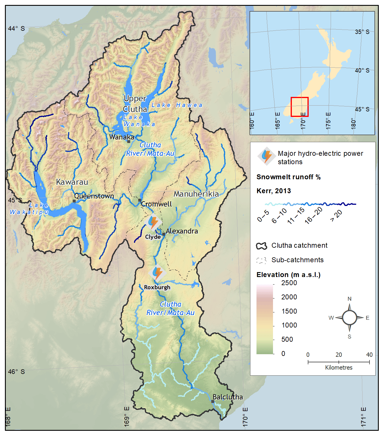
Figure 1Context map of the Clutha Catchment, including snowmelt contribution to streamflow for rivers of stream order 4 and greater, and snowmelt contribution data from Kerr (2013). The boundaries of the Upper Clutha, Kawarau and Manuherikia sub-catchments are also included. Elevation and relief data from Columbus et al. (2011); lake outlines and geographic place names are sourced from the LINZ Topographic Database and stream network and catchment boundaries from MfE River Environments Classification (Snelder et al., 2010).
Water demands within the catchment are driven by hydro-electric power generation, and irrigation. The Clutha River hosts two nationally significant hydro-electric power stations at the Clyde (432 MW) and Roxburgh (320 MW) dams, and smaller hydro-electric power stations operate on tributaries. Irrigation is particularly important in the central and eastern basins of the catchment, where climate is characterised by much lower rainfall than the mountainous regions near the Main Divide of the Southern Alps, or the coastal lower reaches of the Clutha (Murray, 1975; Hinchey et al., 1981; Macara, 2015). An important aspect of irrigation schemes in drought-prone basins such as the Manuherikia is the capture and storage of runoff generated by spring snowmelt for use later in summer (Hinchey et al., 1981). Two major local irrigation dams, the Falls Dam in the upper Manuherikia and the Fraser Dam west of Alexandra, have estimated snowmelt contributions of 15 % and 20 % respectively (Kerr, 2013). Despite a long history of hydrological research and management, the role of snow within the catchment and the impact of variability in the extent and duration of winter snow cover in the Central Otago mountain ranges have received little attention. While modelling studies indicate that significant future changes in the snow hydrology of the Clutha Catchment are likely (e.g. Poyck et al., 2011; Jobst, 2017; Jobst et al., 2018), observational studies of snow hydrology have been discontinuous and mostly limited to small sub-catchments (e.g. Fitzharris et al., 1980; Fitzharris and Grimmond, 1982; Sims and Orwin, 2011).
Seasonal snow underpins winter tourism, further contributing to the local economy (Hopkins, 2014). There are four commercial downhill ski areas, as well as a cross-country ski area, clustered in the Queenstown–Wanaka area. All ski areas have undergone expansion works in recent years, with further expansion planned. A substantial heli-ski industry is also based out of Queenstown and Wanaka. The commercial ski season typically runs from mid-June to early October; however, opening dates and season length are variable, with lifts not operating until mid-July in the “winter of discontent” of 2011 (Hopkins, 2015). Whilst modelling work suggests that the duration of natural snow packs for ski areas in Otago will be substantially reduced, and snowmaking will become increasingly important with future climate change (Hendrikx and Hreinsson, 2012), industry participants perceive inter-annual variability as having a greater impact on ski seasons (Hopkins, 2014, 2015).
Within the catchment, forest cover at elevations above 1000 m is limited. According to version 4.1 of the New Zealand Land Cover Database (Landcare Research, 2015), forest constitutes 2.84 % of the total area of 6602 km2 above 1000 m (Table S1 in the Supplement). Given the difficulties associated with recovering reliable SCA estimates from MODIS in forested areas (Raleigh et al., 2013), the low proportion of forest land cover is advantageous for the application of remote sensing techniques compared to many other mid-latitude locations.
3.1 MODIS multispectral imagery and MODImLab
MODIS is a useful sensor for mapping snow-covered area (Barnes et al., 1998; Hall et al., 2002; Sirguey et al., 2009; Painter et al., 2009; Rittger et al., 2013). In terms of spectral resolution, the SWIR bands 6 (1640 nm) and 7 (2130 nm) permit the implementation of the normalised difference snow index (NDSI) and also facilitate enhanced discrimination of snow from other targets when spectral unmixing is utilised (Sirguey et al., 2009). Additionally, global daily to near-daily re-visit times allow temporally dynamic phenomena to be captured, while also maximising the likelihood of cloud-free retrievals. Furthermore, the spatial resolution is useful for monitoring change at regional scales whereby image fusion techniques can be employed to map snow using the 250 m resolution of MODIS bands 1 and 2, offering an improvement over the native 500 m resolution of MODIS bands 3–7 (e.g. Sirguey et al., 2008).
Gascoin et al. (2015) highlighted the suitability of MODIS-derived snow cover products for characterising temporal variability in SCA and providing insight into regional snow climatology for the Pyrenees Mountains. Among several robust methodologies for mapping SCA from MODIS imagery (Masson et al., 2018), MODImLab (Sirguey et al., 2009) is used here due to its desirable capabilities and specific performance in the Southern Alps. Snow cover mapping using MODImLab for the Waitaki Catchment in New Zealand (immediately north of the Clutha Catchment) achieved a mean absolute error (MAE) < 10 % when compared with higher-resolution (15 m) ASTER reference products (Sirguey et al., 2009). Masson et al. (2018), while noting the difficulty of balancing high recall and high precision for snow mapping from MODIS imagery, found that overall MODImLab compared well with several alternatives when applied in the European Alps, Pyrenees and Moroccan Atlas Mountains.
MODImLab employs a spectral unmixing approach (in contrast to NDSI correlation applied elsewhere) to MODIS images which have undergone preprocessing, including wavelet-based image fusion to facilitate mapping of snow at 250 m resolution (Sirguey et al., 2008), and a rigorous atmospheric and topographic correction, ATOPCOR (Sirguey et al., 2009, 2016; Sirguey, 2009; Masson et al., 2018). In accounting for terrain-reflected irradiance and mitigating shadow, the topographic correction of MODImLab improves the performance of snow mapping in rugged alpine terrain (Sirguey et al., 2009; Sirguey, 2009), typical of New Zealand's Southern Alps. MODImLab operates on the basis of eight possible end-members (three being snow and one of ice), originally characterised in the New Zealand context. The pasture, rock and debris end-members are expected to align well with the land cover classes detectable within the Clutha Catchment at the MODIS scale (i.e. > 250 m) (Table S1). Re-projection of tiles from the MODIS L1B swath is handled by the swath-to-grid module within MODImLab. Imagery was resampled to a 250 m grid, in New Zealand Transverse Mercator (NZTM) projection.
3.2 Snow-covered area time series
The central process underlying this study was the construction of a continuous time series of daily, virtually cloud-free, fractional snow-covered area (fSCA) maps for the Clutha Catchment from MODIS imagery. Collection 6 (C6) MODIS/TERRA L1B swath granules were downloaded for all available observations from 1 April 2000 to 31 March 2016. Re-projection, preprocessing and mapping of fSCA was carried out using MODImLab (see full description in Sirguey et al., 2009), before implementing a cloud-filling algorithm to build the final 16-year daily cloud-free fSCA data cube used for subsequent derivation of metrics and analysis (Fig. 2). In this case, the data cube is a four-dimensional data space with two geographic dimensions (i.e. easting and northing), a temporal dimension and the fSCA dimension.
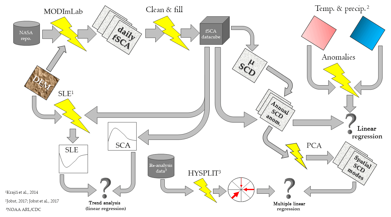
Figure 2MODIS imagery processing chain and subsequent processing (“lightning bolt” symbols) and analytical steps applied. The fractional snow-covered area (fSCA) data cube facilitates the determination of daily snowline elevation (SLE) and snow-covered area (SCA). The mean snow cover duration (μSCD) calculated over the length of the time series provides the basis for calculating annual SCD anomalies. Along with spatial SCD modes from PCA analysis these form the basis for assessing the importance of climatic forcings on spatio-temporal variability in SCD.
3.2.1 Cloud detection and gap filling
The presence of cloud, and mis-classification of cloud, or cloud shadows, as snow pixels is a common problem in multispectral remote sensing (Dozier et al., 2008). The development of a robust snow cover climatology benefits from having a cloud-free daily time series. This was achieved through the implementation of the time trajectory interpolation proposed by Dozier et al. (2008). The MOD35 cloud cover product (Frey et al., 2008) provided the basis for determining the cloud-obscured pixels for which fSCA had to be interpolated. Initially, those pixels flagged as “certain cloud” were masked. Sparse commission errors, often occurring at the edge of snow cover due to confusion between the spectral signature of cloud and mixed ground and snow pixels, were mitigated by a morphological erosion of the binary mask (Haralick et al., 1987). Two dilatations were then applied to restore the main cloud structures and conservatively extend the edges of cloudy regions. Each daily map of fSCA was combined with the associated daily cloud mask, with cloud affected pixels subsequently flagged for filling by fSCA interpolation.
Gaps resulting from cloudy pixels are then filled as proposed by Dozier et al. (2008), by applying a smoothing spline interpolant to each pixel–time trajectory. The average duration of gaps to be filled was <5 d overall, while areas of extended maximum cloud duration (>20 d) were limited to small regions of the Main Divide (Fig. 4). Implementation of the cloud-filling algorithm provided temporally continuous maps of daily fSCA. For convenience, the time series was processed into 365 d blocks, corresponding to the New Zealand hydrological year (HY, 1 April–31 March). These annual gap-filled time series provide the basis for further analysis of snow cover climatology and variability.
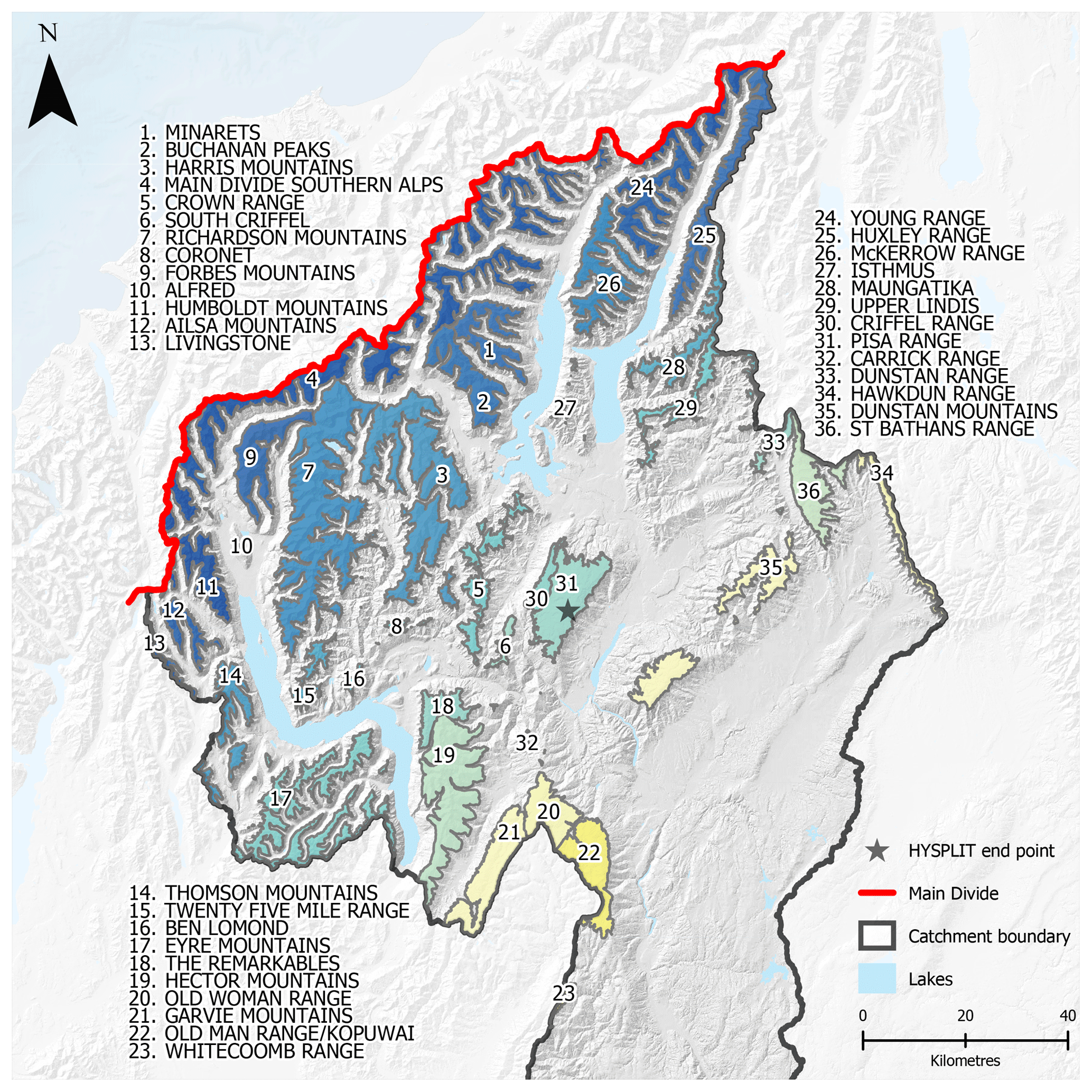
Figure 3Individual mountain ranges mapped out within the Clutha Catchment for analysis of SCD variability and temperature and precipitation sensitivity. The end point for HYSPLIT back-trajectories is also shown. Elevation and relief data from Columbus et al. (2011); lakes outlines and geographic place names are sourced from the LINZ Topographic Database.
3.3 SCD and derived metrics
The snow cover climatology can be considered initially in terms of the SCD for each hydrological year, that is, the number of days on which snow lies on the ground. SCD can be considered hypsometrically per discrete elevation bands (e.g. Gascoin et al., 2015), or spatially per pixel, as it is presented here. Spatial determination allows SCD to be mapped across the catchment. SCD was calculated as the number of days for which a pixel exceeded a minimum fSCA to avoid skewing the time series by spurious short-lived snowfall events and heavy frost detected as snow cover. In this case, the minimum threshold fSCA (fSCAt) was set to 50 %, consistent with the approach of Sirguey et al. (2009).
Calculating the SCD for each hydrological year from 2001 to 2016 (which represents the winter of the previous calendar year) also allowed the calculation and mapping of the mean (μSCD) and standard deviation (σSCD) of SCD across the catchment, over the 16-year period. In order to characterise and map associated variability, the coefficient of variation (CVSCD) was also calculated as follows:
The (CVSCD) provides an efficient means to calculate the relative dispersion of data about the mean (Brown, 1998) and has been used in other studies of spatio-temporal variability in snow cover (e.g. Hammond et al., 2018).
3.3.1 Basin snow-covered area
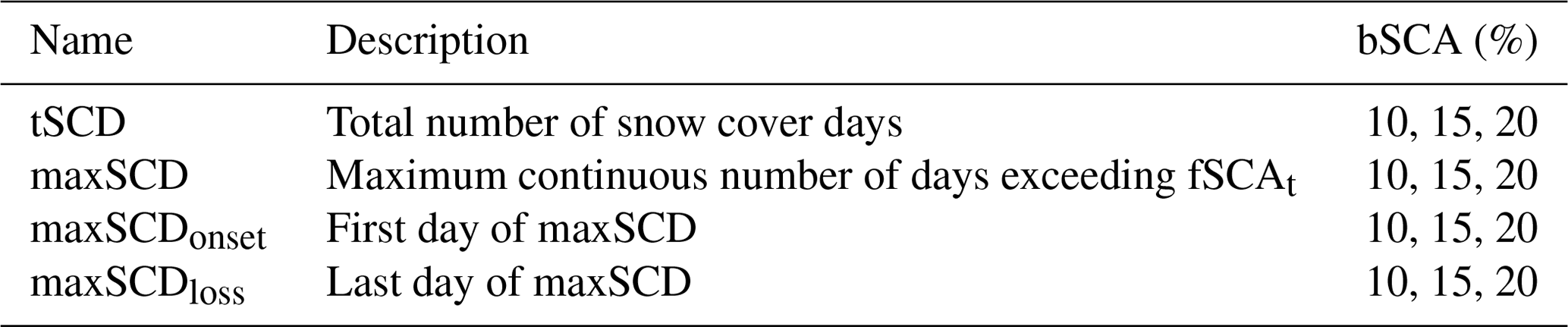
The temporal variability of snow-covered area across the basin (basin snow-covered area, bSCA) was assessed using several metrics (Table 1). These bSCA metrics were calculated as the number of days for which snow-covered pixels (fSCA ≥ fSCAt) comprised at least 10 %, 15 % and 20 % of the total catchment area. Area thresholds of 10 %, 15 % and 20 % were chosen based on basin hypsometry and informed by the mean snow-covered area. For each hydrological year, the total number of days meeting each bSCA threshold was calculated. Linear regression was applied to the annualised time series for each metric and each threshold to test the presence of any significant temporal trends.
Table 1Basin-wide snow-covered area (bSCA) temporal metrics. These metrics were calculated annually, per pixel.
3.3.2 SCD anomaly
For each hydrological year, the anomaly in SCD was calculated on a pixel-wise basis as follows:
where SCDn is the SCD map for a given year, and SCDμ is the mean SCD of all years. The magnitude of anomSCD was mapped in absolute terms. A total of 16 maps of anomSCD were derived, for the hydrological years 2001–2016 inclusive.
3.3.3 Snowline elevation
The snow line elevation (SLE), which may be defined as the minimum elevation at which relatively contiguous snow cover is present within a landscape, is a useful metric for characterising the state of seasonal snow at a point in time (Krajčí et al., 2014; Drolon et al., 2016). In simple terms, the occurrence of snowfall and the development of a snowpack is expected to be governed by temperature and precipitation, and this often generally results in a well defined snowline in New Zealand (Barringer, 1989). The method developed by Krajčí et al. (2014) was implemented on the gap-filled time series to determine daily SLE from fSCA maps and a corresponding digital elevation model (DEM). Deriving snow line elevation is an iterative process, where for a test elevation (zi) the number of snow-covered pixels (PS) below, and the number of snow-free pixels (PL) above is minimised. This is determined by calculating an F value for each test elevation as follows (Krajčí et al., 2014):
In the case of the Clutha Catchment, F(z) is calculated from 300 to 2700 m at 10 m increments. Elevation data were sourced from the NZSoSDEM, a freely available 15 m resolution DEM (Columbus et al., 2011), resampled to 250 m to match with the fSCA maps. SLE was determined using the 16-year gap-filled time series derived from MODImLab fSCA products. Pixels were considered snow-covered for the purpose of deriving SLE when pixel fSCA ≥ fSCAt.
3.4 Characterising spatio-temporal variability
3.4.1 Spatialised principal component analysis
Principal component analysis reduces the dimensionality of multivariate datasets by determining linear combinations of variables that provide a number of de-correlated principal components (PCs), each characterising a proportion of the total variance in the underlying data (Dunteman, 1989; Jackson, 1991). This approach has a long history of use in climatological research for characterising spatial patterns in the distribution of key parameters such as temperature, precipitation and atmospheric pressure (Tait et al., 1997); sea ice concentration (Baba and Renwick, 2017); and ice shelf behaviour (Campbell et al., 2017). In these applications, PCA typically reveals the spatial structure of important, and often persistent, features within spatially distributed observations. The temporal component of variability, however, may not be readily interpreted from this “atmospheric science PCA” (Demšar et al., 2012).
When applied to spatio-temporal data, such as time series of raster maps capturing a spatially continuous variable, each principal component is a map representing a spatial mode of variability occurring within the time series. The PCs are ordered according to the proportion of overall variance they explain. Conceptually, this approach, which can be considered as “raster PCA” (rPCA) (Demšar et al., 2012) is analogous to the application of PCA to multispectral imagery, where PCs are determined in a temporal, rather than spectral, attribute space. Spatialisation is a product of the geo-referenced raster datasets, and PCs are calculated only in the attribute space, so geographic effects are not accounted for (Demšar et al., 2012). A key benefit of the rPCA approach is that, when applied to a raster time series, it allows the occurrence of specific modes of spatial variability to be considered as a function of time. Thus, the spatio-temporal variability within the data is preserved and can be further scrutinised and interpreted.
Here, rPCA was applied to the time series of SCD anomaly maps. The resulting PCs provide an indication of the spatial and temporal variability in the SCD anomaly. PCA was carried out using MATLAB®. The single value decomposition algorithm was applied to the time series of 16 SCD anomaly maps, yielding as many PCs. The first six PCs were retained as together they explained > 75 % of the total observed variance, while the remaining PCs become increasingly less spatially coherent and are of limited use for further analysis and interpretation.
3.4.2 Temporal dynamics of spatial modes
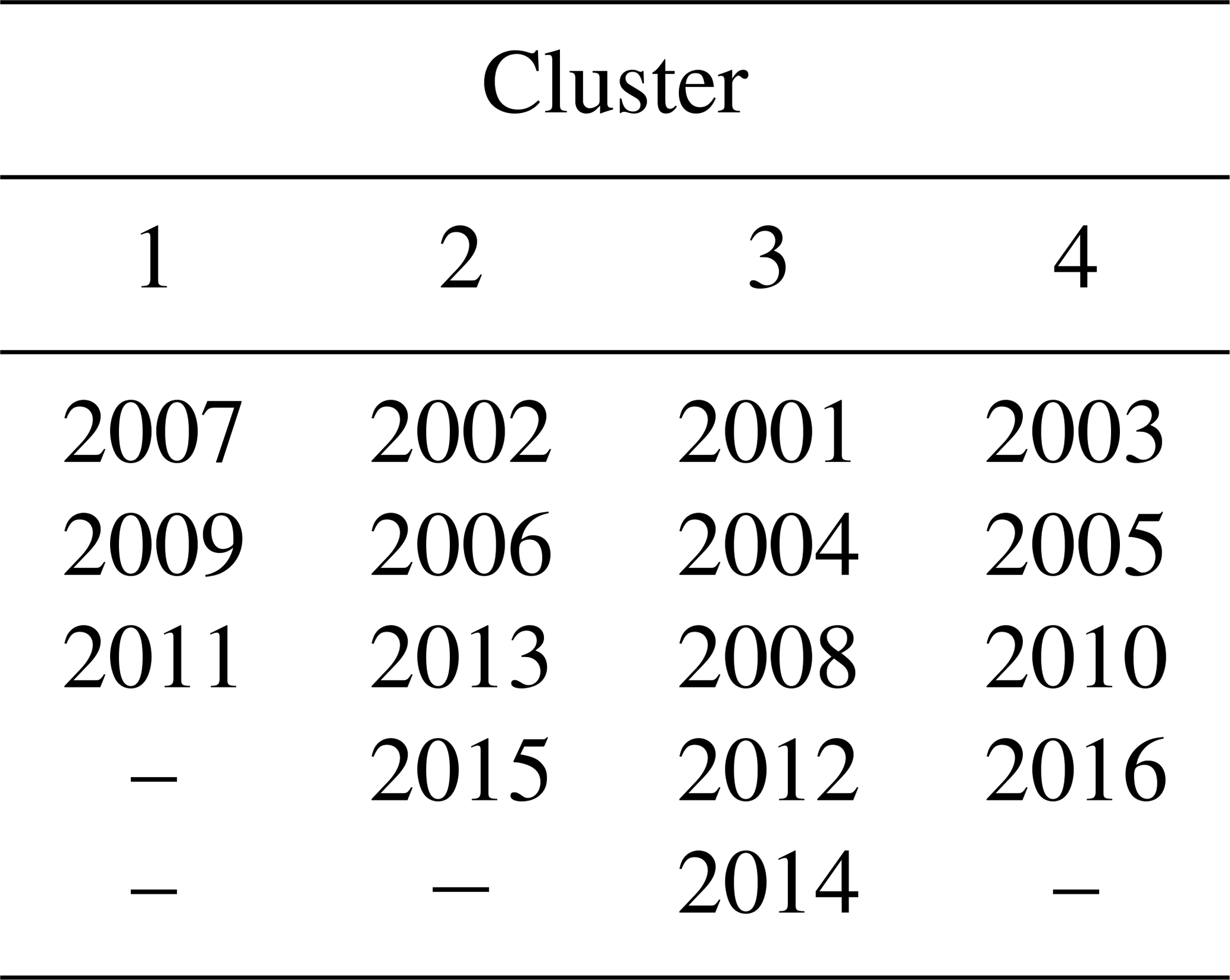
Each PC from the rPCA described in Sect. 3.4.1 reveals spatial modes of variability. In turn, the respective loadings of each PC can be used to identify years which share similarities in the spatial expression of their SCD anomalies. Comparing years based on their PCA signatures was done by considering the loadings of the first six PCs, which explained 77 % of the total variance in the spatio-temporal dataset. The PCA provided a six-dimensional loading space, within which the similarity between years was measured by the Euclidean distance and k-mean clustering.
3.4.3 Mountain range analysis
An alternative, semi-distributed approach was considered for characterising spatial variability in SCD. Addressing space via individual mountain ranges provided a basis to explore spatial gradients in SCD variability across the catchment. This approach allows the catchment to be treated in a way that may be more readily understood by stakeholders, potentially including industrial and agricultural water managers and consumers, ski area operators, and the general public. Such stakeholders typically consider the snow resource at a sub-catchment mountain range scale. The goal of this analysis was to determine whether mountain ranges provide a useful geographic unit for capturing and characterising spatial variability. The catchment was subdivided into 36 different mountain ranges, based on the naming conventions provided by the 1:50 000 scale NZ Geographic Names topographic dataset (LINZ, 2017). All land areas below the median winter snow line elevation (as calculated in Sect. 3.3.3) of 1270 m were excluded. Then, areas of mountain ranges above this elevation were manually digitised using a DEM (Columbus et al., 2011) and stream centre-line vector data (Snelder et al., 2010) as guidance (Fig. 3). Since the Main Divide of the Southern Alps is considered to provide a baseline for climatic gradients in the east of the South Island, owing to predominant westerly air flow and the substantial orographic effects of the Southern Alps (Sinclair et al., 1997; Jobst et al., 2018), the distance from each range to the Main Divide of the Southern Alps was calculated using the Near tool in ArcGIS v10.3. Mean annual SCD anomalies for each range were then extracted from the maps calculated in Sect. 3.3.2. Ranking each range in terms of proximity to the Main Divide then provided a basis for examining spatial trends in the SCD anomaly across the catchment from year to year.

Figure 4Maps of the mean duration of cloud occurrence (a), mean of the maximum annual cloud occurrence duration (b) and histograms of both (c). Lake outlines are sourced from the LINZ Topographic Database.
3.5 Climatic influences on snow cover variability
Beyond characterising the snow climatology for the Clutha Catchment, relating spatio-temporal variability in SCD to climatic variability is central to better understanding climatic influences on seasonal snow in New Zealand. This was done firstly by assessing the sensitivity of the annual SCD anomalies to annual temperature and precipitation anomalies. Furthermore, the role of atmospheric circulation was assessed by considering airflow as characterised by multiple atmospheric back-trajectories generated for the study period using the Hybrid Single-Particle Lagrangian Integrated Trajectory (HYSPLIT) model (Stein et al., 2015). Airflow analysis was motivated in part by the suggestion that increased frequency of southerly airflow can significantly suppress temperatures in New Zealand (Dean and Stott, 2009), but also because variability in airflow can be expected to produce spatial variability in the delivery of precipitation to the Clutha Catchment.
Several climatic datasets were acquired to investigate the role and relative influence of climatological processes in controlling the variability of seasonal snow, namely the following:
-
Gridded temperature and precipitation fields, comprising daily Tmax, Tmin, Tmean and Ptot for the period 2000–2016, interpolated at a resolution of 250 m, coincident with the pixel size of comparable MODIS datasets, produced as detailed in Jobst et al. (2017) and Jobst (2017). In the case of temperature, gridded data were produced from a limited observational network using a trivariate spline that was enhanced using process-driven lapse rate models (Jobst et al., 2017). Precipitation was also interpolated using a trivariate spline, with a 30-year normal surface included as a covariate (Jobst, 2017).
-
Monthly values of the Southern Oscillation Index (SOI), and Southern Annular Mode (SAM, also known as the Antarctic Oscillation Index, AAO), from the NOAA National Weather Service Climate Prediction Center (CPC). Data were sourced from https://www.cpc.ncep.noaa.gov/products/precip/CWlink/daily_ao_index/aao/aao_index.html (last access: 27 July 2017) (SAM) and https://www.cpc.ncep.noaa.gov/data/indices/soi (last access: 28 June 2017) (SOI).
-
Global gridded (2.5∘) NCEP/NCAR meteorological reanalysis data (Kalnay et al., 1996), used as input fields for the HYSPLIT (version 4) model. Data were acquired from the Climate Data Center (CDC) via the FTP module within the HYSPLIT software.
3.5.1 Spatial anomalies for temperature and precipitation
The daily fields of mean temperature and total precipitation described above were used to calculate pixel-wise mean values for each hydrological year, as well as for each winter period. Winter was defined as being from 1 May to 30 October, the period during which the majority of substantial snowfall events occur. Pixel-wise anomalies in annual mean temperature and total precipitation were calculated to produce a series of 16 anomaly maps for each variable, which were compared directly with the SCD anomaly maps. No significant correlation existed between temperature and precipitation anomalies.
The sensitivity of SCD anomalies to temperature and precipitation anomalies was assessed in a semi-spatially distributed way. Regression analysis was carried out between the annual SCD anomaly and temperature and precipitation anomalies averaged over each mountain range. Sensitivity of SCD to temperature and precipitation variability could then be quantified and its significance assessed for each mountain range across the catchment.
3.5.2 Synoptic-scale airflow variability
HYSPLIT is a Lagrangian air parcel trajectory and dispersion model (Stein et al., 2015). While it offers complex simulations of particle atmospheric transport, dispersion, chemical transformation and deposition, the trajectories modelled by HYSPLIT provide a means to characterise airflow and associated air-mass characteristics. Here, HYSPLIT was used to determine and analyse the origin and trajectory of air parcels arriving to the Clutha Catchment throughout the study period.
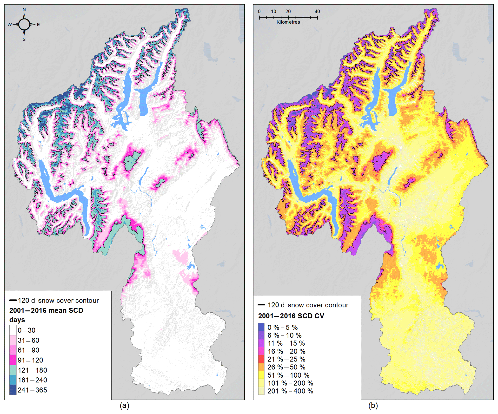
Figure 5Mean annual SCD (μSCD) (a), and associated coefficient of variation, CV (CVSCD) (b), for the Clutha Catchment, 2001–2016. Elevation and relief data from Columbus et al. (2011); lake outlines are sourced from the LINZ Topographic Database.
The geographic end-point for the trajectories was a location near the summit of the Pisa Range (Fig. 3), with elevation set to 2000 m. This location was close to the geographic centre of the Clutha Catchment (−44.90∘ S, 169.16∘ E; Fig. 3) and therefore expected to provide a suitable characterisation of modes of air flow affecting the catchment throughout the year. Back-trajectories were calculated over 120 h for each day of the study period, with four temporal end-points per day (00:00, 06:00, 12:00, 18:00 New Zealand Standard time, NZST). In total this provided 1460 trajectories per year.
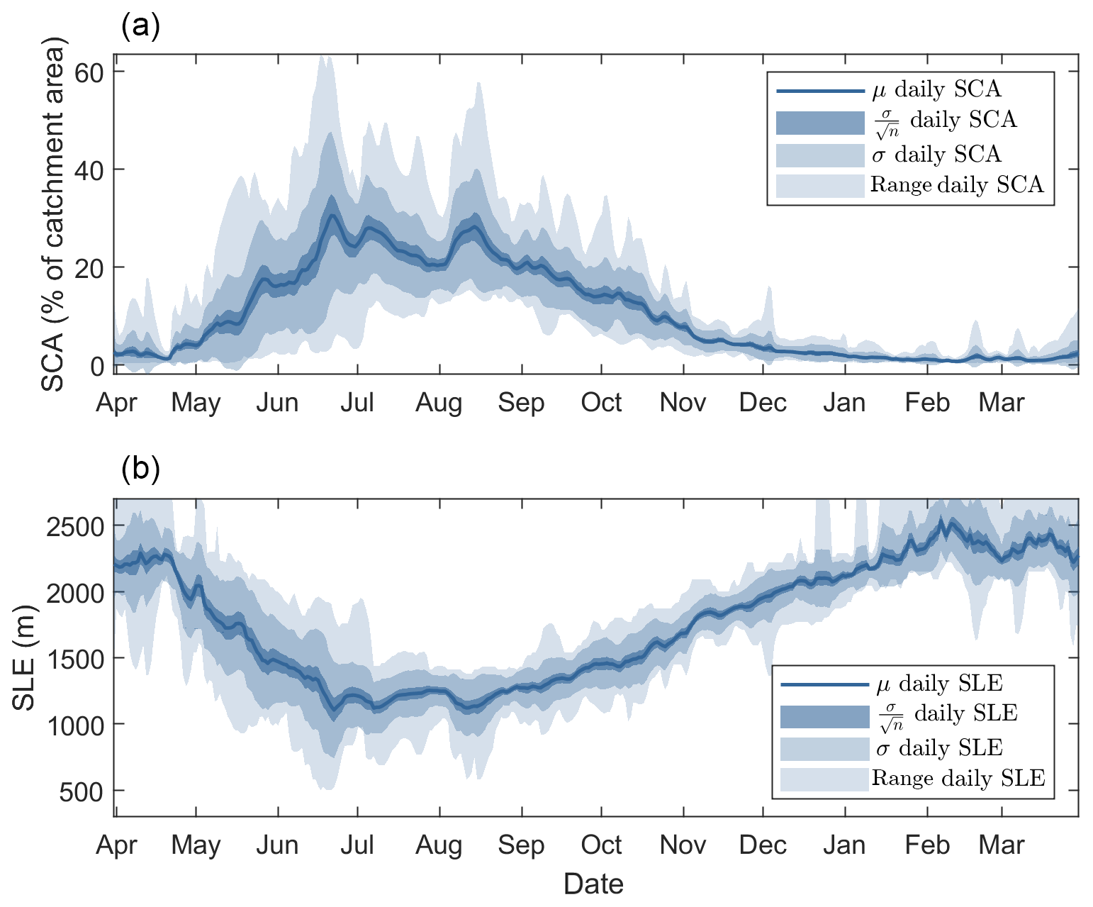
Figure 6A 10 d moving average of daily snow-covered area (SCA) (a) and snowline elevation (SLE) (b). The mean of each is shown in black, accompanied by the envelopes of associated standard deviation and range (illustrating the spread of trajectories), as well as the standard error (representative of the uncertainty of the mean).
HYSPLIT trajectories were used to construct indices of air-mass origin. For four timesteps, namely −96, −72, −48 and −24 h, the trajectory direction relative to the end-point was determined and binned according to eight directional classes (i.e. N, NE, E, SE, S, SW, W, NW). This allowed the mean frequencies of air parcel origin direction and relative frequencies for each winter (1 June–30 September) period to be calculated. The relative frequency distribution for each winter then provided a means to characterise air-flow characteristics for each winter.
Relationships between the annual loadings of each principal component of SCD and the relative frequency of air parcel origin direction were assessed by multiple linear regression. Because of the large number of variables (8) relative to the number of years for which data exist (16), only four directions exhibiting the greatest inter-annual variability were included in multiple linear regression to mitigate against under-determination. This means that, for each principal component (n) and each year (y), the linear model took the following form:
where λn(y) is the loading of the nth PC for that year, and and are the SCD sensitivity to and relative frequency of air parcels originating in the NE, E, SE and S. This analysis allowed the contribution, importance and significance of anomalous airflow directions to the modes of spatial variability in SCD to be assessed.
3.5.3 Assessing the role of climate modes
Commonly, short- to medium-term variability in climate and cryospheric processes in mid-latitude regions has been considered in terms of large-scale climate modes such as the SOI, the SAM and the Pacific Decadal Oscillation (PDO) (e.g. McKerchar et al., 1998; Fitzharris et al., 2007; Kidston et al., 2009; Purdie et al., 2011; Sirguey et al., 2016). Periods of negative SOI phase are expected to correspond with cooler periods of increased solid precipitation in New Zealand, and have been associated with positive mass balance for glaciers in the Southern Alps (McKerchar et al., 1998; Lamont et al., 1999; Fitzharris et al., 2007; Purdie et al., 2011), yet its inclusion as a predictor variable does not necessarily increase the skill of hydrological forecast models (Purdie and Bardsley, 2010). Here, mean winter values of the SOI and SAM indices were compared to each of the temporal metrics characterising snow cover within the catchment (Table 1) via correlation analysis and linear regression. The PCA analysis proposed by this study provides new insights into the spatial expression of snow cover variability that also deserves further scrutiny. Subsequently, the influence of large-scale circulation indices on spatial modes of snow cover was explored by analysing the correlation between the SOI and SAM and annual PC loadings.
4.1 Snow cover climatology for the Clutha Catchment
The snow cover climatology for the Clutha Catchment is expressed spatially by the map of μSCD over the period 2000–2016. The first-order control of elevation on SCD is obvious in Fig. 5a. On average, an area of 2218 km2, or 10 % of the total catchment area, maintains snow cover for 120 d a year or more. In general, snow cover is most persistent on terrain above 1500 m a.s.l., and on slopes with a southern aspect.
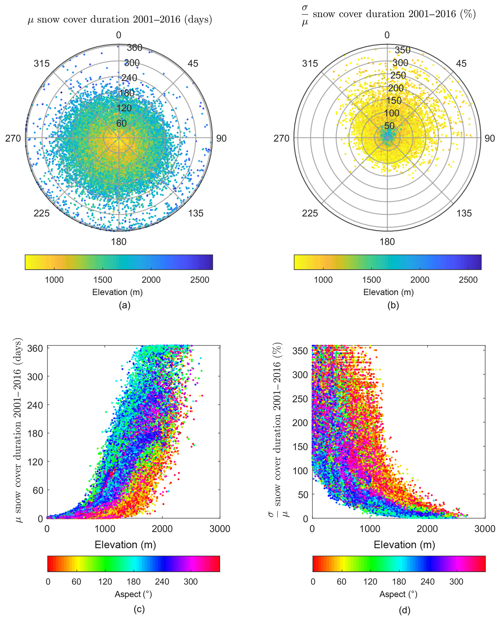
Figure 7Mean SCD (a, c) and associated coefficient of variability () (b, d) as a function of aspect (a, b), and elevation (c, d). For clarity, a random sub-sample of 50 000 pixels is displayed in the plots.
The mean SLE during the winter period was found to be 1263 m a.s.l; this corresponds with an area of 3180 km2 and is substantially higher than the mean catchment elevation of 615 m. On average, the snowline is at or below this elevation from mid-June until mid-August (Fig. 6). A small area of 76 km2 maintains permanent snow cover (SCD > 360 d). This corresponds with a maximum SLE of around 2200 m a.s.l. Considering the detection limits of MODIS, this area agrees well with the glacier area of Brunk and Sirguey (2018). These areas are largely restricted to within a few kilometres of the Main Divide. The importance of aspect in maintaining permanent snow cover for these high-elevation regions is highlighted in Fig. 6.
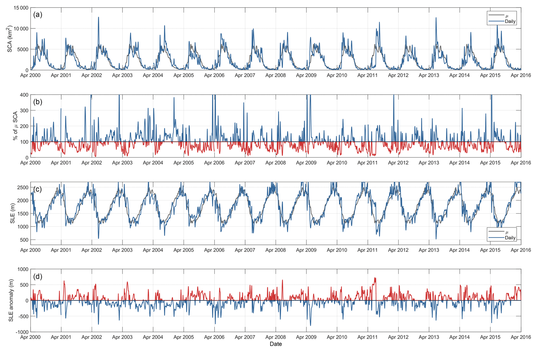
Figure 8A 5 d moving average of daily snow-covered area (SCA) and percentage of mean snow-covered area for all years (a, b), and daily snowline elevation (SLE) and daily SLE anomaly (c, d). Mean daily values, repeated for each year, are shown in grey in the daily SCA and SLE plots.
The onset of the snow season is typically rapid, with SCA increasing and SLE lowering abruptly in the early winter, reaching their maximum and minimum, respectively, in mid-June (Fig. 6). At the catchment scale, both SCA and SLE feature a mid-winter depletion and rising respectively, before SCA increases and SLE decreases again in late winter to early spring. Maximum SCA typically reaches > 35 % of the catchment area during June, yet the depletion curve is punctuated by local maxima. On average, the first of these occurs in early July, and the second in mid-August. These features are persistent throughout the 16-year study period. In addition, a minima in variability of daily SCA occurs in late April, following an increase in variability due to early snowfall over the preceding month. Variability in basin SCA and SLE is greatest during the May–July period and converges towards the mean through spring and early summer.
4.2 Topographic controls on snow duration and variability
Figure 7 shows the overall control of aspect and elevation on SCD and its variability. Most pixels exhibiting μSCD > 120 d have a southerly aspect between 90 and 315∘ and elevation in excess of 1500 m. The role of aspect strengthens as elevation decreases. The variability in SCD is more pronounced on northerly aspects between 315 and 90∘, across all elevations. In contrast, the CVSCD rarely exceeds 100 % for pixels with S to SW aspect between 135 and 270∘, but may exceed 200 % for pixels with northerly aspect between 315 and 90∘ (Fig. 7).
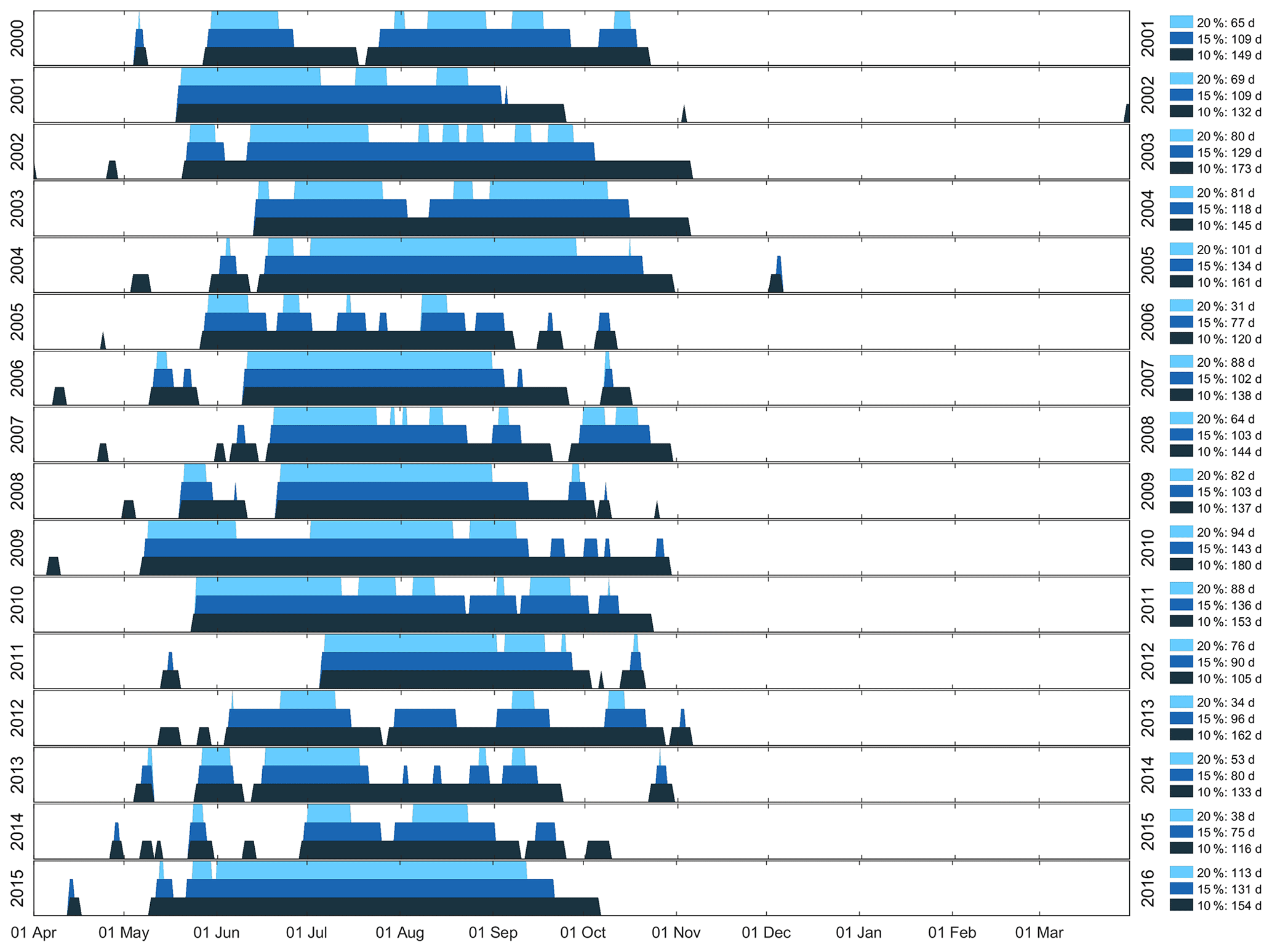
Figure 9Timeline of occurrence of 10 %, 15 % and 20 % basin snow-covered area (bSCA) for the Clutha Catchment for hydrological years 2001–2016.
μSCD is positively, though not linearly, correlated with elevation. The rate of increase of μSCD with elevation is higher on southerly than northerly aspects (Fig. 7). A CVSCD < 10 % is generally restricted to southerly aspects above 1500 m. Elsewhere, variability in SCD is relatively large. CVSCD increases markedly at lower elevations reflecting the relatively short μSCD and associated large inter-annual variability.
4.3 Spatio-temporal variability in seasonal snow cover
The map of CVSCD shown in Fig. 5b highlights the magnitude of spatio-temporal variability associated with SCD in the Clutha Catchment. A first-order control of elevation on CVSCD is apparent, but further spatial variation exists beyond the basin hypsometry. Areas with CVSCD ≤ 5 % were only present on and near the Main Divide, while CVSCD is much greater elsewhere in the catchment. At moderate to high elevations, CVSCD in the western part of the catchment was generally less than 50 %. In the eastern part of the catchment, CVSCD was generally greater, but this reflects the basin hypsometry to an extent. Ultimately, the large CVSCD observed across most of the catchment reflects the temporally dynamic nature of snow cover across the Clutha Catchment.
4.3.1 Temporal variability in catchment-wide snow cover and snowline elevation
The full time series of daily SCA and SLE and associated departures from their series means reveal the extent of temporal variability in seasonal snow at the catchment scale (Fig. 8). Substantial departures from the mean throughout the time series highlight the strong inter-annual as well as shorter-term variability in the occurrence, persistence and disappearance of seasonal snow within the catchment. Large, yet short-lived, perturbations occur due to unseasonable snow events, while sustained positive and negative anomalies occur at seasonal scales during winter. The maximum observed SCA was 65 % and occurred on 18 June 2002. The only other occasion on which SCA exceeded 60 % of catchment area was 21 June 2013. Notably, the years that feature the largest maximum SCA values are not always associated with a sustained positive anomaly in catchment-wide SCA.
The considerable temporal variability associated with SCA is further demonstrated by the bSCA metrics plotted in Fig. 9. The total number of days each year with bSCA exceeding 10 %, 15 % and 20 % is highly variable from year to year and did not reveal any significant trend over the 16-year time series. The lowest returned p value (0.23) was associated with a negative trend for the end date of temporally continuous 15 % bSCA. Typically, 10 % bSCA is achieved by June, with the latest onset date of 6 July occurring for HY 2012. Generally, 10 % bSCA is sustained through 30 September, resulting in a mean 120 d duration. The earliest end date for 10 % bSCA, 8 September, occurred for HY 2006. Several years saw 10 % bSCA extend through, or beyond, 31 October. For HY 2010, an early onset of continuous 10 % bSCA (7 May), combined with a loss date of 30 September, resulted in the longest continuous duration of 10 % bSCA, of 176 d.
Both 15 % and 20 % bSCA saw much more variability, with the period of 20 % bSCA being discontinuous for most winters. Onset of both 15 % and 20 % bSCA typically occurred within a few days of 10 % bSCA; however, there was usually considerable lag between the end date of 15 % and 20 % bSCA and that of 10 % bSCA.
The winter SLE also exhibited significant intra- and inter-annual variability, both in terms of the mean (median) winter SLE of 1263 m (1270 m), and the range of observed SLE (Figs. 8 and 10). The largest ranges of observed winter SLE (e.g. HY 2012), were associated with years when the onset of winter snow cover was delayed. This scenario reflects an over-representation of high SLE through June, which is the month when the lowest SLE values are usually observed across the entire record. Similarly to SCA, no significant temporal trend was detected in SLE over the 16-year record.
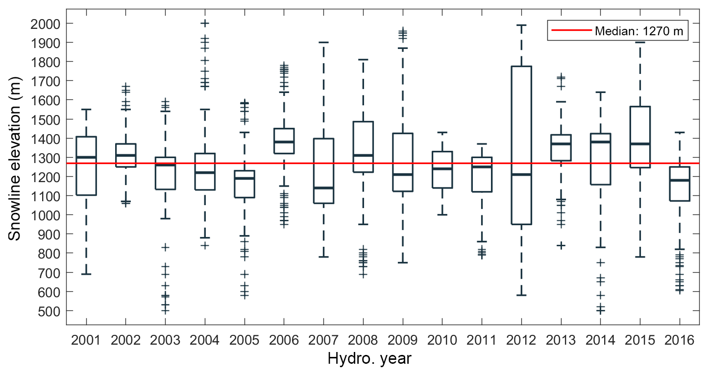
Figure 10Box plots of winter (1 June–30 September) snowline elevation for all years. The upper and lower bounds of the boxes are the 75th and 25th percentiles, respectively. Outliers are represented by “+” symbols.
4.3.2 Modes of spatial variability
Mapping the principal components of the SCD anomaly revealed distinct modes of spatial variability (Fig. 11). 77 % of the total observed spatial variability in the annual SCD anomaly was explained by the first six principal components (Fig. S1 in the Supplement). In turn, each annual SCD anomaly map can be efficiently reconstructed via linear combination of each map of PC scores. As such, the loadings of the combination quantify the relative contribution of each mode to the SCD map. Since PC scores are not standardised, their unit matches that of the SCD anomaly (i.e. day). Where loadings are positive (negative), a positive PC score will propagate positively (negatively) into the SCD anomaly. PC1 (39 % of total variability), is characterised by a negative PC score across the whole catchment that reflects the first-order control imposed on SCD by elevation (Fig. 11). PC2 (14.8 % of total variability) features an annular pattern expressed across much of the catchment, where negative PC scores are associated with high-elevation areas, while positive scores occur for lower-elevation areas, and in the east of the catchment. Overall, PC2 highlights the existence of a spatial trend in variability that departs from the topographic control characterised by PC1. PC3 (8.05 % of total variability) further stresses a spatial trend, with negative PC scores in the west transitioning to positive scores in the Manuherikia (north-east) region of the catchment, and for higher elevations in the central part of the catchment (e.g. the Pisa Range). PC4 (6.43 % of total variability) also exhibited spatial structure, with positive PC scores in the north of the catchment, and negative scores dominating south of the Kawarau and Manuherikia rivers. Explaining 5.12 % of total variability, PC5 shows that SCD anomalies are further modulated by spatially structured contrasts between negative PC scores in the central part of the catchment, and positive scores through the western, northern, and eastern margins. Finally, PC6 (3.8 % of total variability) exhibits weaker spatial structure, with positive PC scores through most of the western part of the catchment, and at low to moderate elevations towards the east. Negative stores occur at higher elevations in central and eastern areas. The magnitude of scores was reduced for PC6 relative to PCs 1–5. PCs 7–16 each explained less than 3 % of total variability.
Table 2The k-means clusters based on principal component loadings of SCD anomalies.
4.3.3 Dynamics of spatio-temporal variability
The attribute space of annual PC loadings facilitated the comparison and grouping of years in terms of the spatial structure of their SCD anomaly. The two most similar years, in terms of PC loadings, were 2015 and 2006, while the two most dissimilar were 2010 and 2007 (Fig. 12). PC1 (38 % of spatial variability) carried relatively strong positive loadings for hydrological years 2002, 2006, 2012, 2014 and 2015, while negative loadings for PC1 were associated with 2003, 2005, 2010 and 2016. The relatively large pair-wise distances between PC loadings for most years (Fig. 12) illustrates that, over the 16-year period, the spatial structure of the SCD anomaly across the catchment is rarely repeated, except in 2006 and 2015. As a result, groups identified by k-mean clustering of their PC loading signature are potentially weak. Assignment into four clusters performed well at grouping the most similar years together, whilst mitigating against single-member clusters, and yet spurious members remain in all clusters (Table 2 and Fig. 12).
Table 3Robust (bi-square) regression parameters between mean elevation and mean SCD for mountain ranges within the Clutha Catchment. Regression was carried out for all ranges together, and for those ranges within 60 km of the Main Divide and those more than 60 km from the Main Divide.
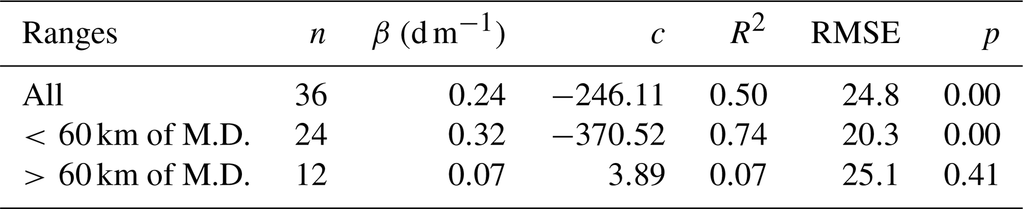
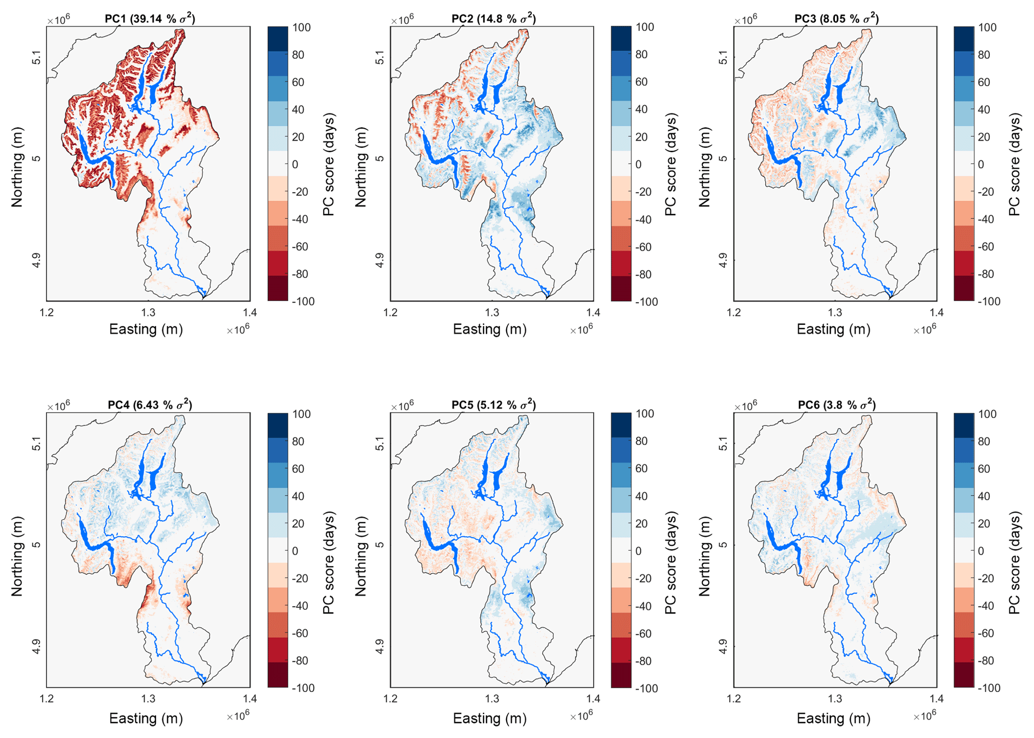
Figure 11The first six spatial principal components of the SCD anomaly.
4.3.4 Spatio-temporal variability in SCD across mountain ranges
A semi-distributed analysis of the SCD by mountain range provides further insight into spatial variability of SCD within the catchment. Since the mean elevation varies for each mountain range, the influence of elevation on SCD could be assessed. The mean annual SCD of individual mountain ranges is shown in Fig. 13, which demonstrates that average SCD is a function of elevation, as well as proximity to the Main Divide. For ranges within 60 km of the Main Divide, a significant positive correlation exists between mean range elevation and SCD, with the modelled relationship predicting an elevation of 2298 m for perennial snow cover. Beyond distances of 60 km from the Main Divide, however, the relationship weakens substantially and loses significance (Table 3). The deterioration of the relationship between elevation and SCD for ranges distant from the Main Divide suggests that the influence of temperature on SCD is substantially reduced in these cases.
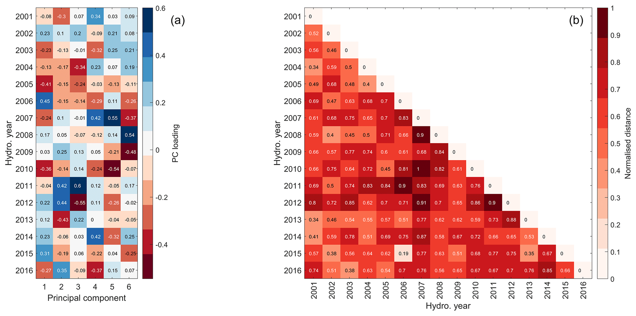
Figure 12(a) Loadings for the first six principal components of the SCD anomaly (77 % of total variance) for each hydrological year (which corresponds with the winter of the preceding calendar year). (b) Normalised distance between PC loadings.
For 4 out of the 16 winters analysed (25 %), the sign of the anomaly was out of phase across the catchment. For the winters of 2000 and 2003, the SCD anomaly was positive in the west and negative in the east, while the winters of 2008 and 2010 were negative in the west and positive in the east. These similarities are consistent with these pairs of years being grouped together on the basis of PC loadings. The spatial gradients of the SCD anomaly observed for these years, from west to east, are consistent with the derived principal components. PC2 and PC3, in particular, characterised the east–west gradient in the SCD anomaly which typifies these “out-of-phase” years. Both of these principal components expressed an east–west contrast in SCD anomaly, with PC2 emphasising an inverted topographic dependency. The winter of 2001 loaded negatively on PC2, while the winter of 2003 loaded negatively on both PC2 and PC3. Conversely, the winters of 2008 and 2010 loaded positively on both PC2 and PC3, with 2010 being the only winter to load strongly on both of these PCs. The consistent signal between PC signatures and the range anomaly approach demonstrates that both the fully distributed and range-based semi-distributed approaches are consistent in detecting variability in spatial contrasts. It also highlights that snow cover conditions across the Clutha Catchment are often spatially out of phase, with first-order control by elevation being of diminished importance. This out-of-phase behaviour, and indeed the variability in magnitude anomaly even when the entire catchment is in phase, confirms that processes at the sub-catchment scale are important in controlling variability in seasonal snow processes, and that influence of and sensitivity to competing climatic forcings varies across the catchment.
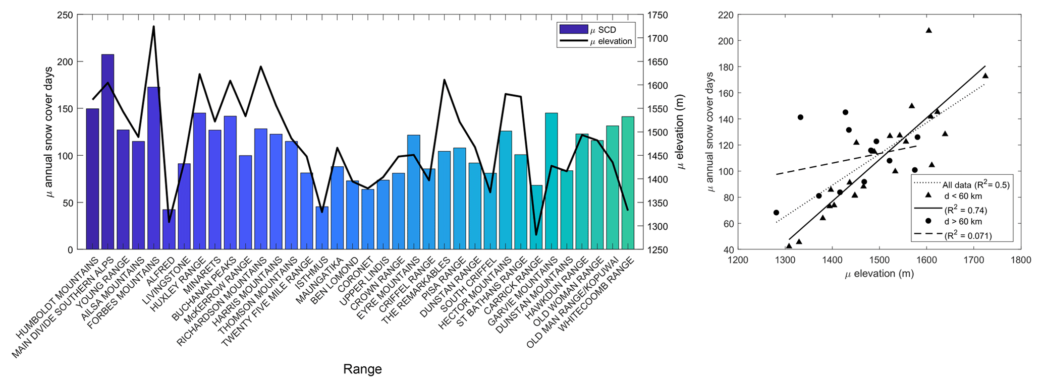
Figure 13Relationship between mean annual SCD and mean elevation of each mountain range. Ranges are sorted from left to right by their proximity to the Main Divide of the Southern Alps. The relationship between elevation and snow cover persistence was found to be much stronger in the western (within 60 km of the Main Divide) part of the catchment than in the east.
Table 4Parameters of regression between basin snow cover metrics and winter SOI and SAM values.
4.4 Climatic influences on SCD
4.4.1 Sensitivity of SCD to temperature and precipitation variability
Regression analysis between SCD, winter temperature and winter precipitation anomalies revealed a variable response across the catchment. Sensitivity to temperature and precipitation variability is expressed as days (d) per degree Celsius, or mm, respectively. Overall, relationships between temperature and precipitation anomalies and the SCD anomaly were found to be significant (p<0.05) across the catchment, yet both regressions featured high dispersion, with R2=0.19 for temperature and R2=0.11 for precipitation (Table S2). This dispersion was found to be due to contrasting climatic sensitivity across the catchment. For temperature, 50 % of ranges exhibited a statistically significant relationship between SCD and temperature anomaly. For all ranges, β was negative, with the greatest sensitivity of −53.6 d ∘C−1 occurring for the Ailsa Range. For precipitation, a significant relationship with SCD was found for 39 % of ranges. Values of β were always positive, with a maximum sensitivity of 0.11 d mm−1 occurring for the Eyre Mountains.
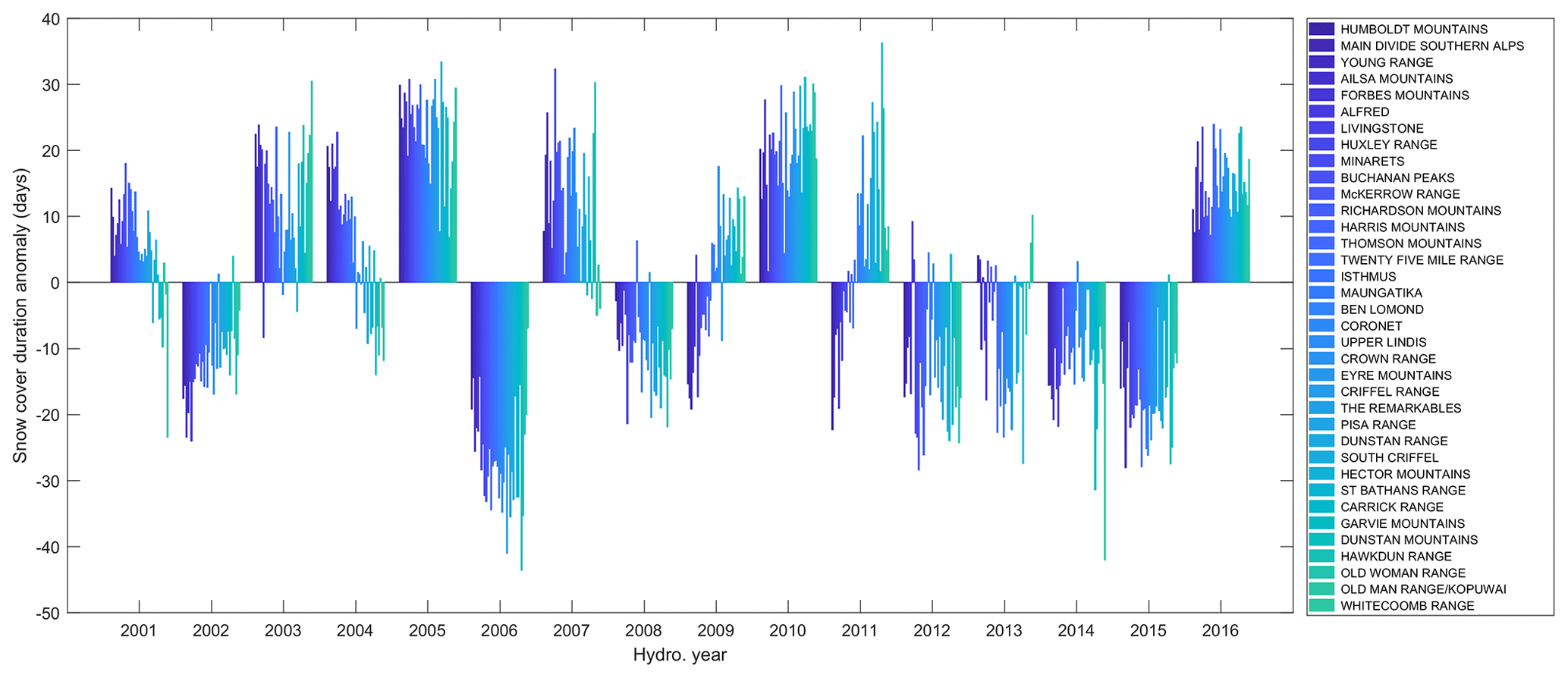
Figure 14SCD anomaly (in days) for geographic units of mountain ranges within the Clutha Catchment. Mountain ranges are sorted and symbolised by their proximity to the Main Divide of the Southern Alps, revealing spatial gradients in SCD anomaly across the catchment.
Sensitivity of the SCD anomaly to both temperature and precipitation anomalies was considered in terms of both elevation and proximity to the Main Divide and exhibited significant spatial trends (Figs. 15 and 16). Figure 15 reveals that distance to the Main Divide outperforms elevation at explaining variability in sensitivity to temperature. In the case of precipitation sensitivity, no relationship is evident with elevation, while a complex relationship with distance to the Main Divide is apparent.
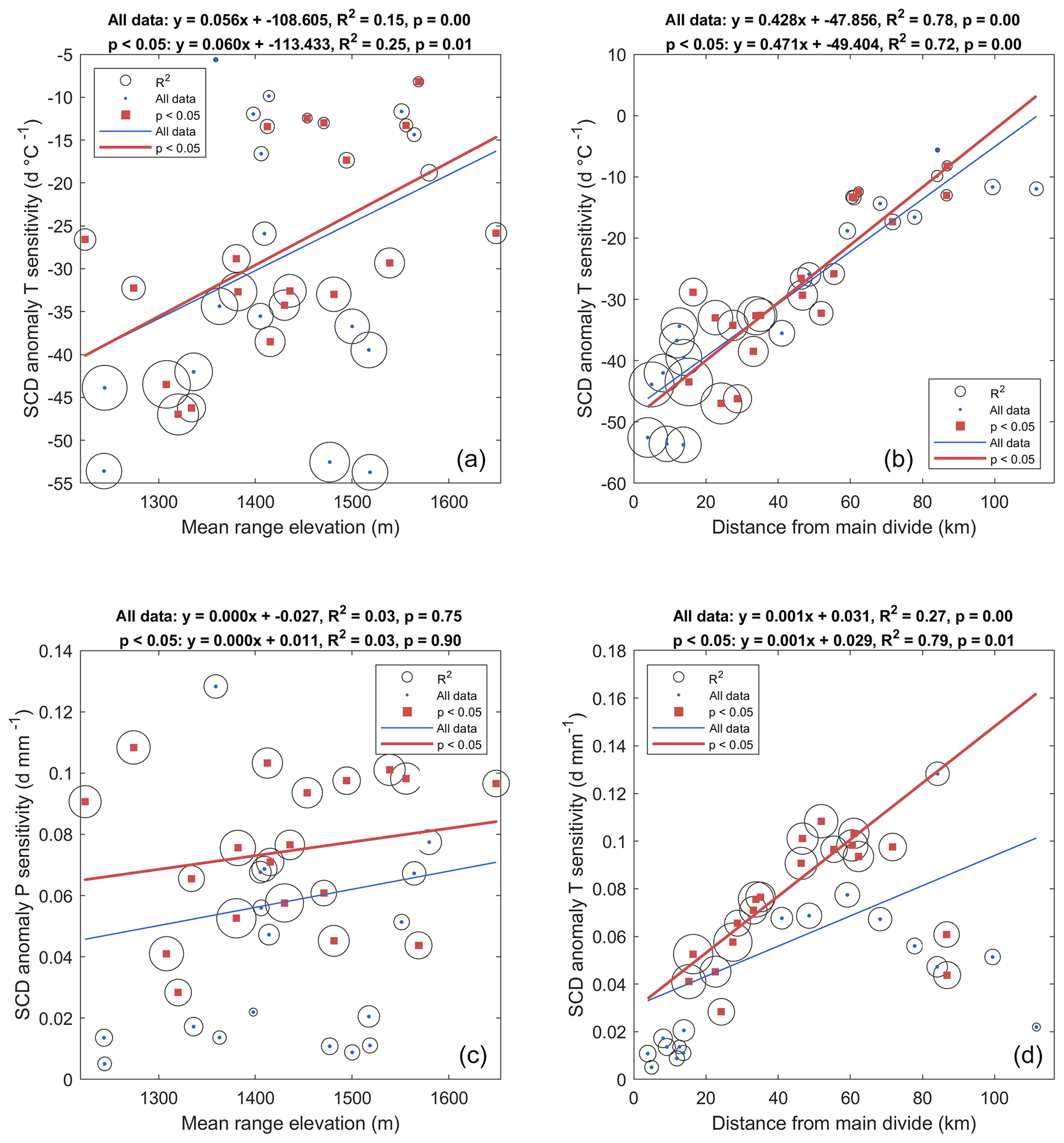
Figure 15Regressions between the sensitivity of SCD to temperature (a, b) and precipitation (c, d) in terms of mean elevation of each range for areas above the median winter snowline (a, c) and distance of each range from the Main Divide (b, d). In each case, regression is applied to all ranges, and to the subset for which p < 0.05 for range level sensitivity. Circular envelopes on data points are scaled by the R2 values associated with the regression for each mountain range.
Maximum temperature sensitivity occurred on and near the Main Divide, reducing at a rate of 0.43 d ∘C−1 km−1 eastward from the Main Divide, concurrently with decreasing R2 and increasing p values. The relationship between temperature anomaly and SCD anomaly becomes insignificant beyond distances of 55 km from the Main Divide. For precipitation, a more complex spatial trend emerged, whereby the relationship with SCD anomaly was weak and insignificant for ranges on and near the Main Divide, before becoming significant and strengthening with distance between 20 and 55 km, where the strongest significant relationship occurred. From this point, sensitivity to precipitation, as well as the strength of the relationship, decreased. The relationship between precipitation and SCD anomaly was insignificant at distances greater than 80 km from the Main Divide.
4.4.2 Influence of synoptic-scale variability
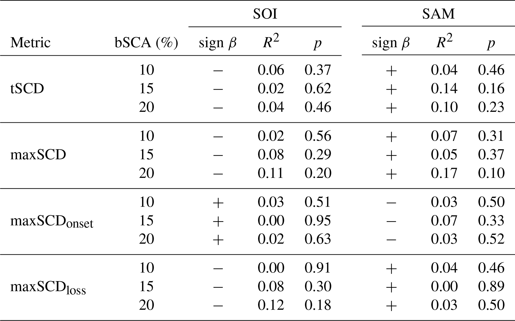
Both the SOI and SAM varied from year to year, yet notable events were limited to the strong La Niña of 2011. Relationships between basin snow cover metrics and the SOI and SAM were weak and insignificant (Table 4, Fig. S2). The lowest observed p value (0.16) was associated with a weak positive relationship between SAM and the total number of days of 15 % bSCA. Given the high inter-annual variability of bSCA relative to a lack of notable SOI or SAM events, any signal within these metrics is too weak to reveal any significant relationship with these indices over the 16-year period.
Table 5Parameters for significant (p≤0.05) linear multiple regression models between PC loadings and north-east (NE), east (E), south-east (SE) and south (S) trajectory frequency anomalies over varying time periods. Significant (p≤0.05) predictive variables are denoted by ∗.
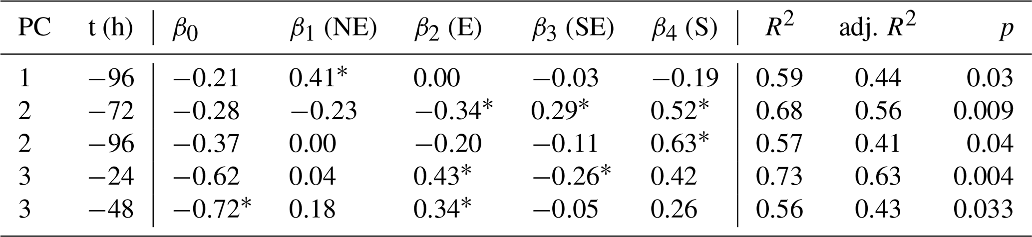
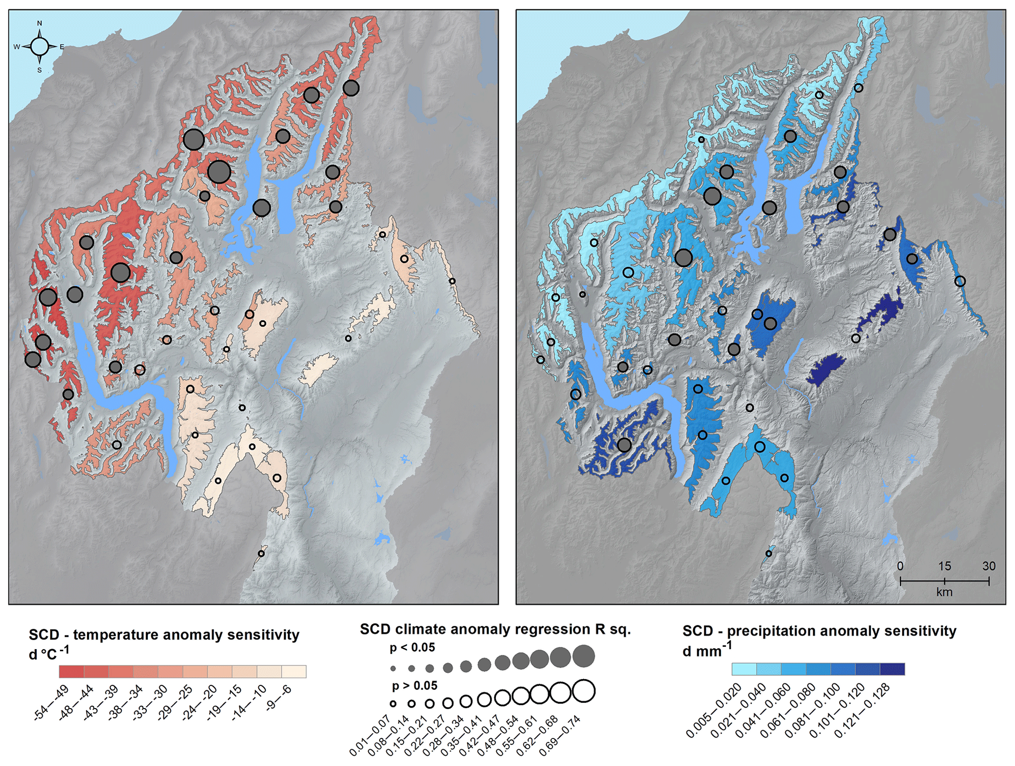
Figure 16Spatial variability in the regression parameters of slope and R2 between SCD anomaly and temperature and precipitation anomalies for each mountain range within the Clutha Catchment. Elevation and relief data from Columbus et al. (2011); lake outlines sourced from the LINZ Topographic Database.
Similarly, there was no significant correlation detected between the SAM and the yearly loadings of principal components one to six. In the case of SOI, PC2 displayed a relatively weak positive relationship (p=0.06, R2=0.23) and PC5 a relatively weak negative relationship (p=0.07, R2=0.21). These results suggest that the positive expression of PC2 is likely to be favoured during periods of positive SOI phase (La Niña), and PC5 during periods of negative SOI phase (El Niño). Furthermore, the enhanced signal provided by the PCs in this case highlights the benefit of utilising PCA to leverage the spatial structure of the SCA time series.
Comparison between the most anomalous years in terms of airflow, as characterised by HYSPLIT, and principal component loadings revealed associations between airflow and SCD anomaly. This is demonstrated for HY 2011, which was characterised by a substantial positive anomaly in easterly airflow. This corresponded with large positive loadings for both PC2 and PC3, the only year for which this occurred. Multiple linear regression between loadings for PCs one to six and the relative frequency of air mass origins for 24–96 h periods revealed strong correlations in only a few cases (Table 5). The associations that emerge from this analysis suggest that PC3 is associated with positive anomalies in easterly airflow, negative anomalies in south-easterly airflow over periods of 24 h and positive anomalies in easterly airflow over 48 h. PC2 was most strongly associated with negative easterly and positive south-easterly and southerly airflow anomalies over 72 h periods, as well as positive southerly airflow anomalies over 96 h periods. PC1 was most strongly associated with positive anomalies in north-easterly airflow over 96 h periods.
Comparison between the most anomalous years in terms of airflow, as characterised by HYSPLIT, and principal component loadings revealed associations between airflow and the SCD anomaly. This is demonstrated for HY 2011, which was characterised by a substantial positive anomaly in easterly airflow. This corresponded with large positive loadings for both PC2 and PC3, the only year for which this occurred. Multiple linear regression between loadings for PCs one to six and relative frequency of air mass origins for 24–96 h periods revealed strong correlations in only a few cases (Table 5). The associations that emerge from this analysis suggest that PC3 is associated with positive anomalies in easterly airflow, negative anomalies in south-easterly airflow over periods of 24 h and positive anomalies in easterly airflow over 48 h. PC2 was most strongly associated with negative easterly and positive south-easterly and southerly airflow anomalies over 72 h periods, as well as positive southerly airflow anomalies over 96 h periods. PC1 was most strongly associated with positive anomalies in north-easterly airflow over 96 h periods.
5.1 Spatial trends in seasonal snow cover
First-order topographic controls were found to exert substantial influence over mean SCD. Overall, SCD is strongly linked to elevation and aspect. This relationship was strongest on and near the Main Divide, with the relationship between elevation and mean SCD breaking down in the fault block ranges located > 60 km east of the Main Divide, as shown in Fig. 13. Maximum SCD and the only regions of perennial snow cover coincide with those areas of highest terrain and maximum mean annual precipitation along and near the Main Divide of the Southern Alps.

Figure 17(a) Mean monthly atmospheric pressure (mean sea level) plotted for five climate stations within the Clutha Catchment. Record lengths vary from 8 (dashed lines) to 16 years (solid lines). (b) Anomalies in winter mean air temperature for low elevation stations in the Clutha Catchment. Anomalies for each station were calculated with respect to the mean of the station record. Data from the NIWA National Climate Database (CliFlo) (NIWA, 2018).
The deterioration in the relationship between mean SCD and elevation for ranges south-east of the Main Divide suggests that the role of temperature as a primary control on SCD weakens for this region. Although not specifically studied here, a reduced frequency of cloud cover in the leeward rain shadow of the Main Divide may increase the relative importance of shortwave radiation in controlling ablation processes on eastern ranges. While the western ranges are alpine in nature, with high relief, the eastern ranges are characterised by high plateaus, with maximum elevations of 1400–1800 m. These plateaus are dissected by shallow basins and steep-sided gullies, the floors of which are typically above the winter snowline. This morphology, combined with exposure to persistent winds, is conducive to preferential accumulation during redistribution events, promoting the development of deep snowpacks (Redpath et al., 2018) which may persist much longer into spring than would otherwise be expected. The relative importance of competing climatic influences on SCD is discussed further in the following sections.
Overall, variability relative to the mean snow cover climatology is found to be high. The coefficient of variation is negatively correlated to elevation, and greatest for pixels with aspect N-NE, consistent with the anticipated influence of topographic variables as first-order controls. The fact that much of the catchment exhibits CVSCD > 100 % reflects the basin hypsometry. Most of the catchment remains below the mean winter snowline elevation, yet is still subject to occasional, often short-lived, snowfall events. A relatively large area of the catchment lies at elevations between 1000 and 1500 m and has CVSCD > 0.5, representing a large marginal snow season zone, where snow cover is often transient. Much of this area is in the eastern part of the catchment (e.g. the Hawkdun Range), where substantial inter-annual variability in SCD is observed.
5.2 Temporal trends in seasonal snow cover
Since 1909, annual mean temperature in New Zealand has increased at a rate of 0.91 ∘C per century, although this rate is reduced for the southern South Island (0.58 ∘C per century at Dunedin) (Mullan et al., 2010), and climate change is expected to result in a reduction in both the duration of snow cover, and peak snow depth in the South Island of New Zealand (Hendrikx et al., 2012). The 16-year time series presented here, however, remains largely dominated by inter-annual variability, concealing any temporal trend that may exist in SCD or SLE. This indicates that for the 2000–2016 period, short-term variability in seasonal snow exceeds any longer-term signal driven by climate change, which contrasts a tendency toward warmer than average air temperatures within the Clutha Catchment (Fig. 17). While this daily observational record of snow presence remains short, it is consistent with earlier findings of Fitzharris and Garr (1995), whose snow storage index reconstructed by temperature-index models (in turn driven by sparse observations) for the major hydro-electric catchments of the South Island showed significant inter-annual variability, but no long-term trend over the period 1931–1993. Subsequently, the Clutha Catchment exhibits contrasting behaviour to many other regions globally, where reductions in seasonal snow and shifts in the timing of seasonal snow processes have been observed (e.g. McCabe and Clark, 2005; Lundquist et al., 2009; Estilow et al., 2015; Klein et al., 2016; Borman et al., 2018). This includes other regions in the Southern Hemisphere, where in the Snowy Mountains of Australia a significant reduction in snow season length has been detected from MODIS data over the period 2000–2010 (Bormann et al., 2012). Similarly, the South American Andes have undergone a spatially variable but significant reduction in snow season length of 2–5 d yr−1 between latitudes 29 and 36∘ S over the period 2000–2016 (Saavedra et al., 2017). Despite the large observed inter-annual variability, the most extreme years in the current record can provide insight into the potential impact of future warming. The greatest reduction in snow cover across most metrics considered here occurred for HY 2006, during which SCD depletion was spatially consistent across the catchment (strong positive loading on PC1). This year represents an anomalously warm winter within the catchment, where temperatures at Queenstown Airport were 1 ∘C warmer than the 2000–2016 average (NIWA, 2018), and was characterised by high temperatures and higher than normal sunshine hours across much of the lower South Island (Salinger and Burgess, 2005). Relative to the 1986–2005 period, winter warming of 0.7–1.2 ∘C is projected for the Otago Region for the period 2031–2050 (Mullan et al., 2016). Considering the impact of temperature alone, the probability of poor snow seasons such as that seen for HY 2006 is likely to increase.
5.3 Spatio-temporal variability in seasonal snow cover
The relatively large number of principal components required to explain the main share of observed variability and the high dissimilarity between years in terms of PC loadings confirm the high degree of spatio-temporal variability within the time series. PC1 represents the largest share of variance in SCD and is explained by elevation, with most variance occurring in the areas where seasonal snow mostly occurs and persists. PC2, however, reveals an annular pattern, whereby negative deviation occurs at high elevations, and positive deviation at low elevations. The maximum positive loading on PC2 occurred for HY 2012, which also coincided with the latest observed onset date for 10 % bSCA and an extended period of anomalously high SLE. This characteristic in SCA and SLE was eventually reversed, with the latter part of the winter featuring a sustained period of suppressed SLE and higher than average SCA. Ultimately, this resulted in a longer than usual SCD at low elevations, despite the reduced SCD at high elevations due to an absence of autumn and early winter snow. The two most similar hydrological years in terms of PC loadings were 2006 and 2015. Both featured strong positive loadings on PC1 and negative loadings on most of the remaining PCs except for PC5. This resulted in strongly negative SCD anomalies for both years making them the two lowest ranked observed snow seasons across the catchment across the majority of metrics. Strong negative SCD anomalies affected all mountain ranges for these years.
Four years exhibited strong spatial gradients across the catchment, with an east–west gradient in positive to negative SCD anomalies for 2001 and 2003 and a west–east gradient for 2009 and 2011. While each pair shared similar loadings for some PCs, their overall pair-wise signature difference was still relatively high. This observation highlights that even for years that appear to be similar in terms of spatial variability in the SCD anomaly, the propagation of spatial variability across the catchment remains complex and highly variable from year to year. Notably, the occurrence of an east–west gradient in SCD anomaly and positive loadings on PCs 2, 3, 4 and 5 indicate that the typical climatic gradient (west–east) across the catchment can be modulated, or even reversed, in terms of SCD. The spatial structure evident across the catchment within PCs 2–6 also indicates that in terms of seasonal snow the Clutha Catchment departs substantially from behaving as a single climatic unit.
5.4 Climatic influences on observed snow cover variability
5.4.1 Influence of winter blocking highs
A persistent feature throughout the 16-year time series was the observed mid-winter decrease in bSCA, which on average occurs during July, before SCA peaks again in August. This feature of the snow cover climatology aligns with a winter positive air pressure anomaly, which peaks in July (Fig. 17). The occurrence of winter anticyclones is a common feature in the New Zealand region, and these may commonly become persistent and lead to strong blocking (Sinclair, 1996). Under such conditions, the frequency of precipitation events (i.e. snowfall), particularly those delivered by the passage of fronts, will be reduced, while at the same time, solar irradiance at the surface will be high under clear sky conditions. Together, these factors will reduce accumulation and enhance ablation, allowing a depletion in SCA before unsettled conditions in late winter and early spring promote renewed accumulation and bSCA increases again ahead of spring melt.
5.4.2 Temperature and precipitation sensitivity and associated spatial variability
In a global context, Hammond et al. (2018) found southern New Zealand to be mixed in terms of the relative importance of temperature and precipitation variability in influencing snow persistence. Here, a thorough spatial analysis allows the relative importance of temperature and precipitation to be further scrutinised in more detail. Temperature was found to have a more significant influence on SCD anomaly than precipitation, although sensitivity to both factors was spatially variable. Sensitivity to both temperature and precipitation was more strongly associated with proximity to the Main Divide than elevation. The sensitivity of the SCD anomaly to temperature was greatest on and near to the Main Divide, where sensitivities as high as −53 d ∘C−1 were observed, accompanied by significant R2 values of 0.39–0.74. Sensitivity decreased to the east, with the weakest relationship of −6 d ∘C−1 (R2=0.01, p=0.78) observed for the Dunstan Mountains. Enhanced sensitivity to temperature on and near the Main Divide reflects the influence of orographic processes, with the rain–snow temperature threshold and associated albedo feedback playing important roles in controlling accumulation and ablation in this cloudy, high-precipitation environment. Conversely, increased incident solar irradiance through the central part of the catchment (Macara, 2015) and an increased proportion of precipitation delivered via cold fronts may act to reduce the importance of air temperature in controlling snow accumulation and ablation. For the Brewster Glacier, located west of the Main Divide and just outside the Clutha Catchment, Cullen and Conway (2015) reported that net radiation dominated melt at annual timescales, but the role of cloud cover in enhancing sensitivity to air temperature at Brewster Glacier has also been recognised (Conway and Cullen, 2016). The Pisa Range, near the geographic centre of the catchment, has a temperature sensitivity of −13.28 d ∘C−1 (R2=0.06 , p=0.38), which is broadly consistent with the findings of Sims and Orwin (2011) where net radiation provided 40 % of melt energy, compared to 34 % from sensible heat fluxes. Conversely, further north in Canterbury's Craigieburn Range, which is also east of the Main Divide, Prowse and Owens (1982) found that sensible heat dominated melt energetics, which suggests that spatial gradients in climatic sensitivity are not uniform across the South Island. Further complicating the relative importance of turbulent and radiative fluxes in controlling ablation processes is the role of wind entrainment. As discussed previously, wind re-distribution of snow is likely to result in concentration of snow as promoted by topography and can promote ablation of the snow pack by sublimation under favourable conditions (Pomeroy and Gray, 1990; Pomeroy and Essery, 1999; Wang and Jia, 2018). Preferentially accumulated snow will generally increase in density and depth, further increasing the energy required to ablate the snow pack. The increased rate at which mean SCD lengthens with elevation on southerly aspects compared to northerly aspects further supports this interpretation.
Spatial variability in the sensitivity of seasonal snow to climatic parameters has been detected elsewhere. Howat and Tulaczyk (2005), for example, detected spatial variability in the sensitivity of maximum spring SWE to climate forcings in the predominantly precipitation-sensitive Sierra Nevada of California. While a portion of observed sensitivity was attributed to elevation, an unexplained latitudinal dependence was attributed to contrasting regional atmospheric circulation patterns. As pointed out by Howat and Tulaczyk (2005), observations of spatial variability in temperature sensitivity may lead to over-predictions of reduced snow cover by models that lack sufficient spatial scale or parameterisation. As well as providing a reference dataset for model calibration and validation, these findings can provide guidance for efforts to model seasonal snow processes at the catchment to national scale in the New Zealand context. Understanding the relative importance of precipitation and temperature and their influence on seasonal snow is central to evaluating and refining the performance of degree-day models. It is clear, for example, that such models may perform adequately at recreating melt on and near the Main Divide, their performance will likely deteriorate for ranges further east, where the relative importance of variability in energy balance and wind-driven redistribution of snow is increased. Hock (2003) emphasised that while degree-day models work well for modelling melt at catchment scales over long time periods, reliability is reduced as temporal resolution increases and where spatial variability in melt rates exist. Similarly, Clark et al. (2009) suggested that basin-specific parameterisations are required to improve the simulation of seasonal snow across the South Island, and these results can provide guidance to this end within the Clutha Catchment, as well as providing a framework for the assessment of snow cover sensitivity to climatic forcings that could be scaled up across the South Island.
There is a need to better understand the relative importance of temperature and precipitation sensitivity, in particular to better capture the potential for gains in snow accumulation through increased precipitation to offset losses driven by increased temperature. Furthermore, the current study indicates that considering just temperature and precipitation leaves a large component of SCD variability unexplained, emphasising the need to improve understanding and parameterisation of individual components of the energy balance and redistribution of snow by wind. Degree-day models may be enhanced relatively simply through the inclusion of radiation and albedo factors. Gao et al. (2017) demonstrate the increased transferability introduced to hydrological models of snow- and glacier-dominated catchments when improved representations of topographic heterogeneity are included. Capturing the effects of wind on snow redistribution, however, remains a substantial challenge, further compounded by a scarcity of data in alpine environments such as New Zealand (Hendrikx and Harper, 2013) and the need to characterise terrain at sufficient resolution to resolve wind-driven processes at relevant scales (e.g. Marsh et al., 2018; Mott et al., 2018).
5.4.3 Atmospheric circulation
The association between HYSPLIT trajectory anomalies and characteristic spatial variability in SCD, as expressed by PC loadings, provides new insight into the role of anomalous synoptic-scale circulation on snow cover variability. For HY 2011 in particular, relatively high positive loadings were identified for PC2 and PC3, which are both associated with positive anomalies in SCD in the eastern part of the catchment (particularly the Manuherikia basin) and, in the case of PC2, relatively strong positive anomalies in SCD at low elevations across the catchment. HYSPLIT trajectory anomalies for this period revealed a substantial increase in the frequency of airflow originating to the east of New Zealand. This scenario of anomalous easterly airflow represents a reversal of the typical zonal flow affecting the South Island of New Zealand, which is dominated by westerly flow (Sturman and Tapper, 2006; Macara, 2015) whereby the eastern part of the catchment lies in the rain shadow of the Southern Alps. Under easterly flow conditions, topographic barriers between the Pacific Ocean and the ranges of the eastern part of the catchment are substantially reduced. The 2011 hydrological year also featured the highest observed mean winter SOI value (i.e. the strongest observed La Niña event).
Overall, the climatic indices of SOI and SAM did not provide strong explanations for spatio-temporal variability of snow cover within the Clutha Catchment. A notable exception to this was HY 2012. This year had the largest positive loading on PC2, corresponding to an annular spatial pattern in SCD anomaly with positive anomalies at low elevations and negative anomalies at high elevations. Climatically, this HY was characterised by strong positive SOI values (i.e. La Niña conditions) from February 2011, which weakened somewhat by June before strengthening again through to December (Renwick, 2012). At the same time, the SAM switched from positive in May to near neutral in June, before remaining strongly negative from July to September. Subsequently, this snow season was substantially shortened at high elevations, due to a reduction in accumulation early in winter. Conversely, the persistently negative SAM through late winter was accompanied by a period of regular low-level snowfall that extended SCD at low elevations. The lack of strong relationships with SOI and SAM differs somewhat from the observations of Hammond et al. (2018), who detected a correlation between the Oceanic Niño Index and snow persistence across a substantial proportion of the lower South Island. Varying results here may be a result of the different spatial scales of analysis.
The most reduced SCD across the catchment occurred for HYs 2006 and 2015, which were also the most similar in terms of PC loadings. In particular, PC1 was associated with positive anomalies in airflow originating north-east of New Zealand. While positive SOI values (e.g. La Niña conditions) are associated with anomalous north-easterly flow for New Zealand (Sturman and Tapper, 2006), these years were associated with both slightly positive (HY 2006) and negative (HY 2015) winter mean SOI values, while both have positive anomalies in the frequency of north-easterly airflow. This analysis highlights that, despite the complex interacting processes governing seasonal snow cover in New Zealand, large-scale climatic perturbations can be linked to the spatio-temporal distribution of seasonal snow cover, beyond controls imposed by regional topography. An expected future strengthening of winter westerlies for the lower South Island (Mullan et al., 2016) would decrease the likelihood of extended SCD in the eastern part of the Clutha Catchment, through a corresponding reduction in winter easterly flow, which is important for delivering precipitation to the Manuherikia Basin.
5.5 Limitations of scale
The large number of principal components required to explain the observed variability suggest that some of the spatial variability affecting seasonal snow within the Clutha Catchment occurs beyond the detection limits of MODIS. While an inability to resolve fine-scale processes limits insights into the full range of processes controlling seasonal snow within the catchment, spatial variability in sensitivity of SCD to changes in temperature and precipitation has been demonstrated at a sub-catchment scale. Furthermore, the observed degradation of the relationship between SCD and elevation away from the Main Divide (Fig. 13) suggests the processes occurring at scales that are difficult to detect with MODIS gain significance in controlling SCD. These processes include re-distribution of snow by wind and the associated influence of micro-terrain, which may complicate the interpretation of pixel-level fSCA. This is likely to be especially relevant to hydrological modelling and demands further attention on fine-scale spatial variability in seasonal snow.
This study has produced a 16-year time series of daily snow-covered area from MODIS imagery for the Clutha Catchment, New Zealand, providing an important supplement to sparse seasonal snow observations in the Southern Hemisphere. From the daily SCA time series, a number of metrics have been derived to characterise the spatio-temporal variability of seasonal snow cover for this region. A consistent reduction in mid-winter SCA demonstrates the influence of persistent synoptic-scale features, such as blocking highs. Overall, the inter-annual variability is high, concealing any trend that may exist over the study period. Despite the lack of a temporal trend in this record, extreme years provide insight into conditions that may become more frequent under future climate change scenarios.
Characterisation of spatial modes of variability via spatialised rPCA reinforces the highly dynamic nature of seasonal snow cover within the catchment, with minimal similarity in spatial patterns between years. Nonetheless, this analysis proved capable of identifying the two most similar years for which spatial patterns of SCD were linked to anomalous north-easterly airflow. The ability to identify such associations highlights the strength of the approach taken to rPCA, which retained both the spatial and temporal signals of SCD variability. Spatial variability in snow cover across the catchment is also high, with the SCD anomaly being out of phase for some years, indicating that the Clutha Catchment departs markedly from a single climatic unit in terms of seasonal snow.
Spatial variability in the sensitivity of SCD to temperature and precipitation variability at sub-catchment scale has also been demonstrated. Temperature was found to be an important control of SCD variability on and near the Main Divide. Precipitation was important in the east of the Main Divide, but insignificant for ranges further east. On their own, these two variables leave a large proportion of SCD variability unexplained. While providing guidance for efforts to improve parameterisations of snow models in New Zealand, these findings also highlight the likely importance of other components of the energy balance and the redistribution of snow by wind in influencing seasonal snow processes, and subsequent shortcomings in traditional degree-day approaches to modelling seasonal snow in this region. In demonstrating the utility of rPCA for examining spatio-temporal variability in SCD at regional scales, this work provides a framework for the ongoing monitoring of seasonal snow cover, improves the context for understanding the snow hydrology of the Clutha Catchment, and can contribute to efforts to improve the modelling of seasonal snow throughout New Zealand and elsewhere, particularly where in situ records are sparse.
The MODImLab software is available on request from Pascal Sirguey. The MODIS data used in this research were acquired from the Level-1 and Atmosphere Archive & Distribution System (LAADS) Distributed Active Archive Center (DAAC), located in the Goddard Space Flight Center in Greenbelt, Maryland, USA (https://doi.org/10.5067/MODIS/MOD03.006, MODAPS, 2012a; https://doi.org/10.5067/MODIS/MOD021KM.006, MODAPS, 2012b).
The supplement related to this article is available online at: https://doi.org/10.5194/hess-23-3189-2019-supplement.
TANR, PS and NJC designed the study. TANR and PS processed and analysed the data. PS developed and maintains the MODImLab software. TANR prepared the paper with contributions from all authors.
The authors declare that they have no conflict of interest.
We are grateful to Andreas Jobst for providing gridded temperature and precipitation data for the Clutha Catchment. Sean Fitzsimons provided helpful feedback on the draft manuscript. Elevation and relief data in Figs. 1, 3, 5, and 16 were sourced from the NZSoSDEM v1.0, which is available under CC BY-SA 2.0 at https://koordinates.com/publisher/university-of-otago-national-school-of-surveying/ (last access: 15 October 2017). Lake outlines and geographic names included in Figs. 1, 3, 4, 5, and 16 were sourced from the NZ Topographic Database, available under CC-BY 4.0 (Crown Copyright Reserved) from https://data.linz.govt.nz (last access: 3 March 2017). Stream network and catchment boundaries were sourced from the MfE River Environments Classification New Zealand, available under CC-BY 3.0 from https://data.mfe.govt.nz (last access: 24 May 2017). The authors thank the reviewers and editor whose thorough and thoughtful comments improved the paper.
This research has been supported by a University of Otago Doctoral Scholarship.
This paper was edited by Markus Hrachowitz and reviewed by two anonymous referees.
Andersen, T.: Operational snow mapping by Satellites, Hydrological Aspects of Alpine and High Mountain Areas (Proceedings of the Exeter Symposium), IAHS Publ. no. 138, 1982. a
Baba, K. and Renwick, J.: Aspects of intraseasonal variability of Antarctic sea ice in austral winter related to ENSO and SAM events, J. Glaciol., 63, 1–9, https://doi.org/10.1017/jog.2017.49, 2017. a
Barnes, W. L., Pagano, T. S., and Salomonson, V. V.: Prelaunch characteristics of the Moderate Resolution Imaging Spectroradiometer (MODIS) on EOS-AM1, IEEE T. Geosci. Remote, 36, 1088–1100, https://doi.org/10.1109/36.700993, 1998. a
Barnett, T. P., Adam, J. C., and Lettenmaier, D. P.: Potential impacts of a warming climate on water availability in snow-dominated regions, Nature, 438, 303–309, https://doi.org/10.1038/nature04141, 2005. a
Barringer, J. R. F.: A Variable Lapse Rate Snowline Model for the Remarkables, Central Otago, New Zealand, J. Hydrol., 28, 32–46, 1989. a
Bessho, K., Date, K., Hayashi, M., Ikeda, A., Imai, T., Inoue, H., Kumagai, Y., Miyakawa, T., Murata, H., Ohno, T., Okuyama, A., Oyama, R., Sasaki, Y., Shimazu, Y., Shimoji, K., Sumida, Y., Suzuki, M., Taniguchi, H., Tsuchiyama, H., Uesawa, D., Yokota, H., and Yoshida, R.: An Introduction to Himawari-8/9 – Japan's New-Generation Geostationary Meteorological Satellites, J. Meteorol. Soc. Jpn., 94, 151–183, https://doi.org/10.2151/jmsj.2016-009, 2016. a
Borman, K. J., Brown, R. D., Derksen, C., and Painter, T. H.: Estimating snow-cover trends from space, Nat. Clim. Change, 8, 924–936, https://doi.org/10.1038/s41558-018-0318-3, 2018. a, b, c
Bormann, K. J., McCabe, M. F., and Evans, J. P.: Satellite based observations for seasonal snow cover detection and characterisation in Australia, Remote Sens. Environ., 123, 57–71, https://doi.org/10.1016/j.rse.2012.03.003, 2012. a, b
Brown, C. E.: Applied multivariate statistics in geohydrology and related sciences, Springer, Berlin, New York, 1998. a
Brunk, T. and Sirguey, P.: An updated map of New Zealand's permanent snow and ice cover, Tech. rep., National School of Surveying, University of Otago, 2018. a, b
Campbell, A. J., Hulbe, C. L., and Choon-Ki, L. E.: The shape of change: An EOF approach to identifying sources of transient thickness change in an ice shelf, Ann. Glaciol., 58, 21–27, https://doi.org/10.1017/aog.2017.16, 2017. a
Clark, M., Hreinsson, E. Ö., Martinez, G., Tait, A., Slater, A., Hendrikx, J., Owens, I., Gupta, H., Schmidt, J., and Woods, R.: Simulations of seasonal snow for the South Island , New Zealand, J. Hydrol., 48, 41–58, 2009. a, b
Columbus, J., Sirguey, P., and Tenzer, R.: A free fully assessed 15 metre digital elevation model for New Zealand, Survey Quarterly, 66, 16–19, 2011. a, b, c, d, e, f
Conway, J. P. and Cullen, N. J.: Cloud effects on surface energy and mass balance in the ablation area of Brewster Glacier, New Zealand, The Cryosphere, 10, 313–328, https://doi.org/10.5194/tc-10-313-2016, 2016. a
Cullen, N. J. and Conway, J. P.: A 22 month record of surface meteorology and energy balance from the ablation zone of Brewster Glacier, New Zealand, J. Glaciol., 61, 931946, https://doi.org/10.3189/2015JoG15J004, 2015. a
Dean, S. M. and Stott, P. A.: The Effect of Local Circulation Variability on the Detection and Attribution of New Zealand Temperature Trends, J. Climate, 22, 6217–6229, https://doi.org/10.1175/2009JCLI2715.1, 2009. a
Demšar, U., Harris, P., Brunsdon, C., Fotheringham, A. S., and McLoone, S.: Principal Component Analysis on Spatial Data: An Overview, Ann. Assoc. Am. Geogr., 103, 106–128, https://doi.org/10.1080/00045608.2012.689236, 2012. a, b, c
Dozier, J.: Spectral signature of alpine snow cover from the Landsat Thematic Mapper, Remote Sens. Environ., 22, 9–22, 1989. a
Dozier, J., Painter, T. H., Rittger, K., and Frew, J. E.: Time-space continuity of daily maps of fractional snow cover and albedo from MODIS, Adv. Water Resour., 31, 1515–1526, https://doi.org/10.1016/j.advwatres.2008.08.011, 2008. a, b, c
Dozier, J., Green, R. O., Nolin, A. W., and Painter, T. H.: Remote Sens. Environ. Interpretation of snow properties from imaging spectrometry, Remote Sens. Environ., 113, S25–S37, https://doi.org/10.1016/j.rse.2007.07.029, 2009. a
Drolon, V., Maisongrande, P., Berthier, E., Swinnen, E., and Huss, M.: Monitoring of seasonal glacier mass balance over the European Alps using low-resolution optical satellite images, J. Glaciol., 62, 1–16, https://doi.org/10.1017/jog.2016.78, 2016. a
Dunteman, G. H.: Principal components analysis, Quantitative applications in the social sciences, SAGE Publications, Inc., Newbury Park, California, https://doi.org/10.4135/9781412985475, 1989. a
Estilow, T. W., Young, A. H., and Robinson, D. A.: A long-term Northern Hemisphere snow cover extent data record for climate studies and monitoring, Earth Syst. Sci. Data, 7, 137–142, https://doi.org/10.5194/essd-7-137-2015, 2015. a, b, c, d
Fitzharris, B., Lawson, W., and Owens, I.: Research on glaciers and snow in New Zealand, Prog. Phys. Geog., 23, 469–500, https://doi.org/10.1177/030913339902300402, 1999. a
Fitzharris, B. B. and Garr, G. E.: Simulation of past variability in seasonal snow in the Southern Alps, New Zealand, Ann. Glaciol., 21, 377–382, 1995. a, b, c
Fitzharris, B. B. and Grimmond, C. S. B.: Assessing snow storage and melt in a New Zealand mountain Environment, Hydrological Aspects of Alpine and High Mountain Areas (Proceedings of the Exeter Symposium), IAHS Publ. no. 138., 1982. a
Fitzharris, B. B., Stewart, D., and Harrison, W.: Contribution of snowmelt to the October 1978 flood of the Pomohaka and Fraser Rivers, Otago, J. Hydrol., 19, 84–93, 1980. a
Fitzharris, B. B., Clare, G. R., and Renwick, J.: Teleconnections between Andean and New Zealand glaciers, Global Planet. Change, 59, 159–174, https://doi.org/10.1016/j.gloplacha.2006.11.022, 2007. a, b
Frey, R., Ackerman, S., Liu, Y., Strabala, K., Zhang, H., Key, J., and Wang, X.: Cloud Detection with MODIS. Part I: Improvements in the MODIS Cloud Mask for Collection 5, J. Atmos. Ocean. Tech., 25, 1057–1072, 2008. a
Gao, H., Ding, Y., Zhao, Q., Hrachowitz, M., and Savenije, H. H.: The importance of aspect for modelling the hydrological response in a glacier catchment in Central Asia, Hydrol. Process., 31, 2842–2859, https://doi.org/10.1002/hyp.11224, 2017. a
Gascoin, S., Hagolle, O., Huc, M., Jarlan, L., Dejoux, J.-F., Szczypta, C., Marti, R., and Sánchez, R.: A snow cover climatology for the Pyrenees from MODIS snow products, Hydrol. Earth Syst. Sci., 19, 2337–2351, https://doi.org/10.5194/hess-19-2337-2015, 2015. a, b, c
Hall, D. K., Riggs, G. A., Salomonson, V. V., Di Girolamo, N. E., and Bayr, K. J.: MODIS snow-cover products, Remote Sens. Environ., 83, 181–194, https://doi.org/10.1016/S0034-4257(02)00095-0, 2002. a, b, c
Hall, D. K., Crawford, C. J., Di Girolamo, N. E., Riggs, G. A., and Foster, J. L.: Detection of earlier snowmelt in the Wind River Range, Wyoming, using Landsat imagery, 1972–2013, Remote Sens. Environ., 162, 45–54, https://doi.org/10.1016/j.rse.2015.01.032, 2015. a
Hammond, J. C., Saavedra, F. A., and Kampf, S. K.: Global snow zone maps and trends in snow persistence 2001–2016, Int. J. Climatol., 38, 4369–4383, https://doi.org/10.1002/joc.5674, 2018. a, b, c
Haralick, R. M., Sternberg, S. R., and Zhuang, X.: Image Analysis Using Mathematical Morphology, IEEE T. Pattern Anal., 9, 532–550, https://doi.org/10.1109/TPAMI.1987.4767941, 1987. a
Hendrikx, J. and Harper, A.: Development of a national snow and ice monitoring network for New Zealand, J. Hydrol., 52, 83–95, 2013. a, b
Hendrikx, J. and Hreinsson, E. Ö.: The potential impact of climate change on seasonal snow in New Zealand: part II – industry vulnerability and future snowmaking potential, Theor. Appl. Climatol., 110, 619–630, https://doi.org/10.1007/s00704-012-0713-z, 2012. a
Hendrikx, J., Hreinsson, E. Ö., Clark, M. P., and Mullan, A. B.: The potential impact of climate change on seasonal snow in New Zealand: part – an analysis using 12 GCMs, Theor. Appl. Climatol., 110, 607–618, https://doi.org/10.1007/s00704-012-0711-1, 2012. a, b
Hinchey, L. W., Riddell, R. J., Engelbrecht, R. L., and Grant, R. D.: Report of Working Party on Central Otago Irrigation, report to Minister of Works and Development, 1981. a, b
Hock, R.: Temperature index melt modelling in mountain areas, J. Hydrol., 282, 104–115, 2003. a
Hopkins, D.: The sustainability of climate change adaptation strategies in New Zealand's ski industry: a range of stakeholder perceptions, J. Sustain. Tour., 22, 107–126, https://doi.org/10.1080/09669582.2013.804830, 2014. a, b
Hopkins, D.: The perceived risks of local climate change in Queenstown, New Zealand, Curr. Issues Tour., 18, 947–965, 2015. a, b
Howat, I. M. and Tulaczyk, S.: Climate sensitivity of spring snowpack in the Sierra Nevada, J. Geophys. Res., 110, F04021, https://doi.org/10.1029/2005JF000356, 2005. a, b
Jackson, J. E.: A User's Guide to Principal Components, John Wiley & Sons, New York, https://doi.org/10.1002/0471725331, 1991. a
Jobst, A. M.: The potential impacts of climate change on the hydro-climate of the Clutha/Mata-Au catchment, Phd, University of Otago, available at: https://otago.ourarchive.ac.nz/handle/10523/7334 (last access: 17 August 2018), 2017. a, b, c
Jobst, A. M., Kingston, D. G., Cullen, N. J., and Sirguey, P.: Combining thin-plate spline interpolation with a lapse rate model to produce daily air temperature estimates in a data-sparse alpine catchment, Int. J. Climatol., 37, 214–229, https://doi.org/10.1002/joc.4699, 2017. a, b
Jobst, A. M., Kingston, D. G., Cullen, N. J., and Schmid, J.: Intercomparison of different uncertainty sources in hydrological climate change projections for an alpine catchment (upper Clutha River, New Zealand), Hydrol. Earth Syst. Sci., 22, 3125–3142, https://doi.org/10.5194/hess-22-3125-2018, 2018. a, b, c
Kalnay, E., Kanamitsu, M., Kistler, R., Collins, W., Deaven, D., Gandin, L., Iredell, M., Saha, S., White, G., Woollen, J., Zhu, Y., Chelliah, M., Ebisuzaki, W., Higgins, W., Janowiak, J., Mo, K. C., Ropelewski, C., Wang, J., Leetmaa, A., Reynolds, R., Jenne, R., and Joseph, D.: The NCEP/NCAR 40-Year Reanalysis Project, B. Am. Meteorol. Soc., 77, 437–472, https://doi.org/10.1175/1520-0477(1996)077<0437:TNYRP>2.0.CO;2, 1996. a
Kerr, T.: The contribution of snowmelt to the rivers of the South Island, New Zealand, J. Hydrol., 52, 61–82, 2013. a, b, c
Kidston, J., Renwick, J. A., and McGregor, J.: Hemispheric-Scale Seasonality of the Southern Annular Mode and Impacts on the Climate of New Zealand, J. Climate, 22, 4759–4770, https://doi.org/10.1175/2009JCLI2640.1, 2009. a
Klein, G., Vitasse, Y., Rixen, C., Marty, C., and Rebetez, M.: Shorter snow cover duration since 1970 in the swiss alps due to earlier snowmelt more than to later snow onset, Climatic Change, 139, 637–649, https://doi.org/10.1007/s10584-016-1806-y, 2016. a, b
Krajčí, P., Holko, L., Perdigão, R. A. P., and Parajka, J.: Estimation of regional snowline elevation (RSLE) from MODIS images for seasonally snow covered mountain basins, J. Hydrol., 519, 1769–1778, https://doi.org/10.1016/j.jhydrol.2014.08.064, 2014. a, b, c
Lamont, G., Chinn, T., and Fitzharris, B.: Slopes of glacier ELAs in the Southern Alps of New Zealand in relation to atmospheric circulation patterns, Global Planet. Change, 22, 209–219, https://doi.org/10.1016/S0921-8181(99)00038-7, 1999. a
Landcare Research: LCDB v4.1 – Land Cover Database version 4.1, Mainland New Zealand, available at: https://lris.scinfo.org.nz/layer/48423-lcdb-v41-land-cover-database-version-41-mainland-new-zealand/ (last access: 16 August 2018), 2015. a
Lemmetyinen, J., Derksen, C., Rott, H., Macelloni, G., King, J., Schneebeli, M., Wiesmann, A., Leppänen, L., Kontu, A., and Pulliainen, J.: Retrieval of Effective Correlation Length and Snow Water Equivalent from Radar and Passive Microwave Measurements, Remote Sens., 10, 170, https://doi.org/10.3390/rs10020170, 2018. a
LINZ: NZ Geographic Names (Topo, 1:50k), available at: https://data.linz.govt.nz/layer/50280-nz-geographic-names-topo-150k/, last access: 3 March 2017. a
Lundquist, J. D., Dettinger, M. D., Stewart, I. T., and Cayan, D. R.: Variability and Trends in Spring Runoff in the Western United States, 63–76, University of Utah Press, 2009. a, b
Macara, G. R.: The Climate and Weather of Otago, NIWA Science and Technology Series 67, NIWA, 2015. a, b, c, d
Malenovský, Z., Rott, H., Cihlar, J., Schaepman, M. E., García-Santos, G., Fernandes, R., and Berger, M.: Sentinels for science: Potential of Sentinel-1, -2, and -3 missions for scientific observations of ocean, cryosphere, and land, Remote Sens. Environ., 120, 91–101, https://doi.org/10.1016/j.rse.2011.09.026, 2012. a
Mankin, J. S. and Diffenbaugh, N. S.: Influence of temperature and precipitation variability on near-term snow trends, Climate Dynamics, 45, 1099–1116, https://doi.org/10.1007/s00382-014-2357-4, 2015. a
Marsh, C. B., Spiteri, R. J., Pomeroy, J. W., and Wheater, H. S.: Multi-objective unstructured triangular mesh generation for use in hydrological and land surface models, Comput. Geosci., 119, 49–67, 2018. a
Marti, R., Gascoin, S., Berthier, E., de Pinel, M., Houet, T., and Laffly, D.: Mapping snow depth in open alpine terrain from stereo satellite imagery, The Cryosphere, 10, 1361–1380, https://doi.org/10.5194/tc-10-1361-2016, 2016. a
Masson, T., Dumont, M., Mura, M. D., Sirguey, P., Gascoin, S., Dedieu, J.-P., and Chanussot, J.: An Assessment of Existing Methodologies to Retrieve Snow Cover Fraction from MODIS Data, Remote Sens., 10, 619, https://doi.org/10.3390/rs10040619, 2018. a, b, c
McCabe, G. J. and Clark, M. P.: Trends and Variability in Snowmelt Runoff in the Western United States, J. Hydrometeorol., 6, 476–482, 2005. a, b
McKerchar, A. I., Pearson, C. P., and Fitzharris, B. B.: Dependency of summer lake inflows and precipitation on spring SOI, J. Hydrol., 205, 66–80, 1998. a, b
MODAPS (MODIS Characterization Support Team (MCST)/MODIS Adaptive Processing System): MODIS/Terra Geolocation Fields 5-Min L1A Swath 1 km, https://doi.org/10.5067/MODIS/MOD03.006 (last access: 31 October 2017), 2012a.
MODAPS (MODIS Characterization Support Team (MCST)/MODIS Adaptive Processing System): MODIS/Terra Calibrated Radiances 5-Min L1B Swath 1 km, https://doi.org/10.5067/MODIS/MOD021KM.006 (last access: 31 October 2017), 2012b.
Mott, R., Vionnet, V., and Grünewald, T.: The Seasonal Snow Cover Dynamics: Review on Wind-Driven Coupling Processes, Frontiers in Earth Science, 6, 197, https://doi.org/10.3389/feart.2018.00197, 2018. a
Mullan, A. B., Stuart, S. J., Hadfield, M. G., and Smith, M. J.: Report on the Review of NIWA's 'Seven-Station' Temperature Series, NIWA Information Series No.78, NIWA, available at: https://www.niwa.co.nz/sites/niwa.co.nz/files/import/attachments/ Report-on-the-Review-of-NIWAas-Seven-Station-Temperature-Series_v3.pdf (last access: 25 October 2018), 2010. a
Mullan, B., Sood, A., and Stuart, S.: Climate Change Projections for New Zealand: Atmosphere Projections Based on Simulations from the IPCC Fifth Assessment, Tech. rep., Ministry for the Environment, 2016. a, b
Murray, D. L.: Regional Hydrology of the Clutha River, J. Hydrol., 14, 83–98, 1975. a, b
NIWA: CliFlo: NIWA's National Climate Database on the Web, available at: http://cliflo.niwa.co.nz/, last access: 13 June 2018. a, b
Nolin, A. W.: Recent advances in remote sensing of seasonal snow, J. Glaciol., 56, 1141–1150, 2010. a
Nolin, A. W. and Dozier, J.: Estimating snow grain size using AVIRIS data, Remote Sens. Environ., 44, 231–238, https://doi.org/10.1016/0034-4257(93)90018-S, 1993. a
Painter, T. H., Rittger, K., McKenzie, C., Slaughter, P., Davis, R. E., and Dozier, J.: Retrieval of subpixel snow covered area, grain size, and albedo from MODIS, Remote Sens. Environ., 113, 868–879, https://doi.org/10.1016/j.rse.2009.01.001, 2009. a
Pomeroy, J. W. and Essery, R. L. H.: Turbulent fluxes during blowing snow: field tests of model sublimation predictions, Hydrol. Process., 13, 2963–2975, https://doi.org/10.1002/(SICI)1099-1085(19991230)13:18<2963::AID-HYP11>3.0.CO;2-9, 1999. a
Pomeroy, J. W. and Gray, D. M.: Saltation of snow, Water Resour. Res., 26, 1583–1594, https://doi.org/10.1029/WR026i007p01583, 1990. a
Poyck, S., Hendrikx, J., McMillan, H., Hreinsson, E. O., and Woods, R.: Combined snow and streamflow modelling to estimate impacts of climate change on water resources in the Clutha River, New Zealand, J. Hydrol., 50, 293–311, 2011. a
Prowse, T. and Owens, I. F.: Energy Balance Over Melting Snow, Craigieburn Range, New Zealand, J. Hydrol., 21, 133–147, 1982. a
Purdie, H., Mackintosh, A., Lawson, W., and Anderson, B.: Synoptic influences on snow accumulation on glaciers East and West of a topographic divide: Southern Alps, New Zealand, Arct. Antarct. Alp. Res., 43, 82–94, https://doi.org/10.1657/1938-4246-43.1.82, 2011. a, b
Purdie, J. and Bardsley, W.: Seasonal prediction of lake inflows and rainrain in a hydro-electricity catchment, Waitaki River, New Zealand, Int. J. Climatol., 30, 372–289, https://doi.org/10.1002/joc.1897, 2010. a
Raleigh, M. S., Rittger, K., Moore, C. E., Henn, B., Lutz, J. A., and Lundquist, J. D.: Ground-based testing of MODIS fractional snow cover in subalpine meadows and forests of the Sierra Nevada, Remote Sens. Environ., 128, 44–57, https://doi.org/10.1016/j.rse.2012.09.016, 2013. a
Redpath, T. A. N., Sirguey, P., and Cullen, N. J.: Repeat mapping of snow depth across an alpine catchment with RPAS photogrammetry, The Cryosphere, 12, 3477–3497, https://doi.org/10.5194/tc-12-3477-2018, 2018. a
Renwick, J.: New Zealand national climate summary 2011: A year of extremes, Tech. rep., National Institute of Water and Atmospheric Research, available at: https://www.niwa.co.nz/sites/niwa.co.nz/files/ann2011_summary_final.pdf (last access: 6 April 2016), 2012. a
Rittger, K., Painter, T. H., and Dozier, J.: Assessment of methods for mapping snow cover from MODIS, Adv. Water Resour., 51, 367–380, https://doi.org/10.1016/j.advwatres.2012.03.002, 2013. a, b, c
Roy, D. P., Wulder, M. A., Loveland, T. R., C.E., W., Allen, R. G., Anderson, M. C., Helder, D., Irons, J. R., Johnson, D. M., Kennedy, R., Scambos, T. A., Schaaf, C. B., Schott, J. R., Sheng, Y., Vermote, E. F., Belward, A. S., Bindschadler, R., Cohen, W. B., Gao, F., Hipple, J. D., Hostert, P., Huntington, J., Justice, C. O., Kilic, A., Kovalskyy, V., Lee, Z. P., Lymburner, L., Masek, J. G., McCorkel, J., Shuai, Y., Trezza, R., Vogelmann, J., Wynne, R. H., and Zhu, Z.: Landsat-8: Science and product vision for terrestrial global change research, Remote Sens. Environ., 145, 154–172, https://doi.org/10.1016/j.rse.2014.02.001, 2014. a
Saavedra, F. A., Kampf, S. K., Fassnacht, R., and Sibold, J. S.: A snow climatology of the Andes Mountains from MODIS snow cover data, Int. J. Climatol., 1539, 1526–1539, https://doi.org/10.1002/joc.4795, 2017. a, b
Saavedra, F. A., Kampf, S. K., Fassnacht, S. R., and Sibold, J. S.: Changes in Andes snow cover from MODIS data, 2000–2016, The Cryosphere, 12, 1027–1046, https://doi.org/10.5194/tc-12-1027-2018, 2018. a, b
Salinger, J. and Burgess, S.: National Climate Summary – Winter 2005, Tech. rep., National Institute of Water and Atmospheric Research, available at: https://www.niwa.co.nz/sites/niwa.co.nz/files/import/attachments/sclimsum_05_3_winter.pdf (last access: 6 April 2016), 2005. a
Sims, C. and Orwin, J. F.: Snowmelt generation on a hydrologically sensitive mountain range, Pisa Range, Central Otago, New Zealand, J. Hydrol., 50, 383–405, 2011. a, b
Sinclair, M. R.: A climatology of anticyclones and blocking for the Southern Hemisphere, Mon. Weather Rev., 124, 245–263, 1996. a
Sinclair, M. R., Wratt, D. S., Henderson, R. D., and Gray, W. R.: Factors Affecting the Distribution and Spillover of Precipitation in the Southern Alps of New Zealand – A Case Study, J. Appl. Meteorol., 36, 428–442, https://doi.org/10.1175/1520-0450(1997)036<0428:FATDAS>2.0.CO;2, 1997. a
Sirguey, P.: Simple correction of multiple reflection effects in rugged terrain, Int. J. Remote Sens., 30, 1075–1081, https://doi.org/10.1080/01431160802348101, 2009. a, b
Sirguey, P., Mathieu, R., Arnaud, Y., Khan, M., and Chanussot, J.: Improving MODIS spatial resolution for snow mapping using wavelet fusion and ARSIS concept, IEEE Geosci. Remote S., 5, 78–82, 2008. a, b
Sirguey, P., Mathieu, R., and Arnaud, Y.: Subpixel monitoring of the seasonal snow cover with MODIS at 250 m spatial resolution in the Southern Alps of New Zealand: Methodology and accuracy assessment, Remote Sens. Environ., 113, 160–181, https://doi.org/10.1016/j.rse.2008.09.008, 2009. a, b, c, d, e, f, g, h, i, j
Sirguey, P., Still, H., Cullen, N. J., Dumont, M., Arnaud, Y., and Conway, J. P.: Reconstructing the mass balance of Brewster Glacier, New Zealand, using MODIS-derived glacier-wide albedo, The Cryosphere, 10, 2465–2484, https://doi.org/10.5194/tc-10-2465-2016, 2016. a, b
Snelder, T., Briggs, B., and Weatherhead, M.: New Zealand River Environment Classification User Guide, Tech. rep., Ministry for the Environment, 2010. a, b
Stein, A. F., Draxler, R. R., Rolph, G. D., Stunder, B. J. B., Cohen, M. D., and Ngan, F.: NOAA's HYSPLIT Atmospheric Transport and Dispersion Modeling System, B. Am. Meteorol. Soc., 96, 2059–2077, https://doi.org/10.1175/BAMS-D-14-00110.1, 2015. a, b
Sturman, A. and Tapper, N.: The weather and climate of Australia and New Zealand, Oxford University Press, 2 edn., 2006. a, b
Tait, A., Kavalieris, L., and Fitzharris, B.: An Alternate Method of Representing 2-Dimensional Principal Components: A Climatological Example, Weather and Climate, 17, 7–10, 1997. a
Wang, Z. and Jia, S.: A simulation of a large-scale drifting snowstorm in the turbulent boundary layer, The Cryosphere, 12, 3841-3851, https://doi.org/10.5194/tc-12-3841-2018, 2018. a