Distributive rainfall–runoff modelling to understand runoff-to-baseflow proportioning and its impact on the determination of reserve requirements of the Verlorenvlei estuarine lake, west coast, South Africa

River systems that support high biodiversity profiles are conservation priorities worldwide. Understanding river ecosystem thresholds to low-flow conditions is important for the conservation of these systems. While climatic variations are likely to impact the streamflow variability of many river courses into the future, understanding specific river flow dynamics with regard to streamflow variability and aquifer baseflow contributions is central to the implementation of protection strategies. While streamflow is a measurable quantity, baseflow has to be estimated or calculated through the incorporation of hydrogeological variables. In this study, the groundwater components within the J2000 rainfall–runoff model were distributed to provide daily baseflow and streamflow estimates needed for reserve determination. The modelling approach was applied to the RAMSAR-listed Verlorenvlei estuarine lake system on the west coast of South Africa, which is under threat due to agricultural expansion and climatic fluctuations. The sub-catchment consists of four main tributaries, Krom Antonies, Hol, Bergvallei and Kruismans. Of these, Krom Antonies was initially presumed the largest baseflow contributor, but was shown to have significant streamflow variability attributed to the highly conductive nature of the Table Mountain Group sandstones and Quaternary sediments. Instead, Bergvallei was identified as the major contributor of baseflow. Hol was the least susceptible to streamflow fluctuations due to the higher baseflow proportion (56 %) as well as the dominance of less conductive Malmesbury shales that underlie it. The estimated flow exceedance probabilities indicated that during the 2008–2017 wet cycle average lake inflows exceeded the average evaporation demand, although yearly rainfall is twice as variable in comparison to the first wet cycle between 1987 and 1996. During the 1997–2007 dry cycle, average lake inflows are exceeded 85 % of the time by the evaporation demand. The exceedance probabilities estimated here suggest that inflows from the four main tributaries are not enough to support Verlorenvlei, with the evaporation demand of the entire lake being met only 35 % of the time. This highlights the importance of low-occurrence events for filling up Verlorenvlei, allowing for regeneration of lake-supported ecosystems. As climate change drives increased temperatures and rainfall variability, the length of dry cycles is likely to increase into the future and result in the lake drying up more frequently. For this reason, it is important to ensure that water resources are not over-allocated during wet cycles, hindering ecosystem regeneration and prolonging the length of these dry cycle conditions.

1 Introduction

Functioning river systems offer numerous economic and social benefits to society, including water supply, nutrient cycling and disturbance regulation (Costanza et al., 1997; Nelson et al., 2009; Postel and Carpenter, 1997). As a result, many countries worldwide have endeavoured to protect river ecosystems, although only after provision has been made for basic human needs (Gleick, 2003; Richter et al., 2012; Ridoutt and Pfister, 2010). However, the implementation of river protection has been problematic, because many river courses and flow regimes have been severely altered due to socio-economic development (Gleeson and Richter, 2018; O'Keeffe, 2009; Richter, 2010). River health problems were thought to only result from low-flow conditions, and if minimum flows were kept above a critical level, the river's ecosystem would be protected (Poff et al., 1997; Tennant, 1976). It is now recognised that a more natural flow regime, which includes floods as well as low- and medium-flow conditions, is required for sufficient ecosystem functioning (Arthington et al., 2018; Bunn and Arthington, 2002; Olden and Naiman, 2010; Postel and Richter, 2012). For these reasons, before protection strategies can be developed or implemented for a river system, a comprehensive understanding of the river flow regime dynamics is necessary.

River flow regime dynamics include consideration of not just the surface water in the river, but also other water contributions, including runoff, interflow and baseflow, which are all essential for the maintenance of the discharge requirements. Taken together these factors all contribute to the hydrological components of what is called the ecological reserve, the minimum environmental conditions needed to maintain the ecological health of a river system (Hughes, 2001; King and Louw, 1998; Richter et al., 2003). A variety of different methods have been developed to incorporate various river health factors into ecological reserve determination (Acreman and Dunbar, 2004; Bragg et al., 2005). One of the simplest and most widely applied is where compensation flows are set below reservoirs and weirs, using flow duration curves to derive mean flow or flow exceedance probabilities (e.g. Harman and Stewardson, 2005). This approach focusses purely on hydrological indices, which are rarely ecologically valid (e.g. Barker and Kirmond, 1998; Lancaster and Downes, 2010).

More comprehensive ecological reserve estimates such as functional analysis are focused on the whole ecosystem, including both hydraulic and ecological data (e.g. ELOHA: Poff et al., 2010; building block methodology: King and Louw, 1998). While these methods consider that a variety of low-, medium- and high-flow events are important for maintaining ecosystem diversity, they require specific data regarding the hydrology and ecology of a river system, which in many cases do not exist or have not been recorded continuously or for sufficient duration (Acreman and Dunbar, 2004; Richter et al., 2012). To speed up ecological reserve determination, river flow records have been used to analyse natural seasonality and variability of flows (e.g. Hughes and Hannart, 2003). However, this approach requires long-term streamflow and baseflow time series. Whilst streamflow is a measurable quantity subject to a gauging station being in place, baseflow has to be modelled based on hydrological and hydrogeological variables.

Rainfall–runoff models can be used to calculate hydrological variables using distributive surface water components (e.g. J2000: Krause, 2001; SWAT: Arnold et al., 1998), but the groundwater components are generally lumped within conventional modelling frameworks. In contrast, groundwater models, which distribute groundwater variables (e.g. MODFLOW: Harbaugh et al., 2000; FEFLOW: Diersch, 2002), are frequently set up to lump climate components. In order to accurately model daily baseflow, which is needed for reserve determination, modelling systems need to be set up such that both groundwater and climate variables are treated in a distributed manner (e.g. Bauer et al., 2006; Kim et al., 2008). Rainfall–runoff models, which use hydrological response units (HRUs) as an entity of homogenous climate, rainfall, soil and land-use properties (Flügel, 1995; Leavesley and Stannard, 1990), are able to reproduce hydrographs through model calibration (Wagener and Wheater, 2006; Young, 2006). However, they are rarely able to correctly proportion runoff and baseflow components (e.g. Willems, 2009; Hughes, 2004). To correctly determine groundwater baseflow using rainfall–runoff models such as J2000, aquifer components need to be distributed. This can be achieved using net recharge and hydraulic conductivity collected through aquifer testing or groundwater modelling.

To better understand river flow variability, a rainfall–runoff model was distributed to incorporate aquifer hydraulic conductivity within model HRUs using calibrated values from a MODFLOW groundwater model (Watson, 2018). The model was set up for the RAMSAR-listed Verlorenvlei estuarine lake on the west coast of South Africa, which is under threat from climate change, agricultural expansion and mining exploration. The rainfall–runoff model used was J2000 (Krause, 2001; Kralisch and Krause, 2006), as this model had previously been set up in the region and model variables were well established (e.g. Bugan, 2014; Steudel et al., 2015). While the estuarine lake's importance is well documented (Martens et al., 1996; Wishart, 2000), the lake's reserve is not well understood, due to the lack of streamflow and baseflow estimates for the main feeding tributaries of the system. The modelling framework developed in this study aimed to understand the flow variability of the lake's feeding tributaries to provide the hydrological components (baseflow-to-runoff proportioning) of the tributaries needed to understand the lake reserve. The surface water and groundwater components of the model were calibrated for two different tributaries which were believed to be the main source of runoff and baseflow for the sub-catchment. The baseflow and runoff rates calculated from the model indicate not only that the lake system cannot be sustained by baseflow during low-flow periods, but also that the initial understanding of which tributaries are key to the sustainability of the lake system was not correct. The results have important implications for how we understand water dynamics in water-stressed catchments and the sustainability of ecological systems in these types of environments generally.

2 Study site

Verlorenvlei is an estuarine lake situated on the west coast of South Africa, approximately 150 km north of the metropolitan city of Cape Town (Fig. 1). The west coast, which is situated in the Western Cape Province of South Africa, is subject to a Mediterranean climate where the majority of rainfall is received between May and September. The Verlorenvlei lake, which is approximately 15 km² in size draining a watershed of 1832 km², forms the southern sub-catchment of the Olifants/Doorn water management area (WMA). The lake hosts both Karroid and Fynbos biomes, with a variety of vegetation types (e.g. Arid Estuarine Saltmarsh, Cape Inland Salt Pans) sensitive to reduced inflows of freshwater (Helme, 2007). A sand bar created around a sandstone outcrop (Table Mountain Group; TMG) allows for an intermittent connection between salt water and freshwater. During storms or extremely high tides, water scours the sand bar, allowing for a tidal exchange, with a constant inflow of salt water continuing until the inflow velocity decreases enough for a new sand bar to form (Sinclair et al., 1986).

The lake is supplied by four main tributaries, which are Krom Antonies, Bergvallei, Hol and Kruismans (Fig. 2). The main freshwater sources are presumed to be Krom Antonies and Bergvallei, which drain the mountainous regions to the south (Piketberg) and north of the sub-catchment respectively. Hol and Kruismans tributaries are variably saline (Sigidi, 2018), due to high evaporation rates in the valley. Average daily temperatures during summer within the sub-catchment are between 20 and 30 ^∘C, with estimated potential evaporation rates of 4 to 6 mm d⁻¹ (Muche et al., 2018). In comparison, winter daily average temperatures are between 12 and 20 ^∘C, with estimated potential evaporation rates of 1 to 3 mm d⁻¹ (Muche et al., 2018).

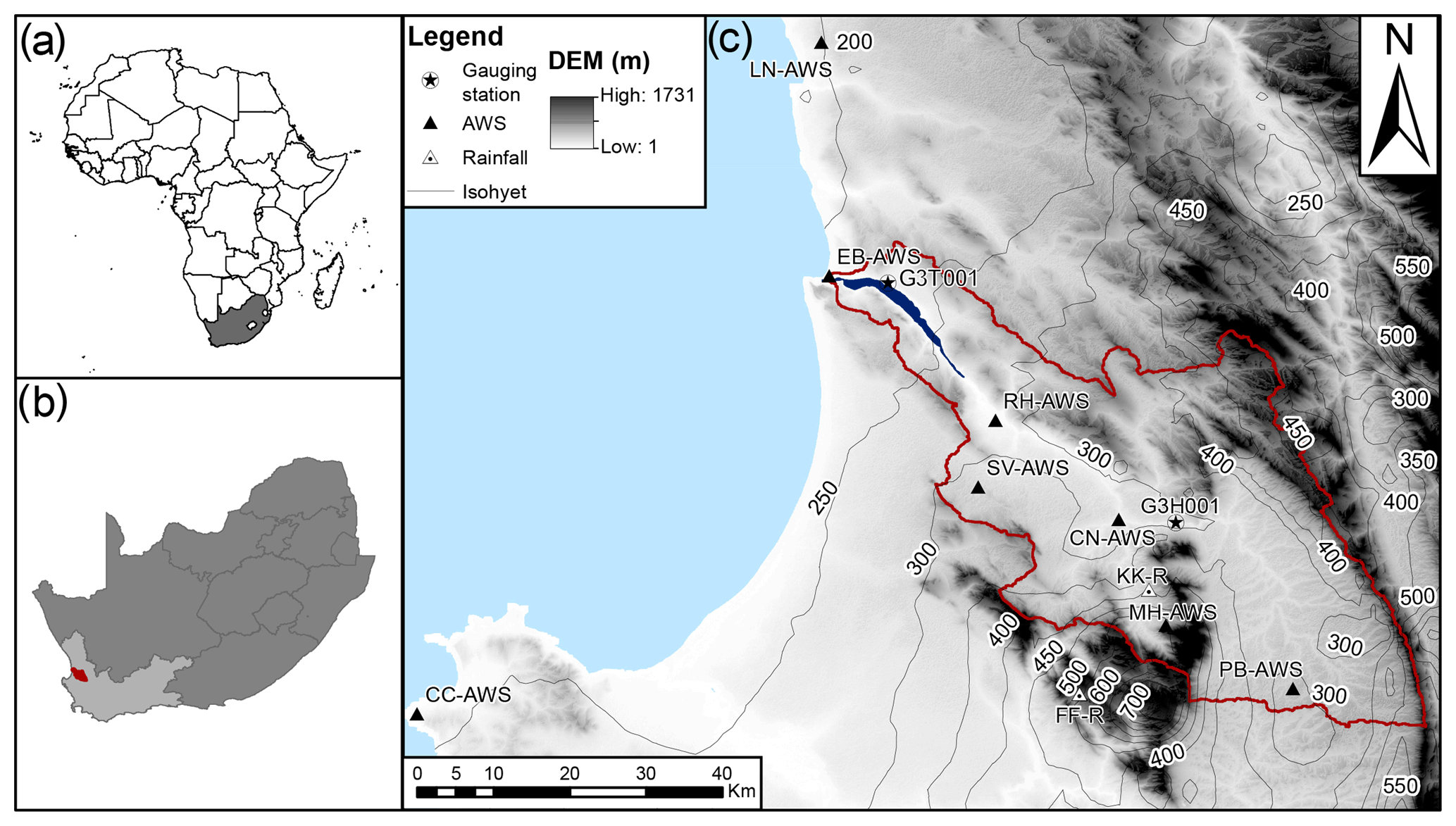
Figure 1 (a) Location of South Africa, (b) the location of the study catchment within the Western Cape and (c) the extent of the Verlorenvlei sub-catchment with the climate stations, gauging station (G3H001), measured lake water level (G3T001) and rainfall isohyets.

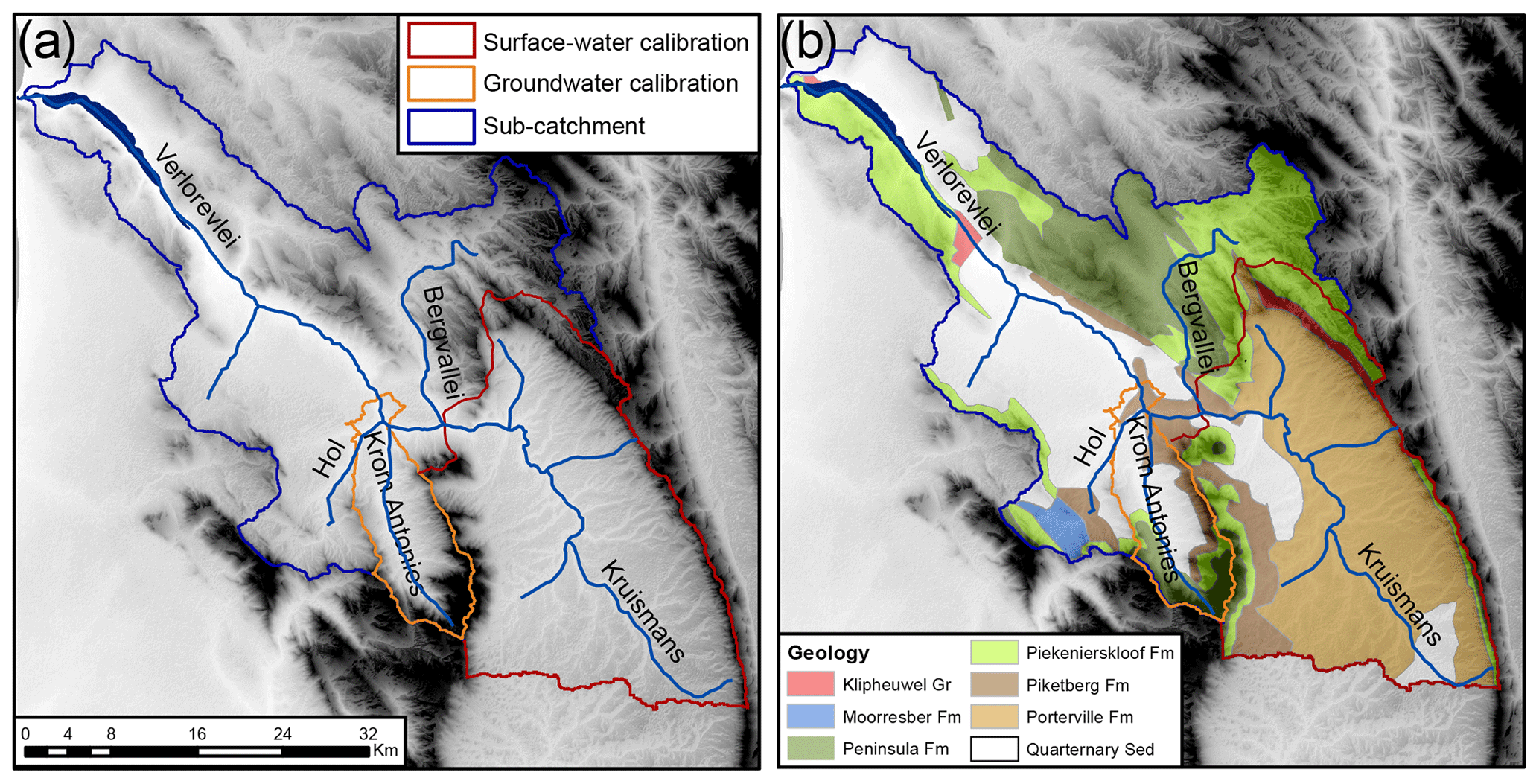
Figure 2 (a) The Verlorenvlei sub-catchment with the surface water calibration tributary (Kruismans) and groundwater calibration tributary (Krom Antonies) and (b) the hydrogeology of the sub-catchment with Malmesbury shale formations (MG; Klipheuwel, Mooresberg, Porterville, Piketberg), Table Mountain Group formations (Peninsula, Piekenierskloof) and Quaternary sediments.

Rainfall for the sub-catchment, recorded over the past 52 years by local farmers at KK-R (Fig. 1), shows large yearly variability (26 %) between the mean annual precipitation (MAP) (411 mm) and measured rainfall (Fig. 3). Where rainfall was greater than 500 mm yr⁻¹ (2006–2010), it is presumed that the lake is supported by a constant influx of streamflow from the feeding tributaries. Recently, where rainfall was less than 50 % of the MAP (2015–2017), concerns over the amount of streamflow required to support the lake have been raised.

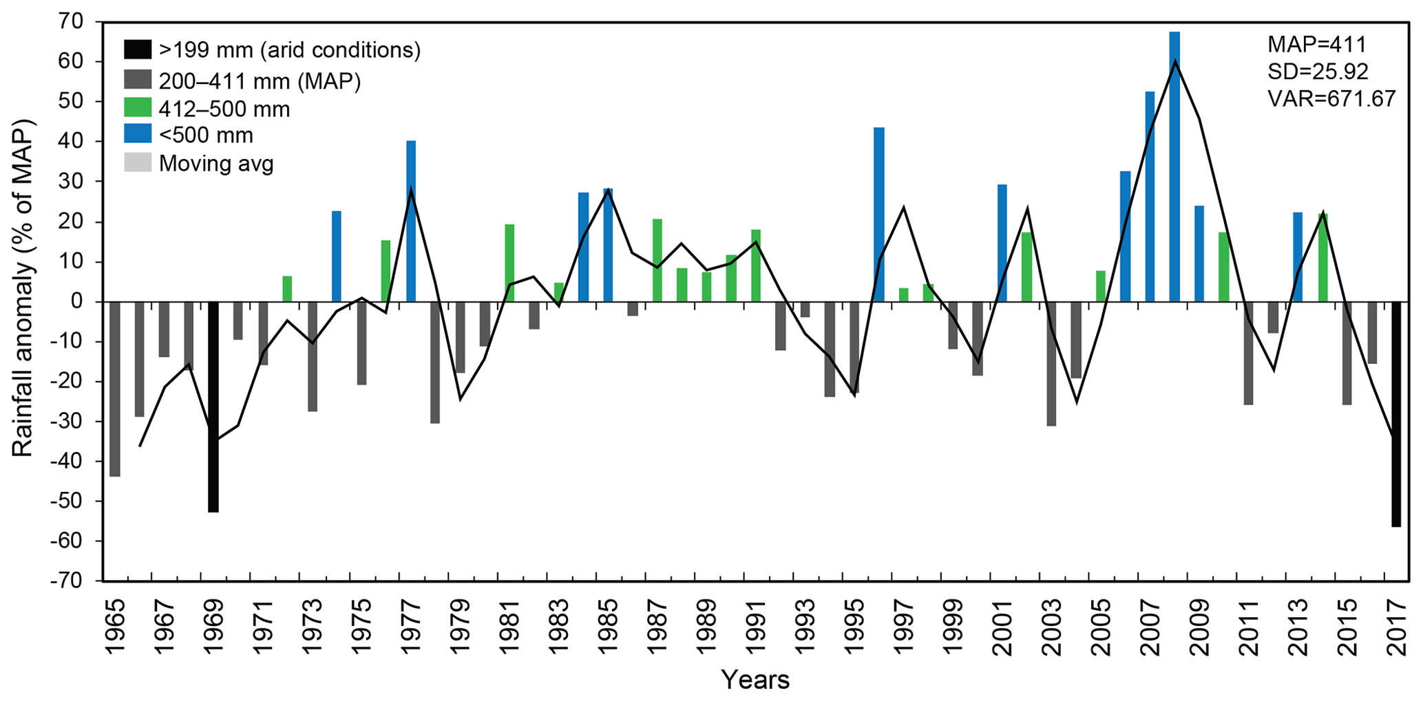
Figure 3 The difference between MAP and measured rainfall (plotted as rainfall anomaly) for 52 years (1965–2017) at location KK-R in the valley of Krom Antonies (after Watson et al., 2018).

While rainfall varies greatly between years in the sub-catchment, it is also spatially impacted by elevational differences. The catchment valley which receives the least MAP, 100–350 mm yr⁻¹ (Lynch, 2004), is between 0 and 350 m a.s.l., and is comprised of Quaternary sediments that vary in texture, although the majority of the sediments in the sub-catchment are sandy in nature. The higher relief mountainous regions of the sub-catchment between 400 and 1300 m a.s.l. receive the highest MAP, 400–800 mm yr⁻¹ (Lynch, 2004), and are mainly comprised of fractured TMG sandstones, (youngest to oldest): the Peninsula, Graafwater (not shown), and Piekernerskloof formations (Fig. 2) (Johnson et al., 2006). Underlying the sandstones and Quaternary sediments are the MG shales, which are comprised of the Mooresberg, Piketberg and Klipheuwel formations (Fig. 2) (Rozendaal and Gresse, 1994). Agriculture is the dominant water user in the sub-catchment with an estimated usage of 20 % of the total recharge (Conrad et al., 2004; DWAF, 2003), with the main food crop being potatoes. The MG shales and Quaternary sediments, which host the secondary and primary aquifers respectively, are frequently used to supplement irrigation during the summer months of the year. During winter, the majority of the irrigation water needed for crop growth is supplied by the sub-catchment tributaries or the lake itself. The impact of irrigation on the lake is still regarded as minimal (Meinhardt et al., 2018), but further investigation is still required. For additional information regarding the study site, refer to Watson et al. (2018) and Conrad et al. (2004).

3 Methodology

In this study, the J2000 coding was adapted to incorporate distributed groundwater components for the model HRUs (Fig. 4). This was done by aligning the MODFLOW recharge estimates and previous studies (Conrad et al., 2004; Miller et al., 2017; Vetger, 1995; Weaver and Talma, 2005; Wu, 2005) with those of J2000, through adjustment of aquifer hydraulic conductivity from the MODFLOW groundwater model of Krom Antonies (Watson, 2018) (Fig. 5). The assigned hydraulic conductivity for each geological formation was thereafter transferred across the entire J2000 model of the sub-catchment. The adaption applied to the groundwater components influenced the proportioning of water routed to runoff and baseflow within the J2000 model. To validate the outputs of the model, an empirical mode decomposition (EMD) (Huang et al., 1998) was applied to compute the proportion of variation in discharge time series that was attributed to high and low water level changes at the sub-catchment outlet. The streamflow estimates were thereafter compared with the lake evaporation demand to understand the sub-catchment water balance.

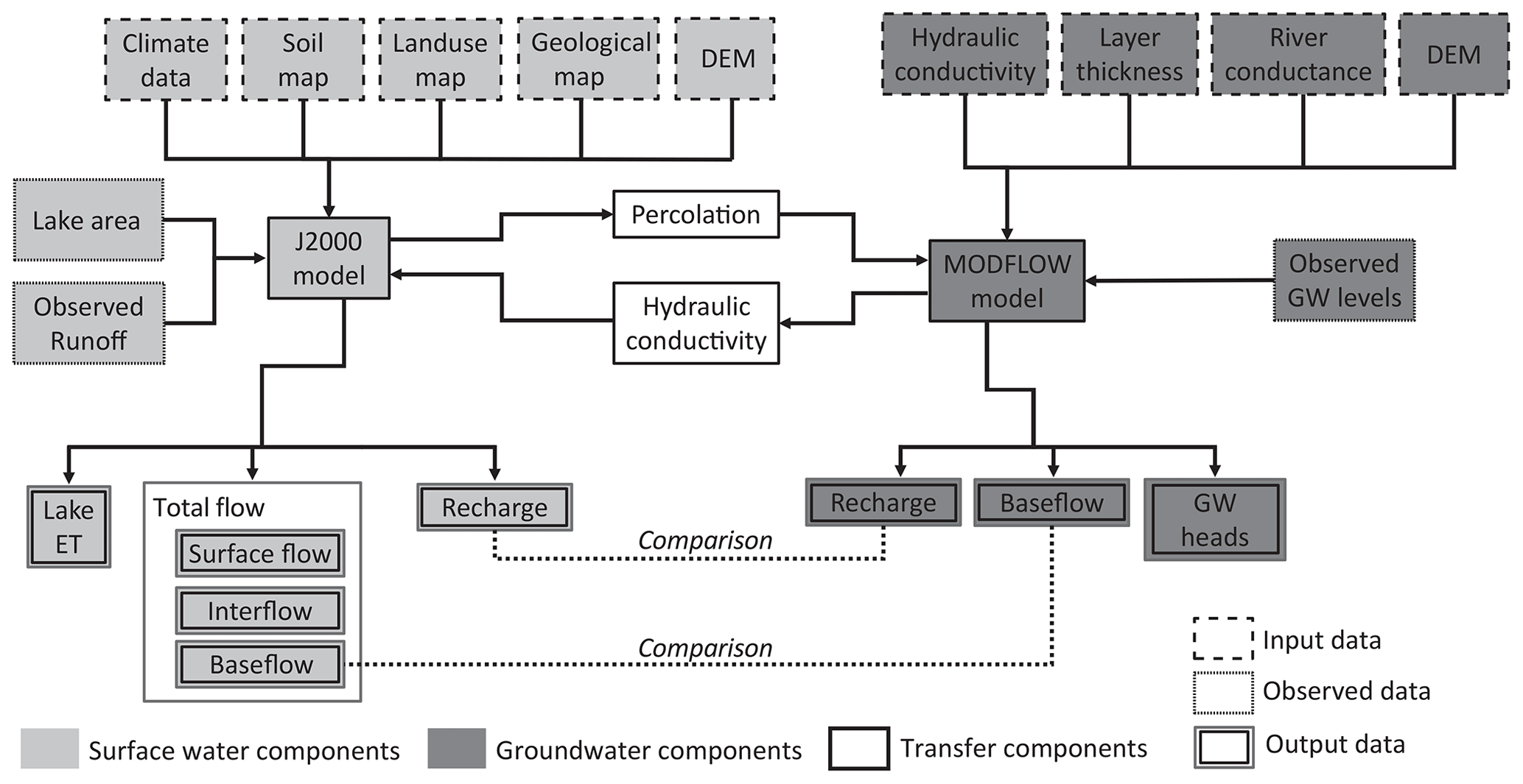
Figure 4 Schematic of the model structure, showing the processors simulated by J2000 and MODFLOW and the components that were transferred from the MODFLOW model.

The J2000 model incorporated distributed climate, soil, land-use and hydrogeological information, with aquifer hydraulic conductivity transferred from MODFLOW as described above (Fig. 4). The measured streamflow was used to both calibrate and validate the model, with the land-use dataset being selected according to the period of measured streamflow. Changes in the recorded lake level were used alongside remote sensing to estimate the lake evaporation rate. The impact of irrigation was not included in the model, as there is not enough information available regarding agricultural water use. This is currently one of the major limitations with the study approach presented here and will be the focus of future work. The HRU delineation, model regionalisation, water balance calculations, lateral and reach routing as well as the lake evaporation procedure are presented. Thereafter the input data for the model, the calibration and validation procedures as well as the EMD protocol used are described.

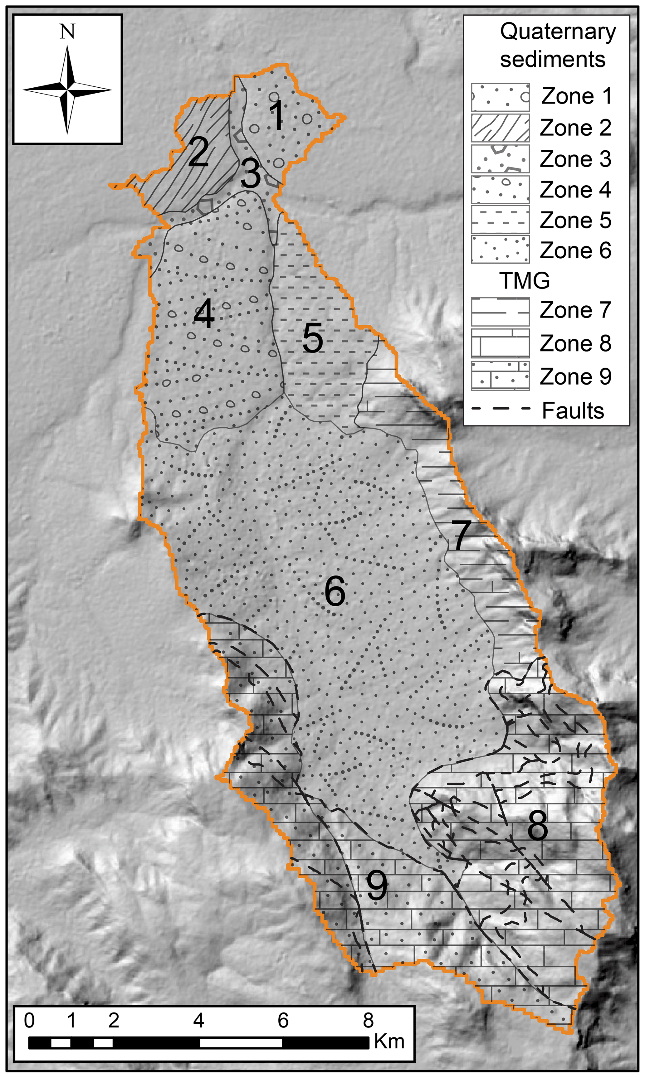
Figure 5 The aquifer hydraulic zones used for the groundwater calibration of J2000 (after Watson, 2018).

3.1 Hydrological response unit delineation

HRUs and stream segments (reaches) are used within the J2000 model for distributed topographic and physiological modelling. In this study, the HRU delineation made use of a digital elevation model, with slope, aspect, solar radiation index, mass balance index and topographic wetness being derived. Before the delineation process, gaps within the digital elevation model were filled using a standard fill algorithm from ArcInfo (Jenson and Domingue, 1988). The AML (ArcMarkupLanguage) automated tool (Pfennig et al., 2009) was used for the HRU delineation, with between 13 and 14 HRUs km⁻² being defined (Pfannschmidt, 2008). After the delineation of HRUs, dominant soil, land-use and geology properties were assigned to each. The hydrological topology was defined for each HRU by identifying the adjacent HRUs or stream segments that received water fluxes.

3.2 Model regionalisation

Rainfall and relative humidity are the two main parameters that are regionalised within the J2000 model. While a direct regionalisation using an inverse-distance method (IDW) and the elevation of each HRU can be applied to rainfall data, the regionalisation of relative humidity requires the calculation of absolute humidity. The regionalisation of rainfall records was applied by defining the number of weather station records available and estimating the influence on the rainfall amount for each HRU. A weighting for each station using the distance of each station to the area of interest was applied to each rainfall record, using an elevation correction factor (Krause, 2001). The relative humidity and air temperature measured at set weather stations were used to calculate the absolute humidity. Absolute humidity was thereafter regionalised using the IDW method, station and HRU elevation. After the regionalisation had been applied, the absolute humidity was converted back to relative humidity through calculation of saturated vapour pressure and the maximum humidity.

3.3 Water balance calculations

The J2000 model is divided into calculations that impact surface water and groundwater processors. The J2000 model distributes the regionalised precipitation (P) calculated for each HRU using a water balance defined as

$$\begin{array}{}\text{(1)}& {\displaystyle }P=R+{\mathrm{Int}}_{\max }+\mathrm{ETR}+\mathrm{\Delta }{\mathrm{Soil}}_{\mathrm{sat}},\end{array}$$

where R is runoff (mm) (RD1 – surface runoff; RD2 – interflow), Int_max is vegetation canopy interception (mm), ETR is “real” evapotranspiration and ΔSoil_sat is change in soil saturation. The surface water processes have an impact on the amount of modelled runoff and interflow, while the groundwater processors influence the upper and lower groundwater flow components.

3.3.1 Surface water components

Potential evaporation (ETP) within the J2000 model is calculated using the Penman–Monteith equation. Before evaporation was calculated for each HRU, interception was subtracted from precipitation using the leaf area index and leaf storage capacity for vegetation (a_rain) (Table S1 in the Supplement). Evaporation within the model considers several variables that influence the overall modelled evaporation. Firstly, evaporation is influenced by a slope factor, which was used to reduce ETP based on a linear function. Secondly, the model assumed that vegetation transpires until a particular soil moisture content where ETP is reached, after which modelled evaporation was reduced proportionally to the ETP, until it becomes zero at the permanent wilting point.

The soil module in the J2000 model is divided up into processing and storage units. Processing units in the soil module include soil–water infiltration and evapotranspiration, while storage units include middle pore storage (MPS), large pore storage (LPS) and depression storage. The infiltrated precipitation was calculated using the relative saturation of the soil and its maximum infiltration rate (SoilMaxInfSummer and SoilMaxInfWinter) (Table S1). Surface runoff was generated when the maximum infiltration threshold was exceeded. The amount of water leaving LPS, which can contribute to recharge, was dependent on soil saturation and the filling of LPS via infiltrated precipitation. Net recharge (R_net) was estimated using the hydraulic conductivity (SoilMaxPerc), the outflow from LPS (LPS_out) and the slope (slope) of the HRU according to

$$\begin{array}{}\text{(2)}& {\displaystyle }{R}_{\mathrm{net}}={\mathrm{LPS}}_{\mathrm{out}}\times (\mathrm{1}-\tan \left(\mathrm{slope}\right)\mathrm{SoilMaxPerc}).\end{array}$$

The hydraulic conductivity, SoilMaxPerc and the adjusted LPS_out were thereafter used to calculate interflow (IT_f) according to

$$\begin{array}{}\text{(3)}& {\displaystyle }{\mathrm{IT}}_f={\mathrm{LPS}}_{\mathrm{out}}\times \left(\tan \left(\mathrm{slope}\right)\mathrm{SoilMaxPerc}\right),\end{array}$$

with the interflow calculated representing the sub-surface runoff component RD2 and routed as runoff within the model.

3.3.2 Groundwater components

The J2000 model for the Verlorenvlei sub-catchment was set up with two different geological reservoirs: (1) the primary aquifer (upper groundwater reservoir – RG1), which consists of Quaternary sediments with a high permeability; and (2) the secondary aquifer (lower groundwater reservoir – RG2), made up of MG shales and TMG sandstones (Table 1).

Table 1 The J2000 hydrogeological parameters RG1_max, RG2_max, RG1_k, RG2_Kf_geo and depthRG1 assigned to the primary and secondary aquifer formations for the Verlorenvlei sub-catchment.

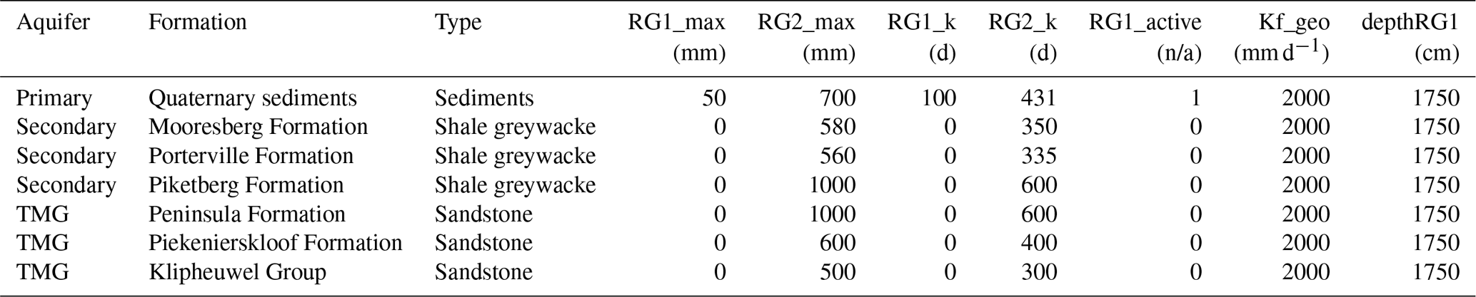
n/a: not applicable.

The model therefore considered two baseflow components, a fast one from RG1 and a slower one from RG2. The filling of the groundwater reservoirs was done by net recharge, with emptying of the reservoirs possible by lateral subterranean runoff as well as capillary action in the unsaturated zone. Each groundwater reservoir was parameterised separately using the maximum storage capacity (maxRG1 and maxRG2) and the retention coefficients for each reservoir (recRG1 and recRG2). The outflow from the reservoirs was determined as a function of the actual filling (actRG1 and actRG2) of the reservoirs and a linear drain function. Calibration parameters recRG1 and recRG2 are storage residence time parameters. The outflow from each reservoir was defined as

$$\begin{array}{}\text{(4)}& {\displaystyle }& {\displaystyle }\mathrm{OutRG}\mathrm{1}={\displaystyle \frac{\mathrm{1}}{\mathrm{gwRG}\mathrm{1}\mathrm{Fact}\times \mathrm{recRG}\mathrm{1}}}\times \mathrm{actRG}\mathrm{1},\text{(5)}& {\displaystyle }& {\displaystyle }\mathrm{OutRG}\mathrm{2}={\displaystyle \frac{\mathrm{1}}{\mathrm{gwRG}\mathrm{2}\mathrm{Fact}\times \mathrm{recRG}\mathrm{2}}}\times \mathrm{actRG}\mathrm{2},\end{array}$$

where OutRG1 is the outflow from the upper reservoir, OutRG2 is the outflow from the lower reservoir and gwRG1Fact ∕ gwRG2Fact are calibration parameters for the upper and lower reservoirs used to determine the outflow from each reservoir. To allocate the quantity of net recharge between the upper (RG1) and lower (RG2) groundwater reservoirs, a calibration coefficient gwRG1RG2sdist was used to distribute the net recharge for each HRU using the HRU slope. The influx of groundwater into the shallow reservoir (inRG1) was defined as

$$\begin{array}{}\text{(6)}& {\displaystyle }\mathrm{inRG}\mathrm{1}=R_{\mathrm{net}}\times (\mathrm{1}-(\mathrm{1}-\tan \left(\mathrm{slope}\right)\left)\right)\times \mathrm{gwRG}\mathrm{1}\mathrm{RG}\mathrm{2}\mathrm{sdist}.\end{array}$$

The influx of net recharge into the lower groundwater reservoir (inRG2) was defined as

$$\begin{array}{}\text{(7)}& {\displaystyle }\mathrm{inRG}\mathrm{2}=R_{\mathrm{net}}\times (\mathrm{1}-\tan (\mathrm{slope}\left)\right)\times \mathrm{gwRG}\mathrm{1}\mathrm{RG}\mathrm{2}\mathrm{sdist},\end{array}$$

with the combination of OutRG1 and OutRG2 representing the baseflow component that is routed as an outflow from the model.

3.4 Lateral and reach routing

Lateral routing was responsible for water transfer within the model and included HRU influxes and discharge through routing of cascading HRUs from the upper catchment to the exit stream. HRUs were either able to drain into multiple receiving HRUs or into reach segments, where the topographic ID within the HRU dataset determined the drain order. The reach routing module was used to determine the flow within the channels of the river using the kinematic wave equation and calculations of flow according to Manning and Strickler. The river discharge was determined using the roughness coefficient of the stream (Manning roughness), the slope and width of the river channel and calculations of flow velocity and hydraulic radius done during model simulations.

3.5 Calculations of lake evaporation rate

The lake evaporation rate was based on the ETP calculated by J2000 and an estimated lake surface area. The lake was modelled as a unique HRU (water as the land-cover type), with a variable area which was estimated using remote sensing data from Landsat 8 and Sentinel-2 and the measured lake water level at G3T001 (Fig. 1). To infill lake surface area when remote sensing data were not available, a relationship was created between the estimated lake's surface area and the measured water level between 2015 and 2017. Where lake water level data were not available (before 1999), an average long-term monthly value was used for the lake evaporation calculations.

3.6 J2000 input data

3.6.1 Surface water parameters

Rainfall, wind speed, relative humidity, solar radiation and air temperature were monitored by automated weather stations (AWSs) within and outside of the study catchment (Fig. 1). Of the climate and rainfall data used during the surface water modelling (Watson et al., 2018), data were sourced from seven AWSs, of which four stations were owned by the South African Weather Service (SAWS) and three by the Agricultural Research Council (ARC). Two stations that were installed for the surface water modelling, namely Moutonshoek (M-AWS) and Confluence (CN-AWS), were used for climate and rainfall validation due to their short record length. Additional rainfall data collected by farmers at high elevation at location FF-R and within the middle of the catchment at KK-R were used to improve the climate and rainfall network density.

Land-use classification

The vegetation and land-use dataset that was used for the sub-catchment (CSIR, 2009) included five different land-use classes: (1) wetlands and waterbodies, (2) cultivated (temporary, commercial, dryland), (3) shrubland and low fynbos, (4) thicket, bushveld, bush clumps and high fynbos and (5) cultivated (permanent, commercial, irrigated). Each different land-use class was assigned an albedo, root depth and seal grade value based on previous studies (Steudel et al., 2015) (Table S2). The leaf area index (LAI) and vegetation height vary by growing season with different values of each for the particular growing season. While surface resistance of the land use varied monthly within the model, the values only vary significantly between growing seasons.

Soil dataset

The Harmonized World Soil Database (HWSD) v1.2 (Batjes et al., 2012) was the input soil dataset, with nine different soil forms within the sub-catchment (Table S3). Within the HWSD, soil depth, soil texture and granulometry were used to calculate and assign soil parameters within the J2000 model. MPS and LPS, which differ in terms of the soil structure and pore size, were determined in Watson et al. (2018) using pedotransfer functions within the HYDRUS model (Table S3).

Streamflow and water levels

Streamflow, measured at Department of Water Affairs (DWA) gauging station G3H001 between 1970 and 2009, at the outlet of Kruismans tributary (Het Kruis) (Figs. 1 and 3), was used for surface water calibration. The G3H001 two-stage weir was able to record a maximum flow rate of 3.68 m³ s⁻¹ due to the capacity limitations of the structure. After 2009, the G3H001 structure was decommissioned due to structural damage, although repairs are expected in the near future due to increasing concerns regarding the influx of freshwater into the lake. Water levels measured at the sub-catchment outlet at DWA station G3T001 (Fig. 1) between 1994 and 2018 were used for EMD filtering.

3.6.2 Groundwater parameters

Net recharge and hydraulic conductivity

The hydraulic conductivity values used for the groundwater component adaptation were collected from detailed MODFLOW modelling of Krom Antonies tributary (Fig. 5) (Watson, 2018). The net recharge and aquifer hydraulic conductivity for Krom Antonies tributary were estimated through PEST autocalibration using hydraulic conductivities from previous studies (SRK, 2009; Hartnady and Hay, 2000) and potential recharge estimates (Watson et al., 2018).

Hydrogeology

Within the hydrogeological dataset, parameters assigned include maximum storage capacity (RG1 and RG2), storage coefficients (RG1 and RG2), the minimum permeability/maximum percolation (Kf_geo of RG1 and RG2) and depth of the upper groundwater reservoir (depthRG1). The maximum storage capacity was determined using an average thickness of each aquifer and the total number of voids and cavities, where the primary aquifer thickness was assumed to be between 15 and 20 m (Conrad et al., 2004) and the secondary aquifer between 80 and 200 m (SRK, 2009). The maximum percolation of the different geological formations was assigned hydraulic conductivities using the groundwater model for Krom Antonies sub-catchment (Watson, 2018). The J2000 geological formations were assigned conductivities to modify the maximum percolation value to ensure internal consistency with recharge values calculated using MODFLOW (Table 1).

3.7 J2000 model calibration

3.7.1 Model sensitivity

The J2000 sensitivity analysis for Verlorenvlei sub-catchment was presented in Watson et al. (2018), and therefore only a short summary is presented here. In this study, parameters that were used to control the ratio of interflow to percolation were adjusted, which in the J2000 model include slope (SoilLatVertDist) and max percolation values. The sensitivity analysis conducted by Watson et al. (2018) showed that for high-flow conditions (E2) (Nash–Sutcliffe efficiency in its standard squared form), model outputs are most sensitive to the slope factor, while for low-flow conditions (E1) (modified Nash–Sutcliffe efficiency in a linear form), the model outputs were most sensitive to the maximum infiltration rate of the soil (i.e. the parameter maxInfiltrationWet) (Fig. S1). The max percolation was moderately sensitive during wet and dry conditions, and together with the slope factor controlled the interflow-to-percolation proportioning that was calibrated in this study.

3.7.2 Surface water calibration

The surface water parameters of the model were calibrated for Kruismans tributary (688 km²) (Fig. 3) using the gauging data from G3H001 (Fig. 6 and Table 1). The streamflow data used for the calibration were between 1986 and 1993, with model validation between 1994 and 2007 (Fig. 6). This specific calibration period was selected due to the wide range of different runoff conditions experienced at the station, with both low- and high-flow events being recorded. For the calibration, the modelled discharge was manipulated in the same fashion, with a DT (discharge table) limit of 3.68 m³ s⁻¹, so that the tributary streamflow behaved as measured discharge.

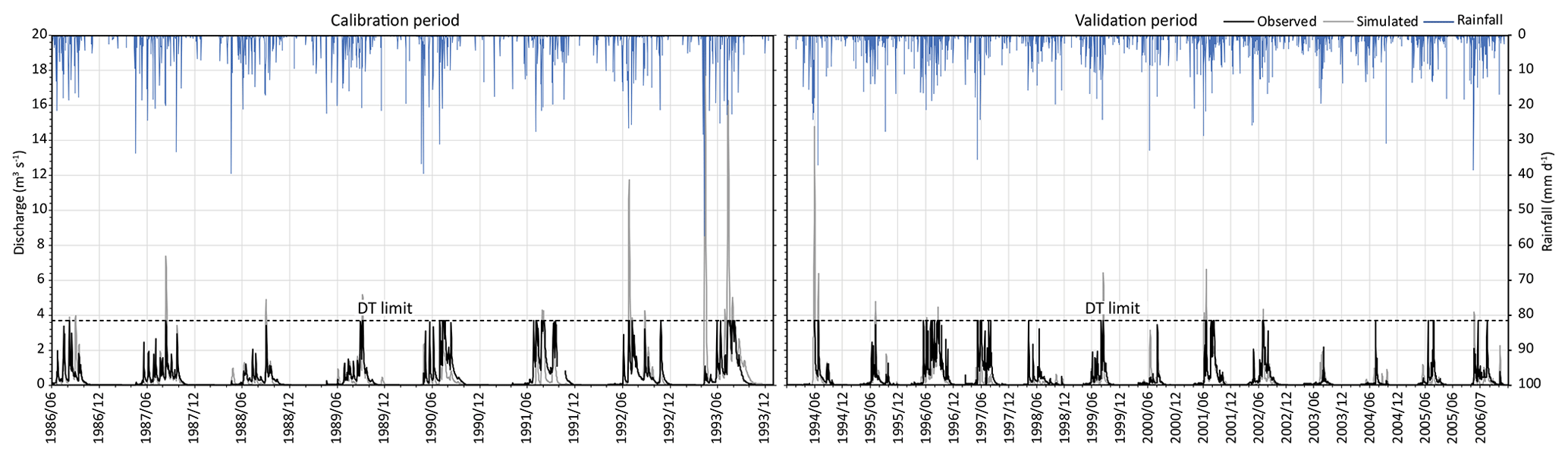
Figure 6 The surface water calibration (1986–1993) and validation (1994–2006) of the J2000 model using gauging data from the G3H001.

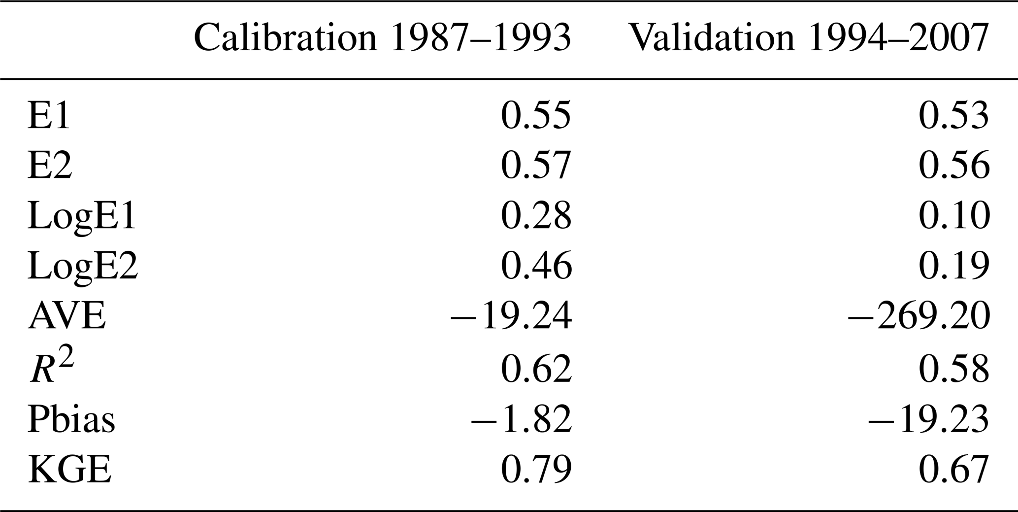
An automated model calibration was performed using the Nondominating Sorting Genetic Algorithm II (NSGA-II) multi-objective optimisation method (Deb et al., 2002) with 1024 model runs being performed. Narrow ranges of calibration parameters (FC_Adaptation, AC_Adaptation, soilMAXDPS, gwRG1Fact and gwRG2Fact) were chosen to (1) ensure that the modelled recharge from J2000 was within an order of magnitude of recharge from the MODFLOW model and previous studies; and (2) achieve a representative sub-catchment hydrograph. As objective functions, Nash–Sutcliffe efficiency based on absolute differences (E1) and squared differences 2 (E2) as well as the average bias in % (Pbias) were utilised for the calibration (Krause et al., 2005) (Table 2). The choice of the optimised parameter set was made to ensure that E2 was better than 0.57 (the best value was 0.57) and the Pbias better than 5 % (Table 1). From the automated calibration, 308 parameter sets were determined, with the best E1 being chosen to ensure that the model is representative of low-flow conditions (Table 1).

3.7.3 Model validation

Observed vs. modelled streamflow

For the surface water model validation, the streamflow records between 1994 and 2007 were used, where Nash–Sutcliffe efficiencies (E1 and E2) were reported. The Pbias was also used as an objective function to report the model performance by comparison between measured and modelled streamflow (Table 2). Although gauging station limitations resulted in good objective functions from the model, the performance of objective functions E1 and E2 and Pbias decreased between the validation and calibration periods (Table 2). During the calibration period there was a good fit between modelled and measured streamflow (Pbias $=-\mathrm{1.82}$), with a significant difference between modelled and measured streamflow during the validation period (Pbias $=-\mathrm{19.2}$). The calibration was performed over a wet cycle (1986–1997), which resulted in a more common occurrence of streamflow events that exceeded 3.68 m³ s⁻¹, thereby reducing the number of calibration points. In contrast, the validation was performed over a dry cycle (1997–2007), which resulted in more data points as few streamflow events exceeded 3.68 m³ s⁻¹.

Table 2 Value of the objective functions E1 and E2, logarithmic versions of E1 and E2, absolute volume error (AVE), coefficient of determination (R²), Pbias and Kling–Gupta efficiency (KGE) (Gupta et al., 2009) for surface water calibration (1987–1993) and validation (1994–2007).

The J2000 and MODFLOW recharge estimates

With adjustment of hydraulic conductivities from MODFLOW to J2000 it was possible to converge the net recharge estimates between 1.3 % with a range of recharge of 0.65 %–10.03 % for J2000 and 0.3 %–11.40 % for MODFLOW. Recharge estimates from previous studies of the primary aquifer indicate recharge rates of 0.2 %–3.4 % (Conrad et al., 2004) and 8 % (Vetger, 1995), and for the TMG aquifer 13 % (Wu, 2005), 27 % (Miller et al., 2017) and 17.4 % (Weaver and Talma, 2005) of MAP. J2000 estimates had an average value of 5.30 %, while MODFLOW was 5.20 % for the eight hydraulic zones of Krom Antonies. The coefficient of determination (R²) between net recharge from J2000 and MODFLOW was 0.81. Across the entire dataset J2000 overestimated groundwater recharge by 2.75 % relative to MODFLOW, although the coefficient of determination produced an R² of 0.92, which is better than during the validation period.

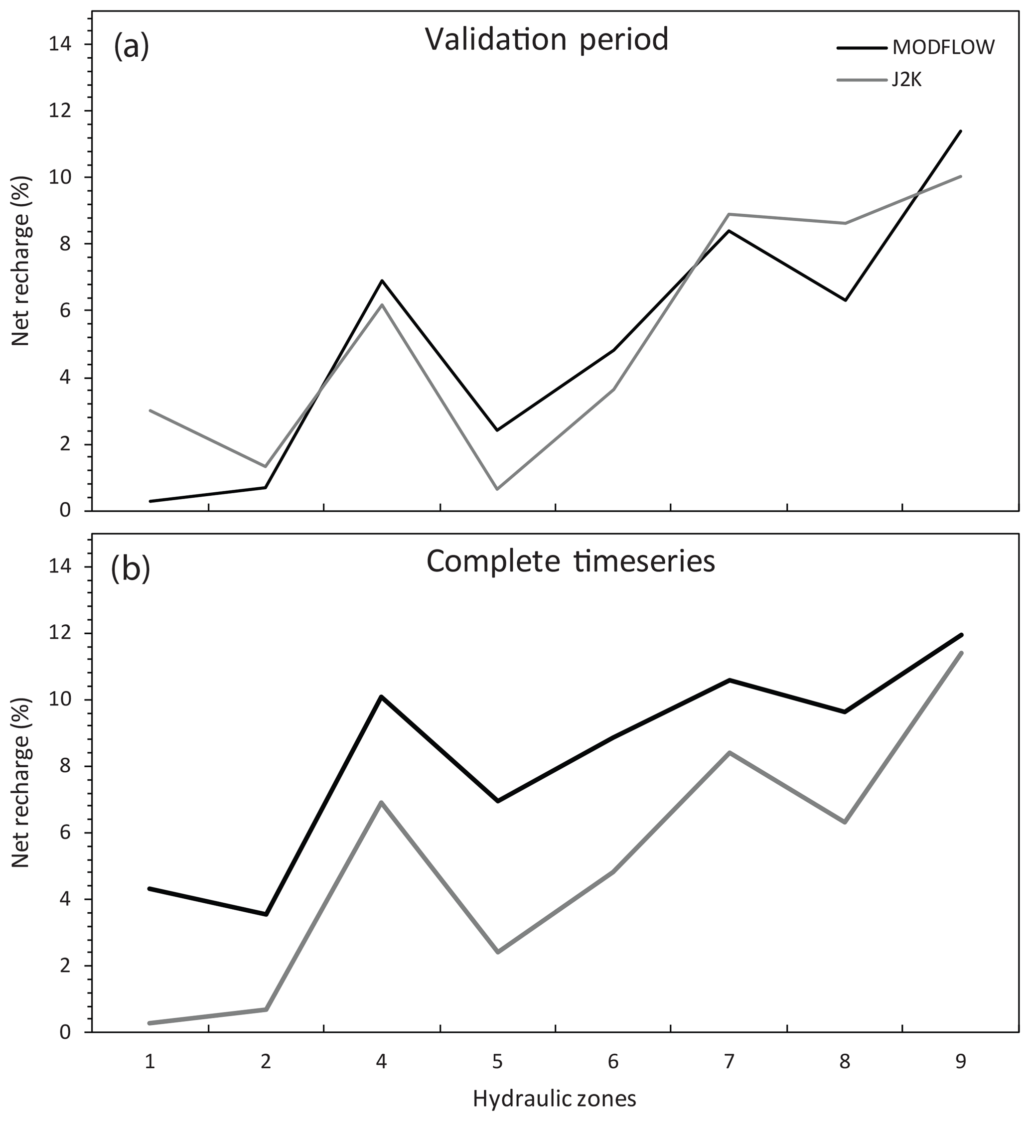
Figure 7 The groundwater calibration for each hydraulic zone with (a) net recharge for J2000 and MODFLOW during the model calibration (2016) and (b) the net recharge deviation between MODFLOW and J2000 across the entire modelling time step (1986–2017).

3.8 EMD filtering

To account for missing streamflow data between 2007 and 2017, an empirical mode decomposition (EMD) (Huang et al., 1998) was applied to the measured water level data at the sub-catchment outlet (G3T001) (Fig. 1) between 1994 and 2018 (Fig. 8a). EMD is a method for the decomposition of non-linear and non-stationary signals into sub-signals of varying frequency, so-called intrinsic mode functions (IMFs), and a residuum signal. By removing one or more IMFs or the residuum signal, certain frequencies (e.g. noise) or an underlying trend can be removed from the original time-series data. This approach was successfully applied to the analysis of river runoff data (Huang et al., 2009) and forecasting of hydrological time series (Kisi et al., 2014). In this study, EMD filtering was used to remove high-frequency sub-signals from simulated runoff and measured water level data to compare the more general seasonal variations of both signals (Fig. 8b).

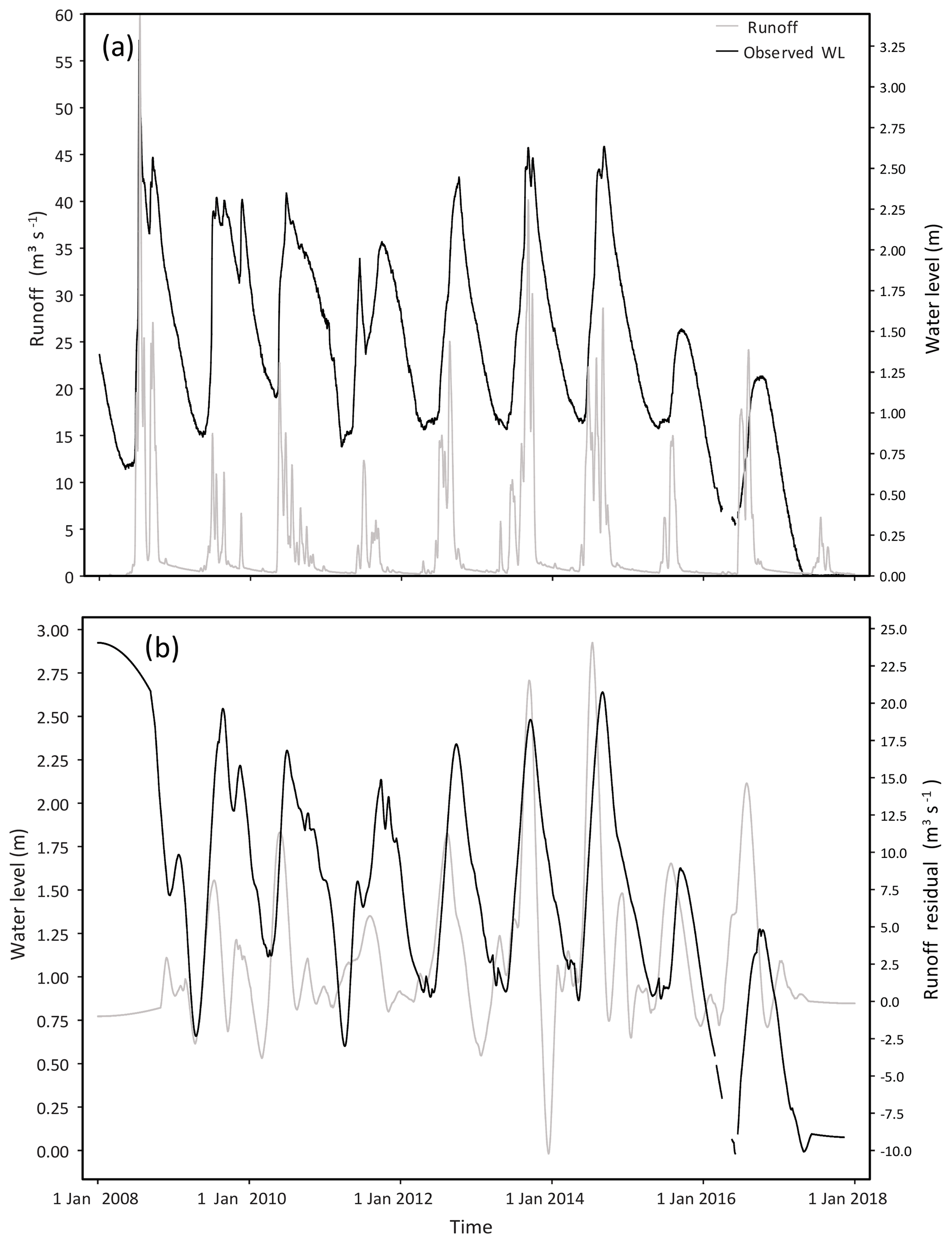
Figure 8 (a) The water level fluctuations at station G3T001 with modelled runoff and (b) the EMD filtering showing the variation in discharge time series attributed to a water level change at the station.

4 Results

The J2000 model was used to simulate both runoff and baseflow, with runoff being comprised of direct surface runoff (RD1) and interflow (RD2) and baseflow simulated from the primary (RG1) and secondary (RG2) aquifers. Below, the results of the modelled streamflow and baseflow are presented, along with the total flow contribution of each tributary, the runoff-to-baseflow proportioning and stream exceedance probabilities. The coefficient of variation (CV) was used to determine the streamflow variability of each tributary, while the baseflow index (BFI) was used to determine the baseflow and runoff proportion.

4.1 Streamflow and baseflow

Streamflow for the sub-catchment shows two distinctively wet periods (1987–1996 and 2008–2017) separated by a dry period (1997–2007) (Fig. 9). Yearly sub-catchment rainfall volumes between 1987 and 1996 were between 288 and 492 mm yr⁻¹, with an average of 426 mm yr⁻¹ and a standard deviation (SD) of 51 mm yr⁻¹. For this period, average yearly streamflow was 1.4 m³ s⁻¹, with an average baseflow contribution of 0.63 m³ s⁻¹. The modelled streamflow reached a maximum of 48 m³ s⁻¹ in 1993, where 5 m³ s⁻¹ of baseflow was generated after 58 mm of rainfall was received. Between 1997 and 2007 (dry period) sub-catchment yearly rainfall was between 222 and 394 mm yr⁻¹ with an average of 326 mm yr⁻¹ and a SD of 69 mm yr⁻¹ (Fig. 9). For this same period, average yearly streamflow was 0.44 m³ s⁻¹, with an average baseflow contribution of 0.18 m³ s⁻¹. The modelled streamflow reached a maximum of 11 m³ s⁻¹ in 2002, with a baseflow contribution of 2.5 m³ s⁻¹ after 28 mm of rainfall was received. During the second wet period between 2008 and 2017 sub-catchment yearly rainfall was between 231 and 582 mm yr⁻¹ with an average of 442 mm yr⁻¹ and a SD of 112 mm yr⁻¹ (Fig. 9). Over this same period, average yearly streamflow was 2.5 m³ s⁻¹ with an average baseflow contribution of 1.3 m³ s⁻¹. The modelled streamflow reached a maximum of 52 m³ s⁻¹ in 2008, with 13 m³ s⁻¹ of baseflow generated after two consecutive rainfall events each of 25 mm.

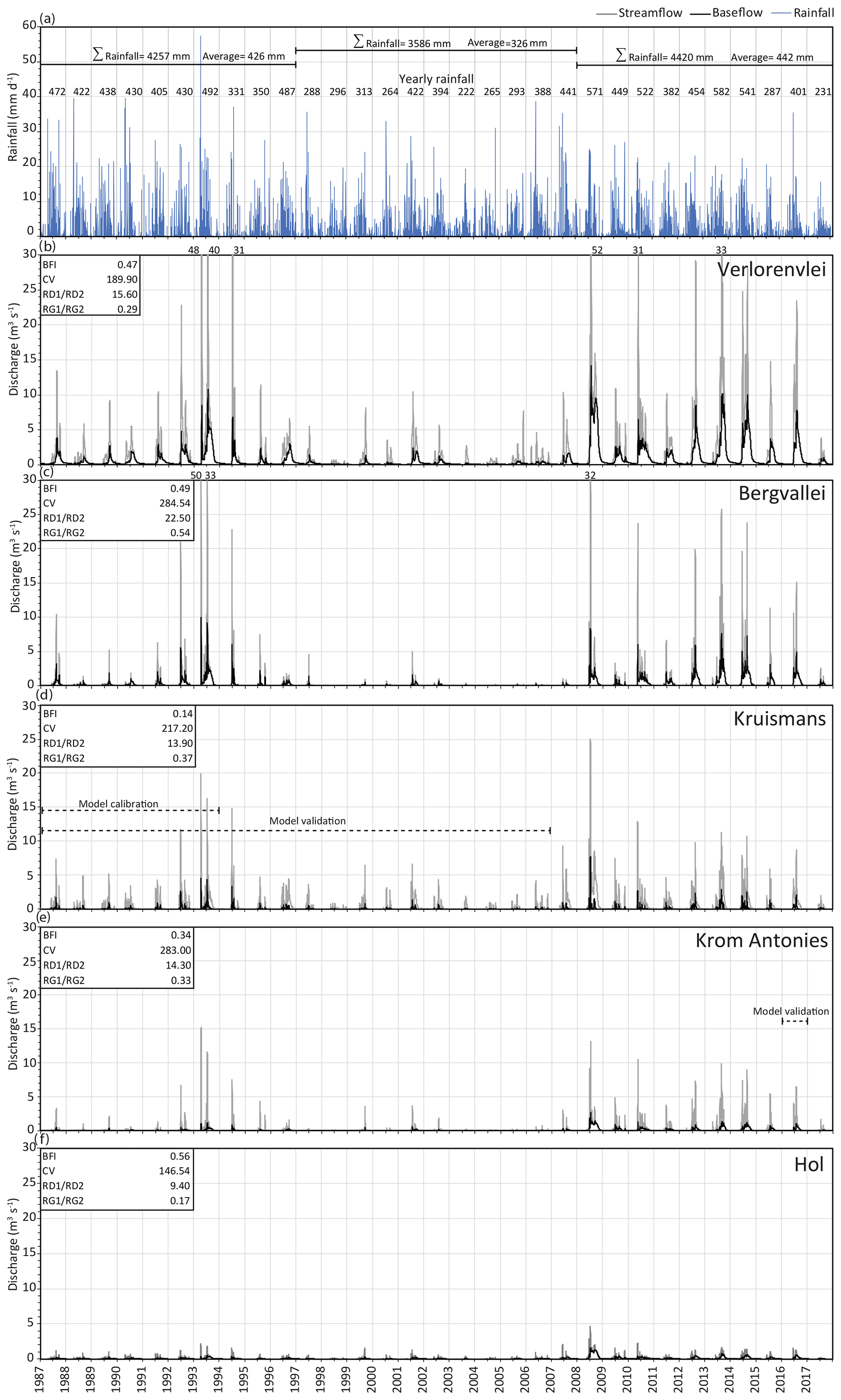
Figure 9 (a) Average sub-catchment rainfall between 1987 and 2017 showing wet cycles (1987–1997 and 2008–2017) and a dry cycle (1997–2007). Modelled streamflow and baseflow inflows for the (b) Verlorenvlei, (c) Bergvallei, (d) Kruismans, (e) Krom Antonies and (f) Hol tributaries with estimated BFI, CV, RD1/RD2, and RG1/RG2.

4.2 Tributary contributions

The four main feeding tributaries (Bergvallei, Kruismans, Hol and Krom Antonies) together contribute 81 % of streamflow for the Verlorenvlei, with the additional 19 % from small tributaries near Redelinghuys (Fig. 10). Kruismans contributes most of the total streamflow at 32 % but only 15 % of the area-weighted contribution, as its sub-catchment is the largest of the four tributaries at 688 km² (Fig. 10). Bergvallei with a sub-catchment of 320 km² contributes 29 % of the total flow with an area-weighted contribution of 28 %. Krom Antonies has the largest area-weighted contribution of 30 % due to its small size (140 km²) in comparison to the other tributaries, although Krom Antonies contributes only 13 % of the total flow (Fig. 10). Hol sub-catchment at 126 km² makes up the smallest contribution to the total flow of only 7 %, but has a weighted contribution of 17 % (Fig. 10).

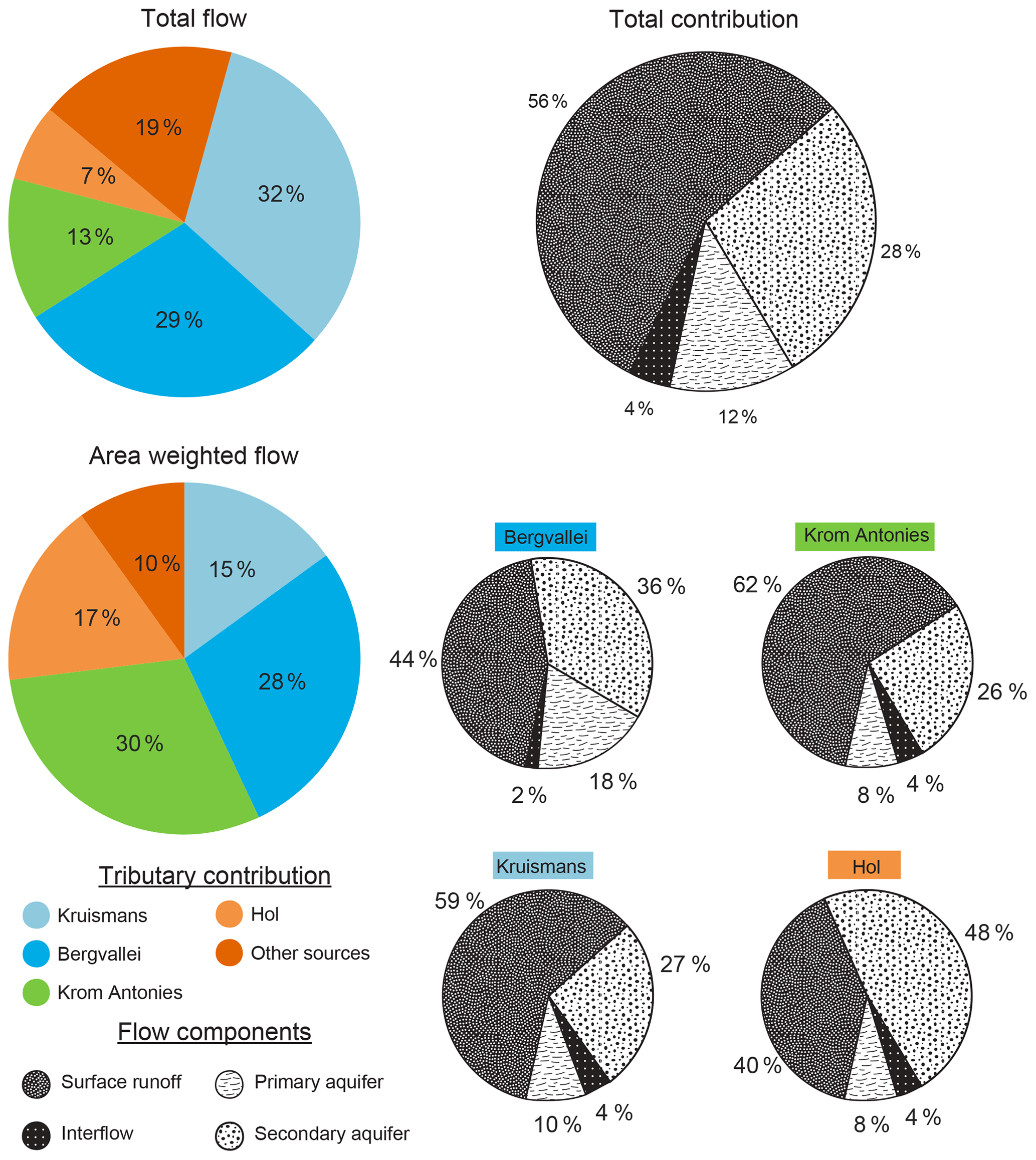
Figure 10 The Verlorenvlei reserve flow contributions (total flow and area-weighted flow) of Kruismans, Bergvallei, Krom Antonies and Hol as well as flow component separation into surface runoff (RD1), interflow (RD2), primary aquifer flow (RG1) and secondary aquifer flow (RG2).

4.3 Flow variability

Streamflow that enters Verlorenvlei has a large daily variability with a CV of 189.90 (Fig. 9). This is mainly due to high streamflow variability from Kruismans (32 %) with a CV of 217.20, which is the major total flow contributor (Fig. 10). Bergvallei and Krom Antonies, which both have high streamflow variability with CV values of 284.54 and 283.00 respectively (Fig. 9), further contribute to the high variability of streamflow that enters the lake. While Hol reduces the overall streamflow variability with a CV of 146.54, it is a minor total flow contributor (7 %) and therefore does not reduce the overall streamflow variability significantly (Fig. 10).

Streamflow that enters Verlorenvlei is dominated by surface runoff which makes up 56 % of total flow, with groundwater and interflow contributing 40 % and 4 % respectively (Fig. 10). The large surface runoff dominance in streamflow entering the lake is due to a high surface runoff contribution from Kruismans and Krom Antonies, which contribute 26 % of total flow from surface runoff. However, for Bergvallei and Hol, surface runoff contributions are less dominant, with 16 % of the total, while the total groundwater contribution is 20 % from these tributaries. Across all four tributaries, the secondary aquifer is the dominant baseflow component, with 28 % of total flow, with the primary aquifer contributing 12 %. Bergvallei and Kruismans contribute the majority of primary aquifer baseflow, with 8 % of the total. The secondary aquifer baseflow is mainly contributed by Kruismans and Bergvallei, where together 18 % of the total is received. Interflow across the four tributaries is uniformly distributed, with 0.3 %–1 % of the total flow being contributed from each tributary.

4.4 Flow exceedance probabilities

The flow exceedance probability, which is a measure of how often a given flow is equalled or exceeded, was calculated for each of the tributaries as well as the lake water body. The results for the flow exceedance probabilities include flow volumes which are exceeded 95 %, 75 %, 50 %, 25 % and 5 % of the time. The 95 percentile corresponds to a lake inflow of 0.054 m³ s⁻¹ or 4702 m³ d⁻¹, with between 0.001 and 0.004 m³ s⁻¹ from the feeding tributaries (Fig. 11 and Table 3). The 75-percentile flow, which is exceeded 3∕4 of the time, corresponds to an inflow of 0.119 m³ s⁻¹ or 10 303 m³ d⁻¹, with between 0.005 and 0.015 m³ s⁻¹ from the feeding tributaries. Average (50-percentile) streamflow flowing into the Verlorenvlei is 0.237 m³ s⁻¹ or 20 498 m³ d⁻¹, with between 0.010 and 0.035 m³ s⁻¹ from the feeding tributaries. The 25-percentile flow, which is exceeded 1∕4 of the time, corresponds to a lake inflow of 1067 m³ s⁻¹ or 92 204 m³ d⁻¹, with between 0.044 and 0.291 m³ s⁻¹ from the feeding tributaries. The lake inflows that are exceeded 5 % of the time correspond to 6.939 m³ s⁻¹ or 599 535 m³ d⁻¹, with between 0.224 and 2.49 m³ s⁻¹ from the feeding tributaries.

Figure 11 The streamflow exceedance percentiles and evaporation demand of the Verlorenvlei reserve, with the contributions from each feeding tributary.

Table 3 The streamflow exceedance percentiles and lake evaporation demand for the Verlorenvlei reserve, with the contributions from Kruismans, Bergvallei, Krom Antonies and Hol (m³ s⁻¹ and m³ d⁻¹).

5 Discussion

The adaptation of the J2000 rainfall–runoff model was used to understand the flow contributions of the main feeding tributaries, the proportioning of baseflow-to-surface runoff as well as how often the inflows exceed the lake evaporation demand. Before a comparison with previous baseflow estimates can be made and the impact of evaporation on the lake reserve understood, the model limitations and catchment flow dynamics must also be assessed.

5.1 Model limitations and performance

A major limitation facing the development and construction of comprehensive modelling systems in sub-Saharan Africa is the availability of appropriate climate and streamflow data. For this study, while there was access to over 20 years of streamflow records, the station was only able to measure a maximum of 3.68 m³ s⁻¹, which hindered calibration of the model for high-flow events. As such, the confidence in the model's ability to simulate high streamflow events using climate records is limited. While the availability of measured data is a limitation that could affect the modelled streamflow, discontinuous climate records also hindered the estimations of long time-series streamflow.

Over the course of the 31-year modelling period, a number of climate stations used for regionalisation were decommissioned and were replaced by stations in different areas. This required adaption of climate regionalisation for simulations over the entire 31-year period to incorporate the measured streamflow from the gauging station. To account for missing streamflow records since 2007, an EMD filtering protocol was applied to the runoff data (Fig. 6). The results from the EMD filtering showed that after removing the first nine IMFs, the local maxima of both signals match the seasonal water level maxima during most of the years. While considerable improvement can be made to the EMD filtering, the results show some agreement which suggested that the simulated runoff was representative of inflows into the lake.

5.2 Catchment dynamics

Factors that impact streamflow variability are important for understanding river flow regime dynamics. Previously, factors that affected streamflow variability such as CV and BFI values were used to determine how susceptible particular river systems were to drought (e.g. Hughes and Hannart, 2003). While CV values have been used to account for climatic impacts such as dry and wet cycles, BFI values are associated with runoff generation processes that impact the catchment. For most river systems, BFI values are generally below 1, implying that runoff exceeds baseflow. In comparison, CV values can be in excess of 10, implying high variability in streamflow volumes (Hughes and Hannart, 2003). In this study, these two measurements have been applied to tributaries, as opposed to Quaternary river systems, to understand the streamflow input variability into the Verlorenvlei.

The highest proportion of streamflow needed to sustain the Verlorenvlei lake water level is received from the Bergvallei tributary, although the area-weighted contribution from Krom Antonies is more significant (Fig. 10). However, CV values for the Bergvallei indicate high streamflow variability. This is partially due to the high surface runoff component in modelled streamflow within the Bergvallei in comparison to the minor interflow contribution, suggesting little sub-surface runoff. While streamflow from the Bergvallei tributary is 54 % groundwater, which would suggest a more sustained streamflow, due to the TMG dominance as well as a high primary aquifer contribution, baseflow from the Bergvallei is driven by highly conductive rock and sediment materials. Similarly, CV values for Krom Antonies indicate high streamflow variability due to the presence of a high baseflow contribution from the conductive TMG and primary aquifers. Although Krom Antonies has a larger interflow component, which would reduce streamflow variability, the dominant TMG presence within this tributary partially compensates for the sub-surface flow contributions.

In contrast, Hol has a much smaller daily streamflow variability in comparison to both Bergvallei and Krom Antonies (Fig. 9). While streamflow from Hol tributary is mainly comprised of baseflow (56 %), the dominance of low conductive shale rock formations as well as a large interflow component results in reduced streamflow variability. While the larger shale dominance in this tributary results not only in a more sustained baseflow from the secondary aquifer, it also results in a large interflow component due to the limited conductivity of the shale formations. Compounding the more sustained baseflow from Hol tributary, the reduced extent of the primary aquifer results in a dominance in slow groundwater flow from this tributary. Similarly, Kruismans is dominated by shale formations which result in a larger interflow contribution, although due to the limited baseflow contribution (37 %) the streamflow from this tributary is highly variable, which impacts its susceptibility to drought.

The results from this study have shown that while Krom Antonies was initially believed to be the major flow contributor, Bergvallei is in fact the most significant, although streamflow from the four tributaries is highly variable, with baseflow from Hol tributary the only constant input source. The presence of conductive TMG sandstones and Quaternary sediments in both Krom Antonies and Bergvallei results in quick baseflow responses with little flow attenuation. The potential implication of a constant source of groundwater being provided from Hol tributary is that if the groundwater is of poor quality, this would result in a constant input of saline groundwater, with Krom Antonies and Bergvallei providing freshwater only after sufficient rainfall has been received.

5.3 Baseflow comparison

The groundwater components of the J2000 model were adjusted using aquifer hydraulic conductivity from a MODFLOW model of one of the main feeding tributaries of the Verlorenvlei. Krom Antonies was selected as it was previously believed to be the largest input of groundwater to Verlorenvlei (Fig. 2). Baseflow for the Krom Antonies tributary was previously calculated using a MODFLOW model (Watson, 2018) by considering aquifer hydraulic conductivity and average groundwater recharge. As average recharge was used, baseflow estimates from MODFLOW are likely to fall on the upper end of daily baseflow values estimated by the J2000 model. For Krom Antonies sub-catchment, Watson (2018) estimated baseflow between 14 000 and 19 000 m³ d⁻¹ for 2010–2016 using MODFLOW. Similar daily baseflow estimates from J2000 were only exceeded 10 % of the time, with average estimates (50 %) of 1036 m³ d⁻¹ over the course of the modelling period (Fig. 9).

The MODFLOW estimates were applied over the course of a wet cycle (2016). In comparison to the MODFLOW estimates (14 000 to 19 000 m³ d⁻¹) average baseflow from J2000 for 2016 was 8214 m³ d⁻¹. The daily time-step nature of J2000 is likely to result in far lower baseflow estimates, as recharge is only received over a 6-month period as opposed to a yearly average estimate. One possible implication of this is that while common groundwater abstraction scenarios have been based on yearly recharge, abstraction is likely to exceed sustainable volumes during dry months or dry cycles, and this could hinder the ability of the aquifer to supply baseflow. While the groundwater components of J2000 have been distributed to allow for improved baseflow estimates, the groundwater calibration was applied to Krom Antonies. However, this study showed that Bergvallei has been identified as the largest water contributor. In hindsight, the use of geochemistry to identify dominant tributaries could have aided the groundwater model adaption. While it would have been beneficial to adapt the groundwater components of J2000 using the dominant baseflow contributor, considering the geological heterogeneity between tributaries is more important for identifying how to adapt the groundwater components of J2000. While the distribution of aquifer components improved modelled baseflow, including groundwater abstraction scenarios in baseflow modelling in the sub-catchment is important for future water management for this ecologically significant area.

5.4 The Verlorenvlei reserve and the evaporative demand

For this study, exceedance probabilities were estimated through rainfall–runoff modelling for the previous 31 years within the Verlorenvlei sub-catchment. The exceedance probabilities were determined for each tributary, as well as the total inflows into the lake. These exceedance probabilities were compared with the evaporative demand of the lake to understand whether inflows are in surplus or whether the evaporation demand exceeds inflow.

From the exceedance probabilities generated in this study, the lake is predominately fed by less frequent large discharge events, where on average the daily inflows to the lake do not sustain the lake water level. This is particularly evident in the measured water level data from station G3T001, where measured water levels have a large daily standard deviation (0.62) (Watson et al., 2018). The daily inflows of water into the Verlorenvlei have also been subject to significant rainfall variability, with yearly rainfall between the second wet cycle (2007–2017) being twice as variable in comparison to the first wet cycle (1987–1996). The change in rainfall variability has had a significant impact on soil moisture conditions, resulting not only in larger peak discharges, but also in lengthened low-flow conditions. With climate change likely to impact the length and severity of dry cycles, it is likely that the lake will dry up more frequently into the future, which could have severe implications for the biodiversity that relies on the lake's habitat for survival. Of importance to the lake's survival is the protection of river inflows during wet cycles, where the lake requires these inflows for regeneration.

While the impact of irrigation could not be incorporated, over-allocation of water resources may potentially have a significant impact on the catchment water balance, especially during wet cycles when ecosystems are recovering from dry conditions. The increased irrigation during wet cycles as a result of agricultural development could be a further impact on the recovery of sensitive ecosystems. This type of issue is not limited to Verlorenvlei, but applies to many wetlands or estuarine lakes around the world; while they have been classified as protected areas, water resources within the catchments are required for food security. As climate change drives increased temperatures and variability in rainfall, the ±10-year cycles of dry and wet conditions may no longer be valid anymore, where these conditions may shorten or lengthen. With the routine breaking of weather records across the world (Bruce, 2018; Davis, 2018), it is becoming increasingly evident that conditions are changing and becoming more variable, which could impact sensitive ecosystems around the world, highlighting the need for effective water management protocols during times of limited rainfall.

6 Conclusion

Understanding river flow regime dynamics is important for the management of ecosystems that are sensitive to streamflow fluctuations. While climatic factors impact rainfall volumes during wet and dry cycles, factors that control catchment runoff and baseflow are key to the implementation of river protection strategies. In this study, groundwater components within the J2000 model were distributed to improve baseflow-to-runoff proportioning for the Verlorenvlei sub-catchment. J2000 was distributed using groundwater model values for the dominant baseflow tributary, while calibration was applied to the dominant streamflow tributary. The model calibration was hindered by the DT limit, which reduced the confidence in modelling high-flow events, although an EMD filtering protocol was applied to account for the resolution limitations and missing streamflow records. The modelling approach would likely be transferable to other partially gauged semi-arid catchments, provided that groundwater recharge is well constrained. The daily time-step nature of the J2000 model allowed for an in-depth understanding of tributary flow regime dynamics, showing that while streamflow variability is influenced by the runoff-to-baseflow proportion, the host rock or sediment in which groundwater is held is also a factor that must be considered. The modelling results showed that on average the streamflow influxes were not able to meet the evaporation demand of the lake, with yearly rainfall becoming more variable. High-flow events, although they occur infrequently, are responsible for regeneration of the lake's water level and ecology, which illustrates the importance of wet cycles in maintaining biodiversity levels in semi-arid environments. With climate change likely to impact the length and occurrence of dry cycle conditions, wet cycles become particularly important for ecosystem regeneration, especially for semi-arid regions such as the Verlorenvlei.