Sensitivity of hydrological models to temporal and spatial resolutions of rainfall data

Rainfall is the most important input for rainfall–runoff models. It is usually measured at specific sites on a daily or sub-daily timescale and requires interpolation for further application. This study aims to evaluate whether a higher temporal and spatial resolution of rainfall can lead to improved model performance. Four different gridded hourly and daily rainfall datasets with a spatial resolution of 1 km × 1 km for the state of Baden-Württemberg in Germany were constructed using a combination of data from a dense network of daily rainfall stations and a less dense network of sub-daily stations. Lumped and spatially distributed HBV models were used to investigate the sensitivity of model performance to the spatial resolution of rainfall. The four different rainfall datasets were used to drive both lumped and distributed HBV models to simulate daily discharges in four catchments. The main findings include that (1) a higher temporal resolution of rainfall improves the model performance if the station density is high; (2) a combination of observed high temporal resolution observations with disaggregated daily rainfall leads to further improvement in the tested models; and (3) for the present research, the increase in spatial resolution improves the performance of the model insubstantially or only marginally in most of the study catchments.

1 Introduction

Rainfall is a primary driver of hydrological models and can impact catchment runoff response significantly (Obled et al., 1994; Ly et al., 2013). Rainfall is usually measured by standard rain gauges or wireless telemetering pluviometers over a period of time (e.g., daily, sub-daily). Uncertainties in rainfall estimation for a catchment can occur due to instrument errors as well as spatial and temporal variability of rainfall. The latter are the main sources of uncertainties in model simulation and flood forecasting (Beven, 1998; Berne et al., 2004). The spatial variability of rainfall strongly influences the timing and shape of a hydrograph, while the temporal variability mainly affects the peak of a flood wave (Singh, 1997). The improvement in flood simulation requires understanding of the sensitivity of the rainfall–runoff models to rainfall input data. Over the past decades, various methods have been used to obtain the spatial distributions of rainfall based on raingauge data and catchment characteristics (Goovaerts, 2000; Jeffrey et al., 2001; Hofierka et al., 2002; Haylock et al., 2008; Ly et al., 2013). Kobold and Brilly (2006) derived hourly areal rainfall interpolated from various numbers of rain gauges to quantitatively assess the sensitivity of peak flow to the uncertainty of rainfall data using an HBV model. They found that the error in rainfall may lead to even greater error in flood peaks. Bárdossy and Das (2008) also studied the impact of spatial variability of rainfall by varying the distribution of raingauge networks. They found that the transferabilities of model parameters calibrated based on sparse and dense rainfall information are very different. Das et al. (2008) used four different model structures to simulate daily runoff in central Europe. Results indicated that the semi-distributed and semi-lumped models outperform the lumped and distributed model structures. They suggested that the lack of spatial information is responsible for the low efficiency of the distributed model. Xu et al. (2013) indicated that the increase in raingauge network density can improve the model performance, but no apparent improvement was observed when the number of rain gauges exceeded a threshold. Lobligeois et al. (2014) found that semi-distributed models outperform the lumped models when rainfall is highly variable over a simulation catchment, but they perform similarly when rainfall is relatively uniform. Emmanuel et al. (2015) proposed rainfall variability indexes to characterize the influence of spatial variability rainfall and implemented this approach in the model simulation for the Cevennes catchment in France (Emmanuel et al., 2017). They found that higher spatial resolution of rainfall could achieve better model performance. We can learn from these studies that the sensitivity of model performance to the spatial resolution of rainfall seems different for some of the case studies. However, increasing spatial resolution in model simulation can lead to considerable complexity of model structure and require much more data than when using a lumped version.

The rainfall–runoff response of a catchment is also strongly impacted by the temporal variability of rainfall (Bárdossy and Pegram, 2016b). High temporal resolution rainfall data are collected at pluviometer stations with telemetry at sub-daily time resolutions. Sub-daily data often have poor quality caused by equipment malfunction or misreading. Compared with sub-daily rainfall data, daily data tend to be more available and reliable, and cover a longer duration of time periods. Disaggregating daily into sub-daily data offers a potential solution to accurately capture the temporal variability of rainfall (Parkes et al., 2013; Bárdossy and Pegram, 2016a). Pui et al. (2012) compared three different approaches for disaggregating daily rainfall into sub-daily series and found the resampling method to be the best one for rainfall disaggregation. Bárdossy and Pegram (2016b) used the Gaussian copula-based model for disaggregating daily data to infill the gap of sub-daily data, and they found that this conditional disaggregation of rainfall is reliable and applicable in various regions. Breinl and Di Baldassarre (2019) applied a spatial method of fragments to disaggregate daily rainfall into hourly values. Kobold and Brilly (2006) found that calibrating hydrological models with sub-daily time steps can significantly improve the accuracy of flood forecasting.

Some studies focus on both the spatial and temporal resolutions of rainfall. Bruneau et al. (1995) found that the temporal and spatial resolutions of rainfall used as the inputs of hydrological models can have considerable influence on the model efficiency and parameter values. Booij (2002) found the influence of rainfall spatial resolution to be greater than temporal resolution in terms of simulation of extreme flows. Meselhe et al. (2009) pointed out that physically based models are more sensitive to the spatial and temporal resolutions of rainfall data than conceptual models. Zhu et al. (2018) found that the spatial variability of rainfall is much more sensitive to model performance for catchments larger than 2000 km² under dry soil conditions, and floods in small catchments are more influenced by the temporal variability of rainfall. So far, more efforts have been invested in improving the spatial or temporal resolution of rainfall, but there are fewer studies on quantification and direct comparison of the catchment dynamic responses driven by different rainfall temporal and spatial resolutions.

The overarching aim of this study is to understand the dependency of hydrological model performance on the rainfall data. The specific research objectives are 3-fold: (1) investigate the effects of rainfall data quality on model performance, (2) examine the sensitivity of model performance to different spatial and temporal resolutions of rainfall data using two different model spatial configurations, and (3) explore the possibility of improving model performance on a daily scale. The paper will be followed by Sect. 2 to describe the study area and the rainfall datasets used in this research. In Sect. 3, the hydrological model and the calibration method are explained. Section 4 presents the results and discussion of this work. The conclusions and outlook are in Sect. 5.

2 Study area and hydrometeorological datasets

This study area is located in a semi-humid region in the Baden-Württemberg state of Germany (Fig. 1) with a temperate monsoon climate of mild winters and warm summers. The elevation of this region ranges from 85 m to 149 m a.s.l. (above sea level). The heterogeneity of climate characteristics is mainly due to the great variability of elevations within the study area. The annual mean air temperature in Baden-Württemberg is about 10.2 ^∘C. Rainfall is evenly distributed throughout the year. However, its seasonality shows a weak trend. The monthly rainfall is highest in June and lowest in October. The meteorological data used in this study were provided by the German Weather Service (DWD). Daily air temperature data required for the rainfall–runoff model were interpolated on a 1×1 km² grid from the observations using the external drift kriging algorithm (Ahmed and De Marsily, 1987). The topographical elevation was taken as external drift (Hundecha and Bárdossy, 2004; Das et al., 2008). The long-term monthly potential evapotranspiration and the average air temperature were used to compute the daily potential evapotranspiration using the Hargreaves and Samani method (Hargreaves and Samani, 1985).

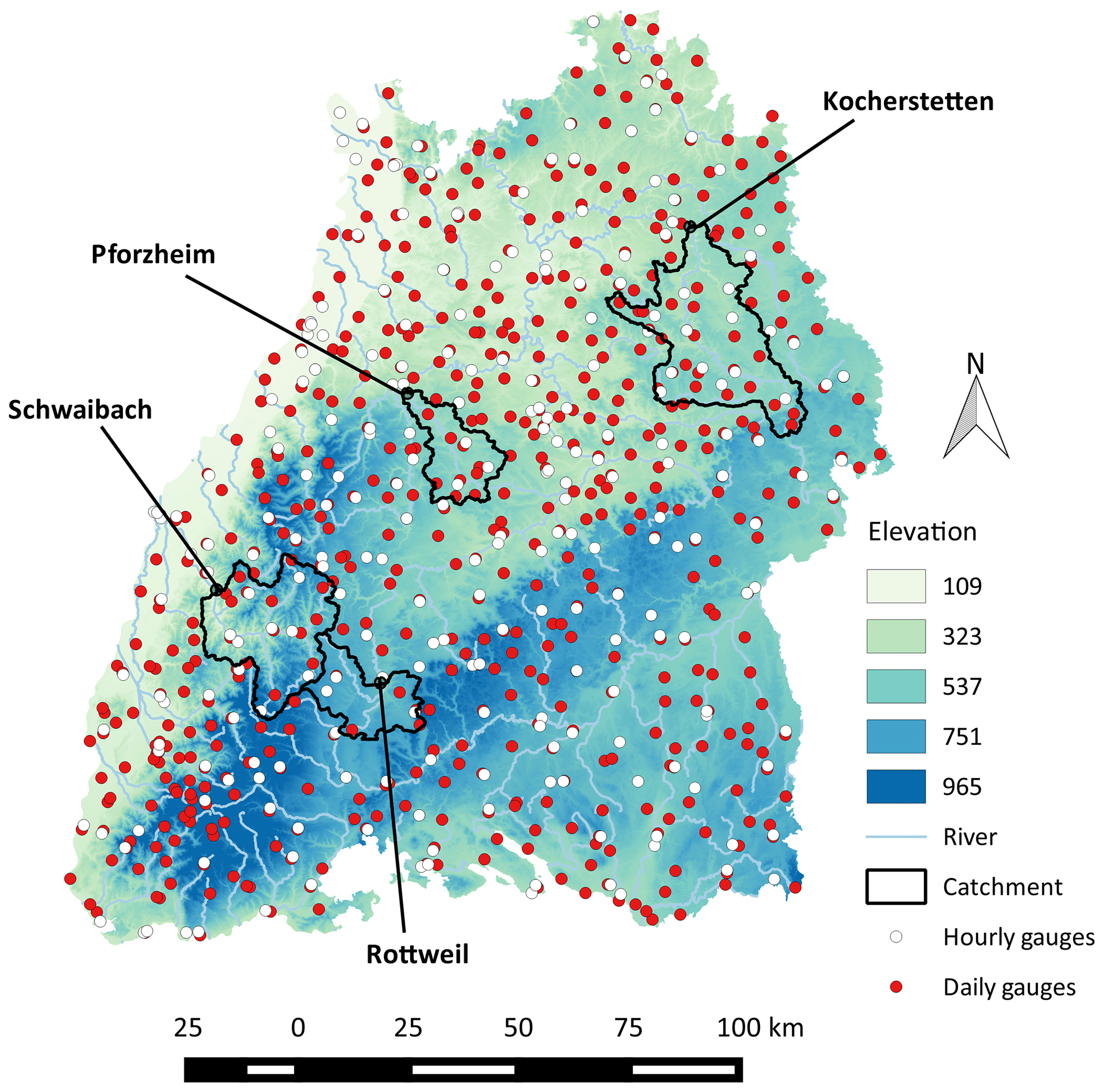
Figure 1 Locations of the sub-daily and daily rain gauges in Baden-Württemberg and the four selected catchments.

Rainfall data from a dense network of daily rainfall stations (62 km² per station in 1991) and from a less dense network of sub-daily stations (144 km² per station in 1991) with high-resolution rainfall observations were used for this study. All data are available for the time period 1991–2010. The number of available daily stations and sub-daily stations varies according to different time periods. Figure 2 illustrates the number of available observation stations in Baden-Württemberg between 1991 and 2010. It can be seen from the graph that more than 430 daily stations but only 30 sub-daily stations were available in 1991. The total number of daily stations decreased to 250 around 2003 and remained stable for the subsequent years. The number of sub-daily stations has been increasing throughout this period and experienced a sharp increase from 100 to 200 in 2005. Four different rainfall datasets were generated and explained as follows.

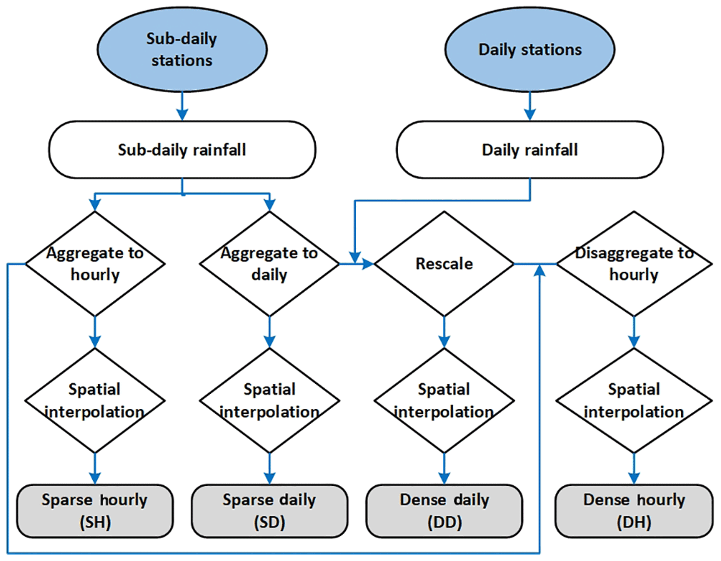
1. High temporal resolution observed rainfall was aggregated to hourly and then interpolated to 1×1 km² grids using the ordinary kriging algorithm (Matheron, 1963). The correlation function obtained from the cross-correlations of the hourly time series was used as a basis for the variogram. This set is referred to as the Sparse Hourly (SH) set.

2. Observed daily rainfall combined with the daily aggregations of the high temporal resolution data were used to create 1×1 km² gridded datasets using the ordinary kriging algorithm. The variogram was based on the cross-correlations of the daily time series. This set is referred to as the Dense Daily (DD) set.

3. High-resolution rainfall was aggregated to daily time steps and interpolated subsequently for a 1×1 km² grid using the ordinary kriging. The variogram was based on the cross-correlations of the aggregated daily time series. This set will be referred to as the Sparse Daily (SD) set.

4. Observed daily rainfall combined with the hourly aggregations of the high temporal resolution data were used to create a 1×1 km² grid using the disaggregation method rescaled ordinary kriging (Bárdossy and Pegram, 2016b). The variogram was based on the cross-correlations of the hourly time series. This set is referred to as the Dense Hourly (DH) set.

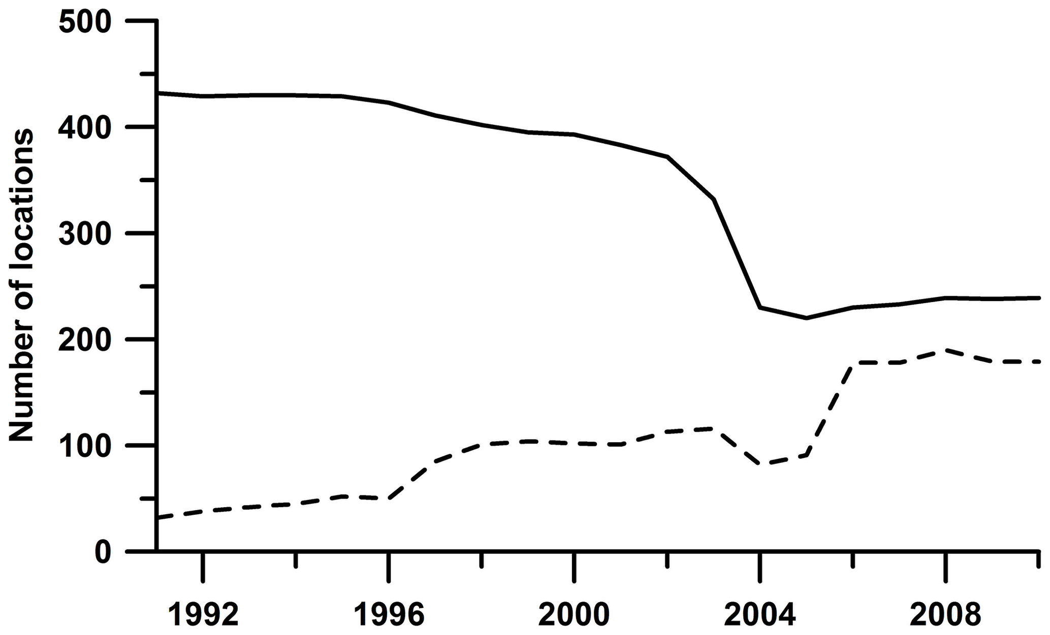
Figure 2 The number of available observation locations. Daily stations – solid line; sub-daily stations – dashed line.

Figure 3 shows the flowchart of the data collection and process. The DD and SD sets are the daily aggregations of the DH and SH sets. Note that DH is a dataset combining hourly and disaggregated daily gauge data. One of the research questions raised here is to find out whether disaggregation leads to an improvement in model performance. Comparisons of the model performance using the inputs of the (SD, SH) and (DD, DH) pair will reveal the effect of temporal resolution. Meanwhile, comparison between (SD, DD) and (SH, DH) will show the influence of the rainfall observation network density on the model performance.

Figure 3 Schematic representation of four different rainfall datasets.

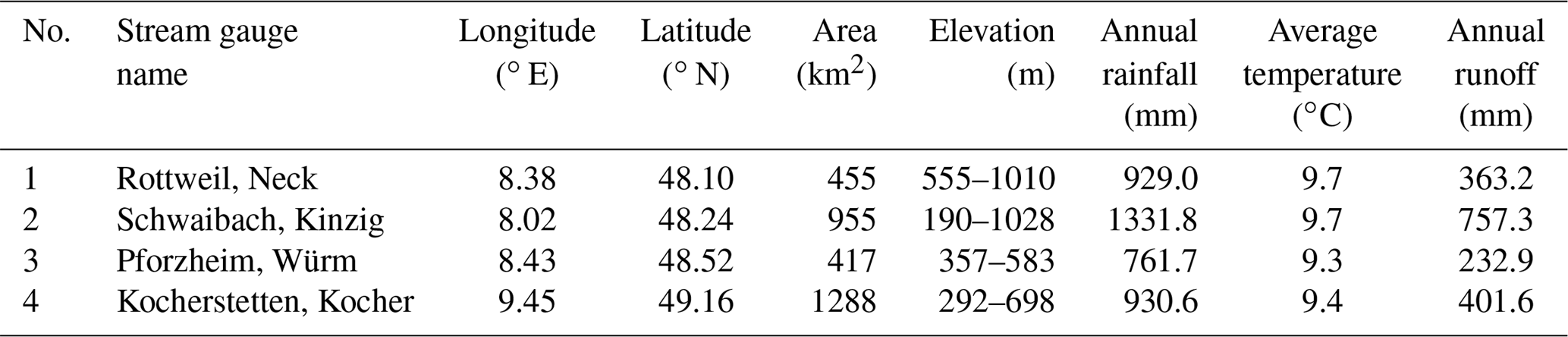
Four mesoscale catchments (Fig. 1), namely Rottweil, Schwaibach, Pforzheim and Kocherstetten, were selected from the upstream region of the state for testing the sensitivity of model performance to the four different rainfall datasets. The daily streamflow record of these catchments was collected for the period 1991–2010. The basic characteristics for the study catchments are listed in Table 1. These catchments range in size from 417 to 1300 km², along with large differences in elevation and annual precipitation. It can be seen clearly from the map that these four catchments have different raingauge densities; the Schwaibach catchment located in the mountainous area with elevations ranging from 190 to 1028 m has the lowest density of raingauge networks and the highest annual precipitation. Rottweil and Kocherstetten have similar climate conditions in terms of annual precipitation and runoff, but the catchment size of Kocherstetten is almost 3 times that of Rottweil. Pforzheim has the smallest drainage area and the lowest amount of precipitation.

Table 1 Catchment characteristics for the four selected catchments.

3 Model and methodology

3.1 Model structure

The conceptual HBV model was developed in the 1970s by the Swedish Meteorological and Hydrological Institute (SMHI) (Bergström and Forsman, 1973). Thanks to its simplicity, low demand of inputs and small number of model parameters, the HBV model has been widely used for rainfall–runoff simulation and flood forecasting. Figure 4 represents the structure diagram of the HBV model (Singh, 2010). There are three main modules in the HBV model, namely snow routine, soil moisture routine and runoff routine (Hartmann, 2007; Singh, 2010).

Figure 4 Schematic representation of the HBV model.

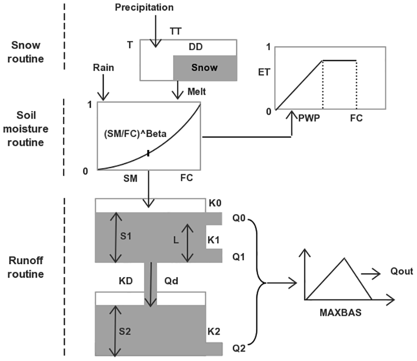
In the snow routine, the snow accumulation and melting process is estimated by the relatively simple degree-day method (Rango and Martinec, 1995) with two parameters: degree-day factor (DD) and threshold temperature for snow/rain (TT) (as shown in Eq. 1). The measured precipitation is supposed to be solid (snowfall) if the air temperature is lower than threshold temperature; otherwise, precipitation appears in a liquid state (rainfall) if the weather is warmer than the threshold value.

$$\begin{array}{}\text{(1)}& \mathrm{Snowmelt}=\mathrm{DD}\cdot (T-\mathrm{TT}),\mathrm{if}T>\mathrm{TT}\end{array}$$

In the HBV model, soil moisture storage is decided by balancing rainfall and evapotranspiration according to two soil moisture constants: permanent wilting point (PWP) and field capacity (FC). The soil wetness index, defined as the ratio of direct runoff to effective precipitation ($\frac{\mathrm{\Delta }Q}{\mathrm{\Delta }P}$), is expressed as

$$\begin{array}{}\text{(2)}& {\displaystyle \frac{\mathrm{\Delta }Q}{\mathrm{\Delta }P}}={\left({\displaystyle \frac{\mathrm{SM}}{\mathrm{FC}}}\right)}^{\mathrm{Beta}},\end{array}$$

where SM denotes the actual soil moisture and “Beta” the proportion of effective precipitation contributing to runoff for given soil moisture. The Penman equation is used to estimate the potential evapotranspiration according to the long-term monthly mean air temperature (T_M) and long-term monthly averaged potential evapotranspiration (PE_M) (Penman, 1948):

$$\begin{array}{}\text{(3)}& E_{\mathrm{tp}}=\left(\mathrm{1}+C\left(T-T_{\mathrm{M}}\right)\right){\mathrm{PE}}_{\mathrm{M}},\end{array}$$

where C is the evapotranspiration coefficient. The actual evapotranspiration (E_ta) can be estimated as

$$\begin{array}{}\text{(4)}& E_{\mathrm{ta}}=\left\{\begin{array}{ll}{E}_{\mathrm{tp}}& \mathrm{if}\mathrm{SM}>\mathrm{PWP}\\ \frac{\mathrm{SM}}{\mathrm{PWP}}\cdot E_{\mathrm{tp}}& \mathrm{else}\end{array}\right..\end{array}$$

As shown in Eq. (2), runoff is calculated by a nonlinear function based on excessive effective precipitation and actual soil moisture. The runoff concentration process consists of upper and lower reservoirs with five parameters:

$$\begin{array}{}\text{(5)}& {\displaystyle }& {\displaystyle }{Q}_{\mathrm{0}}=K_{\mathrm{0}}\left(S_{\mathrm{1}}-\mathrm{HL}\right),\text{(6)}& {\displaystyle }& {\displaystyle }{Q}_{\mathrm{1}}=K_{\mathrm{1}}{S}_{\mathrm{1}},\text{(7)}& {\displaystyle }& {\displaystyle }{Q}_d=K_d{S}_{\mathrm{1}},\text{(8)}& {\displaystyle }& {\displaystyle }{Q}_{\mathrm{2}}=K_{\mathrm{2}}{S}_{\mathrm{2}}.\end{array}$$

The runoff is divided into surface flow (Q₀), interflow (Q₁) and baseflow (Q₂) with three recession coefficients K₀, K₁ and K₂, along with a conceptual threshold water level (HL) for generating surface flow. The two parallel reservoirs are connected in the form of percolation storage (Q_d) from the upper reservoir to the lower one with the parameter of the percolation constant K_d. A transformation function with the triangular weighting parameter MAXBAS is used to smooth the total runoff ($Q_{\mathrm{0}}+Q_{\mathrm{1}}+Q_{\mathrm{2}}$) to obtain discharge at the outlet.

In this study, to investigate the sensitivity of model performance to the spatial resolution of input variables, two HBV models with different spatial configurations were applied: lumped HBV and spatially distributed HBV, respectively. In the lumped model, precipitation, temperature and potential evapotranspiration were assumed uniformly distributed within a catchment and all the processes were calculated for the whole catchment. Previous studies have indicated that the elevation is an important reason for the spatial differentiation of meteorological variables, including temperature, precipitation, evapotranspiration and snowmelt, being in reality not uniformly distributed within a catchment. They often exhibit dependence with elevation. The spatially distributed HBV model used in this study divides a catchment into several zones based on elevation. The 1×1 km² grid-based rainfall and temperature data were averaged for each elevation zone. In the spatially distributed model, the parameters associated with the snowmelt and soil moisture modules were calibrated for each elevation zone. The parameters associated with the runoff response module were calibrated for each catchment similarly to the lumped model (Das et al., 2008).

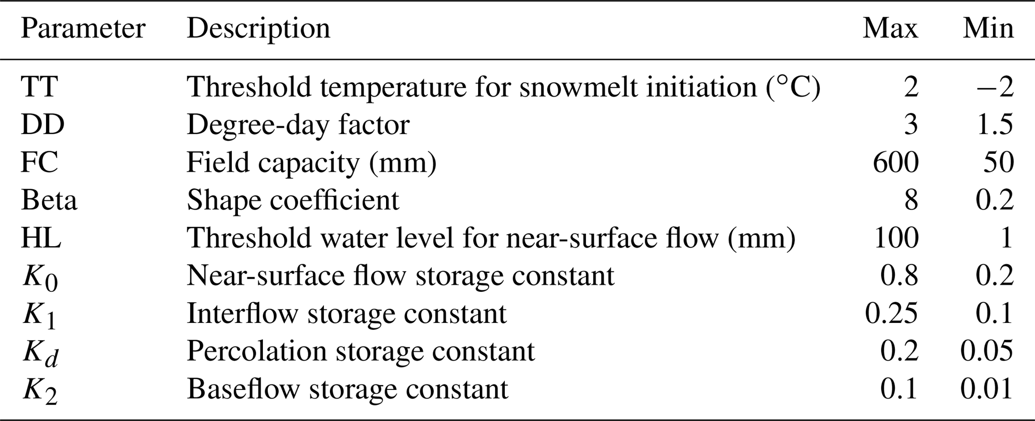
Out of the 15 parameters within the HBV model, 9 parameters were calibrated in this study. Table 2 lists the initial upper and lower limits of the to-be-calibrated parameters using historical data. The data-depth-based parameter optimization method – the Robust Parameter Estimation (ROPE) algorithm (Bárdossy and Singh, 2008) – was applied for model parameter optimization. The ROPE approach could lead to a certain number of model parameters with ideal model performance (Bárdossy et al., 2016). For this study, each simulation results in 10 000 heterogeneous parameter sets with similarly acceptable model performance.

Table 2 Description of HBV model parameters and parameter ranges for model calibration.

3.2 Performance criteria

Previous studies have shown that model performance strongly depends on the selection of performance criteria (Gupta et al., 2009). The model simulations corresponding to the model parameters using different objective functions differ considerably as they have different focuses (Bárdossy et al., 2016). The purpose of this study is to investigate the sensitivity of the conceptual model to rainfall variability and accordingly find effective ways to improve the precision of flood forecasting. Since high flow is extremely important for flood forecasting, the Nash–Sutcliffe (NS) coefficient (Nash and Sutcliffe, 1970), one of the widely used indicators, was used in this study to assess the model performance based on observed discharge. The NS coefficient focuses on high flow as it evaluates the squared difference between simulated and measured streamflow. It can be calculated using the following equation:

$$\begin{array}{}\text{(9)}& \mathrm{NS}=\mathrm{1}-{\displaystyle \frac{\sum _{t=\mathrm{1}}^T{\left(Q_{\mathrm{o}}\left(t\right)-Q_{\mathrm{m}}\left(t\right)\right)}^{\mathrm{2}}}{\sum _{t=\mathrm{1}}^T{\left(Q_{\mathrm{o}}\left(t\right)-\stackrel{\mathrm{‾}}{Q_{\mathrm{o}}}\right)}^{\mathrm{2}}}},\end{array}$$

where Q_o(t) and Q_m(t) are the observed and simulated discharge, respectively, and $\stackrel{\mathrm{‾}}{Q_{\mathrm{o}}}$ is the mean of the observed discharge.

The mean square error (MSE) of the flow for the time period of the observed discharge higher than the 10th percentile of flow was used to assess the flood forecasting ability of the models:

$$\begin{array}{}\text{(10)}& \mathrm{MSE}={\displaystyle \frac{\mathrm{1}}{n}}\sum _{i=\mathrm{1}}^n{\left(Q_{\mathrm{o}}\left(i\right)-Q_{\mathrm{m}}\left(i\right)\right)}^{\mathrm{2}},\end{array}$$

where Q_o(i) and Q_m(i) are the observed and modeled discharges when the observed discharge is higher than the 10th percentile of flow.

3.3 Model calibration experiments

A split-sample calibration methodology was applied in this study to divide the data into two 10-year periods: 1991–2000 and 2001–2010. Model calibration was carried out for both time periods and then a cross-validation analysis was performed. For each calibration run, the first water year data were used as a warm-up period and were not used to evaluate the model performance.

In this study we investigated the impacts of using different methods for spatial interpolation of hourly rainfall data on model performance. The four rainfall datasets were used as input variables for model calibration and validation. In all modeling experiments, daily mean temperature and potential evapotranspiration were used as inputs. This is to isolate the effects of different rainfall inputs on the model performance. The effects of the temporal and spatial resolutions of the rainfall inputs on the model performance were assessed in terms of the NS coefficient and the MSE of the high flow. We conducted experiments of model calibration for a lumped model and a spatially distributed HBV model using hourly and daily input variables, respectively. For the spatially distributed model structure, a contour interval of 100 m was used to divide a catchment into different elevation zones. Note that all the model calibrations were performed on the basis of simulating daily discharge.

We investigated whether the combination of daily and hourly models can lead to better prediction in streamflow. It is interesting to investigate the similarities of different temporal resolution. Therefore, the common calibration approach was used to calibrate the daily and hourly models simultaneously. This approach may identify robust model parameters that are applicable using different temporal resolutions. The common calibration approach is a multi-objective optimization function, and the compromise programming method (Zeleny, 1981) was used to formulate the objective function:

$$\begin{array}{}\text{(11)}& O\left(\mathit{\theta }\right)=\sum _{i=\mathrm{1}}^n{\left({\mathrm{NS}}_{\mathrm{i}}^{*}-{\mathrm{NS}}_{\mathrm{i}}\left(\mathit{\theta }\right)\right)}^p.\end{array}$$

Here index i denotes the type of temporal resolution; NS${}_{\mathrm{i}}^{*}$ means the optimal model performance which can be represented by the individual calibrated model performance. Here we aim to minimize the value of the objective function O(θ). For the balancing factor p, a moderately high p=4 was given in this study. More details about the common calibration of hydrological models' strategy can be found in Bárdossy et al. (2016).

4 Results and discussion

4.1 Comparison of the rainfall datasets

The quality of the rainfall datasets was assessed and compared for the four selected catchments. As the SD and DD sets are daily aggregations of the SH and DH sets, we only compared daily rainfall sets SD and DD for both calibration periods (Fig. 5). It can be seen clearly from the figures that the interpolated rainfall datasets display some differences for all study catchments. The asymmetry of the scatterplots is evident for the period 1991–2000. In general, the DD dataset leads to higher values than the SD dataset. This is mainly because the low density of sub-daily observations during the period of 1991–2000 leads to large errors in the spatial interpolation of rainfall. This is especially the case for Schwaibach catchment, which varies strongly in geographical elevation (from 190 to 1028 m). For the period of 2001–2010, the SD and DD sets are in closer agreement due to the higher density of sub-daily gauges.

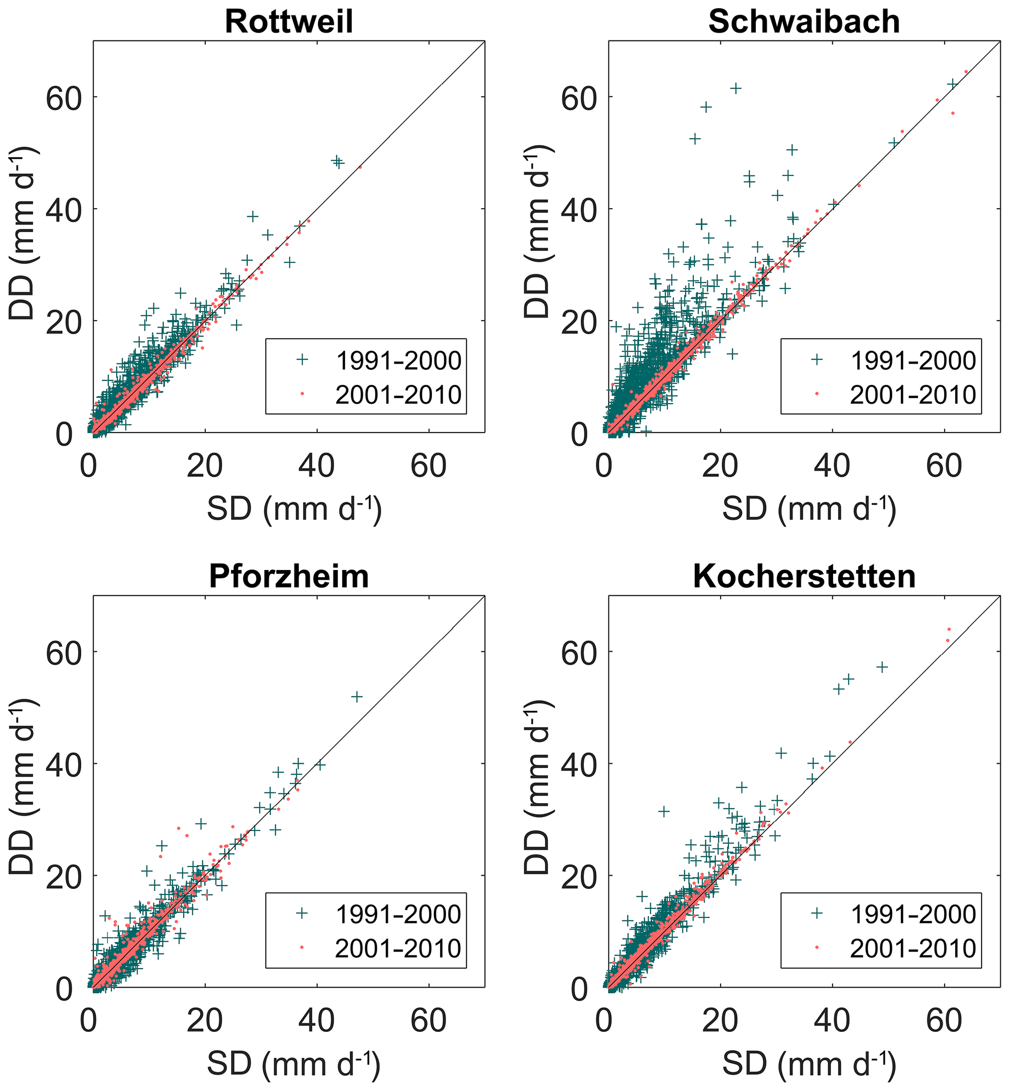
Figure 5 Comparison of the daily rainfall data that were interpolated using different densities of raingauge networks.

4.2 Results of calibration and validation

As described in Sect. 3.3, for the selected catchments, model calibrations were carried out using four rainfall datasets for both lumped and spatially distributed HBV models. Two 10-year time periods, 1991–2000 and 2001–2010, were used for calibration and cross-validation. In total 16 calibration runs and 16 validation runs were performed for each catchment. As mentioned before, each simulation obtained 10 000 parameter sets with similar model performance. We then used the mean value of the 10 000 model performances to quantify the model performance.

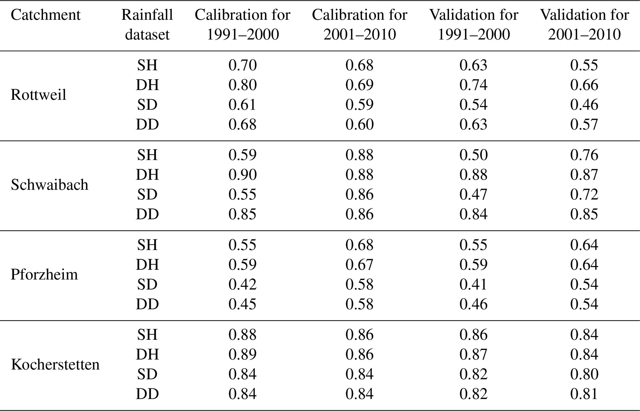
Table 3 lists the average value of the NS model performance for the four selected catchments using the lumped HBV model and Table 4 lists the simulated NS performance for a spatially distributed version of the model, respectively. The results show that all four datasets can reproduce relatively accurate historical daily streamflow series for all selected catchments. Results also show that the model performances vary across catchments. The Kocherstetten catchment generally performs best, with an average NS value of 0.84 for all simulations, while Pforzheim has the worst mean NS performance of 0.58 for all calibration runs. Moreover, for a specific catchment, the calibrated models perform differently for different data periods. For the Schwaibach and Pforzheim catchments, the calibrated model performance for the period of 2001–2010 is better than the performance for the time period 1991–2000 for most of the datasets. This might be due to the increasing raingauge density inside or near the catchment and the quality of rainfall data with the development of time and technological progress. In particular, the model calibrations for the period 1991–2000 of the Schwaibach catchment using sets SH and SD perform very poorly for both calibration and validation. The NS coefficient using SH and SH inputs is about 0.3 less than the results of sets DH and DD. This indicates that systematic interpolated rainfall errors have a critical influence on model calibration.

Table 3 Average NS model performance for the lumped HBV model.

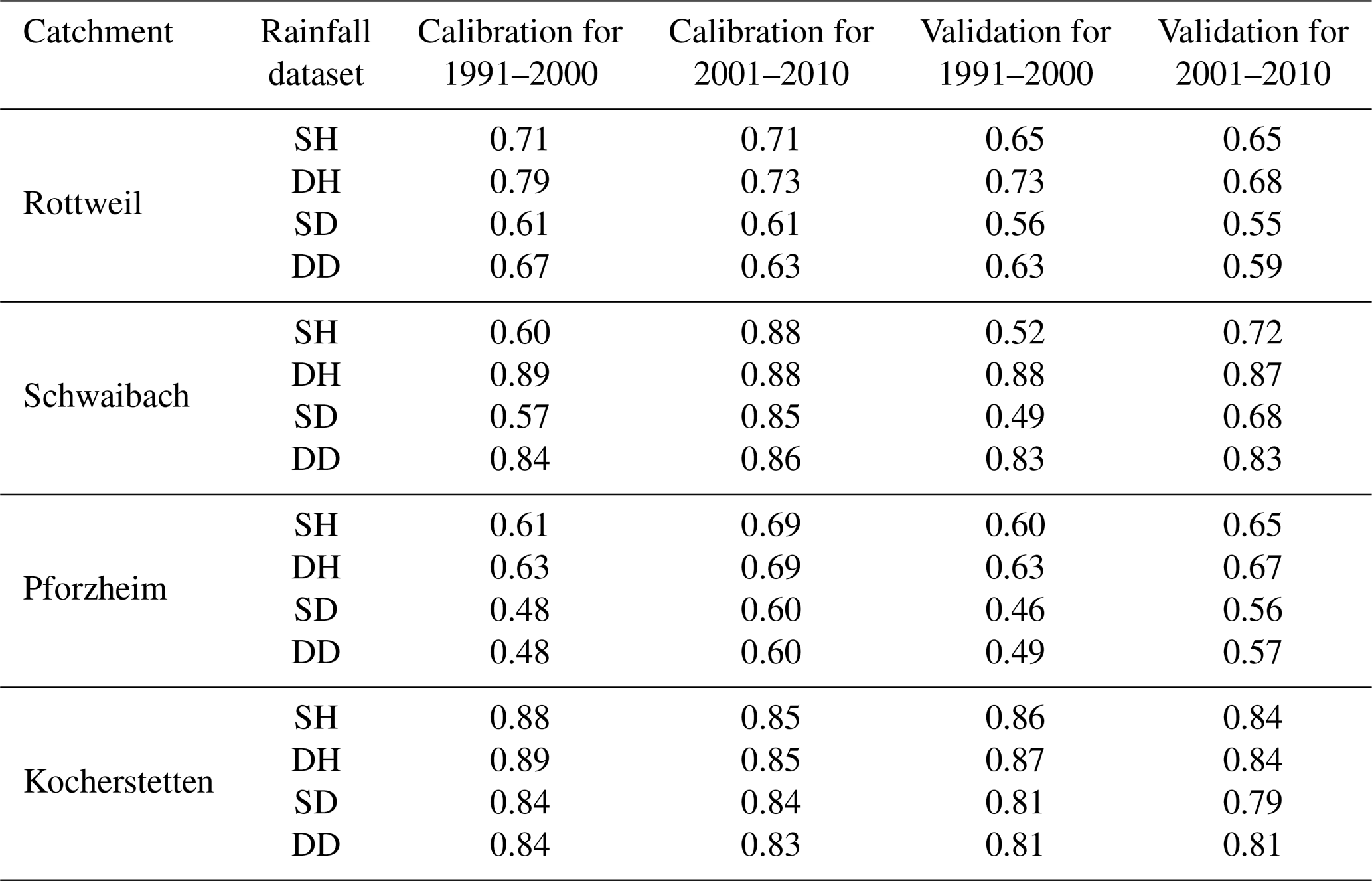
Table 4 Average NS model performance for the distributed HBV model.

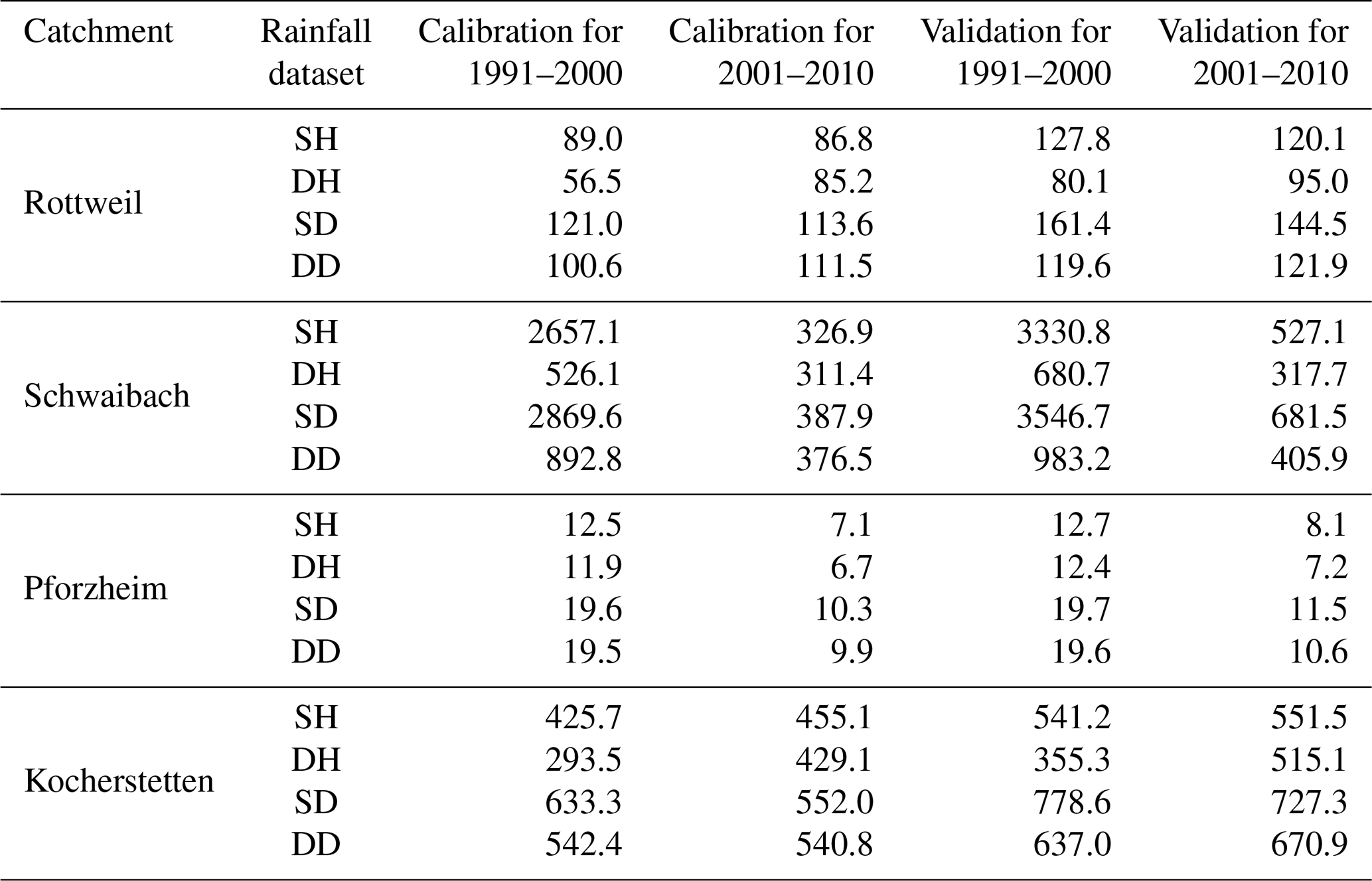
We then analyzed whether the model is robust for simulating high flows. Tables 5 and 6 list the mean square errors of the top 10th percentile of flows for the lumped and spatially distributed models, respectively. Figure 6 shows the flow duration curve for the natural logarithm of simulated and observed discharge for all study catchments for the years between 2001 and 2010. Figure 7 shows the corresponding results for flows higher than the 10th percentile of flow. Results indicate that for most of the calibration runs, set DH performs best for the high flow, followed by set SH, set DD performs a little weaker than set SH, while set SD has the worst performance in flood simulation.

Figure 6 Comparison of the simulated flow duration curve.

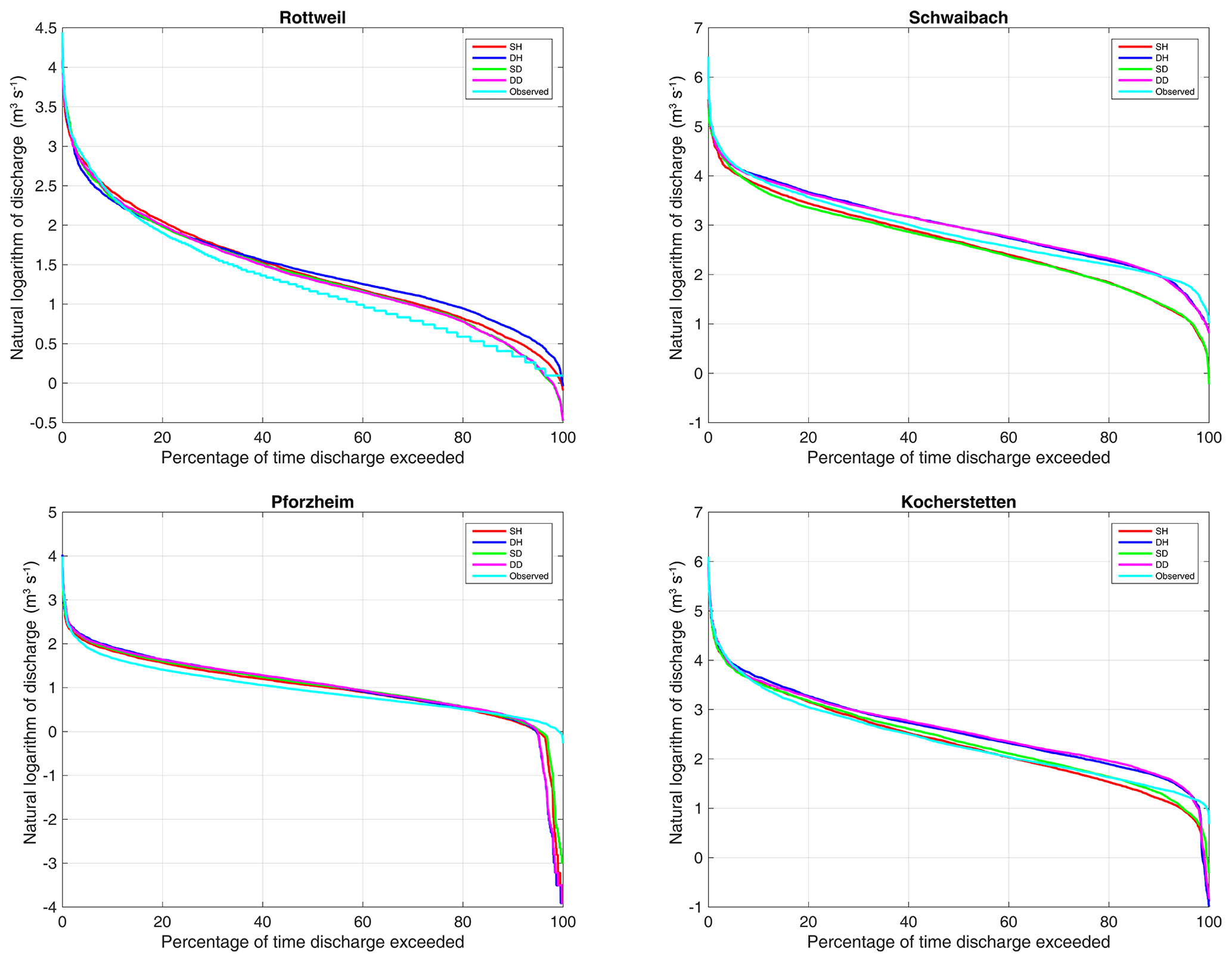
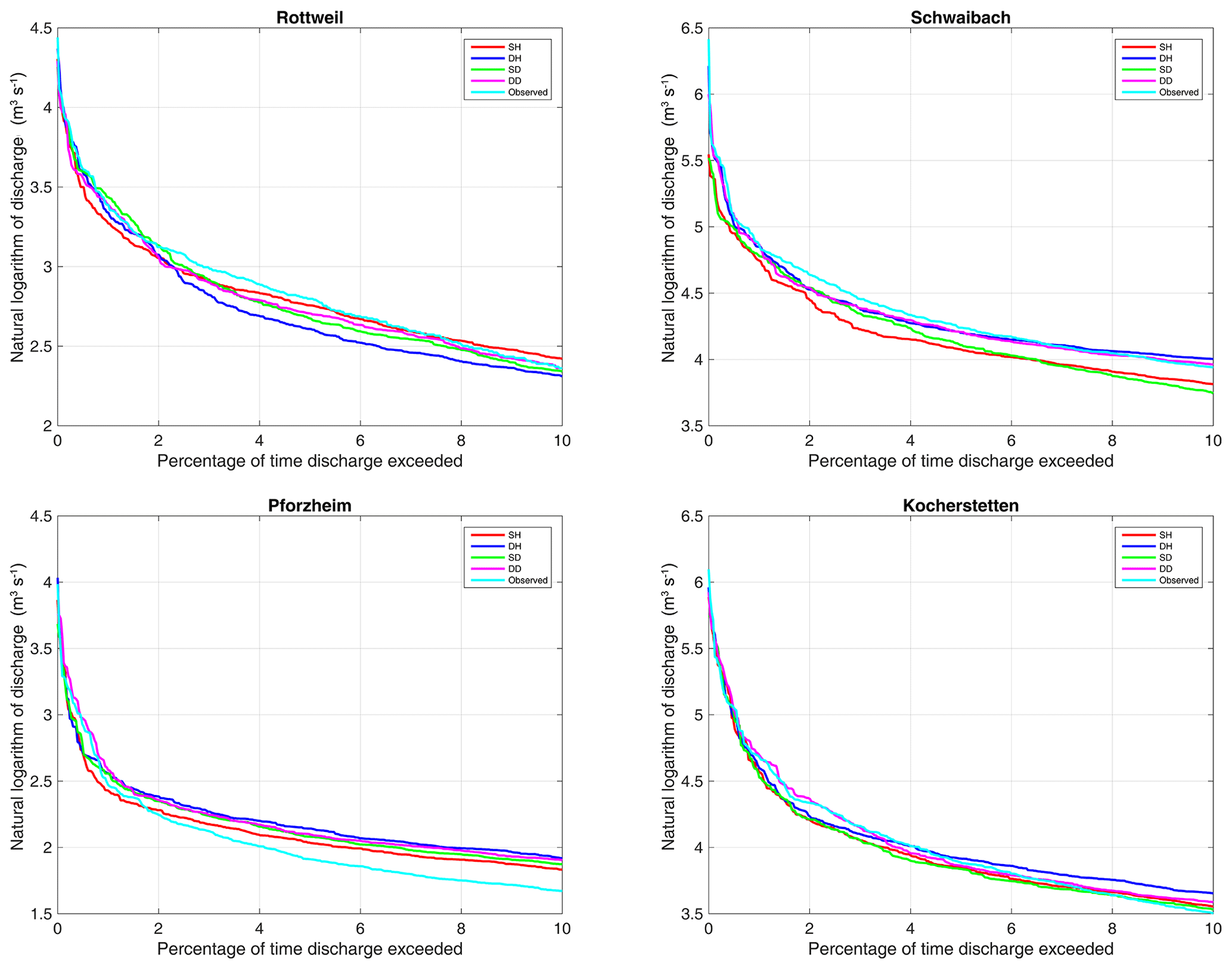
Figure 7 Comparison of the simulated flow duration curve for flows higher than the 10th percentile of flow.

Table 5 Mean square error for flows higher than the 10th percentile of flow for the lumped HBV model.

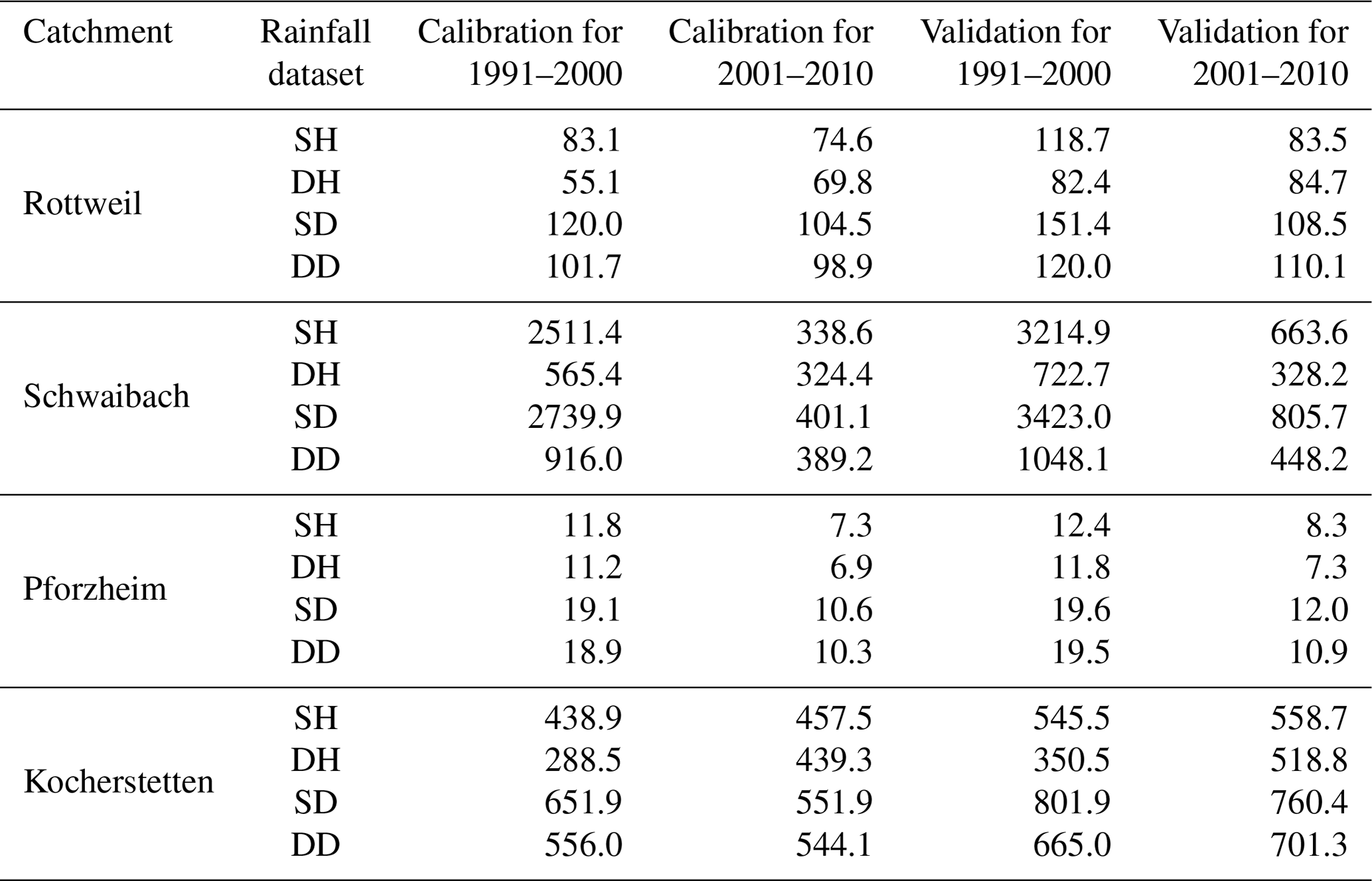
Table 6 Mean square error for flows higher than the 10th percentile of flow for the distributed HBV model.

4.3 Model performance using different temporal resolutions of rainfall data

Firstly, the model performance of different temporal resolutions of rainfall was compared for four datasets and two model spatial configurations. For the pairwise comparison, all the conditions are the same in the model except for the rainfall temporal resolution (hourly and daily). The results of the sparse sets and dense sets are separated here. Figure 8 compares the model performance of using hourly and daily rainfall inputs that were interpolated using only high-resolution rainfall observations (SH, SD). Figure 9 compares the results from the rainfall inputs that incorporated observed daily values with high-resolution observations (DH, DD). The result shows that all the scatters are lying below the diagonal line for the different levels of observation density. For both the calibration and validation periods, the simulations using hourly input data outperform the ones based on the daily resolution. For the dataset with low observation network density, the averaged NS of set SH is about 0.73 for the calibration period and 0.68 for the validation period, while the mean NS coefficient calibrated using the SD set is 0.67 and 0.6, respectively. The higher observation density datasets show a similar tendency. The mean NS of using the DH set is around 0.79 for calibration and 0.77 for validation, while that of set DD is 0.72 and 0.69, respectively. The fact that the hourly scale model performs better than the daily model suggests that the dynamic runoff of the catchment could be better simulated with a higher temporal resolution of rainfall. According to the distances from the diagonal to the scatterplots, we can observe that the difference in model performance for different temporal resolutions is larger for the catchments with relatively low NS model performance, such as Schwaibach and Pforzheim. For Rottweil and Kocherstetten, the performance of the hourly calibrated model is only slightly better than the daily model.

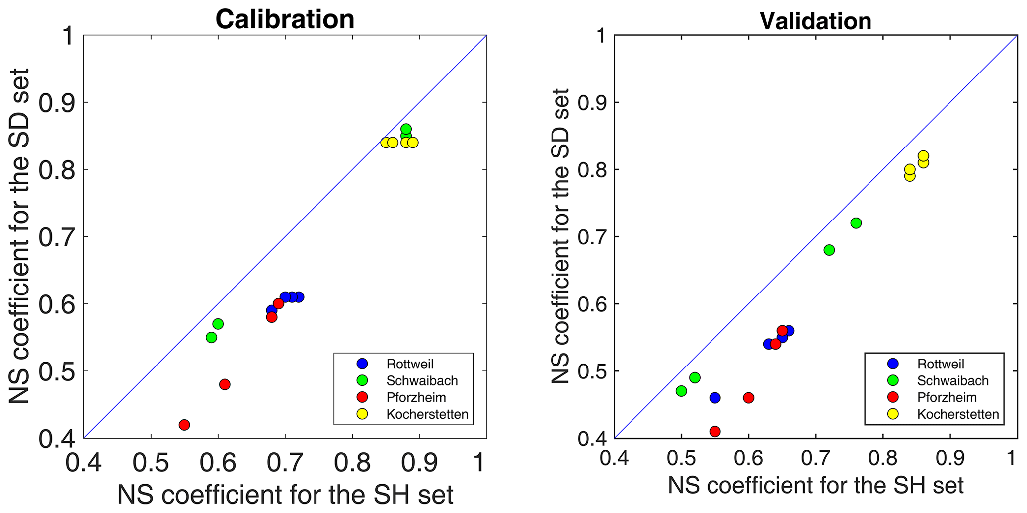
Figure 8 Comparison of the NS coefficient for using hourly and daily rainfall as model input for the SH and SD sets.

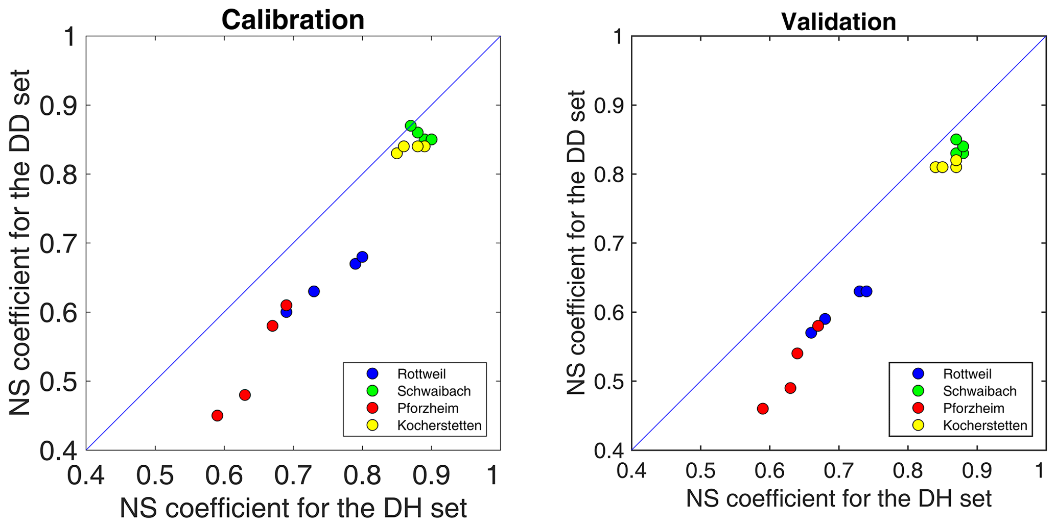
Figure 9 Comparison of the NS coefficient for using hourly and daily rainfall as model input for the DH and DD sets.

4.4  Model performance in terms of observation density

The rainfall gauge network density has a significant impact on model simulation and parameter optimization. Figure 10 shows the simulated NS coefficient of the model simulations using the daily input data interpolated using different densities of raingauge networks. It shows obviously from the location of points that the simulated model performance using the DD set is generally better than that using the SD set for both the calibration and validation periods. The averaged NS model performances of DD and SD sets are 0.71 and 0.64, respectively. The model performance using hourly inputs shows a similar trend to that using daily inputs. As shown in Fig. 11, the model using the DH set outperforms the one using the SH set. These results demonstrate that high raingauge density led to improvement in model performance at both daily and hourly time resolution.

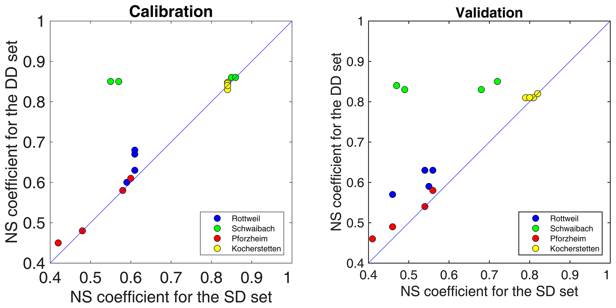
Figure 10 Comparison of the NS coefficient for different densities of raingauge networks; models were simulated based on daily time steps.

Figure 11 Comparison of the NS coefficient for different densities of raingauge networks; models were simulated based on hourly time steps.

Figure 12 illustrates the cumulative distribution function of the NS coefficient using sets SD, SH and DH for model calibration (left) and validation (right). As can be seen clearly from the curves, if rainfall data come from a sparse network of sub-daily stations, use of higher temporal resolution datasets (the SH set) leads to better model performance than using lower-resolution ones (the SD set). Simulation of daily streamflow can benefit from running the model at a higher temporal resolution. In addition, the combination of observed sub-daily rainfall with disaggregated daily rainfall (the DH set) leads to a further improvement in daily streamflow simulation.

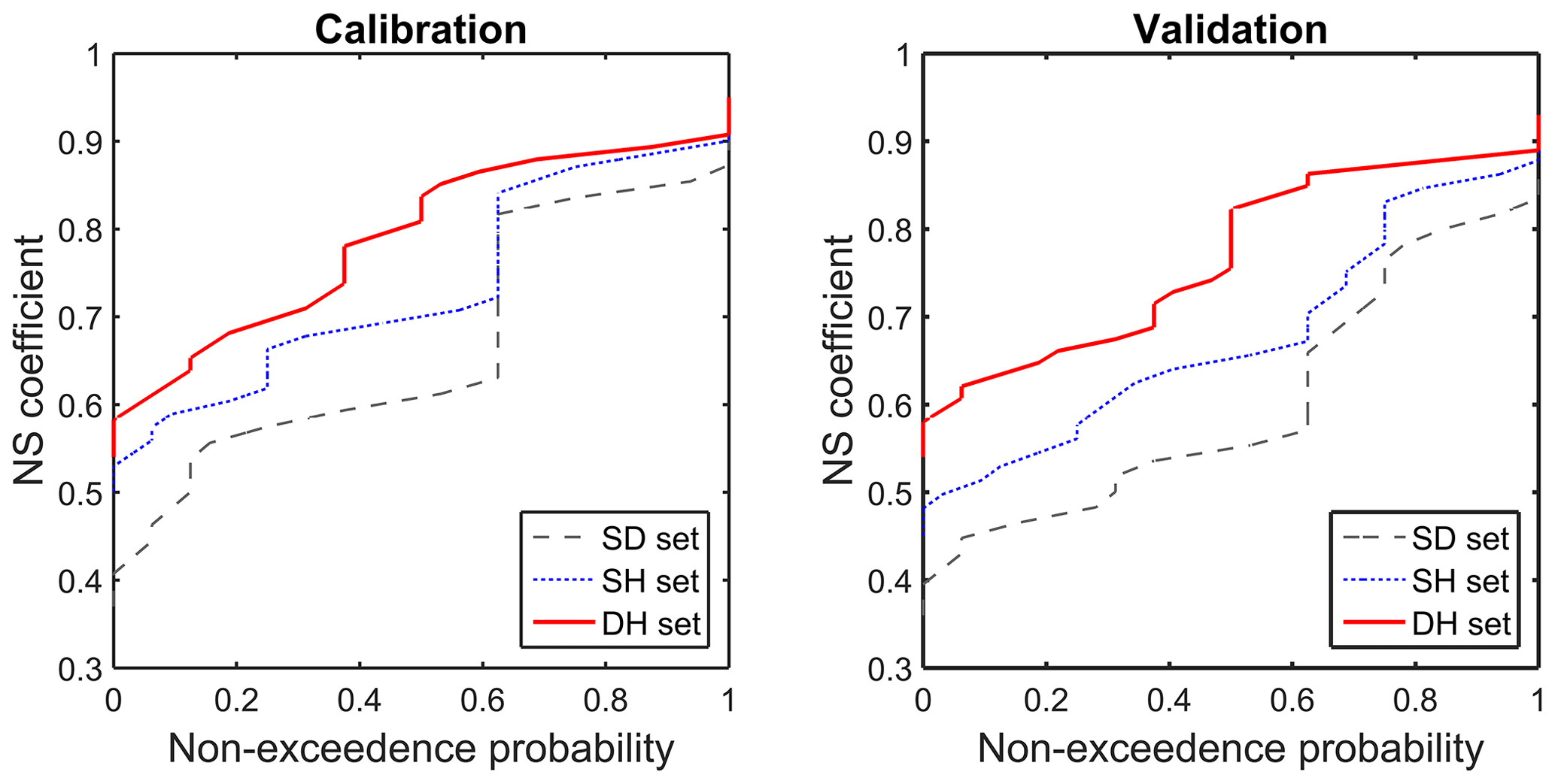
Figure 12 Cumulative distribution of the NS coefficient for model calibration using different rainfall datasets.

4.5 Model performance in terms of the spatial resolution of rainfall data

The model performance was compared between the lumped and spatially distributed HBV models when they were driven by different rainfall datasets. Figure 13 compares the NS model performance for calibration (left) and validation (right) periods. The correlation between model performance and the spatial resolution of a model seems unclear for the study catchments. For some simulations, the spatially distributed model outperforms the lumped one, especially for the catchments with a high NS coefficient, despite the increase in model performance being only marginal. However, for the catchments with relatively poorer model performance, the lumped model could even lead to slightly better performance than the semi-distributed model, especially for the validation period when the difference seems larger than the calibration period. This indicates that for model validation, the model parameters estimated by the distributed HBV model show weaker transferability. A possible explanation for this case could be that the distributed model has a larger number of parameters to be calibrated and that the parameters are underestimated during the calibration period. We conclude that the improvement in the spatial resolution of model structure did not enhance the model performance, which is surprising since higher spatial resolution and more model parameters are expected to improve the model performance. Our results confirm the findings of Das et al. (2008) that the distributed models do not necessarily improve model performance.

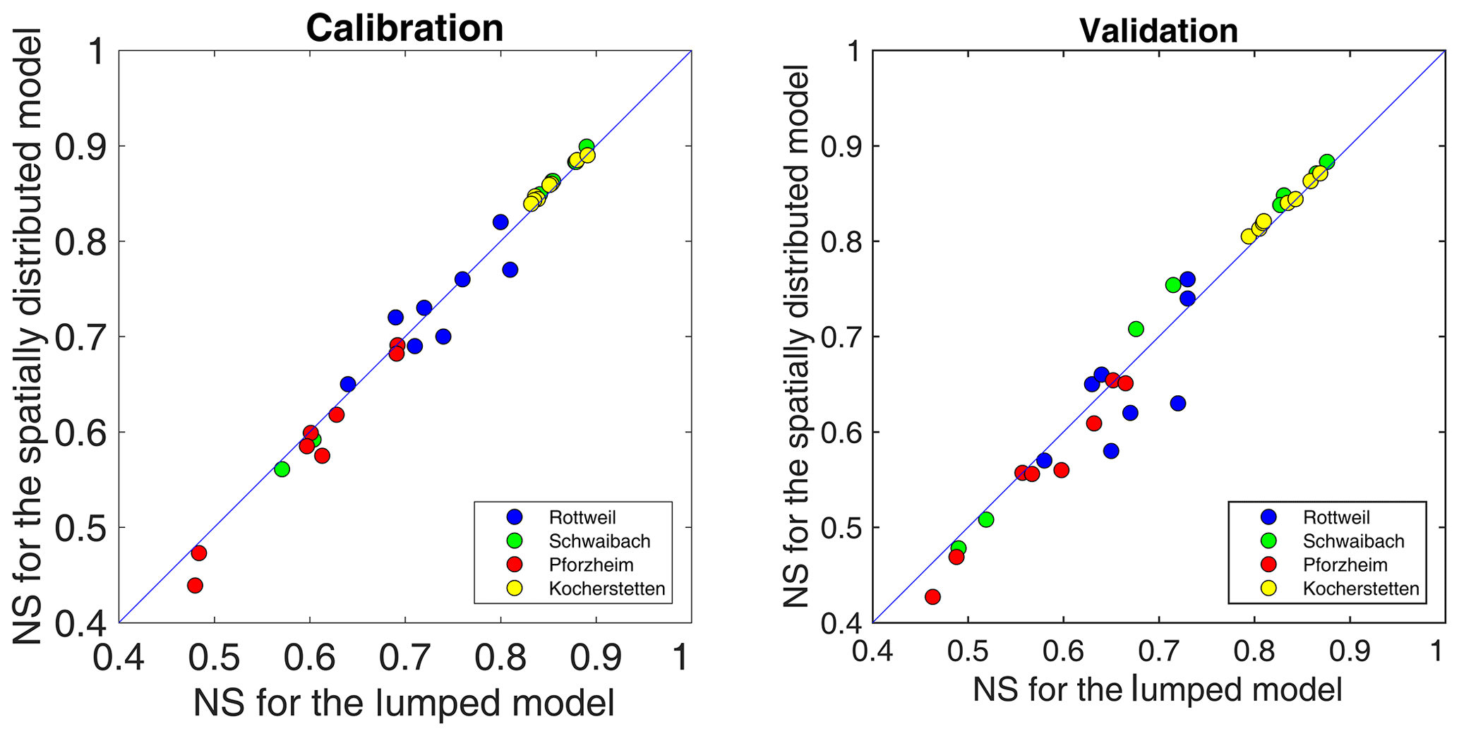
Figure 13 Comparison of the NS coefficient for different spatial resolutions of model structure.

The distributed model did not perform better than the lumped model in this study. This could be because the catchment underlying surface information and/or the calibration procedure was not sufficient for identifying optimal distributed model parameters. A second reason could be that the temporal resolution of the rainfall inputs is not sufficient for the distributed model.

4.6 Common model calibration with different temporal resolutions

As shown before, the combination of hourly and daily gauge data leads to the improvement in data quality as the model using sets DH and DD has better performance than using sets SH and SD. Furthermore, common calibration of the lumped HBV model was performed for sets DH and DD to identify model parameters good for both hourly and daily time steps. It is important to note that the parameters (DD, K₀, K₁, K_d and K₂) that are dependent on time steps should be converted according to the simulation step of the model. The common calibration was performed for the two time periods separately, and a cross-validation analysis was performed as well. The common calibration and validation results were compared with the individual calibration (Fig. 14). For the calibration period, the common calibration always leads to slightly weaker performance for all datasets. For three of the DD datasets, model performances of common parameters are similar to individual calibration results. The average loss of NS coefficients over all catchments is about 0.02 for set DH and 0.01 for set DD. For the validation period, it can be seen from the scatterplots that the common parameters outperform the individual ones for about half of all the simulations. It suggests that parameter values obtained using the common calibration approach based on different time steps can improve the temporal transferability of models. The reason for the robustness of common parameters might be that a common calibration strategy can provide more information for identifying model parameters.

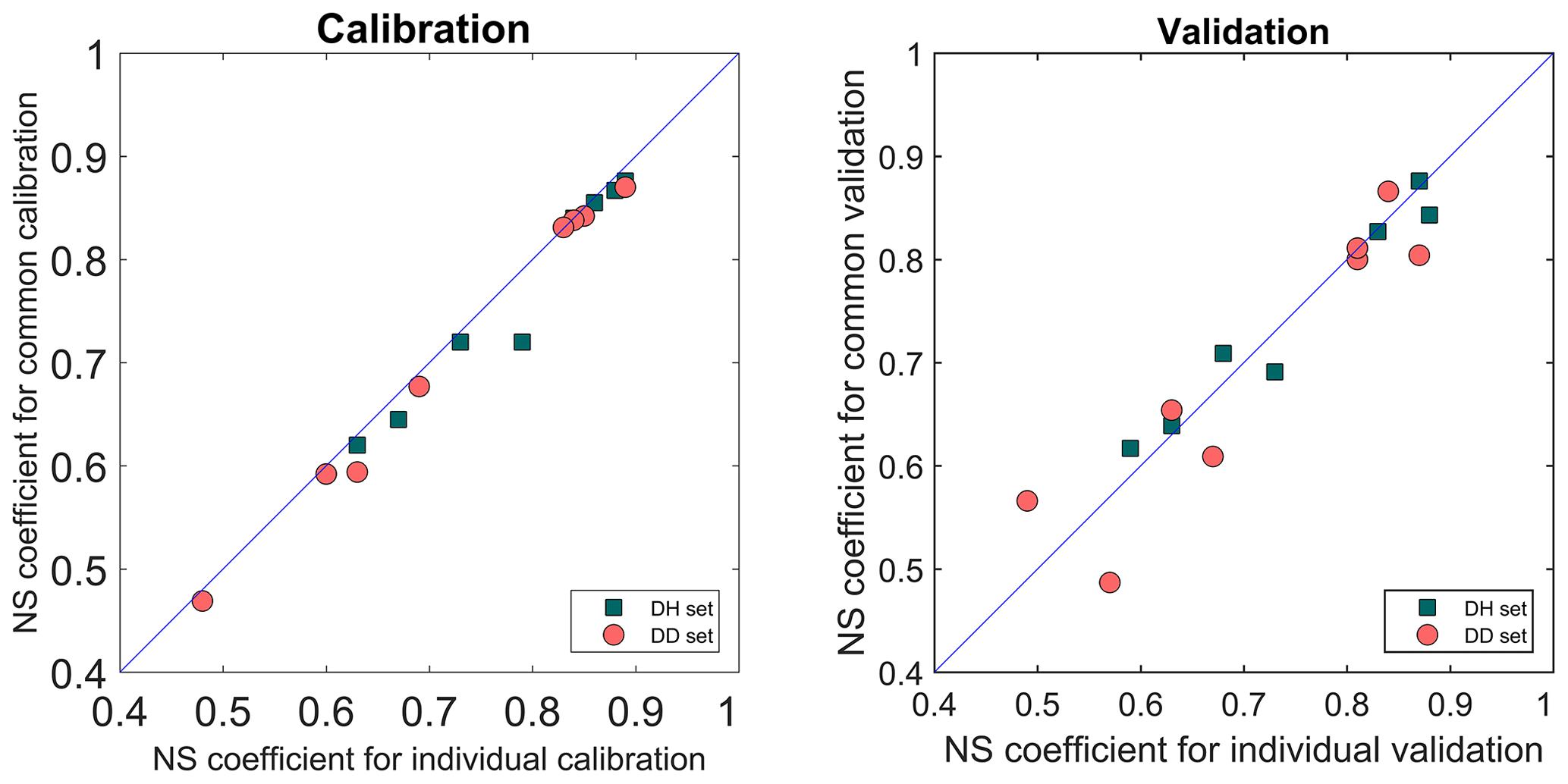
Figure 14 Comparison of the NS coefficient for individual calibration and common calibration using datasets with different temporal resolutions.

The calibrated model parameters using daily rainfall, hourly rainfall and a common calibration strategy were also compared. Figures 15 and 16 show the distributions of the optimized model parameters for Rottweil and Pforzheim, respectively. Note that all parameters are normalized by the initial ranges in Table 2. From the boxplots we could find that some model parameters strongly depend on the selected rainfall dataset. This is very evident with the shape factor (Beta) and the threshold water level for surface runoff (L).

Figure 15 Comparison of model parameters for different temporal resolutions for Rottweil catchment.

Figure 16 Comparison of model parameters for different temporal resolutions for Pforzheim catchment.

5 Conclusions and outlook

In this study, we investigated the impacts of temporal and spatial variability of rainfall in model simulation and parameter estimation. We also explored the question whether higher temporal and spatial resolutions of rainfall data lead to any improvement in model performance. Both the lumped and spatially distributed HBV model were applied to simulate daily runoff for four mesoscale catchments driven by four different rainfall datasets which were constructed using a combination of data from a high density of daily stations and relatively low-density sub-daily stations. The impacts of rainfall variability on model simulations were evaluated using the NS coefficient and the mean squared error of flows higher than the 10th percentile of flow. The model sensitivities to the temporal and spatial resolutions of rainfall were compared. In addition, the common calibration approach was proposed to calibrate the models with different time steps simultaneously for finding robust model parameters.

For the study catchments, the results indicate that the temporal variability of rainfall data has direct impact on the dynamic response of a catchment. For both lumped and spatially distributed models, if the observation density is the same, the hourly based simulation outperforms the daily based simulation, indicating that higher temporal resolution can significantly improve the model performance. Disaggregating high-density daily observations into relatively low-density sub-daily values could lead to considerable model improvement, especially for the catchment with a sparse raingauge network. The rainfall disaggregation approach is an effective way of increasing the temporal resolution of rainfall data and the model performance. However, the lumped and spatially distributed HBV models perform very similarly, indicating that higher spatial resolution does not improve or only marginally improves the model performance for the study catchments. The result agrees with the general findings of Lobligeois et al. (2014) and Zhu et al. (2018), where insignificant improvement was observed using higher spatial resolution of rainfall. The reason that the spatially distributed model does not outperform the lumped model could be due to the fact the study catchments are smaller than 2000 km² with relatively uniform rainfall.

As stated at the beginning of this paper, we aim to investigate the sensitivity of the model to rainfall variability and to find effective ways of improving the model performance. This study shows that rainfall data disaggregation can lead to a significant improvement in model performance, while higher spatial resolution of rainfall does not always enhance model performance. Most of the hydrological models can be easily adjusted to use different time steps. The study suggests that increasing the temporal resolution of rainfall inputs with the disaggregation method can be an easier and more efficient way to improve model performance, compared to increasing the model spatial resolution at a cost of increasing the complexity of model structure and parameters.

This study focuses on high flows and uses only the NS coefficient as a quantitative measure of model sensitivity. As model performance highly depends on the selection of objective functions, the model sensitivity can be different if the model performance is measured differently. In addition, all the hourly simulated runoff was aggregated into daily runoff, and the hydrological response was evaluated based on daily discharge. Sub-daily response of a catchment is more sensitive to the temporal and spatial variability of rainfall, which should be considered in the future if the hourly discharge observation is available.