High-resolution paleovalley classification from airborne electromagnetic imaging and deep neural network training using digital elevation model data

Paleovalleys are buried ancient river valleys that often form productive aquifers, especially in the semiarid and arid areas of Australia. Delineating their extent and hydrostratigraphy is however a challenging task in groundwater system characterization. This study developed a methodology based on the deep learning super-resolution convolutional neural network (SRCNN) approach, to convert electrical conductivity (EC) estimates from an airborne electromagnetic (AEM) survey in South Australia to a high-resolution binary paleovalley map. The SRCNN was trained and tested with a synthetic training dataset, where valleys were generated from readily available digital elevation model (DEM) data from the AEM survey area. Electrical conductivities typical of valley sediments were generated by Archie's law, and subsequently blurred by down-sampling and bicubic interpolation to represent noise from the AEM survey, inversion and interpolation. After a model training step, the SRCNN successfully removed such noise, and reclassified the low-resolution, converted unimodal but skewed EC values into a high-resolution paleovalley index following a bimodal distribution. The latter allows us to distinguish valley from non-valley pixels. Furthermore, a realistic spatial connectivity structure of the paleovalley was predicted when compared with borehole lithology logs and a valley bottom flatness indicator. Overall the methodology permitted us to better constrain the three-dimensional paleovalley geometry from AEM images that are becoming more widely available for groundwater prospecting.

1 Introduction

A paleovalley is the remnant of an inactive ancient river valley filled by unconsolidated, semi-consolidated or lithified sediments, which often have a higher porosity and permeability than the surrounding rocks (Jackson, 2005). Paleovalleys are important in mineral exploration as they may contain remobilized gold, uranium, and heavy minerals (Hou et al., 2008) and in groundwater exploration, as they often form productive aquifers (Samadder et al., 2011; Mulligan et al., 2007; Knight et al., 2018). However, delineating the geometry and connectivity of paleovalleys at the regional scale (tens to hundreds of kilometers) with a high resolution (tens of meters in horizontal plane) is challenging (Holzschuh, 2002; Lane, 2002). This is mainly because surface geophysical surveys and borehole data often do not yield the required spatial resolution and coverage to reliably and cost-effectively map connected paleovalleys at a regional scale.

Aerial geophysical surveys, such as airborne electromagnetic (AEM) surveys, can be inverted to provide depth profiles of electrical conductivity (EC) at a regional scale over tens to hundreds of kilometers (Fitterman et al., 1991). Their horizontal resolution depends on the distance between flight lines (typically between 250 m and 30 km), which can be tailored to the problem at hand, while vertical resolution ranges from meters to tens of meters. Classification of geophysical properties into paleovalleys and non-valley zones is most often done manually, although several methods have been developed to automate the identification of lithofacies from electrical conductivity estimates. Most of these methods assume a simplified petrophysical relationship between electrical conductivity and hydraulic parameters (e.g., porosity and permeability) (Vilhelmsen et al., 2014; Marker et al., 2015; Pollock and Cirpka, 2010). Using synthetic borehole data, Christensen et al. (2017) converted AEM data to lithofacies at a scale of kilometers by use of Markov Chain Monte Carlo and sequential indicator simulation methods.

Electrical conductivity values estimated from AEM surveys are subject to uncertainties introduced by variations in land cover during surveys, inversion processes, and the interpolation of EC values to the required resolution (Viezzoli et al., 2008; Robinson et al., 2008). Consequently, the relationship between EC and lithofacies is complex and difficult to identify. In this paper, we introduce a deep-learning (neural network)-based methodology (including training dataset generation, and neural network construction and training) for automatic classification of high-resolution binary paleovalley maps from AEM-derived EC data with noise.

Artificial neural networks (ANNs), which can express the complex and nonlinear relationship between input and outputs, were previously applied for the inversion of EC values from original AEM data (Ahl, 2003) and to classify lithology from AEM-derived EC data (Gunnink et al., 2012). However, the large number of weights involved in ANN make it difficult to train the network and often leads to overfitting problems (Tu, 1996). Deep learning approaches based on convolutional neural networks with sharing weights were established in 2006 (Gu et al., 2017), and are now well accepted in the field of visual recognition, speech recognition and language processes. They provide efficient high-dimensional interpolators that cope with multiple scales and heterogeneous information (Marcais and de Dreuzy, 2017), and have been applied in geoscience for earthquake detection based on seismic monitoring (Perol et al., 2018), object and disaster recognition from remote-sensing data (Längkvist et al., 2016; Amit et al., 2016), and mineral prospectivity evaluation by the fusing of different geophysical datasets (Granek, 2016; Meller et al., 2013). Furthermore, a super-resolution convolutional neural network (SRCNN) approach composed merely of convolutional layers was established to directly capture the relationship between low- and high-resolution images (Dong et al., 2016). The SRCNN was found to be accurate, robust and fast for removing noise from low-resolution images and reconstructing a super-resolution image (Hao et al., 2018; Tuna et al., 2018; Luo et al., 2017).

In this study, concepts from the SRCNN approach are used to identify paleovalleys at high spatial resolution from a regional-scale AEM survey. The objective is to develop a methodology based on SRCNN to generate a high-resolution, regional-scale map of paleovalleys from low-resolution AEM-derived EC data that (1) reproduces paleovalley connectivity and (2) accounts for noise in the EC data. The method is applied to an arid region of South Australia to identify paleovalleys at depths up to 100 m, i.e., the depth up to which the AEM-derived EC has a sufficient signal-to-noise ratio. The paper is organized as follows; Sect. 2 presents the data availability in our study area. Section 3 introduces the methodology, which is followed by performance analyses in Sect. 4. Section 5 concludes the major findings.

2 Study area and dataset

Australian landscapes are ancient, featuring the product of subdued tectonics, long-term subaerial exposure and an extremely limited extent of Quaternary glaciation. This often manifests itself in an extensive paleovalley network with deep weathering profiles and thick accumulation of unconsolidated alluvium and colluvium. The widespread paleovalley networks in today's arid landscape are remnants of the Early Cenozoic inset valleys with Tertiary sedimentary infill and a thin and variable Quaternary cover (Magee, 2009). In the intracontinental Cenozoic sedimentary basins, paleovalley infill sediments typically consist of Eocene sediments overlain by more finely grained sediments of Oligocene to Miocene age. The Eocene sediments are dominantly coarsely grained fluvial sands and basal gravels, deposited under wet climatic conditions. The Oligocene to Miocene sediments were deposited by relatively lower-energy drainage systems under drier climatic conditions. During the Quaternary, eolian sediments with maximum observed thickness of 15 m covered portions of the paleovalleys at a time when fluvial or lacustrine deposition had ceased (Magee, 2009).

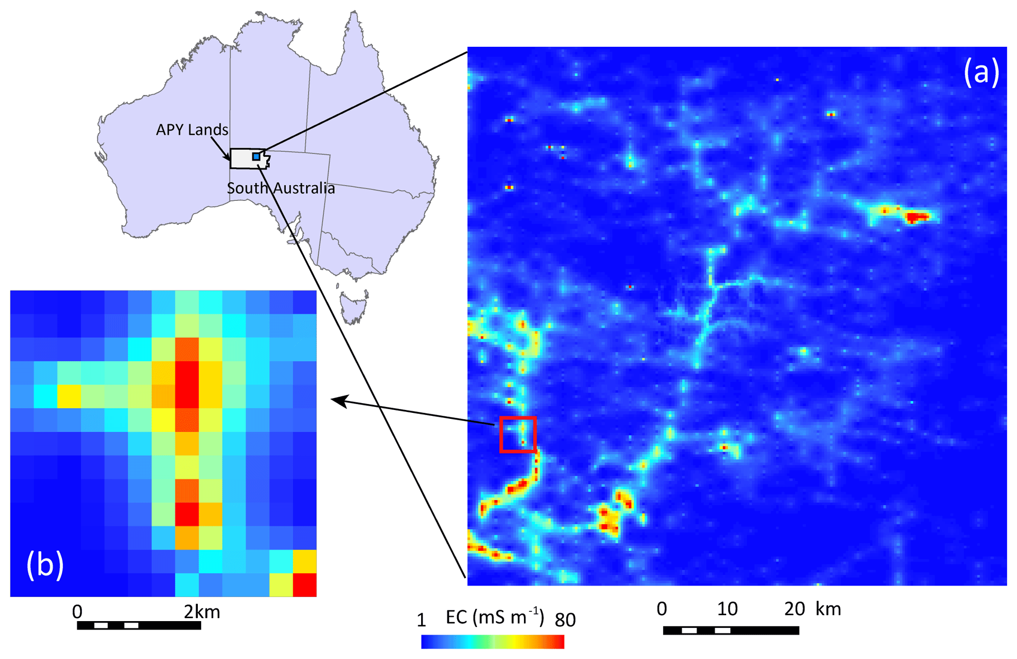
Figure 1 (a) Electrical conductivity at 100 m depth ranging from 1 to 80 mS m⁻¹, as interpreted from airborne electromagnetic surveys in the Anangu Pitjantjatjara Yankunytjatjara (APY) lands, Australia; (b) inset shows details of EC map at a spatial resolution of 400 m ×400 m (Soerensen et al., 2016).

This study focuses on the Anangu Pitjantjatjara Yankunytjatjara (APY) lands, which are part of the Musgrave province in northern South Australia (Fig. 1). This area features an arid climate with very low and unreliable rainfall averaging about 230 mm yr⁻¹ (Jones et al., 2009). However, an extensive paleovalley system with sedimentary faces aligning with the Cenozoic sedimentary basins above represents a shallow dynamic groundwater system exhibiting reliable water resources for local communities and mining (English et al., 2012; Munday et al., 2013).

Within the study area 128 bores, drilled between 1970 and 2018, with lithological information were retrieved from the South Australia Government WaterConnect database (https://www.waterconnect.sa.gov.au/Pages/Home.aspx, last access: 3 January 2019). Three lithological classes were derived from the logs.

1. Bedrock. Basement at surface or covered with in situ weathering products (clays, broken basement fragments).

2. Alluvium (sediments in paleovalleys). Basement covered with more than 15 m of unconsolidated sediments consisting of sand and gravel with minor silt and clay, showing indication of alluvial sediment transport.

3. Transition. Basement covered with up to 15 m of eolian sands or lacustrine sediments consisting of silt and clay with minor amounts of sand or gravel, showing limited indication of transport.

While the information content in these logs was often limited, they provided independent lithological data to verify the predicted paleovalley network in this study (see further).

Two AEM surveys were flown in the APY lands in 2016, covering a total area of 33 500 km² and featuring a line spacing of 2 km in the north–south direction (Soerensen et al., 2016). An area 80 km by 80 km in a central-east section of the APY lands is selected and used to test mapping paleovalleys based on a SRCNN analysis of electrical conductivity (EC) generated from the AEM survey (Fig. 1). In this area, the AEM survey was undertaken using the helicopter-borne SkyTEM^312FAST system (Soerensen et al., 2016). The averaging trapezoidal filter was used to reduce the noise in low- and high-moment amplitude response data. Aarhus Workbench software was used to invert AEM data to obtain EC (Auken et al., 2009, 2014). In a final step, ordinary kriging was used to interpolate EC values to a spatial resolution of 400 m × 400 m in the horizontal plane and 10 m in the vertical cross section (Ley-Cooper and Munday, 2013; Soerensen et al., 2016). The constraint on the lateral resolution of the AEM data was determined by the line spacing of the survey (2 km). In the APY lands, it was gridded to a cell size of a fifth of the line spacing (i.e., 400 m), to maintain the fidelity. The depth interval is commonly between 5 and 10 m increasing exponentially with depth because AEM is a diffusive technology (Yang et al., 2013; Spies, 1989). In the APY lands the vertical resolution is 10 m for the first 100 m depth interval to avoid generating too many interval conductivity slices. Only the EC values in the first 10 depth slices, up to 100 m depth, are used in this study to construct the binary paleovalley pattern per slice, which are then stacked up to a quasi-3-D image of the paleovalley.

Bulk electrical conductivity of the subsurface depends on both the solid phase (i.e., the rock mass) and the liquid phase (i.e., soil water and groundwater). It is further influenced by the porosity, tortuosity of the pore space and degree of water saturation. Unweathered rocks are generally a poor electrical conductor with EC values typically less than 1 mS m⁻¹ for igneous and metamorphic rock, and 1 to 1000 mS m⁻¹ for regolith (e.g., gravel, sand, silt and clay) (Lane, 2002); saline groundwater with a salinity level similar to seawater has an EC of around 3000–5000 mS m⁻¹, while freshwater EC is up to 150 mS m⁻¹ (Lane, 2002; Rhoades et al., 1976; Purvance and Andricevic, 2000).

Previous hydrogeological characterization studies in the APY lands study area indicated that paleovalley porosity values are relatively high (from 10 % to 30 %) with the mean salinity of the pore fluid reaching 4500 mg L⁻¹ (700 mS m⁻¹); the surrounding rocks (fractured granites and gneiss) have a much lower porosity (< 1 %) and water salinity values (< 1000 mg L⁻¹, 160 mS m⁻¹ ) (Varma, 2012; Taylor et al., 2015). It is reasonable to assume that a clear distinction exists in this study area between EC values of the valley and non-valley lithologies, and thus only EC is used to distinguish paleovalleys from surrounding basement. However, due to the data smoothing methods used during inversion of the AEM data and EC interpolation, and the continuous variation in water salinity near the interface between paleovalley and fractured bedrocks, the resulting EC values vary continuously (Fig. 1b), which makes the boundary between valley and non-valley lithologies rather diffuse. Our novel methodology allows us to automatically identify the boundaries between valley and non-valley lithologies based on convolutional neural networks.

3 Methodology

The method developed in the present study to identify paleovalleys is comprised of three key steps. (1) A deep neural network training dataset is generated by creating synthetic paleovalley networks from a digital elevation model (DEM) of the study area; the paleovalley network is converted to EC values by applying Archie's law (see further) to the water-bearing formations, while EC values for the non-valley zone composed of fractured bedrock are obtained as a volume-weighted average of EC values of rock and fluid components; (2) the SRCNN is trained and validated using the synthetic EC and corresponding paleovalleys to remove noise and establish a nonlinear relationship between the EC image and paleovalley image; (3) the SRCNN is then applied to predict the paleovalley in the APY lands based on measured AEM data. The algorithm of training dataset generation and SRCNN and the performance metrics to evaluate SRCNN paleovalley classification are described in detail below.

3.1 Synthetic training data generation

Australia is well known for its relative tectonic stability and is a stable continent located in an intraplate position. The paleovalley networks are coherent, dominantly dendritic, and largely concordant with modern topographic expression (Magee, 2009). Although paleovalleys in the arid zone are partly covered by Quaternary eolian deposits, the topographic expression of the paleovalley pattern is still evident in high-resolution digital elevation model (DEM) data (Magee, 2009). In the APY lands, crustal architecture has been preserved since the Cenozoic, and it is considered to have been unaffected by later tectonic events (Drexel and Preiss, 1995). Previous studies in the study area have considered that the paleovalleys are coincident with topographic lows that characterize the contemporary landscape, with AEM images being particularly useful for locating the position of the deeper portions of the older valley system (Munday et al., 2013). It is thus assumed that the present-day valley pattern indicated by topographic lows in the study area is comparable to the paleovalley pattern according to the principle of uniformitarianism (Simpson, 1970), but shifts in valley width, orientation and connectivity between present-day valley and paleovalley are allowed. Following this principle, we generate a synthetic paleovalley image based on a digital elevation model (DEM).

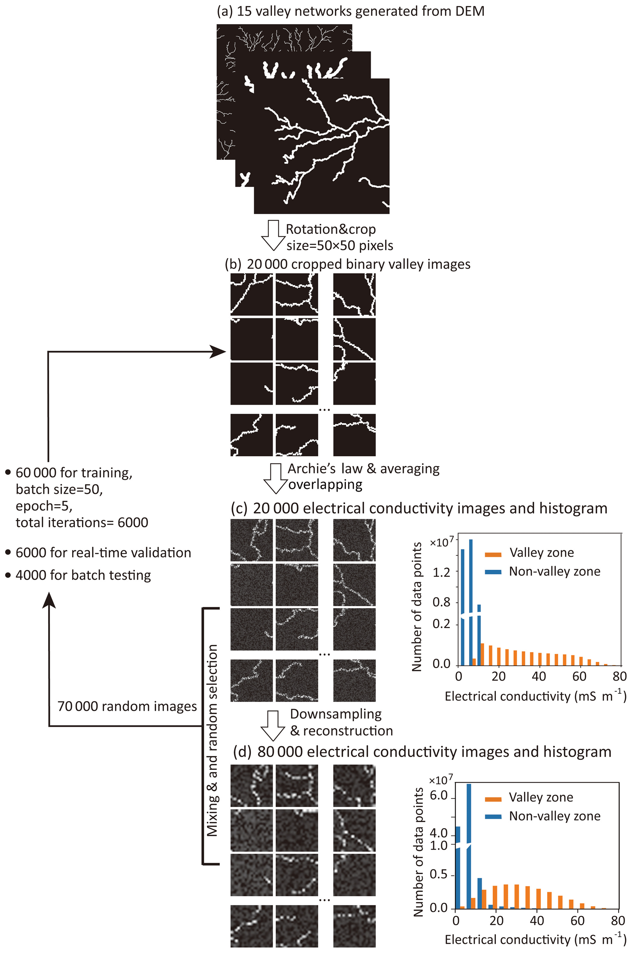
Figure 2 Workflow diagram of methodology used to generate training and validation datasets. (a) Synthetic paleovalley networks generated from DEM data of the study area. (b) Rotation and cropping to randomly generate 20 000 sub-images from 15 initial paleovalley networks. (c) Conversion of valley images to EC values using Archie's law in valley and weighted averaging in non-valley zone. (d) Down-sampling of resulting 50×50 pixel EC spatial distributions to 10×10 pixel resolution (20 000), 20×20 pixels (20 000), 30×30 pixels (20 000) and 40×40 pixels (20 000), respectively, and reconstructed to obtain 80 000 blurred EC images. A total of 70 000 EC images are randomly selected from original EC images (c) and reconstructed EC images (d), forming 70 000 image pairs including 20 000 binary valley images (with some EC images corresponding to the same valley image) to train the SRCNN.

First, a DEM of the study area with a resolution of 30 m ×30 m (https://earthexplorer.usgs.gov/, last access: 23 December 2018) is used to generate 15 sets of paleovalley images, mimicking paleovalleys of various spatial densities and width over an area of 80 km ×80 km based on the hydrological analysis in ArcGIS (Fig. 2a) (details in Maidment and Morehouse, 2002). For convenience in the subsequent neural network operation, each resulting valley image is downscaled by the bicubic interpolation method to contain 800×800 pixels with spatial resolution of 100 m. Valley widths range from 1 to 10 pixels (i.e., 100 to 1000 m). The 15 images generated from the DEM were rotated between zero and 360^∘ and randomly cropped into 20 000 small training images with a size of 50×50 pixels (Fig. 2b). Thus, the potential differences in the width and orientation of present-day valley and paleovalley induced by several uncertain factors, e.g., variation in the river discharge and geomorphology, can be addressed in the training images. The recombination of small training images allows recreation of valley patterns beyond those 15 full-size images generated from DEM data. A broad range of likely paleovalley patterns at varying principle orientations, widths and connectivity are available in the SRCNN training image pool.

The properties in the porous paleovalley sediments are then converted to EC values using Archie's law (Archie, 1942):

$$\begin{array}{}\text{(1)}& {\displaystyle }R=R_{\mathrm{0}}{\mathit{\theta }}^{-m},\end{array}$$

where R is the electrical resistivity of the water-bearing formation (Ωm), R₀ is the electrical resistivity of the pore water relating to water salinity (Ωm), θ is the porosity and m is a constant relating to the lithology (with value ranging from 1.8 to 2.0) (Worthington, 1993). Electrical conductivity values are calculated as the inverse of resistivity values (i.e., EC $=\mathrm{1}/R$). In the present study area, R₀ is considered to range from 1.4 to 1.7 Ωm, corresponding to water salinities of 3000 to 6000 mg L⁻¹ (Varma, 2012), while θ is considered to range from 10 % to 30 % (Taylor et al., 2015; Varma, 2012). As a result, paleovalley EC values are estimated to be within the range of 6 to 80 mS m⁻¹, which is in the range of AEM-derived EC values in Fig. 1.

In contrast, the non-paleovalley zone is predominantly fractured rock with solid-phase EC values < 1 mS m⁻¹, characteristic porosity of < 1 % and fluid salinity values of < 150 mS m⁻¹ EC (1000 mg L⁻¹) (Olhoeft, 1981; Parkhomenko, 2012). The bulk EC values in the non-paleovalley zones were estimated as the volume-weighted average of EC in fractured rock and fluid, following

$$\begin{array}{}\text{(2)}& {\displaystyle }\mathrm{EC}={\mathrm{EC}}_s\cdot \left(\mathrm{1}-\mathit{\phi }\right)+{\mathrm{EC}}_{\mathrm{f}}\cdot \mathit{\phi },\end{array}$$

where EC is the bulk electrical conductivity, EC_s is the EC value of rocks, EC_f is the EC of fluid and φ is the ratio of fracture void volume to total volume. The resulting bulk EC values are lower than 2.5 mS m⁻¹. Again, these synthetic EC values are similar to the AEM-derived values for the presumed fractured bedrock areas (Fig. 1).

Furthermore, to represent the effects from data smoothing and inherent noise associated with the AEM survey, inversion and data interpolation, artificial noise is generated by randomly sampling EC values in the non-paleovalley zones (following a uniform distribution ranging from 1 to 10 mS m⁻¹) and in the paleovalley zones (following a uniform distribution ranging from 6 and 80 mS m⁻¹). It is also noted that the upper-limit EC values in fractured bedrock areas are enlarged artificially from 2.5 to 10 mS m⁻¹, to assure that in the training images paleovalley and non-paleovalley zones overlap in EC by 4 mS m⁻¹ (5 % of the total range of EC values between 1 and 80 mS m⁻¹) (Fig. 2c). The SRCNN can then learn to identify this overlap in EC between paleovalley and non-valley zones. However, Appendix A1 shows that setting the overlapping size in EC too large results in the trained SRCNN overestimating the extent of the non-valley zones, which make the predicted paleovalleys disconnected.

The overlap in EC near the boundary between paleovalley and non-valley is further enhanced by data smoothing: the resultant EC images of 50×50 pixels is first downscaled into images with a smaller number of pixels, i.e., 40×40 (20 000 images), 30×30 (20 000 images), 20×20 (20 000 images) and 10×10 (20 000 images) pixels, respectively, by nearest-neighbor interpolation. These resulting 80 000 images are then upscaled by bicubic interpolation to yield blurred images with the original resolution of 50×50 pixels (Fig. 2d). In this manner, the EC values in the paleovalley and non-paleovalley zones are smoothed and the boundary between paleovalley and non-paleovalley becomes blurred.

We then randomly selected 70 000 EC images from a total of 100 000 images, composed of 20 000 pre-interpolation EC images (Fig. 2c) and 80 000 reconstructed blurred EC images (Fig. 2d) with a size of 50×50 pixels, as input to the neural network (see further), with the original synthetic paleovalley images (pixel code 1) and non-paleovalley (pixel code 0) pixels (Fig. 2b) as output. From the random set of 70 000 images, 60 000 pairs of EC (Fig. 2c and d, as input) and paleovalley images (Fig. 2b, as output) are used as a “training dataset” for training the SRCNN. A total of 6000 pairs are used as “validation dataset” for validation and another 4000 are used as “testing dataset” to demonstrate the performance of the trained SRCNN in removing the noise in EC images and lithofacies (paleovalley and non-paleovalley) classification.

3.2 SRCNN algorithm

To quantify the relationship between EC images and paleovalley images, the super-resolution convolutional neural network (SRCNN) algorithm is employed. Neural networks are regression models that provide a general way of identifying nonlinear relationships between two sets of variables (Bishop, 1996; Moysey et al., 2003), where one set of variables is considered to be the input (herein electrical conductivity) and another is a network output (binary paleovalley). The SRCNN algorithm can directly train the relationship between a low-resolution (input) and a high-resolution image (output) (Dong et al., 2016). A typical SRCNN is composed of three convolution layers (Fig. 3), representing patch extraction and representation, nonlinear mapping, and reconstruction.

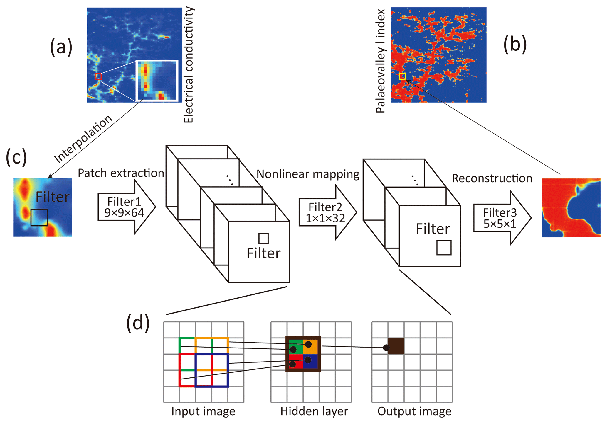
Figure 3 Algorithm of converting (a) low-resolution EC image to (b) high-resolution paleovalley image based on (c) the super-resolution convolutional neural network. (d) Convolutional processes of data from an input image to an output image by a filter with a size of 2, moving through the input image 1 pixel at the time.

In the patch extraction and representation layer, the input is a normalized 50×50 pixel EC image, which is operated by a convolution process:

$$\begin{array}{}\text{(3)}& {\displaystyle }{\mathbf{H}}^{\mathrm{1}}\left(\mathbf{X}\right)=\max \left(\mathrm{0},〈{\mathbf{XW}}^{\mathrm{1}}〉+{\mathit{b}}^{\mathrm{1}}\right),\end{array}$$

where H represents the output images, <> is the convolution operator, X represents the input EC image, and W and b represent the weight filter and bias, respectively. W¹ corresponds to n₁ filters with a size of f₁×f₁ and b¹ is an n₁-dimensional vector. After convolution, H¹ contains n₁ generated 50×50 pixel images that are input into the nonlinear mapping layer. It is then convoluted by

$$\begin{array}{}\text{(4)}& {\displaystyle }{\mathbf{H}}^{\mathrm{2}}\left({\mathbf{H}}^{\mathrm{1}}\right)=\max \left(\mathrm{0},〈{\mathbf{H}}^{\mathrm{1}}{\mathbf{W}}^{\mathrm{2}}〉+{\mathit{b}}^{\mathrm{2}}\right)\end{array}$$

to generate H² composed by n₂ 50×50 pixel images, where W² contains n₂ filters with a size of $n_{\mathrm{1}}\times f_{\mathrm{2}}\times f_{\mathrm{2}}$ and b² is a n₁×n₂ matrix.

Finally, an output paleovalley index (with values approaching zero indicating a non-valley pixel and values approaching unity indicating a paleovalley pixel) can be reconstructed from H² by

$$\begin{array}{}\text{(5)}& {\displaystyle }{\mathbf{H}}^{\mathrm{3}}\left({\mathbf{H}}^{\mathrm{2}}\right)=G\left(〈{\mathbf{H}}^{\mathrm{2}}{\mathbf{W}}^{\mathrm{3}}〉+{\mathit{b}}^{\mathrm{3}}\right).\end{array}$$

H³ contains one 50×50 pixel paleovalley index image, and W³ contains one filter with a size of $n_{\mathrm{2}}\times f_{\mathrm{3}}\times f_{\mathrm{3}}$ and b² is a n₂×1 matrix. G(⋅) is a sigmoid function to assist the paleovalley classification and accelerate the training processes, which is written as

$$\begin{array}{}\text{(6)}& {\displaystyle }G\left(\cdot \right)=\exp (\cdot )/[\mathrm{1}+\exp (\cdot \left)\right].\end{array}$$

In this study, f₁, f₂ and f₃ are referred to as filter size with values of 9, 1 and 5, respectively, and n₁ and n₂ are the layer width (the number of images contained in each layer) with values of 64 and 32, respectively, following the classical structure of SRCNN used in Dong et al. (2016). The influence of the filter size and width on the quality of the output images was investigated in Appendix A3. The filter size in the SRCNN controls the spatial correlation length of EC values that can be considered in the neural network operator. As illustrated in Fig. 3d, in each calculation, the EC values in the filter are convoluted to form a value at a single pixel in the output image. An EC image convoluted by the filter with the size of 2 and stride of 1 (i.e., filter moving 1 pixel at the time) and one hidden layer, leads to a paleovalley index at 1 pixel of the output image that relates to EC values from 3×3 pixels in the input image. In this example, the spatial correlation scale able to be addressed is equal to 3 pixels multiplied by the size of each pixel (meter). In addition, the width of each layer determines the degree of the nonlinear relationship between input and output, while the depth of the network affects both the spatial correlation length and the nonlinearity (see further in Appendix A3).

The initial weight values are randomly generated, following a standard normal distribution, while initial bias values are given as 0.1. Both weight and bias values for each of the three convolutional neural network layers are optimized simultaneously using the adaptive moment estimation algorithm (Kingma and Ba, 2014) to minimize the loss function, L, which is defined as the mean sum of squared residuals:

$$\begin{array}{}\text{(7)}& {\displaystyle }L\left({\mathbf{W}}^{\mathrm{1}},{\mathbf{W}}^{\mathrm{2}},{\mathbf{W}}^{\mathrm{3}},{\mathit{b}}^{\mathrm{1}},{\mathit{b}}^{\mathrm{2}},{\mathit{b}}^{\mathrm{3}}\right)={\displaystyle \frac{\mathrm{1}}{N}}\sum _{i=\mathrm{1}}^N{∥{\mathbf{H}}^{\mathrm{3}}-\mathbf{Y}∥}^{\mathrm{2}},\end{array}$$

where Y is the known binary paleovalley pattern (0 represents non-paleovalley, 1 corresponds to the paleovalley) in the training data, and N is the number of image pixels in each training.

3.3 Performance metrics of the SRCNN algorithm

To verify the performance of the SRCNN, the following image quality indices are calculated.

1. Peak signal-to-noise ratio (PSNR) (Wang and Bovik, 2002):

   $$\begin{array}{}\text{(8)}& {\displaystyle }\mathrm{PSNR}=-\mathrm{10}{\log }_{\mathrm{10}}\left[{\displaystyle \frac{\mathrm{1}}{N}}\sum _{i=\mathrm{1}}^N({\stackrel{\mathrm{̃}}{Y}}_i-Y_i{)}^{\mathrm{2}}\right],\end{array}$$

   where Y represents the synthetic binary paleovalley index generated from the DEM (0 for non-paleovalley and 1 for paleovalley) (Fig. 2b) and $\stackrel{\mathrm{̃}}{Y}$ is the calculated paleovalley index (Eq. 5) from SRCNN using EC images as input, and the term between brackets is the mean square error. PSNR is a traditional approach to image quality assessment. A high PSNR represents a high-quality paleovalley generation; e.g., a PSNR =20 value is equivalent to a mean-square error of 0.01.

2. Structure similarity index (SSIM) (Wang et al., 2004):

   $$\begin{array}{}\text{(9)}& {\displaystyle }\mathrm{SSIM}={\displaystyle \frac{\mathrm{2}{\mathit{\mu }}_Y{\mathit{\mu }}_{\stackrel{\mathrm{̃}}{Y}}+\mathit{\epsilon }}{{\mathit{\mu }}_Y^{\mathrm{2}}+{\mathit{\mu }}_{\stackrel{\mathrm{̃}}{Y}}^{\mathrm{2}}+\mathit{\epsilon }}}\cdot {\displaystyle \frac{\mathrm{2}\mathrm{cov}\left(Y,\stackrel{\mathrm{̃}}{Y}\right)+\mathit{\epsilon }}{{\mathit{\sigma }}_Y^{\mathrm{2}}+{\mathit{\sigma }}_{\stackrel{\mathrm{̃}}{Y}}^{\mathrm{2}}+\mathit{\epsilon }}},\end{array}$$

   where μ is the mean,  σ² the variance, and cov(⋅) the covariance of the synthetic or calculated paleovalley index and ε is a small number (10⁻⁶). SSIM is complementary to PSNR, but focuses on structural similarity between a reference and distorted image. It ranges theoretically from 0 to 1.0. The higher the SSIM, the higher the resolution of the paleovalley network being reconstructed.

3. Connectivity function (Pardo-Igúzquiza and Dowd, 2003; Renard and Allard, 2013):

   $$\begin{array}{}\text{(10)}& {\displaystyle }\mathit{\tau }\left(h\right)={\displaystyle \frac{N\left(u\leftrightarrow u+h\mathrm{|}u,u+h\in S\right)}{N\left(u,u+h\in S\right)}},\end{array}$$

   where $N(uu+h\in S)$ is the number of paleovalley pixels in a certain direction within the distance h, while $N(u\leftrightarrow u+h\mathrm{|}uu+h\in S$) is the number of connected paleovalley pixels in this direction. It ranges from 0 to 1.0, and high values indicate a strong spatial connectivity.

4 Results and discussion

We here (1) monitor both PSNR and SSIM between the paleovalley index generated from SRCNN and DEM for 60 000 training and 6000 validation datasets to test for the overfitting problem; (2) generate paleovalley index maps from synthetic EC images in 4000 testing datasets to demonstrate the performance of SRCNN in identifying the noise in EC images and classification and recreate the connectivity of the paleovalley; (3) infer binary paleovalley maps by applying the trained SRCNN to the AEM-based EC values in the study area; and (4) compare the resulting paleovalley image with borehole lithology logs and existing paleovalley indicators, i.e., multiple-resolution valley bottom flatness.

4.1 Training and preliminary testing

The training dataset composed of 60 000 pairs of EC and valley images in Fig. 2 is divided into 1200 batches (inner number of iterations) with each batch containing 50 images. The epoch (outer number of iterations) is set to 5, and the 60 000 training image pairs are resorted at the beginning of each epoch. In this scenario, weights and biases in the SRCNN are updated by 6000 iterations (5×1200), according to the loss function calculated based on 50 pairs of images in each batch.

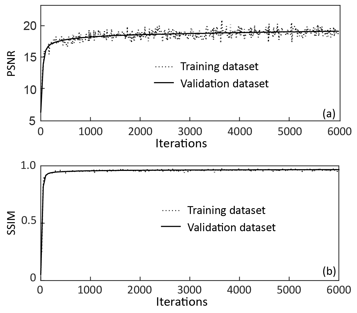
Figure 4 (a) PSNR and (b) SSIM values between paleovalley index generated from SRCNN and DEM recorded for both training (60 000 images) and validation (6000 images) datasets. For SRCNN training 50 images are used per iteration.

After each iteration, the PSNR (Eq. 8) and SSIM (Eq. 9) for 50 training images in each batch are calculated (Fig. 4a and b). Moreover, the PSNR and SSIM for 6000 validation images are calculated for every 50 iterations. It is illustrated that PSNR for each training batch fluctuates near 18 (which corresponds to a mean-square error of 0.015 based on Eq. 8), while the SSIM stabilizes at 0.96. The PSNR and SSIM values for the validation images agree well with those of the training images. This suggests that the SRCNN is sufficiently trained to recreate the paleovalley with a high accuracy without overfitting problems, and importantly preserving structural similarity.

4.2 Performance of SRCNN for noise removal, lithofacies classification and recreating connectivity

The trained SRCNN is then applied to generate paleovalley images based on 4000 testing EC images; we here randomly selected four images to demonstrate the ability of SRCNN. The synthetic paleovalley images from DEM and their corresponding blurred EC images are illustrated in Fig. 5a and b, respectively. The histogram of EC values for all 4000 images (each containing 50×50 pixels) in the testing dataset follows a unimodal, right-skewed distribution (Fig. 5c). It is not trivial to define an EC threshold value from such unimodal distribution that can be used to distinguish the paleovalley and non-paleovalley cells from Fig. 5b. After calibration of the SRCNN, a paleovalley index map is obtained (Fig. 5d). However, the histogram of the resultant paleovalley index displays a bimodal behavior, with peaks centered at 0 and 1 (Fig. 5e). By selecting a threshold paleovalley index value of 0.5, the paleovalley and the non-paleovalley data can be differentiated and converted to a binary paleovalley map (Fig. 5f). The resultant paleovalleys compare well with the reference (i.e., synthetic) paleovalleys in Fig. 5a. The selection of a threshold paleovalley index in the range of 0.2 to 0.8 does not have a significant influence on the resultant binary paleovalley pattern.

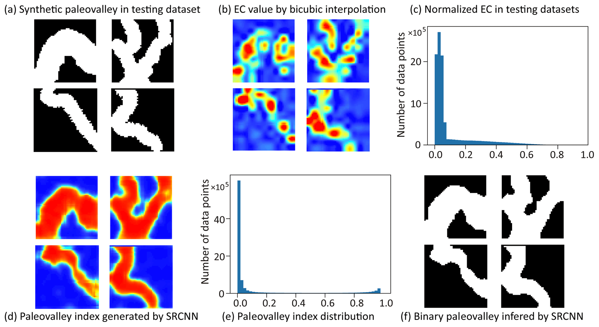
Figure 5 (a) DEM-generated synthetic paleovalley used as reference image in testing the SRCNN; (b) normalized electrical conductivities corresponding to the paleovalleys following (c) a skewed distribution (based on 4000 images in the test dataset). (d) Paleovalley index generated through processing EC images via the SRCNN; (e) bimodal distribution of paleovalley index (based on 4000 images in the test dataset); (f) the paleovalley index map converted into a binary paleovalley map by arbitrarily selecting the paleovalley index threshold as 0.5.

Moreover, the resultant paleovalley index is less noisy in both paleovalley and non-paleovalley parts (Fig. 5d). The SRCNN is able to create connected paleovalley networks from the poorly connected EC values generated by bicubic interpolation (Fig. 5b), which is one of the most challenging features in geostatistics. Figure 5 demonstrates three advantages of applying SRCNN: (1) it removes the noise in EC values, (2) it recreates the connectivity of the paleovalleys, and (3) it classifies the paleovalley and non-paleovalley components, which allows the selection of a threshold index to define paleovalley and non-paleovalley zones.

4.3 SRCNN performance under different image resolutions

The next synthetic example considers 400 m wide synthetic paleovalleys generated in ArcGIS from the DEM in the zone about 60 km southwest of the study area in Fig. 1a. The total extent of each synthetic paleovalley image is 80 km by 80 km, with the resolutions ranging from 200×200 to 2000×2000 pixels. The paleovalley image (Fig. 6e) with 200×200 pixels is converted to EC values based on Archie's law (Fig. 6a), with EC values overlapping by 2.5 % between paleovalley and non-paleovalley zones. This low-resolution EC image is upscaled to a high-resolution EC image by bicubic interpolation (Fig. 6b), which is then cropped to images of 50×50 pixels and used as an input image for the SRCNN. Subsequently, the paleovalley index and histogram at different resolutions are obtained (Fig. 6c). Following the histogram of the paleovalley index, it is easy to select an arbitrary threshold in the range 0.25–0.8 to convert the paleovalley index (Fig. 6c) to a binary paleovalley (Fig. 6d). The choice of threshold in this range does not affect the resultant binary paleovalley pattern, as after SRCNN processing, the paleovalley index is already well grouped. The calculation of the paleovalley index at the resolution of 2000×2000 pixels takes 52 s.

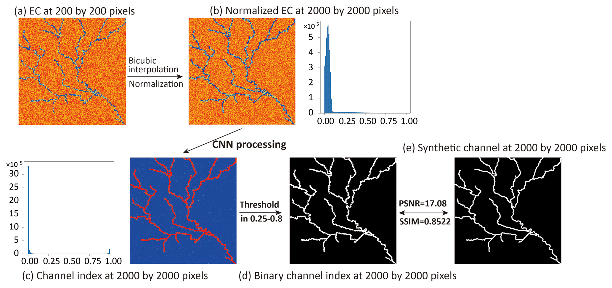
Figure 6 Workflow for generating a binary paleovalley map: (a) upscaling the 200×200 pixel electrical conductivity image to (b) a 2000×2000 pixel image using bicubic interpolation; (c) SRCNN processing; (d) generating a binary paleovalley at resolution of 2000×2000 pixels; (e) binary paleovalley with characteristics comparable to the original synthetic paleovalley.

It is worth noting that as the resolution of the resultant paleovalley increases, the PSNR and SSIM goodness-of-fit metrics and connectivity do not change significantly (Fig. 7). Both PSNR and SSIM increase with the resolution from 200×200 to 800×800 pixels because the bicubic interpolation smoothes the EC values and reduces the noise in EC values. When the image resolution further increases from 800 to 2000, PSNR degrades weakly from 18.48 to 17.09 (corresponding to an increase in mean-square error from 0.014 to 0.019) and, similarly, SSIM decreases from 0.8919 to 0.8522.

Because each image has a fixed extent of 80 m ×80 km, as the resolution increases, the distance between pixels and the real geological scale of 50×50 pixel images decreases. When the resolution increases from 200×200 to 2000×2000 pixels, the distance between pixels decreases from 400 to 40 m and the real scale of each training image decreases from 20 km ×20 km to 2 km ×2 km. When training the SRCNN, the distance between pixels was not accounted for. The training images in the training dataset include images without any paleovalley and images being fully occupied by the paleovalleys, with the narrowest paleovalley occupying merely 1 pixel. These paleovalley patterns are unrelated to the real scale of the training image, i.e., across the range from 20 km ×20 km to 2 km ×2 km. Thus, the trained SRCNN works well to infer paleovalleys across different resolutions and scales.

4.4 Application to APY lands AEM data

Following the training and testing of the SRCNN method based on synthetic DEM-derived paleovalley networks, we now apply the trained network to an area in the APY lands to convert EC values at a spatial resolution of 400 m ×400 m to identify paleovalleys at a resolution of 40 m ×40 m in an area of 80 km ×80 km. The methodology was first applied to a single depth AEM image (i.e., 100 m) to illustrate the procedure and discuss the main findings. In a second step we will apply the methodology to the AEM images from all 10 depths to extract specific information on the depth structure of the paleovalley network.

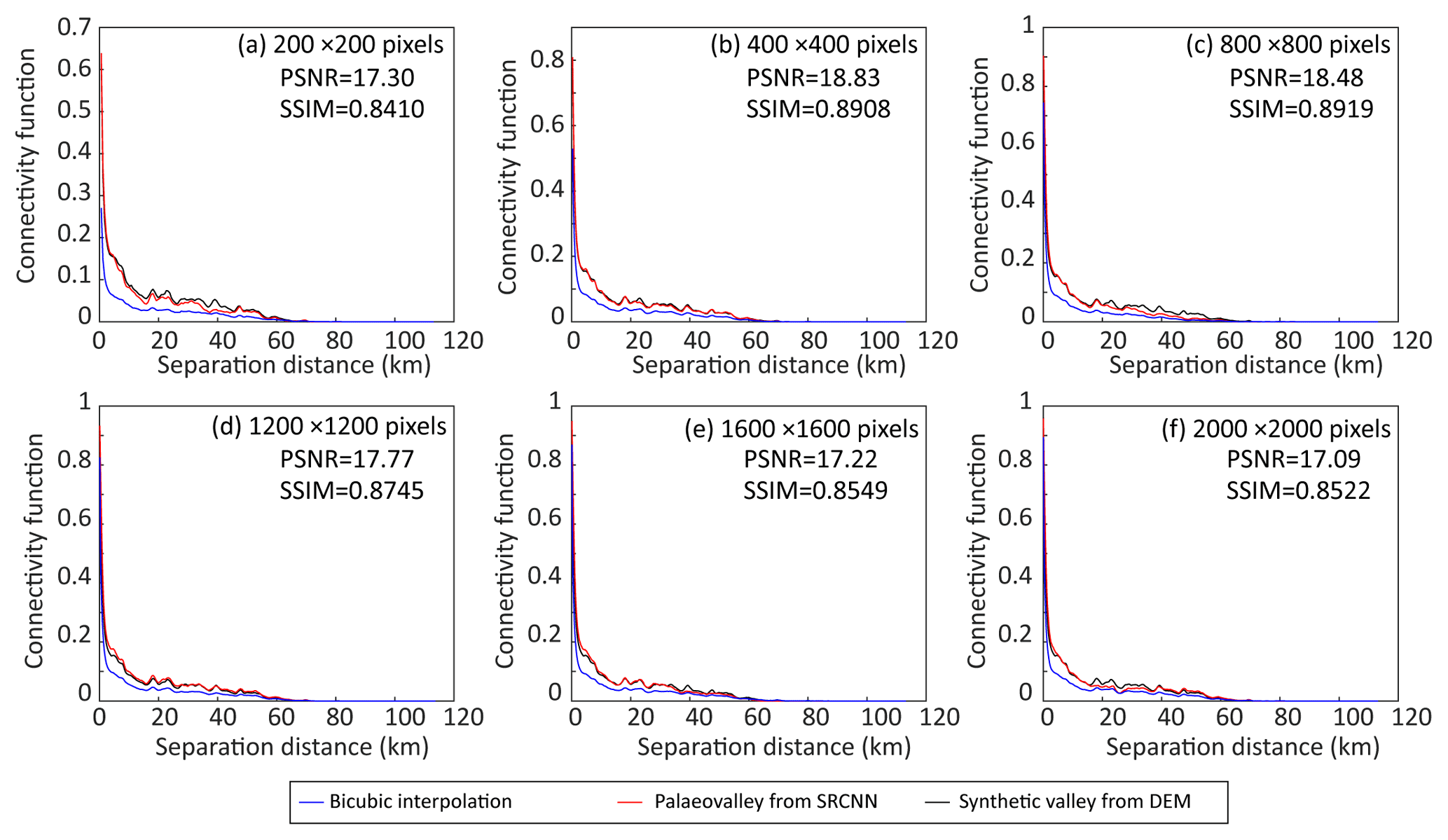
Figure 7 The PSNR, SSIM and connectivity of paleovalleys generated by SRCNN for different resolutions of upscaling the low-resolution EC image to a high-resolution binary paleovalley.

Figure 8 summarizes how the previously trained SRCNN successfully converts the low-resolution EC values resulting from an AEM survey to a binary map composed of paleovalleys and non-paleovalley areas (Fig. 8a). First, the bicubic interpolation generates a high-resolution EC image characterized by a right-skewed distribution of normalized EC values (Fig. 8b). This map does not yet allow a clear differentiation of the paleovalley from the surrounding fractured rocks. However, once we apply the SRCNN, a paleovalley index map with the paleovalley index following a binomial distribution is produced (Fig. 8c). Selecting an appropriate index (0.5 here) separates paleovalley from non-paleovalley pixels (Fig. 8d).

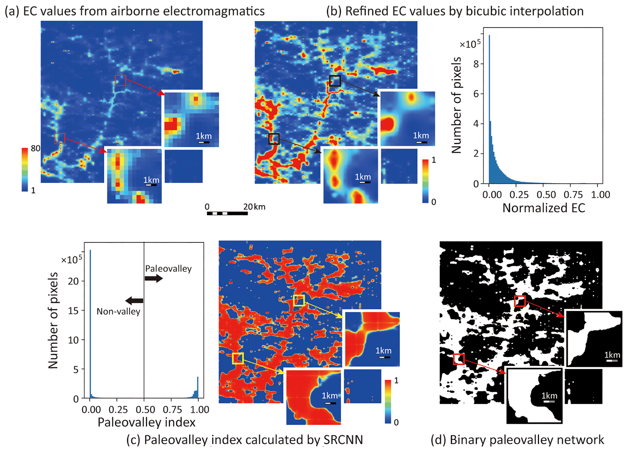
Figure 8 Steps to derive a binary paleovalley network in an 80 km ×80 km region in APY lands, Australia. (a) Raw EC map at a depth of 100 m; (b) EC map after bicubic interpolation; (c) paleovalley channel index map after application of the trained SRCNN method; (d) binary paleovalley map.

Inversion of AEM-derived EC maps at 10 depths within the first 100 m below the land surface (at 10 m intervals) is shown in Fig. 9a. EC values available at 10 layers are converted to binary paleovalley images by SRCNN, based on the premise that both the paleovalley pattern and bulk electrical conductivity from the 100 m depth interval can be represented in training images. As shown in Fig. 9a, normalized EC values derived from the AEM survey are characterized by a right-skewed distribution. However, once we apply the SRCNN, the resulting paleovalley index map (Fig. 9b) displays a binomial distribution of paleovalley indices. Selecting an appropriate index (0.5 here) generates a regional-scale 3-D binary paleovalley image with a horizontal resolution of 40 m and vertical resolution of 10 m (Fig. 9c).

Figure 9 (a) Rescaled AEM-derived EC map and corresponding histogram of normalized EC values within the depth interval of 100 m in an 80 km ×80 km region in APY lands, Australia; (b) paleovalley indices map and corresponding histogram after application of the trained SRCNN; (c) binary paleovalley map.

In the subsequent discussion we first test the derived paleovalley map with independent, yet limited, borehole data and auxiliary land surface maps. Next we extract further information from Fig. 9c about the depth structure of the paleovalleys to better constrain the areas for groundwater prospection.

To compare the paleovalley map (Fig. 9c) with borehole logs and an alternative indictor of the location of valley in the land surface (i.e., the multiple resolution valley bottom flatness index; Gallant and Dowling, 2003), we aggregated the 10 depth slices of Fig. 9c into a 2-D paleovalley index map, with values ranging from zero (i.e., no paleovalley within the 10 depth layers) to 10 (i.e., paleovalley detected across all depth layers) (Fig. 10a).

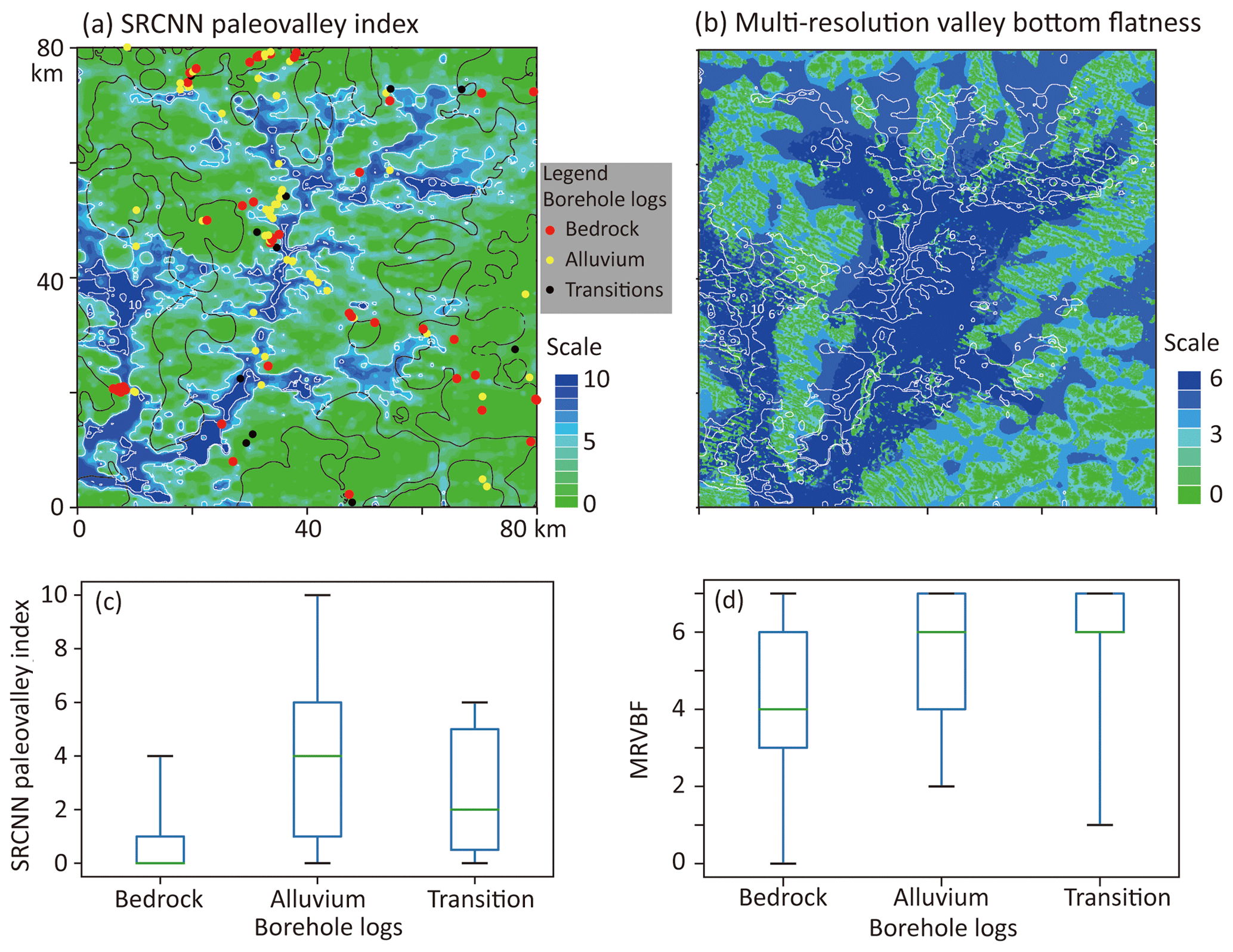
Figure 10 (a) SRCNN paleovalley index by aggregating the binary paleovalley in the vertical direction within 100 m; (b) multiple resolution valley bottom flatness (MRVBF) indicating the position of alluvium sediment accumulation. The black lines show the boundary between paleovalley and non-paleovalley interpreted from (b), while the white lines represent the contour lines of SRCNN paleovalley index from (a). The boxplot of SRCNN paleovalley index (c) and MRVBF (d) with respect to the borehole logs showing bedrock, alluvium and transition between bedrock and alluvium.

The resulting paleovalley index map in Fig. 10a is first compared to the Multiple Resolution Valley Bottom Flatness (MRVBF) index in Fig. 10b, which was originally calculated by Gallant and Dowling (2003) based on a digital elevation model with a spatial resolution of 100 m. High MRVBF values indicate a high probability of deposition of alluvium sediments. It was used by Munday et al. (2013), together with field observations of regolith, to obtain a hydrofacies map (black line in Fig. 10a). A comparison of the contours of the SRCNN paleovalley index 10 and 6 with the MRVBF index shows the emergence of similar patterns (Fig. 10a and b). While this confirms that the SRCNN paleovalley index map is not inconsistent with the MRVBF index, the latter contains insufficient information for testing the paleovalley map.

The degree to which the MRVBF index can be used to identify the main three hydrofacies (bedrock, alluvium and transition material) is discussed on the basis of Fig. 10d. High MRVBF values correspond to bores with both alluvial lithology and transition material lithology, while a large number of bedrock boreholes also show high MRVBF values. In other words, the alluvial (i.e., paleovalley) and bedrock/transition material (non-paleovalley) lithology classes could not be fully identified by the MRVBF index.

In contrast, the AEM survey and the paleovalley classification based on automatic neural networks in this study have improved our capability of identifying the position of paleovalleys. The boxplot of Fig. 10c shows that the boreholes classified as “alluvium” correspond to a higher median SRCNN paleovalley index of 4, compared to the two other lithology classes of median paleovalley index of 0 and 2, respectively. For 128 boreholes identified in the study area, (i) those drilled in bedrock (66 boreholes) had the smallest SRCNN paleovalley index (median of 0), (ii) those drilled in alluvium (57 boreholes) had the largest SRCNN index (median of 4) and (iii) those drilled in transition zones (five boreholes) had the next largest SRCNN index (median of 2). Despite the relatively small dataset of borehole logs (three per 100 km²), there is a clear trend that bores in alluvial sediments correspond to the areas with the highest SRCNN index. It is reasonable to assume that these alluvial sediments represent paleovalleys, although the lithological classification did not provide this level of detail. However, for 11 alluvial boreholes, only a low corresponding paleovalley index of < 2 was identified. This may be due to the limited lithological and sedimentary information captured by the downhole logs, which were mainly recorded in the 1970s with limited description of the subsurface environment. The same is true for the boreholes in bedrock and transition zones, which may have been misclassified due to insufficient data.

The paleovalley network shown in Fig. 10a is based on an analysis of 10 depth layers and hence gives greater confidence about the location of deep paleovalleys than the analysis of a single-depth paleovalley map (Fig. 8). A significant proportion of the image has a maximum index of 10, meaning that a paleovalley has been detected throughout the full investigation depth. This is thus an area with a high certainty (i.e., all pixels with index 10 have 10 layers identified as paleovalley) that at least a 100 m deep paleovalley is present. For the subsequent indices, e.g., 8, 6 and 4, at least eight, six and four depth layers with a paleovalley were identified, respectively.

Moreover, the burial depth of the paleovalley (defined by the vertical distance between the uppermost parts of the paleovalley to the land surface) is calculated based on the 3-D binary paleovalley. It is shown in Fig. 11a that a wide range of the paleovalleys are buried up to a depth of 10 to 20 m, which cannot be observed directly from the land surface, but can be revealed by the methodology proposed in this work based on geophysical prospecting (here 3-D AEM data).

We finally calculate the thickness of paleovalley layers (potentially representing the thickness of an alluvium aquifer) from the 10 depth layers with paleovalley indices. As a result, the thickness of the paleovalley calculated by the distance between bottom (lowest part) and top (uppermost part) of the paleovalley (Fig. 11b) is identical to the paleovalley index (Fig. 10b) multiplied by the layer thickness of 10 m. This indicates that except for those pixels that were shown to have a 10 to 20 m cover of non-paleovalley sediments (see burial depth in Fig. 11a), all other pixels had uninterrupted paleovalley layers starting from the land surface. In those paleovalley zones without surface sediment cover, the SRCNN paleovalley indices 8, 6 and 4 of Fig. 10a are representative for uninterrupted paleovalley sediments in the depth intervals 0–80, 0–60 and 0–40 m, respectively.

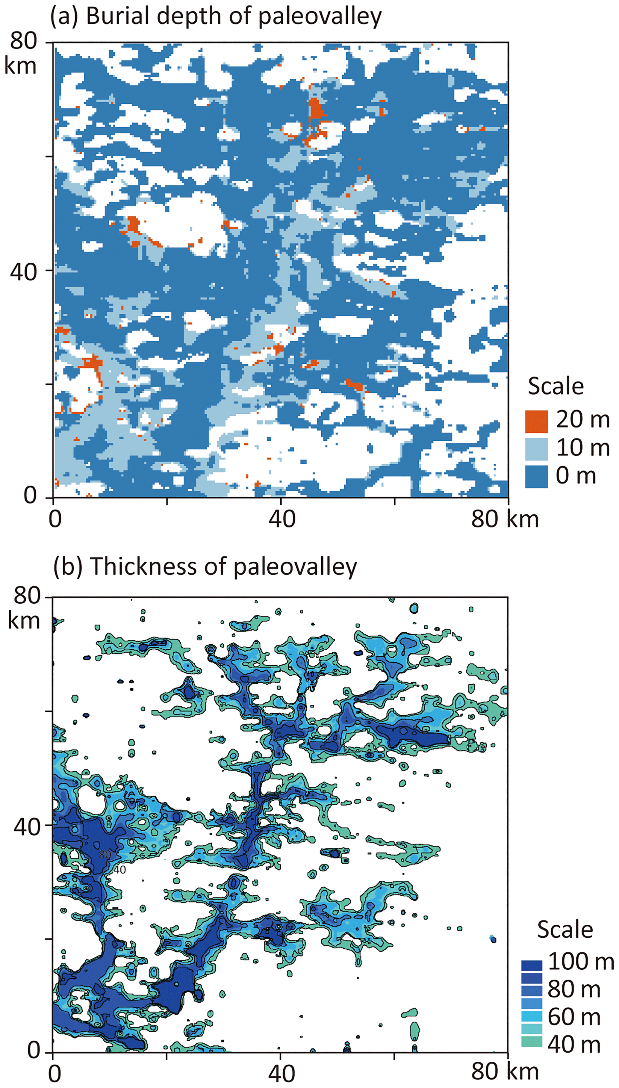
Figure 11 (a) Burial depth and thickness (> 40 m) of the alluvium sediments in paleovalleys inferred from the 3-D binary valley image of Fig. 9c with a 10 m vertical resolution. The hollow zone in (a) represents no identified paleovalleys within the depth of 100 m in the study area.

Note that in Fig. 10a at any pixel with given paleovalley index n (from 0 to 10), the probability of finding n consecutive paleovalley layers can be inferred; in our test case area this was 100 % everywhere – except for the buried pixels with 10 to 20 m cover of non-paleovalley sediments – as no interruption was detected in the sequence of paleovalley layers identified. This demonstrates that despite expected vertical lithological heterogeneities within paleovalleys (Knight et al., 2018), AEM images combined with our SRCNN methodology are able to identify and differentiate a broad series of sediments that make up a paleovalley from the surrounding bedrock. The SRCNN paleovalley index map thus provides an improved tool for groundwater prospectivity.

5 Conclusions

The super-resolution convolutional neural network (SRCNN) approach is one of many deep learning methods developed recently to sharpen image quality and to extract particular features from images. This study was one of the first SRCNN approaches to resolve a long-standing challenge in the earth sciences: how to generate high-resolution binary paleovalley maps from low-resolution electrical conductivity data derived from airborne electromagnetic surveys. The training images were generated using present-day valley patterns derived from DEM data as analogues to the paleovalley patterns at different depths, together with Archie's equation and bicubic interpolation to generate the corresponding electrical conductivity images. The large training image dataset featured the responses of airborne electromagnetics (AEM) data to the paleovalley system with noise. Following a supervised learning, SRCNN successfully removed noise from AEM-derived electrical conductivity (EC) data and classified EC values into two separate paleovalley index groups: one close to zero (the non-paleovalley areas) and another one near unity (the paleovalley areas). The resultant bimodal histogram of paleovalley index was then used to select threshold values to convert paleovalley indices to a binary paleovalley and non-paleovalley image. SRCNN can accommodate the spatial correlation between EC and paleovalley index by moving filters to recreate the connectivity of the paleovalley network. Moreover, the high-resolution of paleovalley patterns can be inferred from low-resolution EC images via SRCNN, as long as their relationship is addressed in the training image dataset.

However, there are several limitations to the method that require more work. In applying the SRCNN methodology, only EC images were used here to identify the paleovalley network. In those areas where paleovalley and non-paleovalley zones contain fluid with similar salinity, leading to similar bulk EC values, more geophysical information, e.g., gravity and magnetics, can be used as inputs in SRCNN to distinguish the position of the paleovalley. To generate a large training image pool, SRCNN was based on 2-D training images derived from DEM data. The trained SRCNNs were employed at different depth slices independently, where they were stacked up into a quasi-3-D paleovalley image. However, the vertical relationship between EC and paleovalley index could not be addressed. In the future, the 3-D paleovalley patterns in the training dataset could be generated by process-based methods (e.g., sedimentary processes modeling) or multiple geostatistical approaches, and 3-D images could be used in SRCNN to address horizontal and vertical correlations between EC and paleovalley index simultaneously. In addition, when applying the SRCNN methodology to a new study area, the training images need to be updated according to the factors influencing the relationship between target geobody and electrical conductivities (i.e., porosity, water content and sediment components in Archie's equation).

Appendix A: Robustness testing of the SRCNN methodology

The neural network settings used in this study were as follows: f₁=9, f₂=1 and f₃=5 and n₁=64, n₂=32 and n₃=1, where f represents the filter size and n represents number of output images from layer 1, layer 2 and layer 3, respectively, the size of input image is 50, and the overlapping size of EC values between paleovalley and non-paleovalley zone is 5 %. We now modify each of these parameters individually while fixing the others to investigate the robustness of the SRCNN as quantified by the performance metrics PSNR, SSIM and connectivity.

A1 Overlapping size

In this study, an overlap in EC values between paleovalley and non-paleovalley zones is induced to reflect impact by factors such as noise and smoothing in the AEM data interpretation and interpolation; the maximum overlapping size discussed is 5 % of the range of EC values (1–80 mS m⁻¹).

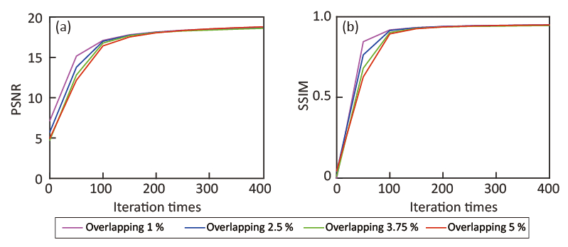
Figure A1 (a) PSNR and (b) SSIM calculated by SRCNN based on testing datasets in 400 iterations.

As shown in Fig. A1, the EC overlap between non-paleovalley and paleovalley zones in the training dataset only alters the speed at which the metrics PSNR and SSIM stabilize, but it does not affect the final PSNR and SSIM values. When the overlap size in the training dataset is comparable to that in the testing dataset (i.e., 5 %), the SRCNN can be trained to generate images with a similar accuracy. Furthermore, a cross test in Fig. A2 illustrated that the trained SRCNN can identify the paleovalley in the testing dataset with an overlap size smaller than that of the training image. However, if a small overlap size was employed in the training dataset (e.g., overlap size of 1 %), the trained SRCNN failed to identify the paleovalley cells in the testing dataset that had a larger overlap size (e.g., 5 %).

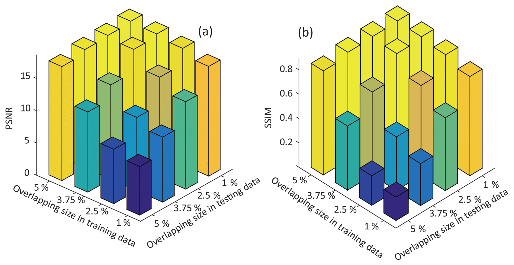
Figure A2 Effect of different degrees of EC overlap between paleovalley and non-paleovalley cells on model performance using (a) PSNR and (b) SSIM metrics.

This indicates that the SRCNN can be trained to remove noise in EC and identify the paleovalley cells based on training datasets, despite a certain degree of overlap in EC values between paleovalley and non-paleovalley. As a general rule, for the SRCNN to be successful, the overlap size in the training dataset should be larger than that in the testing dataset.

However, this does not mean that the larger degree of overlapping in a training dataset is always expected. As shown in Fig. A3, when compared to the synthetic paleovalley, the connectivity of paleovalleys resulting from SRCNN decays with the increase in the degree of overlapping in training dataset. This is because when a large degree of overlapping is contained in the training dataset, SRCNN considers more pixels with similar EC in both paleovalley and non-paleovalley zones as noise. After training, SRCNN removes too much noise and the resultant paleovalleys are disconnected (Fig. A3c). In contrast, when the degree of overlapping in the training dataset is low, the resulting image can contain noise in both paleovalley and non-paleovalley zones (Fig. A3b), but a better paleovalley connectivity is obtained. This suggests that although SRCNN can be trained to identify paleovalleys from EC images with a certain degree of overlapping, it is still desirable to constrain the degree of overlapping EC between paleovalley and non-paleovalley zones based on field data, e.g., the groundwater salinity, porosity and major minerals in rocks.

Moreover, the overlapping EC values here do not indicate that paleovalley and non-paleovalley cells have the same EC; otherwise, the AEM data will not contain enough information to separate the paleovalley and non-paleovalley zones. Furthermore, we need additional geophysical data, e.g., seismic velocity or gravity, to further constrain the paleovalley position. The inherent flexibility in the SRCNN methodology allows us to add more geophysical data, e.g., gravity and seismic velocity to the input image, to obtain an improved training of the relationship between the binary paleovalley image and multiple geophysical datasets. Demonstrating the information content of such datasets is beyond the scope of this paper.

A2 Input image size

The EC and binary paleovalley images with a size of 30×30 to 100×100 pixels are used to train the weights in the SRCNN. Although a larger input image size results in a higher PSNR metric, it does not significantly affect the SSIM metric (Fig. A4). Given the same number of iterations (6000) and batch size (50), the loss function is calculated at more pixels per iteration based on the larger input image. Consequently, longer computation times are required to train the SRCNN. Considering 6000 iterations takes merely 51 min to train the 30×30 pixel images, but 766 min is required to train the 100×100 pixel images (Fig. A5). Using large input images to train the SRCNN with fewer iterations has the same effects as using a small input image with more iterations.

However, as is evident from Fig. A5, the connectivity of SRCNN-generated paleovalleys decreases for input images of 30×30 pixels. This is because the correlation scale of EC and paleovalley index exceeds the input image size. In other words, the small-size training image limits the ability of SRCNN to address the spatial correlation of EC values and to recreate spatial connectivity. When the image size exceeds 50×50 pixels, the connectivity of generated paleovalleys corresponds well with the synthetic paleovalley. Further increasing the image size does not significantly affect the resultant paleovalley pattern.

A3 SRCNN depth, width and filter size

A larger filter size and network depth means more weights to be updated in the network, which potentially enhances the ability of the SRCNN in reproducing the paleovalley and non-paleovalley feature at each pixel. However, there is no strict criterion to determine the number of weights that yield a successful SRCNN model. It is reasonable to select the number of weights (i.e., unknowns) close to the size of training datasets (i.e., 60 000 knowns). Fewer weights could limit the capability of the SRCNN, while too many weights could cause overfitting risks in the SRCNN.

In the three-layer network with a filter size of 5-1-5, and output images of 64-32-1, the number of weights is 6592. When the filter size in the first layer increases to 9 and the depth of the network increases to 5, the number of weights becomes 59 328. Both are fewer than the size of the training dataset (60 000). While the increase in filter size and depths of SRCNN yield slightly higher PSNR and SSIM (Figs. A6 and A7), the drawback is that longer computation times are required (Fig. A7). With the total number of weights getting close to the size of the training dataset, the rate at which PSNR improves with increasing network depth slows down (Fig. A6). Conversely, a too deep network may remove too much noise from the paleovalley part, which makes the paleovalleys disconnected and the connectivity of the calculated paleovalley (green line in Fig. A7) diverts from the reference (black line in Fig. A7).

The filter size determines the spatial correlation length of EC values accounted for. Since we increase the filter size in the second layer to 5, a peak in PSNR and SSIM values and connectivity function are obtained in the full-size synthetic test (Fig. A7), although the number of weights in the network structure of 9(64)-5(32)-5(1) is not the largest among the five networks discussed. This suggests that a larger filter size is desirable to better address the spatial correlation of the EC values for paleovalley cells. However, it is also noted that for the size of the output image to be the same as that of the input image, part of the filter covers the zone outside the input image, where EC values of zero are used. This may cause errors in paleovalley index calculation, which is referred to as edge effect and can increase with filter size.

The depth of the network can also increase the correlation scale that is accounted for; the degree of this influence is determined by the filter size in each layer. In contrast, the width of each layer is unrelated to the correlation scale of EC and paleovalleys; it merely alters the degree of nonlinearity of the network by affecting the number of weights.

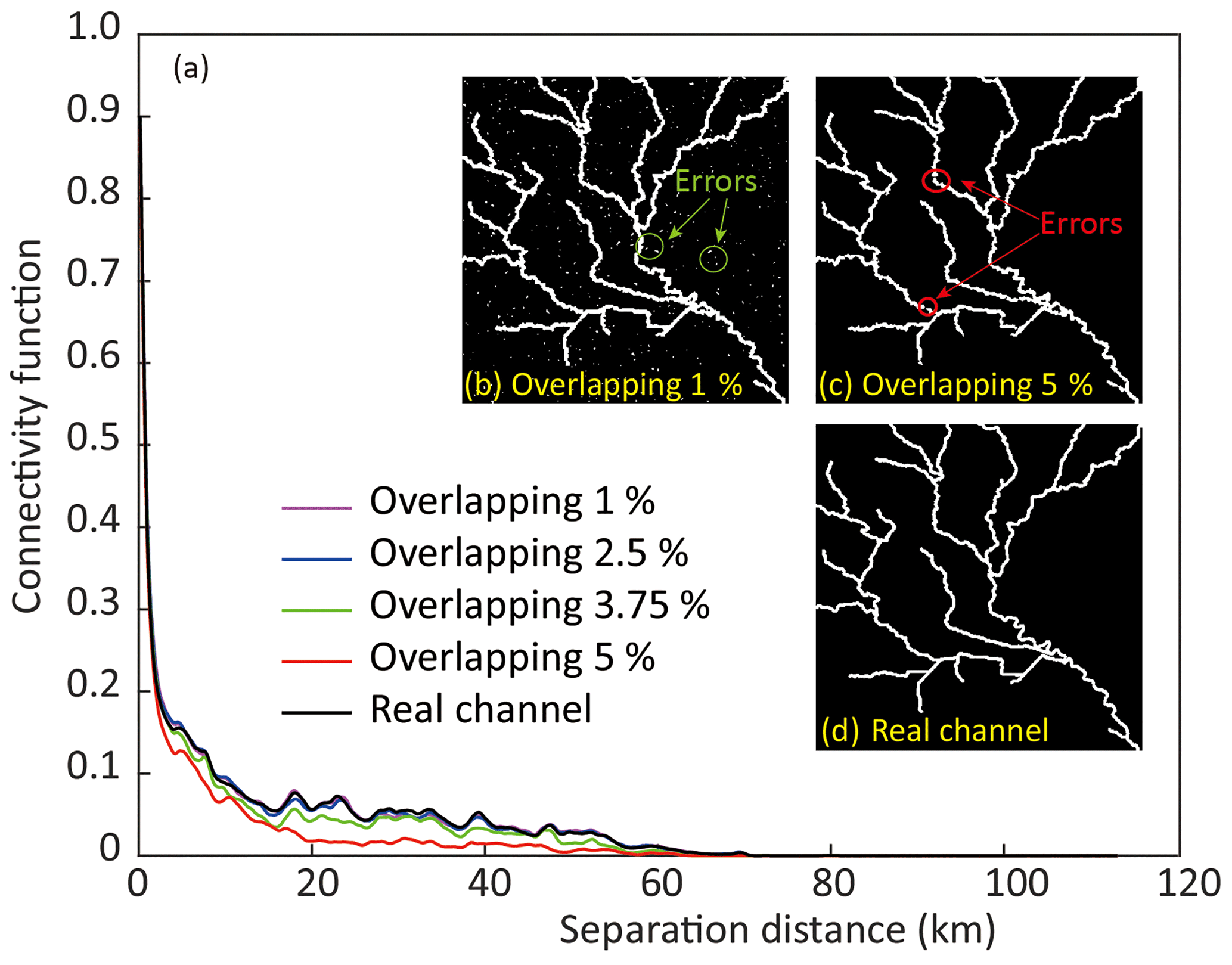
Figure A3 (a) Connectivity function in the northwest to southeast direction when applying the trained SRCNN to generate synthetic paleovalleys. Resultant paleovalley patterns using trained SRCNN with various degrees of overlap (1 % b and 5% c) in comparison with a real paleovalley (d).

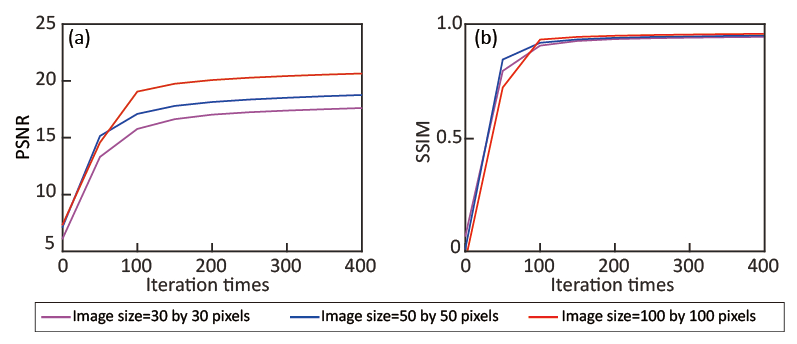
Figure A4 Performance criteria PSNR (a) and SSIM (b) calculated by the SRCNN for the testing dataset under varying input image sizes (30, 50 and 100).

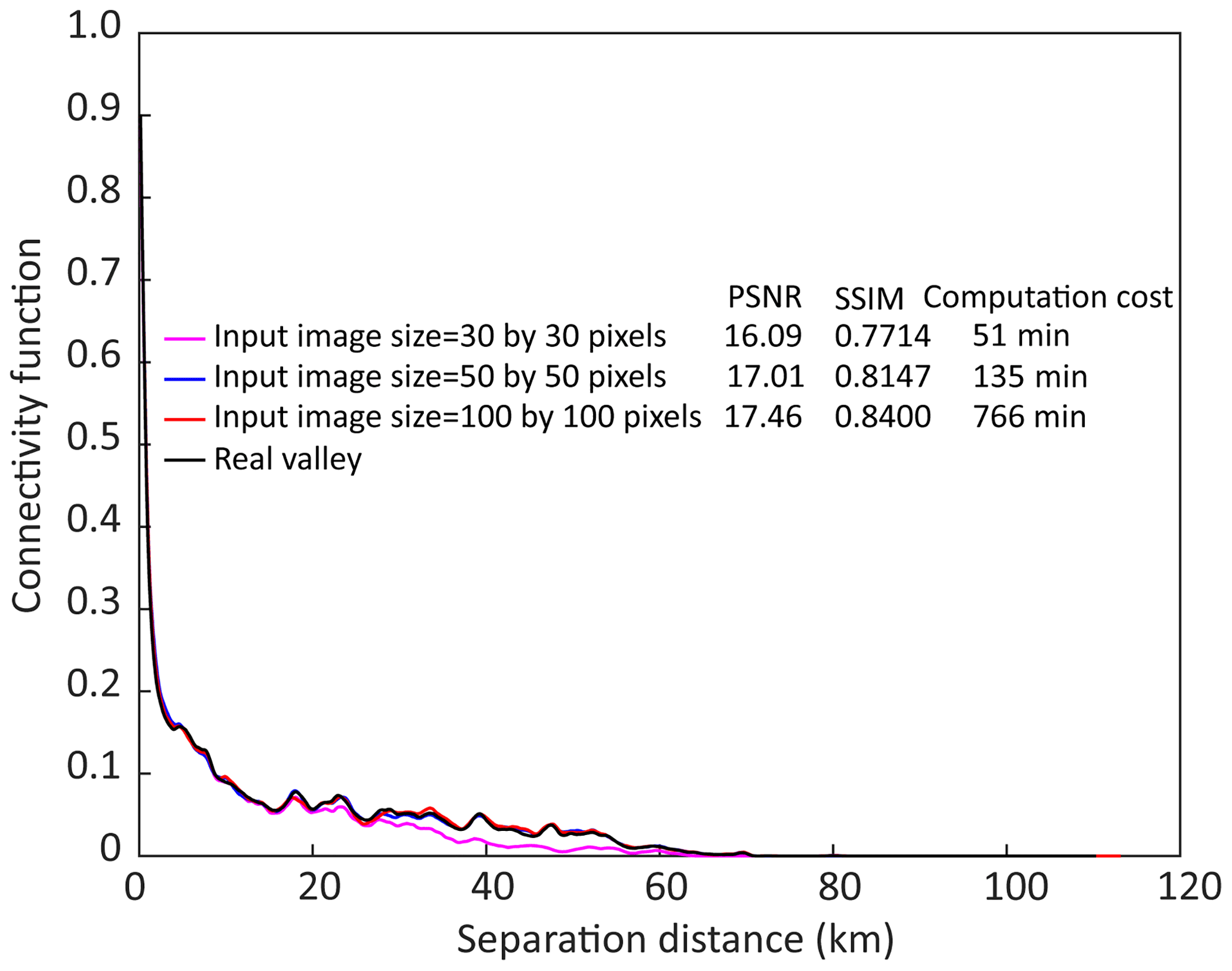
Figure A5 The connectivity function of the paleovalley generated by SRCNN, with the weight and bias values learned from the training images with sizes of 30, 50 and 100, respectively.

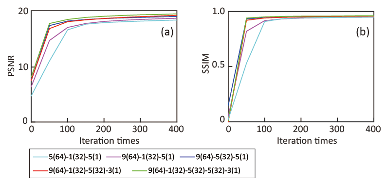
Figure A6 Model performance PSNR (a) and SSIM (b) calculated for the test dataset with varying SRCNN filter depths and filter sizes. Numbers are as follows: 5-1-5 in 5(64)-1(32)-5(1) represents the filter size in layers 1, 2 and 3, respectively, and (64)-(32)-(1) represents the number of output images of layers 1, 2 and 3.

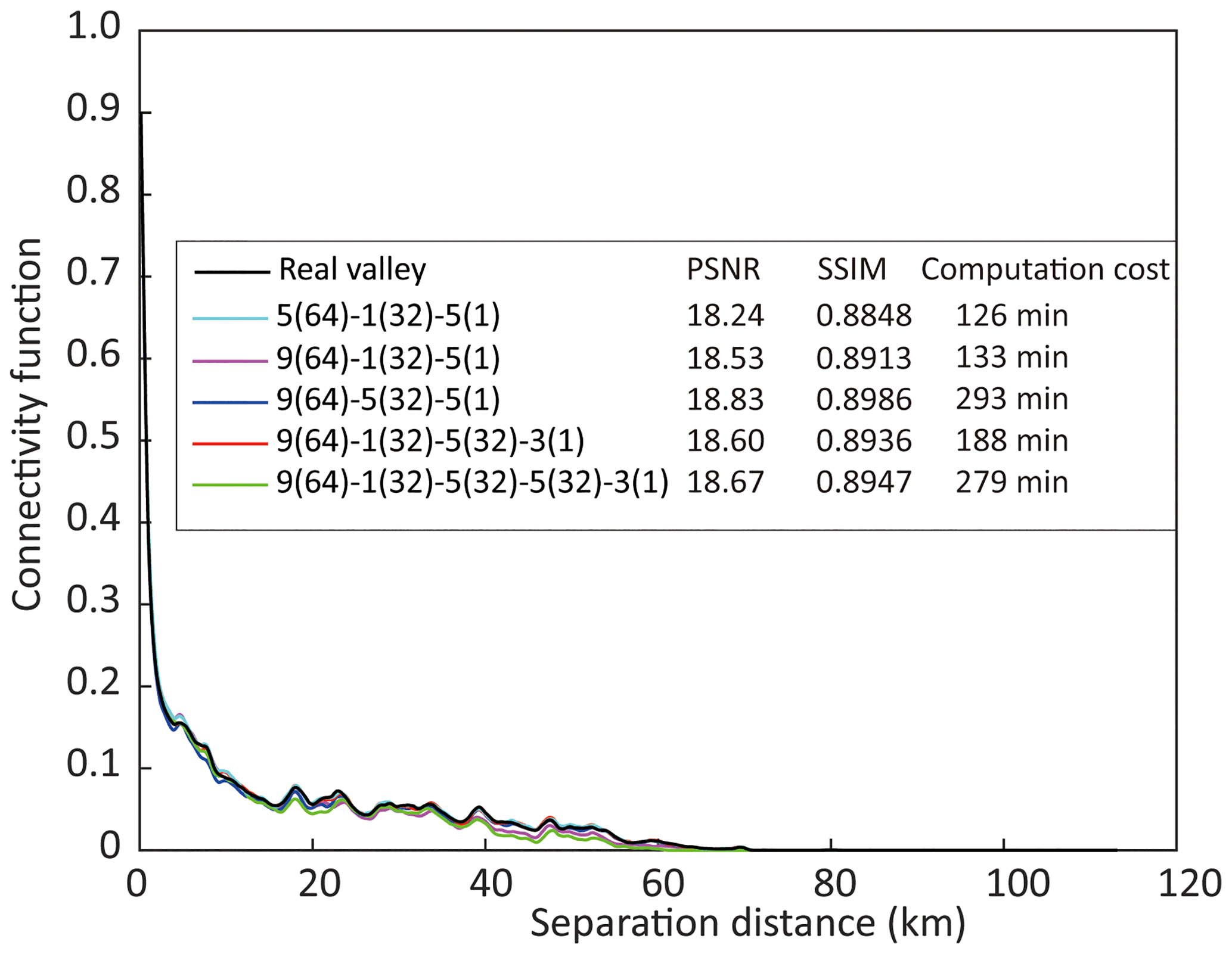
Figure A7 Connectivity of paleovalley generated by SRCNN with multiple depths and filter sizes. Computation cost is the time taken to train the SRCNN.