Multi-model approach to quantify groundwater-level prediction uncertainty using an ensemble of global climate models and multiple abstraction scenarios

Worldwide, groundwater resources are under a constant threat of overexploitation and pollution due to anthropogenic and climatic pressures. For sustainable management and policy making a reliable prediction of groundwater levels for different future scenarios is necessary. Uncertainties are present in these groundwater-level predictions and originate from greenhouse gas scenarios, climate models, conceptual hydro(geo)logical models (CHMs) and groundwater abstraction scenarios. The aim of this study is to quantify the individual uncertainty contributions using an ensemble of 2 greenhouse gas scenarios (representative concentration pathways 4.5 and 8.5), 22 global climate models, 15 alternative CHMs and 5 groundwater abstraction scenarios. This multi-model ensemble approach was applied to a drought-prone study area in Bangladesh. Findings of this study, firstly, point to the strong dependence of the groundwater levels on the CHMs considered. All groundwater abstraction scenarios showed a significant decrease in groundwater levels. If the current groundwater abstraction trend continues, the groundwater level is predicted to decline about 5 to 6 times faster for the future period 2026–2047 compared to the baseline period (1985–2006). Even with a 30 % lower groundwater abstraction rate, the mean monthly groundwater level would decrease by up to 14 m in the southwestern part of the study area. The groundwater abstraction in the northwestern part of Bangladesh has to decrease by 60 % of the current abstraction to ensure sustainable use of groundwater. Finally, the difference in abstraction scenarios was identified as the dominant uncertainty source. CHM uncertainty contributed about 23 % of total uncertainty. The alternative CHM uncertainty contribution is higher than the recharge scenario uncertainty contribution, including the greenhouse gas scenario and climate model uncertainty contributions. It is recommended that future groundwater-level prediction studies should use multi-model and multiple climate and abstraction scenarios.

1 Introduction

Groundwater is one of the major sources of high-quality freshwater across the world and one of the most important but scarce natural resources in many arid and semi-arid regions. However, these resources are under a constant threat of overexploitation and pollution all over the world due to anthropogenic and climatic pressure. Globally, groundwater provides 45 %–70 % of irrigation water (Döll et al., 2012; Shamsudduha et al., 2011; Taylor et al., 2013; Wada et al., 2013, 2014; Wisser et al., 2008), and the use of groundwater is continuously increasing. Overexploitation of groundwater for irrigation is worldwide one of the main causes of groundwater-level depletion (Mustafa et al., 2017b; Rodell et al., 2009; Scanlon et al., 2012; Wada et al., 2014). Climate change will probably also have an impact on the future availability of the groundwater resources (Brouyère et al., 2004; Chen et al., 2004; Goderniaux et al., 2009, 2011; van Roosmalen et al., 2009; Scibek et al., 2007; Taylor et al., 2013; Woldeamlak et al., 2007).

Food security of Bangladesh is highly dependent on sustainable use of groundwater for irrigation. However, in the northwestern part of Bangladesh, these resources are under a constant threat of overexploitation due to anthropogenic pressure. Mustafa et al. (2017b) report that overexploitation of groundwater for irrigation is the main cause of groundwater-level decline in the northwestern part of Bangladesh. In this context, the government of Bangladesh has plans to use more surface water instead of groundwater. However, the amount of groundwater that can be sustainably used for irrigation is still unknown. Also, the probable impact of shifting to more surface water use instead of groundwater is also unknown. Hence, research is needed to quantify the amount of groundwater that can be abstracted sustainably for irrigated agriculture in the northwestern part of Bangladesh.

Accurate predictions of groundwater systems, as well as sustainable water management practices, are essential for policy making. Transient numerical groundwater flow models are used to understand and forecast groundwater flow systems under anthropogenic and climatic influences. They provide primary information for decision-making and risk analysis. However, the reliability of groundwater model predictions is strongly influenced by uncertainties resulting from the model parameters, input data, and conceptual hydro(geo)logical model (CHM) structure (Refsgaard et al., 2006). Also, formulation of unknown future conditions, such as climatic change scenarios and groundwater abstraction strategies, increases the uncertainty in groundwater model predictions.

It is important to assess the different sources of uncertainty to ensure accurate prediction and reliable decision support in sustainable water resource management. The conventional treatment of uncertainty in groundwater modelling focuses on parameter uncertainty. Uncertainties due to model structure and due to scenario change are often neglected (Gaganis and Smith, 2006; Rojas et al., 2010). However, many researchers have recently acknowledged that the uncertainty arising from the CHM structure has a significant effect on model prediction (Neuman, 2003; Refsgaard et al., 2006). The incomplete and biased representation of the processes and the complex structure of a geological system often result in uncertainty in model prediction (Refsgaard et al., 2006; Rojas et al., 2008). Højberg and Refsgaard (2005) presented a case of a multi-aquifer system in Denmark by building three different CHMs using three alternative geological assumptions. They found that CHM structure uncertainty dominated over parameter uncertainty when the models were used for extrapolation. Many studies have recently suggested that uncertainty derived from the definition of alternative CHMs is one of the major sources of total uncertainty, and the parameter uncertainty does not cover the entire uncertainty range (Bredehoeft, 2005; Neuman, 2003; Refsgaard et al., 2006; Rojas et al., 2008; Troldborg et al., 2007). Therefore, neglecting the CHM uncertainty may result in unreliable prediction and underestimate the total predictive uncertainty.

Studies using a single CHM may fail to adequately sample the relevant space of plausible CHMs. Single model techniques are unable to account for errors in model output resulting from the structural deficiencies of the specific model. Rojas et al. (2010) noted that a CHM is assumed to be correct when the model is calibrated and validated successfully following an appropriate method as described by Hassan (2004a, b). However, a well-calibrated model does not always accurately predict the behaviour of the dynamic system (Van Straten and Keesman, 1991). Bredehoeft (2005) presented different examples where data collection and unforeseen elements challenged well-established CHMs. Choosing a single model out of equally important alternative models may contribute to either type I (reject true model) or type II (fail to reject false model) model errors (Li and Tsai, 2009; Neuman, 2003).

Although the concept of using alternative CHMs is increasingly applied among surface water modellers, in groundwater modelling the use of multi-model methods is limited. Recently, some studies have used multi-model methods in groundwater modelling to quantify the CHM uncertainty (Li and Tsai, 2009; Rojas et al., 2010). However, conceptual model uncertainty arising from the simplified representation of the hydro(geo)logic processes, geological stratification and/or boundary conditions has received less attention (Refsgaard et al., 2006; Rojas et al., 2010). Rojas et al. (2010) investigated uncertainty related to alternative CHM structures and recharge scenarios in groundwater modelling. However, the uncertainty arising from other sources such as general circulation models (GCMs), regional circulation models (RCMs), downscaling methods and abstraction scenarios in groundwater flow modelling still needs to be included in such approaches.

Climate change may significantly impact groundwater recharge. Recharge is one of the major input data in groundwater-level simulation. The future groundwater recharge is unknown, so it should be estimated based on different future climate scenarios. The GCMs project different climate scenarios based on the greenhouse gas emission scenarios (GHSs). The Special Report on the Emission Scenario, SRES (Nakicenovic et al., 2000), has reported different GHS emission scenarios. Besides, there are many GCMs to predict climate scenarios, and different GCMs use a different representation of the climate system (Flato et al., 2013; Gosling et al., 2011; Teklesadik et al., 2017). That means that different GCMs develop different climate projections for a single GHG emission scenario. Therefore, uncertainties arise in climate projections from GCMs and GHG emission scenarios. Another important source of uncertainties in climate projection is the internal variability of the climate system, i.e. the natural variability of the weather (Deser et al., 2012). Future climate change uncertainty arises from three main sources: external forcing, climate model response and internal variability (Hawkins and Sutton, 2009; Tebaldi and Knutti, 2007). Using an ensemble of climate scenarios has become common practice in analysis of climate change impact in the field of hydrology. Uncertainty analysis of groundwater simulations related to climate change has received relatively limited attention (Goderniaux et al., 2009; Taylor et al., 2013). Holman et al. (2012) recommended that climate scenarios from multiple GCMs or RCMs should be used to predict the impact of climate change on groundwater. Recently, several researchers have studied the impact of climate change on the groundwater system, incorporating uncertainty from the input of different GCM or RCM scenarios and different greenhouse gas emission scenarios (Ali et al., 2012; Dams et al., 2012; Jackson et al., 2011; Neukum and Azzam, 2012; Stoll et al., 2011; Sulis et al., 2012). The uncertainty analysis is, however, usually limited to the climatic part. Very recently, Goderniaux et al. (2015) included uncertainty related to model calibration in predicting groundwater flow along with uncertainty from the GCMs and RCMs and downscaling methods. However, the uncertainty arising from other sources, such as the model conceptualization and abstraction scenarios, is not evaluated.

Groundwater levels are often heavily influenced by the groundwater abstraction rate. For example, in the Indian subcontinent, groundwater abstraction has increased from 10–20 km³/year to approximately 260 km³/year during the last 50 years (Shamsudduha et al., 2011). In the northwestern part of Bangladesh, about 97 % of the total groundwater abstraction is used for irrigated agriculture (Mustafa et al., 2017b; Shahid, 2009). Shahid (2011) found an increasing trend in irrigation application rate in Boro rice, the major irrigated crop in the area. Details on current groundwater abstraction, trends in the abstraction and irrigated area can be found in Mustafa et al. (2017b). This increasing trend is ascribed to climate change. In contrast, improvement in agricultural water use efficiency can reduce the water use in irrigated agriculture. Therefore, multiple abstraction scenarios should be used to predict a reliable uncertainty band.

Existing literature on future groundwater-level prediction uncertainty quantification has focused on hydrological model calibration and climate model uncertainty considering one single CHM and parameter uncertainty. As far as the authors are aware, little research has been done so far to quantify future groundwater-level prediction uncertainty considering the uncertainty arising from the CHM structure, climate change and groundwater abstraction scenarios. This is the first attempt to evaluate the combined effect of CHM structure and the climate change and groundwater abstraction scenarios on future groundwater-level prediction uncertainty.

The general objective of this study is to quantify groundwater-level prediction uncertainty in climate change impact studies using a multi-model ensemble, i.e. an ensemble of representative concentration pathways, global climate models, multiple alternative CHMs and abstraction scenarios to provide probabilistic and informative predictions of groundwater levels. The specific objectives to achieve the general goal of this study are to (i) quantify the groundwater-level prediction uncertainties arising from the definition of alternative CHMs; (ii) analyse the effect of climate change on the groundwater levels using ensemble global climate models and estimate the uncertainty linked to climate scenarios; (iii) analyse the effect of groundwater abstraction scenarios on the future groundwater levels; (iv) quantify the amount of water that can be abstracted sustainably for irrigated agriculture in the northwestern part of Bangladesh; (v) evaluate the combined effect of CHM structure and the climate change and groundwater abstraction scenarios on future groundwater-level prediction uncertainty; and (vi) compare the uncertainty arising from the alternative CHMs and climate scenarios and abstraction scenarios.

2 Methodology

2.1 Study area

The study area is located in the northwestern part of Bangladesh (Fig. 1a). The study area is a subtropical region with two distinct seasons: the dry winter season (November to April) and the rainy monsoon season (May to October). The average annual precipitation amount varies between 1400 and 1550 mm, but is not uniformly distributed over the year (Fig. S2 in the Supplement). Almost 83 % of the total annual amount occurs in the monsoon season. The average temperature varies between 25–35 ^∘C for March to June and 9–15 ^∘C for November to February. Groundwater depth in the study area is continuously increasing (Fig. S3). The study area consists of six northwestern districts (Rajshahi, Naogaon, C'Nawabganj, Joypurhat, Bogra and Nator) and covers about 7112 km². In comparison to other districts of Bangladesh, these districts are more affected by drought (Shahid and Behrawan, 2008). The study area is situated between latitude 24^∘19^′0^′′ to 25^∘12^′0^′′ N and longitude 88^∘6^′36^′′ to 89^∘31^′12^′′ E. The surface elevation in the study area varies from 11 to 40 m (Fig. S1). There is a mild gradient towards the southeastern corner, and this corner is close to a large wetland.

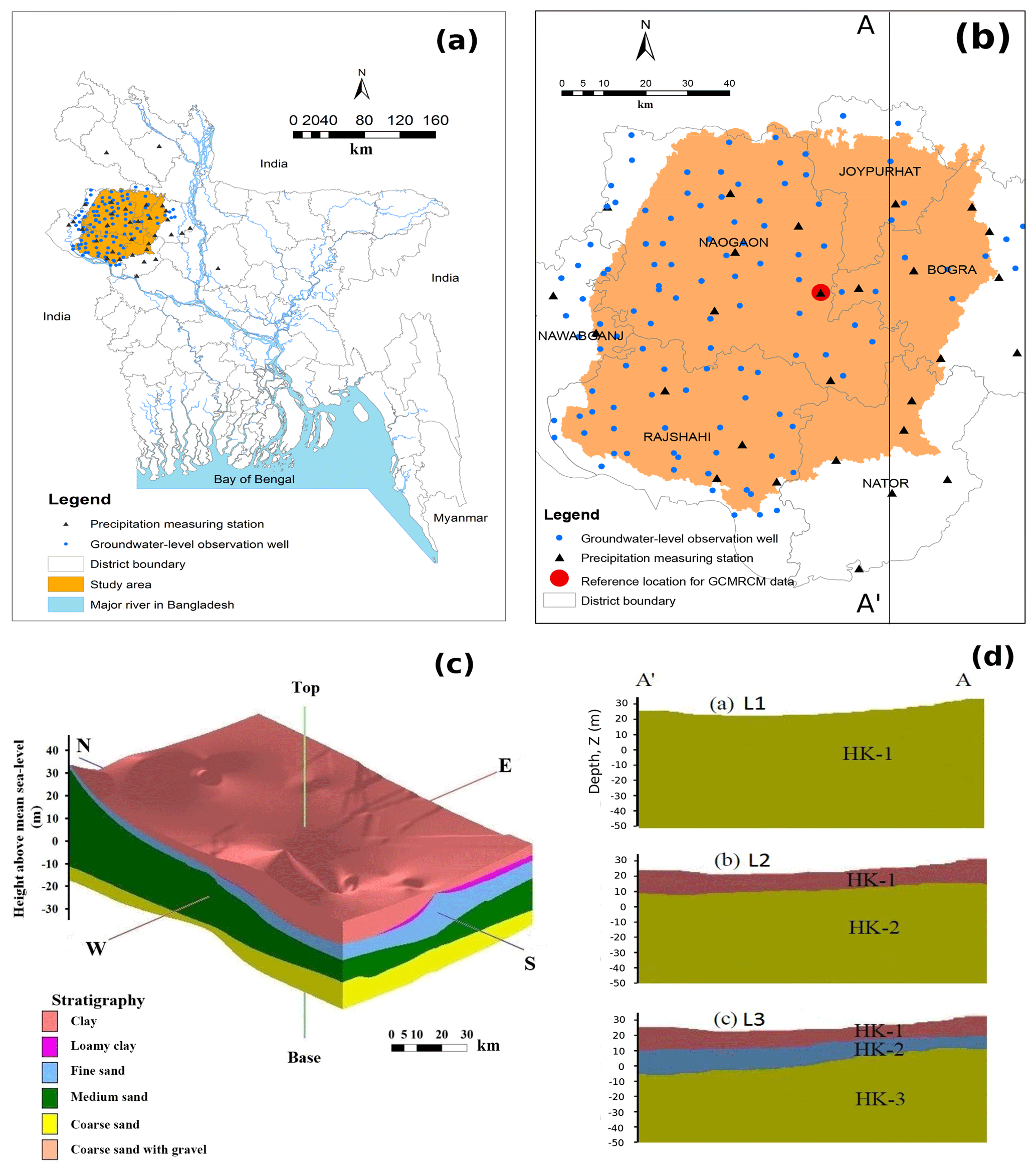
Figure 1 Description of the study area: (a) location of the study area in the northwestern part of Bangladesh; (b) study area with precipitation measurement stations (triangles) and groundwater observation wells (circles); (c) stratigraphy of the study area; (d) cross-sectional (A–A') view of different models: (a) one-layered model (L1), (b) two-layered model (L2), and (c) three-layered model (L3).

The aquifer in the study area is comprised of several layers such as clay, loamy clay, fine sand, medium sand, coarse sand and gravel with a dominance of medium to coarse sand (Fig. 1c). The thickness of each stratigraphic unit moreover varies spatially. The top layer consists of clay, clayey loam and fine sand with an average thickness of 18 m. It is underlain by a 20 m thick medium sand layer. Below the medium sand layer, a 35 m thick layer of coarse sand and coarse sand with gravel is present. The upper aquifer is unconfined or semi-confined with a thickness ranging from 10 to 40 m (Asad-uz-Zaman and Rushton, 2006; Faisal et al., 2005; Jahani and Ahmed, 1997; Michael and Voss, 2009b; Rahman and Shahid, 2004). The area is dominated by agriculture and almost 80 % is crop land. Irrigated agriculture plays an important role in the food production and security of Bangladesh, home to over 150 million people. In the northwestern part of Bangladesh irrigated agriculture is the major user of groundwater and accounts for 97 % of total groundwater abstraction (Shahid, 2009). Overexploitation of groundwater for irrigation, particularly during the dry season, causes groundwater-level decline in areas where abstraction is high and surface geology inhibits direct recharge to the underlying shallow aquifer (Mustafa et al., 2017b).

2.2 Data

Thirty-two years (1979–2011) of weekly groundwater-level and daily precipitation data of the Bangladesh Water Development Board (BWDB) and Bangladesh Meteorological Department (BMD) were collected from the Water Resources Planning Organization (WARPO), Bangladesh, for, respectively, 140 and 30 sites in the study area. Available river discharge data of the BWDB for the existing small rivers within the study area were also collected from WARPO. Daily minimum and maximum temperature, wind speed and other climatic data were collected from the BMD for all the available stations in the country. Reference evapotranspiration (ET₀), considered potential evapotranspiration in this study, was calculated using the FAO Penman–Monteith equation from the observed climatic data (Allen et al., 1998; Mustafa et al., 2017b).

The monthly observed groundwater head data of 50 observation wells were used for model calibration and validation and are plotted in a box-plot (Fig. S2). The groundwater levels vary between 3 and 22 m above mean sea level (a.m.s.l.) and display a clear seasonal variation. The groundwater level is relatively low in April and high in October.

The hydraulic properties of the aquifers were selected based on observed data and previous reports on the geology and lithology of the study area (Michael and Voss, 2009a, b). Topography and borehole data were collected from the Barind Multipurpose Development Authority (BMDA), Bangladesh. The log data from 23 boreholes within the study area were collected from the BMDA.

The climate model data are available through the website of the Earth System Grid Federation (https://esgf.llnl.gov, last access: 8 May 2019).

2.3 MODFLOW model

Processing MODFLOW or PMWIN (Chiang and Kinzelbach, 1998) is a physically based, fully distributed, grid-based, integrated simulation system for modelling groundwater flow and pollution. PMWIN was designed as a pre- and post-processor for groundwater flow model MODFLOW (Harbaugh and McDonald, 1996; McDonald and Harbaugh, 1988) to bring various codes together in a simulation system. The MODFLOW model is a physically based, fully distributed three-dimensional finite-difference numerical flow model developed by the U.S. Geological Survey (USGS). MODFLOW solves the three-dimensional partial-differential groundwater flow equation for porous media using a finite-difference method.

2.4 Multi-step multi-model methodology

A four-step methodology was used to achieve the objectives of the study (Fig. 2). In the first step, the climate model data for precipitation, minimum, mean and maximum temperature and ET₀ were extracted and downscaled as explained in Sect. 2.6. In the second step, monthly groundwater recharge was simulated using a spatially distributed water balance model (WetSpass) (Abdollahi et al., 2017; Batelaan and De Smedt, 2001) for the baseline period and for different scenarios as explained in Sects. 2.5.2 and 2.7. In the third step, 15 alternative conceptual hydrogeological models were constructed using different geological interpretations and boundary conditions. All alternative CHMs were calibrated using observed groundwater-level data. The performance of each model was evaluated based on different performance evaluation coefficients and information criterion statistics. The Bayesian model averaging (BMA) method was applied to obtain an average prediction from the alternative models. Also, the performance of alternative models was evaluated based on the maximum likelihood BMA weight of each model. The better-performing models among the alternative models were used to project groundwater levels under different climatic and abstraction scenarios. The averaged projection and its uncertainty were estimated using BMA of the ensemble of alternative CHMs. In the final step, climate change impact was assessed. The details of the different materials and methods of each step are described in the following sections.

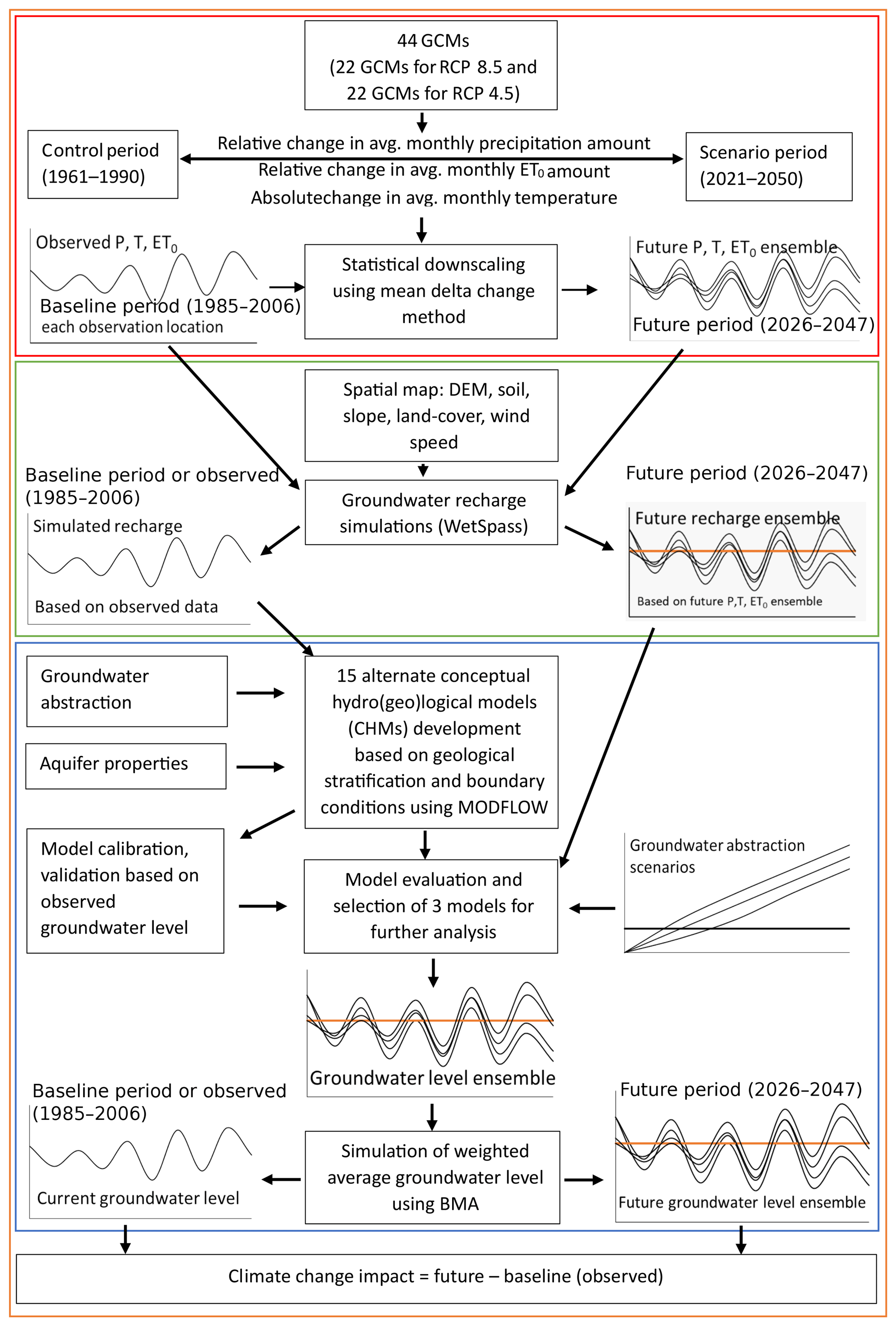
Figure 2 Multi-step multi-model methodology. GCM: general circulation model; RCP: representative concentration pathway; ET₀: potential evapotranspiration; P: precipitation; T: temperature; DEM: digital elevation model; BMA: Bayesian model averaging.

2.5 Alternative conceptual groundwater flow models

To estimate the uncertainty due to the conceptualization of groundwater models, 15 different alternative CHMs were developed based on geological stratification and boundary conditions. The cross-sectional (A–A') view of the models is shown in Fig. 1d. First, three simplified alternative conceptual groundwater models were defined based on the geological stratification. The three models are a one-layered (L1), two-layered (L2) and three-layered (L3) model. In the one-layered model (L1), the entire model domain was considered as one hydro-stratigraphic unit and the hydraulic properties are assumed homogeneous and isotropic. The two-layered model (L2) consists of two layers where the average thickness of the top layer was 10 m (clay and loamy clay soil) and the rest of the thickness was considered as the bottom layer. The model domain was divided into three different hydro-stratigraphic units to develop a three-layered model (L3). Below the top layer, a fine sand layer with an average thickness of 8 m was added in the three-layered model. The bottom layer of the three-layered model consists of medium sand, coarse sand and coarse sand with gravel.

Boundary conditions strongly influence the CHM uncertainty (Wu and Zeng, 2013). They are often very uncertain, and, moreover, strongly influence the model results. Previous studies in the Bengal Basin (Michael and Voss, 2009a, b) identified a north-to-south groundwater flow direction. On the other hand, there is a large wetland at the southeastern corner of the study area as well as a large river (known as Ganges/Padma) within a few kilometres of the southern boundary. Since exact boundary conditions were not known, based on the above information, five different potential sets of boundary conditions were conceptualized and shown in Fig. 3. For boundary condition B1, a no-flow boundary condition was assumed on every side of the model. In other words, there is no interaction between the model domain and the environment (Michael and Voss, 2009a, b). For boundary condition B2, a constant head boundary is assumed at the northern side where most of the river branches originated, assuming that groundwater flow direction is parallel to the river flow and perpendicular to the model boundary. No-flow boundary conditions were assumed for all other sides. For boundary condition B3, a constant head boundary was considered on the northern side like for B2 and the southeastern side, i.e. the side where a large wetland is located. Boundary condition B4 is based on boundary condition B3. The constant head boundary in the southeastern part of the model was extended to the southern part of the model domain in boundary condition B4 because the great Ganges/Padma River is very near to the southern boundary. In boundary condition B5, a constant head boundary was considered at the northern and northwestern boundary and also at the southeastern corner of the model domain based on the information that groundwater is flowing from north and northwest to south (Michael and Voss, 2009a, b). A constant head is assigned at the southeastern corner of the model domain representing the Chalan Beel wetland as well. No-flow boundaries are assumed at the southern and northeastern boundaries since these boundaries are parallel to the groundwater flow direction (Michael and Voss, 2009a, b). The long-term monthly average groundwater levels (normal) were considered as the constant groundwater heads for the constant head boundary. As there is seasonal variability in the groundwater level of this study area, every month was assigned a different constant groundwater head corresponding to the long-term average groundwater level for that month.

In total, 15 alternative groundwater models were developed using 5 different boundary conditions and 3 different layer types. A list of the 15 models is included in Table S1.

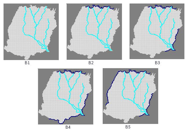
Figure 3 Boundary conditions used to develop alternative conceptual models (dark blue line indicates a constant head boundary). B1: no-flow boundary; B2: constant head at the northern boundary; B3: constant head at the northern and southeastern boundaries; B4: constant head at the northern, southern and southeastern boundaries; B5: constant head at the northern, northwestern and southeastern boundaries.

2.5.1 Model setup

The BIock Centered Flow Package (BCF) of MODFLOW-96 within the PMWIN interface was used for groundwater flow simulation. The study area covers an area of 7112 km² discretized into smaller cells with 117 rows and 118 columns. The grid cell dimension is 900 m ×900 m. All models are transient with a monthly time step. A no-flow boundary is considered at the model domain bottom as the vertical groundwater flow is restricted by the relatively impermeable hard rock below the aquifer in the study area. On the model top surface, a spatially distributed recharge boundary is considered.

The initial groundwater heads correspond to a long-term average groundwater table obtained by running the models in steady-state conditions.

The range of hydrogeological parameter values was selected based on typical values for aquifer materials (Domenico and Mifflin, 1965; Domenico and Schwartz, 1998; Johnson, 1967) and previous research findings in the study area (Michael and Voss, 2009a, b). They are listed in the Supplement. Michael and Voss (2009a) used $\mathrm{9.4}\times {\mathrm{10}}^{-\mathrm{5}}$ m⁻¹ as a specific storage value for the Bengal Basin. The initial specific storage was taken as $\mathrm{9.4}\times {\mathrm{10}}^{-\mathrm{5}}$ m⁻¹ when it is within the specific storage limits of the aquifer materials according to the literature. Otherwise, the initial specific storage was taken as the average of the maximum and minimum values of the aquifer materials found in the literature. The rivers in the study area are typically small and mainly driven by precipitation runoff. Generally, there is no flow in the rivers during dry months (January to March). The “River flow package” of MODFLOW was used to define rivers in the model domain and a third-type boundary condition was assumed for the rivers. Riverbed conductance is indeed defined as a lumped parameter in MODFLOW defined as

$$\begin{array}{}\text{(1)}& {\displaystyle }\mathrm{CRIV}={\displaystyle \frac{K_{\mathrm{riv}}\times L\times W}{M_{\mathrm{riv}}}},\end{array}$$

where CRIV is riverbed hydraulic conductance (L²T⁻¹), K_riv is riverbed sediment hydraulic conductivity (LT⁻¹), L is length of the river within a grid cell (L), W is width of the river within a grid cell (L) and M_riv is thickness of the riverbed within a grid cell (L).

From the equation, it is clear that riverbed hydraulic conductance depends on grid size, riverbed sediment hydraulic conductivity and thickness of the riverbed. Mehl and Hill (2010) have reported that riverbed conductance depends heavily on the grid size of the model. Due to a lack of field data for riverbed materials, the riverbed conductance was obtained through manual calibration: riverbed conductance is 0.18 m² s⁻¹, while riverbed thickness is 0.5 m.

2.5.2 Simulation of spatially distributed groundwater recharge

Spatially distributed monthly groundwater recharge was simulated using the WetSpass-M model (Abdollahi et al., 2017; Batelaan and De Smedt, 2001) on the same grid as the groundwater flow (MODFLOW) model. WetSpass-M is a physically based distributed model, in which the groundwater recharge is estimated from a grid-based water balance. To allow land cover heterogeneity within each cell, every raster cell is split into four fractions: vegetated, bare-soil, open-water and impervious. The water balances of each fraction are used to calculate the total water balance of a raster cell, whereas recharge is calculated as the residual term of the water balance for each cell. The inputs of the model are spatially distributed maps of land cover, soil texture, topography, groundwater depth and climatic data. Precipitation (including of rainy days), ET₀, temperature and wind speed were used as climatic information. Details on model setup and data preparation for groundwater recharge calculation data can be found in Mustafa et al. (2017b). Monthly groundwater recharge was simulated for 22 years (1985–2006) and considered the baseline groundwater recharge.

2.5.3 Groundwater abstraction estimation

Groundwater abstraction for irrigation was calculated from the available data. Unfortunately, detailed groundwater abstraction information, e.g. amounts of water pumped from individual wells, co-ordinates of the abstraction wells, capacity of the pumps or duration of pumping, were not available. Hence, the groundwater abstraction was assessed based on the irrigated area by shallow tube wells (STWs), deep tube wells (DTWs) and other irrigation equipment. Upazila-wise (an upazila is the second lowest tier of regional administration in Bangladesh) yearly seasonal groundwater abstraction for irrigation from the groundwater was calculated using an empirical equation based on Boro rice irrigation requirements and the irrigated area. The irrigation water withdrawal was considered to be the total abstraction for each upazila. To obtain monthly abstraction for each upazila, the calculated seasonal abstraction values are initially equally divided over the months of the dry seasons (November to April). Also, as the location of the pumps is unknown, the total abstraction from each upazila is initially considered uniformly distributed over the full upazila. Considering the individual upazila as 1 zone of abstraction, a total of 34 abstraction zones were considered. Details on the irrigation data can be found in Mustafa et al. (2017b) and Shamsudduha et al. (2015).

2.5.4 Calibration and validation of alternative CHMs

All alternative CHMs were calibrated for the period 1990–1994. Model parameters were estimated using manual calibration and automatic calibration. During auto-calibration, PEST (Doherty, 1994) was used to optimize the model parameter values.

The initial values, allowable ranges and optimized values of the parameters of the different models are given in the Supplement (Tables S2, S3, S4). One-layered-type models were calibrated for three parameters: horizontal hydraulic conductivity, specific storage and specific yield. The two-layered and three-layered models were calibrated for, respectively, 8 and 12 parameters. The process of selecting initial values and the allowable range of the different parameters is described in Sect. 2.5.1. The optimized horizontal hydraulic conductivity of the one-layered models varies between $\mathrm{4.45}\times {\mathrm{10}}^{-\mathrm{3}}$ and $\mathrm{6.00}\times {\mathrm{10}}^{-\mathrm{3}}$ m s⁻¹. This high value of horizontal hydraulic conductivity corresponds to well-sorted coarse sand and gravel (Fetter, 2001). We consider these values to be realistic since a major portion of the aquifer consists of coarse sand and coarse sand with gravel. The average horizontal hydraulic conductivity of the Bengal Basin found by Michael and Voss (2009a) was also high ($\mathrm{5}\times {\mathrm{10}}^{-\mathrm{4}}$ m s⁻¹). They also reported that, based on the drill-log analysis, horizontal hydraulic conductivity of the Bengal Basin may vary from $\mathrm{6}\times {\mathrm{10}}^{-\mathrm{6}}$ to $\mathrm{3.00}\times {\mathrm{10}}^{-\mathrm{3}}$ m s⁻¹. The area of the Bengal Basin is about 2.8×10⁵ km², but the study area is only a small part of the Bengal Basin. Therefore, it is possible that the horizontal hydraulic conductivity is relatively higher in our study area. Bonsor et al. (2017) have also reported in their review that aquifer materials in the Bengal Basin are highly permeable. Mustafa et al. (2018) have also reported that the average horizontal hydraulic conductivity of this study area is high and around $\mathrm{2.5}\times {\mathrm{10}}^{-\mathrm{3}}$ and $\mathrm{4.5}\times {\mathrm{10}}^{-\mathrm{3}}$ m s⁻¹.

Additionally, spatial variability of horizontal hydraulic conductivity has not been considered in this study. We consider an average horizontal conductivity for all individual layers. This might be another reason for high horizontal hydraulic conductivity.

The optimized specific storage of the one-layered model with boundary condition-5 (L1B5) was $\mathrm{4.92}\times {\mathrm{10}}^{-\mathrm{5}}$ m⁻¹. Michael and Voss (2009a) also reported a similar specific storage value ($\mathrm{9.4}\times {\mathrm{10}}^{-\mathrm{5}}$ m⁻¹) for the Bengal Basin. However, different conceptual models suggest different specific storage values within the typical values for aquifer materials depending on the number of layers and boundary conditions (Tables S2, S3, S4).

The optimized value of specific yield varies between 0.17 and 0.35 for different conceptual models. The results are in line with previous findings of specific yield values in the area which indicate that specific yield in the study area varies between 0.08 and 0.32, with higher values in the southern part of the Barind area (Jahan et al., 1994; Mustafa et al., 2018). However, the optimized values of specific yield for some conceptual models are equal to the upper boundary of the pre-defined parameter range. This could be because of the simplified representation of hydrogeological layers and properties of the system defined in some of the conceptual models. However, even with different conceptual models, the optimized value of specific yield is equal to the upper boundary of the parameter range, indicating that the calibrated values of the specific yield could not reach the real optimum. This could be because of uncertain groundwater abstraction and recharge data in this study area. Mustafa et al. (2018) have proven that groundwater abstraction and groundwater recharge data in space and time in this study area are highly uncertain. They have also reported that input uncertainty (uncertainties arising from groundwater abstraction and recharge) has a significant impact on the specific yield values. However, in this study, uncertainty of the input data has not been considered. Additionally, spatial and seasonal variability of the groundwater abstraction has not been considered in this study. This might be another reason for the high specific yield value. Further improvement of model calibration would require additional and more reliable groundwater abstraction and groundwater recharge data, such as time series of pumping discharge from individual wells and exact locations of all abstraction wells.

Using the optimized parameters, each of the alternative CHMs was validated for the period of 1995 to 1999.

2.5.5 Model performance evaluation

The performance of alternative conceptual groundwater models (CHMs) was evaluated using information criteria, statistical indicators and graphical presentation of simulated groundwater levels. Root mean square error (RMSE) and Nash–Sutcliffe efficiency (NSE, Eq. 2) of the alternative CHMs were calculated using the formula reported by Moriasi et al. (2007). The notation of Mustafa et al. (2017a) has been followed.

$$\begin{array}{}\text{(2)}& {\displaystyle }\mathrm{NSE}=\mathrm{1}-{\displaystyle \frac{{\sum }_{i=\mathrm{1}}^n(O_i-S_i{)}^{\mathrm{2}}}{{\sum }_{i=\mathrm{1}}^n(O_i-\stackrel{\mathrm{‾}}{O}{)}^{\mathrm{2}}}}\end{array}$$

Here, O_i and S_i represent observed and simulated values, respectively, $\stackrel{\mathrm{‾}}{O}$ is the mean of O_i and n is the number of observations.

NSE varies from −α to +1 and is dimensionless. NSE values closer to 1 mean better simulation efficiency. NSE values >0.7, 0.35–0.7, 0.0–0.35 and <0.0 represent, respectively, excellent, good, fair and poor performance.

Information criteria are often used for model ranking (Zhou and Herath, 2017). Different information criteria such as the Akaike information criterion (AIC), corrected Akaike information criterion (AICc), Kashyap information criterion (KIC) and Bayesian information criterion (BIC) were used to evaluate the alternative CHMs.

The Akaike information criterion is defined as (Zhou and Herath, 2017)

$$\begin{array}{}\text{(3)}& {\displaystyle }& {\displaystyle }\mathrm{AIC}=n\ln \left({\mathit{\sigma }}^{\mathrm{2}}\right)+\mathrm{2}p,\text{(4)}& {\displaystyle }& {\displaystyle }\mathrm{AICc}=n\ln \left({\mathit{\sigma }}^{\mathrm{2}}\right)+\mathrm{2}p+{\displaystyle \frac{\mathrm{2}p\left(p+\mathrm{1}\right)}{n-p-\mathrm{1}}},\text{(5)}& {\displaystyle }& {\displaystyle }{\mathit{\sigma }}^{\mathrm{2}}={\displaystyle \frac{\mathrm{SWSR}}{n}},\end{array}$$

where n is the number of observations (same for all models), p is the number of model parameters $=\mathrm{NPE}+\mathrm{1}$, NPE is the number of process model parameters and σ² is the residual variance. SWSR is the sum of weighted squared residuals.

The Bayesian information criterion (BIC) and Kashyap information criterion (KIC) are defined in Eqs. (6) and (7), respectively (Zhou and Herath, 2017):

$$\begin{array}{ll}\text{(6)}& {\displaystyle }& {\displaystyle }\mathrm{BIC}=n\ln \left({\mathit{\sigma }}^{\mathrm{2}}\right)+p\ln \left(n\right),{\displaystyle }& {\displaystyle }\mathrm{KIC}=\left(n-\left(p-\mathrm{1}\right)\right)\ln \left({\mathit{\sigma }}^{\mathrm{2}}\right)-\left(p-\mathrm{1}\right)\ln \left(\mathrm{2}\mathit{\pi }\right)\\ \text{(7)}& {\displaystyle }& {\displaystyle }+\ln \left|{\mathbf{X}}^T\mathit{\omega }\mathbf{X}\right|,\end{array}$$

where X is the sensitivity matrix (Jacobian matrix). The weighted factor ω applies when the errors are independent of each other.

The different information criterion values were obtained from MODFLOW by running PEST in sensitivity analysis mode. The best model among the alternative CHMs has a minimum information criterion value (minimum AIC or AICc or BIC or KIC) (Zhou and Herath, 2017). A posterior model probability (p_k) was calculated using Eq. (8) for each information criterion method for each alternative CHM. The posterior model probability was used to select the best CHMs. The better model corresponds to a larger posterior model probability (Zhou and Herath, 2017).

$$\begin{array}{}\text{(8)}& {\displaystyle }& {\displaystyle }{p}_k={\displaystyle \frac{e^{-\mathrm{0.5}{\mathrm{\Delta }}_k}}{{\sum }_{j=\mathrm{1}}^K{e}^{-\mathrm{0.5}{\mathrm{\Delta }}_j}}},\text{(9)}& {\displaystyle }& {\displaystyle }{\mathrm{\Delta }}_k={\mathrm{AIC}}_k-{\mathrm{AIC}}_{\min },\end{array}$$

where AIC_k is the AIC value for model k and AIC_min is the minimum AIC values of all models. The value of Δ_k was also calculated for AICc, BIC and KIC.

2.5.6 Bayesian model averaging

BMA was used to deduce more reliable predictions of groundwater levels than the predictions produced by the individual groundwater models. Draper (1995) and Hoeting et al. (1999) present an extensive overview of BMA. Recently, BMA has received attention of researchers of diverse fields because of its more reliable and accurate predictions than other model averaging methods. Vrugt (2016) has developed a model averaging MATLAB toolbox called MODELAVG for post-processing of forecast ensembles. The MODELAVG has different model averaging methods including BMA and was used in this study. Details of the model averaging method are described in the MODELAVG manual (Vrugt, 2016). The value of β_BMA (maximum likelihood Bayesian weight) was used as a criterion to select the better-performing models that have a significant contribution in model averaging.

The general equation used to calculate the weighted average prediction in various model averaging strategies is as follows:

$$\begin{array}{}\text{(10)}& {\stackrel{\mathrm{̃}}{y}}_j=\sum _{k=\mathrm{1}}^K{\mathit{\beta }}_k{D}_{jk},\end{array}$$

where D_jk is the bias-corrected point forecasts of each model, $k=\mathit{\{}\mathrm{1},\mathrm{\dots },K\mathit{\}}$ is model number and $j=\mathit{\{}\mathrm{1},\mathrm{\dots },n\mathit{\}}$ is forecast number, ${\stackrel{\mathrm{̃}}{y}}_j=\mathit{\{}{\stackrel{\mathrm{̃}}{y}}_{\mathrm{1}},\mathrm{\dots },{\stackrel{\mathrm{̃}}{y}}_n\mathit{\}}$ is the weighted average forecast for the jth forecast number, and $\mathit{\beta }=\mathit{\{}{\mathit{\beta }}_{\mathrm{1}},\mathrm{\dots },{\mathit{\beta }}_k\mathit{\}}$ denotes the weight vector.

2.6 Climate change scenarios

The climate model data for precipitation and minimum, mean and maximum temperature are extracted for the grid cells covering the reference location within the catchment. This reference location is set at 24.81^∘ N and 88.95^∘ E and is indicated by a red dot in Fig. 1b. Using the FAO Penman–Monteith equation based on the temperature from climate model data, ET₀ is calculated.

Within this case study, CMIP5 (Coupled Model Intercomparison Project Phase 5) climate model runs for RCP 4.5 and RCP 8.5 are considered (Taylor et al., 2012; Van Vuuren et al., 2011). RCP 8.5 is the highest RCP-based GHS and considers a radiative forcing of 8.5 W m⁻² by 2100. The corresponding global temperature rise ranges between 2.6 and 4.8 ^∘C. RCP 4.5 is a more intermediate scenario, whereby the radiative forcing is limited to 4.5 W m⁻² by 2100 and corresponding temperature rise between 1.4 and 3.1 ^∘C (IPCC, 2013). The total climate model ensemble includes 44 runs, where the RCP 4.5 and RCP 8.5 sub-ensembles each include 22 runs. The considered climate model runs are listed in Table S7.

Goal number six of the United Nations (UN) sustainable development Goals (SDGs) states “Ensuring availability and sustainable management of water and sanitation for all by 2030”. Based on this information, the climate change signals are defined between 1975 and 2035, where the control and scenario periods range between 1961–1990 and 2021–2050, respectively. The precipitation and evapotranspiration changes are specified on a relative basis, while for the temperature changes an absolute basis is considered. Using the delta change method, the climate change signals are applied to the observed time series (Ntegeka et al., 2014). The delta change method is a simple statistical downscaling method which applies mean monthly average changes (top box of Fig. 2).

2.7 Future groundwater recharge scenario

The projected spatially distributed monthly groundwater recharge was simulated for the 44 projected time series using the WetSpass-M model (Abdollahi et al., 2017; Batelaan and De Smedt, 2001) as explained in Sect. 2.5.2 and in Mustafa et al. (2017b). Details about the considered climate model runs for this study are explained in Sect. 2.6, and they are listed in Table S7. The baseline groundwater recharge was calculated for a period of 22 years (1985–2006). Future groundwater recharge was simulated for the same number of years (2026–2047). Simulated groundwater recharges of the baseline period were compared to the simulated future groundwater recharge to estimate the combined influence of the greenhouse gas scenarios or representative concentration pathways, climate models and internal variability.

2.8 Development of future groundwater abstraction scenario

It is challenging to estimate future groundwater abstraction scenarios because they largely depend on human activities as well as on climate. In this study, we have developed different future abstraction scenarios. The groundwater abstraction data of the study area show a linearly increasing trend during 1985 to 2006 (Fig. S4). The increasing rate is different in different groundwater abstraction zones. The average groundwater abstraction rate in 2006 was about 5 times higher than that in 1985. A similar increasing trend in groundwater abstraction in the study area was also found by Mustafa et al. (2017b). Shahid (2011) predicts an increasing trend in future irrigation application for Boro rice production due to climate change. He also predicts that the length of the Boro rice growing period may decrease in future, which may lead to increased cropping intensity in the area. Increased cropping intensity may increase the overall yearly groundwater abstraction rate. Moreover, it is estimated that the population of Bangladesh will increase from 145 million in 2008 to 182 million by 2030 (Qureshi et al., 2014). Thus, water use for food production will increase tremendously. As groundwater is the major source of water in the study area, the groundwater withdrawal rate will be much higher.

However, there was no effective groundwater abstraction policy before 2017. Recently, the Integrated Minor Irrigation Policy 2017 and the Groundwater Management Law 2018 for agriculture were proposed to ensure sustainable irrigation management. Both the Integrated Minor Irrigation Policy 2017 and the Groundwater Management Law 2018 have recommended minimizing the groundwater abstraction in the study area to maintain sustainable groundwater abstraction. They also encourage use of surface water instead of groundwater for the irrigation. Unfortunately, no quantitative or specific action, for example how much abstraction should be reduced, has been mentioned either in the proposed Integrated Minor Irrigation Policy 2017 or in the Groundwater Management Law 2018. The policy planning and management strategies should be updated based on the quantitative or specific information.

Groundwater abstraction can be reduced by improving agricultural water use efficiency. The agricultural water use efficiency is extremely low in Bangladesh. On average, crops use only 25 %–30 % of applied irrigation water, and the rest is lost due to inefficient irrigation systems (Karim, 1997; Mondal, 2005, 2010). Using efficient irrigation distribution and application techniques can increase agricultural water use efficiency. The BMDA has introduced a buried PVC pipe water conveyance system in the study area to increase conveyance efficiency to more than 90 %, whereas the national average value is 40 % (Rahman et al., 2011). Alternate wetting and drying (AWD) rice irrigation techniques can save 30 % to 70 % of water compared to conventional irrigation methods (Rahman and Bulbul, 2015). Deficit irrigation in wheat cultivation in the study area can save 121–197 mm of water per season (Mustafa et al., 2017a). Food habit changes and/or crop diversification may also have an impact on crop water use efficiency.

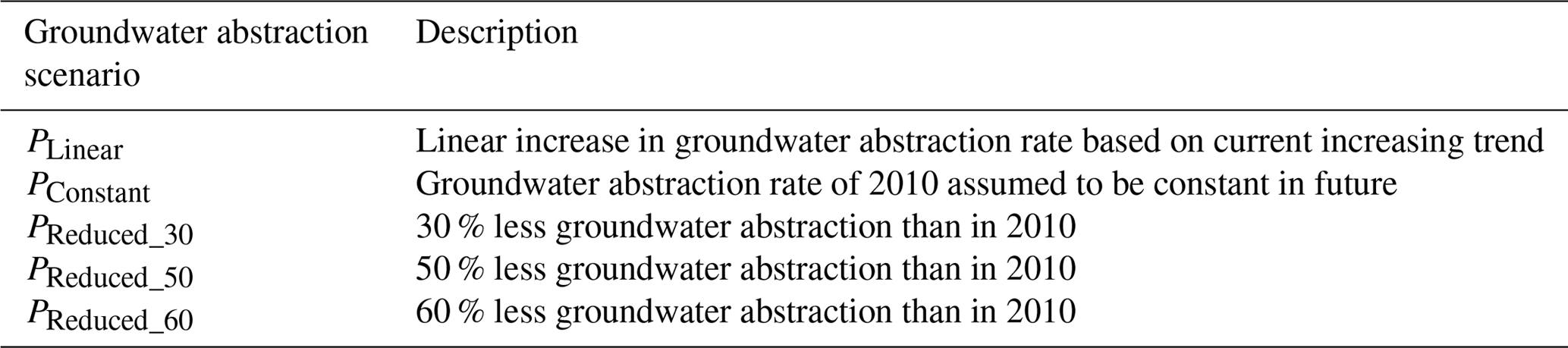
Considering the uncertainties in the total groundwater abstraction amount, five different groundwater abstraction scenarios are developed (Table 1). The first scenario is developed based on the current increasing trend. The second scenario assumes an improved irrigation water use. As such the conveyance efficiency will compensate the increasing future demand and the groundwater abstraction rate will remain constant. In other words, this scenario considers the groundwater abstraction rate for 2010. The third, fourth and fifth scenarios assume, respectively, 30 %, 50 % and 60 % lower groundwater abstraction, where the groundwater abstraction rate in 2010 was considered as a basis.

Table 1 Description of future groundwater abstraction scenarios.

2.9 Uncertainty estimation

The spread of the 95 % prediction interval was taken as the uncertainty band of the ensemble. The uncertainty band was estimated using Eq. (11).

$$\begin{array}{}\text{(11)}& {\displaystyle }& {\displaystyle }{U}_{\mathrm{band}}^n=D_{\mathrm{97.5}}^n-D_{\mathrm{2.5}}^n,\text{(12)}& {\displaystyle }& {\displaystyle }{U}_{\mathrm{avg}}={\displaystyle \frac{\mathrm{1}}{N}}\sum _{n=\mathrm{1}}^N{U}_{\mathrm{band}}^n,\end{array}$$

where $U_{\mathrm{band}}^n$ is the uncertainty band of a time step, U_avg is the average uncertainty band, N is the total number of predictions, and $D_{\mathrm{97.5}}^n$ and $D_{\mathrm{2.5}}^n$ represent the 97.5th and 2.5th percentiles of the ensemble at a time step, respectively.

In the case of alternative CHM uncertainty quantification, the same abstraction and recharge scenarios of the baseline period were used to simulate groundwater levels of the 22-year period. To quantify the recharge scenario uncertainty, the groundwater level was simulated for 44 recharge scenarios by the best-performing groundwater flow model where the groundwater abstraction scenario was kept the same. The groundwater level was simulated for five abstraction scenarios by the best-performing groundwater flow model where the same recharge scenario was used to estimate abstraction scenario uncertainty. The groundwater levels in 50 observation wells for a period of 22 years were used to estimate the spread of the 95 % prediction interval.

The contribution of the different sources of uncertainty in future groundwater-level prediction was calculated considering all the probable combinations of the CHM, recharge and abstraction scenarios. The average prediction interval at each time step was calculated using the following equations:

$$\begin{array}{}\text{(13)}& {\displaystyle }& {\displaystyle }{U}_{{\mathrm{CM}}_{\mathrm{avg}}}^n={\displaystyle \frac{\mathrm{1}}{\mathrm{AS}\times \mathrm{RS}}}\sum _{\mathrm{AS}=\mathrm{1}}^{\mathrm{AS}}\sum _{\mathrm{RS}=\mathrm{1}}^{\mathrm{RS}}{U}_{{\mathrm{CM}}_{\mathrm{AS},\mathrm{RS}}}^n,\text{(14)}& {\displaystyle }& {\displaystyle }{U}_{R_{\mathrm{avg}}}^n={\displaystyle \frac{\mathrm{1}}{K\times \mathrm{AS}}}\sum _{K=\mathrm{1}}^K\sum _{\mathrm{AS}=\mathrm{1}}^{\mathrm{AS}}{U}_{R_{K,\mathrm{AS}}}^n,\text{(15)}& {\displaystyle }& {\displaystyle }{U}_{A_{\mathrm{avg}}}^n={\displaystyle \frac{\mathrm{1}}{K\times \mathrm{RS}}}\sum _{K=\mathrm{1}}^K\sum _{\mathrm{RS}=\mathrm{1}}^{\mathrm{RS}}{U}_{A_{K,\mathrm{RS}}}^n,\end{array}$$

where $U_{{\mathrm{CM}}_{\mathrm{avg}}}^n$, $U_{R_{\mathrm{avg}}}^n$ and $U_{A_{\mathrm{avg}}}^n$ represent the average prediction interval at each time step due to CHMs, recharge scenario and abstraction scenario, respectively. The K, AS and RS represent the number of CHMs, abstraction scenarios and recharge scenarios, respectively. The $U_{{\mathrm{CM}}_{\mathrm{AS},\mathrm{RS}}}^n$ is the prediction interval due to different CHMs for a particular recharge and abstraction scenario. The $U_{R_{K,\mathrm{AS}}}^n$ and $U_{A_{K,\mathrm{RS}}}^n$ represent the prediction interval due to different recharge scenario and abstraction scenario, respectively, for a particular CHM and abstraction/recharge scenario.

2.10 Data analysis

Details about the procedure followed for data analysis are given in Sects. 2.4 to 2.9. For data analysis and plotting, different Matlab, R and Python packages were used, such as Pandas (McKinney, 2010), Scipy, ggplot2, Numpy (Walt et al., 2011) and Matplotlib (Hunter, 2007). The null hypotheses for equal distributions of simulated groundwater levels of alternative CHMs were tested using two-sample Kolmogorov–Smirnov tests (Chakravarti and Laha, 1967). The nonparametric modified Mann–Kendall trend test (Hamed and Rao, 1998) was conducted to detect trends in annual groundwater level, and the slope was estimated using Sen's method (Sen, 1968).

3 Results and discussion

3.1 Groundwater-level simulation

The simulated groundwater levels of each alternative groundwater flow model were compared to the observed groundwater levels as well as to the simulated groundwater levels of the other models. The null hypotheses for the equal distribution test between simulation results of alternative models in the calibration and validation periods were tested (Fig. 4). A significant difference (significance level of 0.05 or p<0.05) between most of the alternative model's simulation results was observed. This indicates that the use of different geological stratifications and boundary conditions in groundwater flow models can result in significant differences in groundwater-level prediction and confirms the finding of Rojas et al. (2010). In contrast, some of the models did not predict statistically different results.

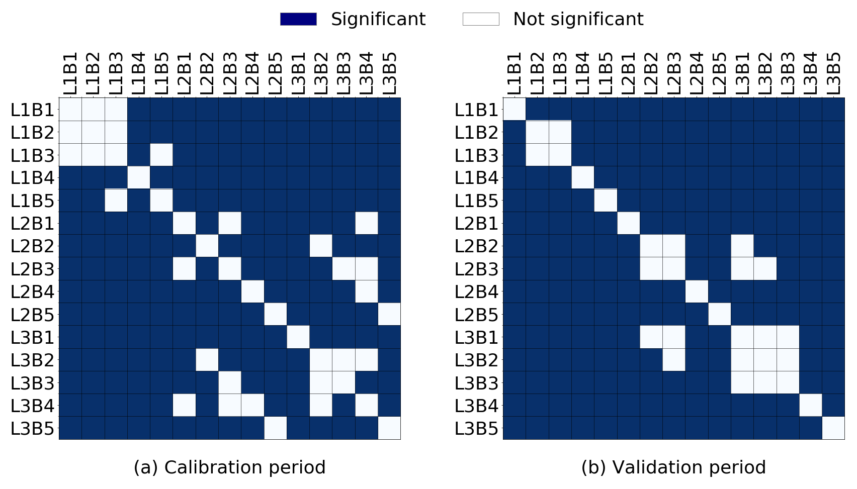
Figure 4 Significance of difference in simulation results for combinations of alternative conceptual models (p<0.05, two-sample K–S test) for (a) calibration and (b) validation periods. L1, L2 and L3 represent, respectively, the one-, two- and three-layered model. B1, B2, B3, B4 and B5 represent, respectively, Boundary condition-1, -2, -3, -4 and -5. For example: L1B1: one-layered model with Boundary condition-1; L3B5: three-layered model with Boundary condition-5.

3.1.1 Goodness of fit of alternative CHMs

Based on different statistical coefficients, the performance was different for alternative models, and the models performed differently in the calibration and validation periods (Table S5).

Based on RMSE and the NSE value, the L2B3 model was the best model in the calibration period, whereas in the validation period it was L2B5. In general, the two-layered models had a relatively lower RMSE than the one-layered and three-layered models. Overall, based on both RMSE and NSE, the two-layered models outperformed the one-layered and three-layered models in the calibration and validation periods.

The simplified one-layered models have a comparatively higher bias in prediction. Comparatively, a large number of processed parameters made the three-layered models over-parameterized. The three-layered models performed better than the one-layered models during calibration, but they performed similarly in most of the cases in the validation period. The performance of the two-layered models also differed between the calibration and validation periods. It is difficult to calibrate over-parameterized models efficiently (Willems, 2012), so the two-layered models with eight calibrated parameters can be a balance between oversimplified and over-parameterized models.

Figure 5 shows the scatter plot for model L2B5. One of the possible causes of the observed differences is the spatial and temporal variation in groundwater abstraction. The zone-wise spatially distributed groundwater abstraction rate was one of the most important input data in this study. In reality, groundwater abstraction varies spatially within those zones. Agricultural and industrial areas abstract more groundwater than wetlands or forest areas. Moreover, groundwater abstraction rate also varies in time following cropping seasons and precipitation patterns. However, an average constant groundwater abstraction rate was assumed for 6 months (from November to April) in the model. The differences between observed and simulated groundwater level are high for some observation wells. Those observation wells might be located near abstraction wells. For observation wells close to groundwater abstraction wells, drawdown by groundwater abstraction could affect observed groundwater heads. This spatial and temporal difference in actual groundwater abstraction and modelled groundwater abstraction causes spatial and temporal variation in simulated and observed groundwater levels. The simplified representation of hydrogeological layers and properties could be also a possible cause of the differences between simulated and observed groundwater levels. For simplification, the aquifer was assumed to be homogeneous, but in reality the aquifer is heterogeneous, and this may affect groundwater flow in the aquifer. Also, measurement errors in observation data may influence model performance.

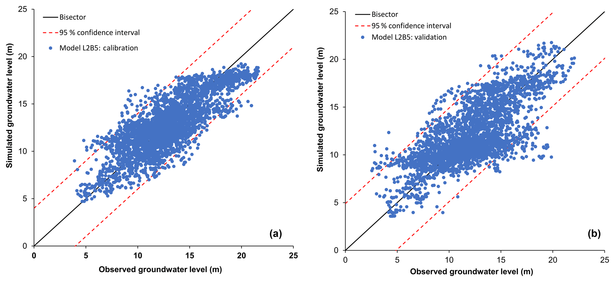
Figure 5 Scatter plot for the simulated versus observed groundwater level for Model L2B5: (a) calibration period and (b) validation period.

3.1.2 Model selection for future groundwater-level simulation and uncertainty analysis

To select the best-performing model, the simulation results of the calibration and validation periods were used to calculate information criteria statistics. The posterior probability (p_k) was calculated using Eq. (8) for the AIC, AICc, BIC and KIC methods. The L2B4 model obtained the highest posterior probability of 1, whereas all other models had a negligible posterior probability for all information criteria as shown in Fig. 6.

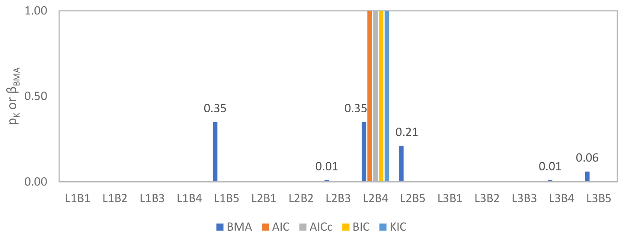
Figure 6 Posterior probability (p_k) and BMA maximum likelihood weight (β_BMA) of alternative models calculated using 10 years of data. The value above the bar represents the maximum likelihood Bayesian weight.

One of the objectives was to estimate future groundwater levels using model averaging. Ten years (1990–1999) of monthly simulated groundwater levels of the alternative models and observed data of 50 observation wells were used as training data in MODELAVG to estimate the maximum likelihood BMA weight (β_BMA) of each alternative model. The long training period was selected so that a reliable BMA weight can be estimated for climate change impact analysis.

The performance evaluation statistics of BMA mean prediction along with the best model and median are shown in the Supplement (Table S6). The best model was selected based on the information criteria ranking. The prediction of the BMA method obtained better performance in all evaluation criteria than the best model and ensemble median for both periods. The results are in line with the findings of Ye et al. (2004) and Poeter and Anderson (2005).

During the training period, the 95 % prediction interval covers about 85 % of observed data, and the average spread of the 95 % prediction interval is 6.23 m. The maximum likelihood BMA weight (β_BMA) of all alternative models is shown in Fig. 6. It is observed that models L1B5 and L2B4 obtained higher β_BMA than other models. The model L2B4 has both maximum posterior model probability and higher β_BMA. It is noteworthy that the L1B5 model obtained significant β_BMA, as it had a comparatively poor performance in both the calibration and validation periods compared to most of the other models. One possible cause could be the relatively better performance of the one-layered model in the model boundary area.

Figure 6 shows that only three models (L1B5, L2B4, L2B5) together correspond to 91 % of the total weight and another three models (L2B3, L3B4, L3B5) correspond to 8 % of the total weight. The rest of the models had no significant contribution. The models with low β_BMA can be excluded from the analysis to minimize the calculation time and effort (Vrugt, 2016). Therefore, models L1B5, L2B4 and L2B5 were selected to predict future groundwater levels under different scenarios. Ultimately, β_BMA was recalculated using the prediction of those selected models and the new β_BMA of L1B5, L2B4 and L2B5 was 0.35, 0.39 and 0.26, respectively. During this recalculation, the 95 % prediction interval covers about 82 % of observation data, meaning exclusion of 12 models resulted in a loss of only 3 % of observed data.

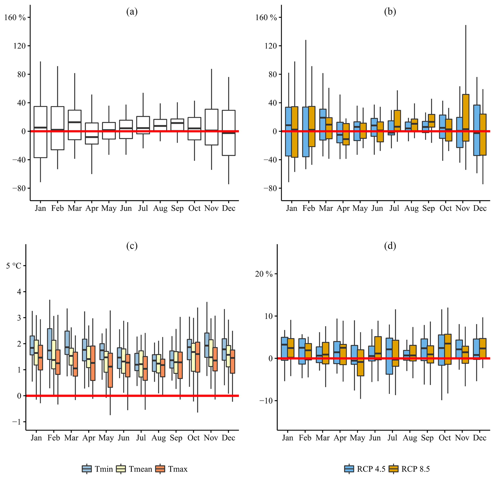
Figure 7 Climate impact signal for all selected climate models (1975–2035): (a) relative changes in monthly precipitation amount (all GHSs combined), (b) relative changes in monthly precipitation amount as a function of the GHSs, (c) absolute changes in monthly minimum, mean and maximum daily temperature (all GHSs combined), and (d) relative changes in potential evapotranspiration as a function of the GHSs.

3.2 Climate change impact on precipitation, temperature and evapotranspiration

Figure 7 shows the changes in monthly climatic parameters between the control and scenario periods ranging between 1961–1990 and 2021–2050, respectively. Figure 7a shows the changes in the monthly precipitation amount. Small positive changes in monthly precipitation amounts are observed for the wet season. For the dry season (November to April), in contrast, the changes are less consistent: decreasing precipitation amounts are found for April and December, while March displays a significant increase. The effect of the GHS on the monthly precipitation amount changes is shown by Fig. 7b. One would expect increasing/decreasing change signals under increasing GHSs. This unidirectional behaviour is, however, limited to the months July, August, September and November. Most likely, 2035 is situated before the time of emergence, whereby the effect of the increasing GHS remains mainly masked by noise inherent to the internal climate variability (Hawkins and Sutton, 2012). This, moreover, indicates that the months July, August, September and November are most likely more sensitive to the GHSs compared to the other months.

Figure 7c presents the climate scenarios for minimum, mean and maximum daily temperature. It shows the absolute changes in monthly minimum, mean and maximum daily temperature between the control and scenario periods. Generally, higher increases in minimum and mean daily temperatures are projected during the wet season. An inter-comparison between the different variables shows, furthermore, higher changes for the minimum daily temperature than for the mean and maximum daily temperature.

The changes in monthly potential evapotranspiration are shown in Fig. 7d. Except for May, increases are observed for all months. For some months, the changes seem not sensitive to the GHS. Changes for the months March, April, June, October and December seem particularly sensitive to the GHS. Similarly to the precipitation results, a possible explanation can be found in the “time of emergence” concept.

The climate change signals for a representative month in the dry and wet seasons are included in Table S8.

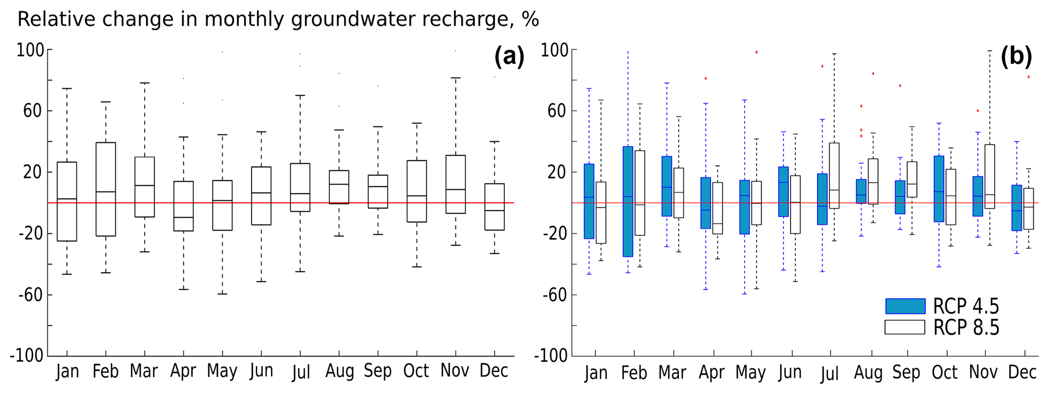
Figure 8 Change in groundwater recharge due to climate change: (a) relative changes in monthly groundwater recharge (all GHSs combined); (b) relative changes in monthly groundwater recharge as a function of the GHSs.

3.3 Climate change impact on groundwater recharge

The changes in the monthly groundwater recharge due to climate change are highly uncertain (Fig. 8a). Like precipitation, small increasing changes in monthly groundwater recharge are observed for the wet season. For the dry season (November to April), in contrast, the changes are less consistent. The majority of the global climate model runs project generally an increasing groundwater recharge. However, for April and December, significant decreases are noted. The effect of the GHSs on the monthly groundwater recharge changes is shown by Fig. 8b. The months July, August, September and November seem to be more sensitive to the GHSs compared to the other months. For both RCP 8.5 and RCP 4.5, April and December show decreasing changes in monthly groundwater recharge.

Projected spatial variation of the mean groundwater recharge change between the future and baseline periods due to climate change is presented in Fig. 9. Spatial variation is observed only for two extreme recharge scenarios: high recharge scenario indicates maximum recharge at each time step among all the ensembles and low recharge scenario indicates minimum recharge. For both April and September, the high recharge scenario shows a zero to positive change in groundwater recharge, while the low recharge scenario shows a zero to negative change in groundwater recharge. No clear spatial trends are observed in the change in groundwater recharge. In the high recharge scenario, mean monthly groundwater recharge would increase by 25 mm (April) and 100 mm (September). In the low recharge scenario, mean monthly groundwater recharge would decrease by 16 mm (April) and 35 mm (September). Crosbie et al. (2010), also, reported that changes in groundwater recharge due to climate change are uncertain.

Figure 9 Spatial variation of mean groundwater recharge change due to climate change for (a) a high recharge scenario in April, (b) a low recharge scenario in April, (c) a high recharge scenario in September and (d) a low recharge scenario in September.

3.4 Future groundwater-level analysis

The baseline and future groundwater levels were simulated using three selected groundwater flow models (L1B5, L2B4, L2B5). Then, the model average was calculated by Eq. (1) using simulated groundwater levels and the maximum likelihood Bayesian weight of the respective groundwater flow models. The change in groundwater level for different scenarios is discussed below.

3.4.1 Baseline groundwater-level simulation

Groundwater levels in the baseline scenario show a decreasing trend. The mean decreasing rate of groundwater level is 0.18 m/year (Sen's slope). The summary of the trend analysis for 50 observation wells is shown in the Supplement (Table S9). The calculated decreasing rate varies spatially and ranges between 0.05 and 0.49 m/year. Mustafa et al. (2017b) studied observed groundwater-level data of the same study area and reported that the average groundwater level dropped by 4.5–4.9 m over the last 29 years at a rate of 0.15–0.17 m/year. The annual groundwater-level fluctuation of 3 to 5 m in the baseline scenario is also supported by the findings of Shamsudduha et al. (2009). Overall, the simulated groundwater levels correspond well to the findings of other researchers for the baseline period. Therefore, the simulated groundwater level of the baseline period was used for comparison with the simulated groundwater levels of the future scenarios.

3.4.2 Impact of climate change on groundwater level

The impact of climate change on groundwater level is highly uncertain in the study area (Fig. 10a). The uncertainty ranges of the change in mean monthly groundwater level due to different GCMs and GHSs obtained from the three selected conceptual groundwater flow models are presented with the box-plot for each month. Climate change could increase the mean monthly groundwater level by up to 2.5 m and could decrease it by 0.5 m. However, the SDGs suggest a 0–0.5 m increase in groundwater level due to climate change. The impact of climate change seems higher from May to September than from October to April. This seasonal variation of climate change impact can be explained by the precipitation pattern of the study area (Fig. S2a). Large precipitation amounts occur from May to October in Bangladesh, so that climate change has a higher impact in this period. Uncertainty of groundwater level due to climate change is highest from June to December. The precipitation pattern can also explain the monthly variation of climate change impact uncertainty. Groundwater levels increase more during the rainy season in a high recharge scenario (high precipitation), but in a low recharge scenario, groundwater levels decrease due to the lack of recharge in the rainy seasons. Therefore, the uncertainty band increases in this period for extreme scenarios. Similarly to precipitation and groundwater recharge, the effects of the GHSs are not very significant on groundwater-level changes (Fig. 10b). Most of the GCMs project that the increase in groundwater level would be higher for RCP 8.5 compared to RCP 4.5 for all months.

Figure 10 Mean monthly change in groundwater levels in the simulated future period (2026–2047) compared to the baseline period (1980–2006) due to climate change: (a) all GHSs combined, and (b) as a function of the GHSs.

The impact of climate change on groundwater level also varies spatially. The projected impact of climate change on groundwater level is relatively higher in the southwestern part (Fig. 11), although this pattern does not correspond to the spatial pattern of groundwater recharge (Fig. 9). This can be explained by the effect of the river on groundwater level. In a high recharge scenario mean monthly groundwater level would increase up to 4 m (April) and 8 m (September). However, in a low recharge scenario, mean monthly groundwater level would decrease down to 1.6 m. Overall, the impact of climate change on groundwater level was not linear.

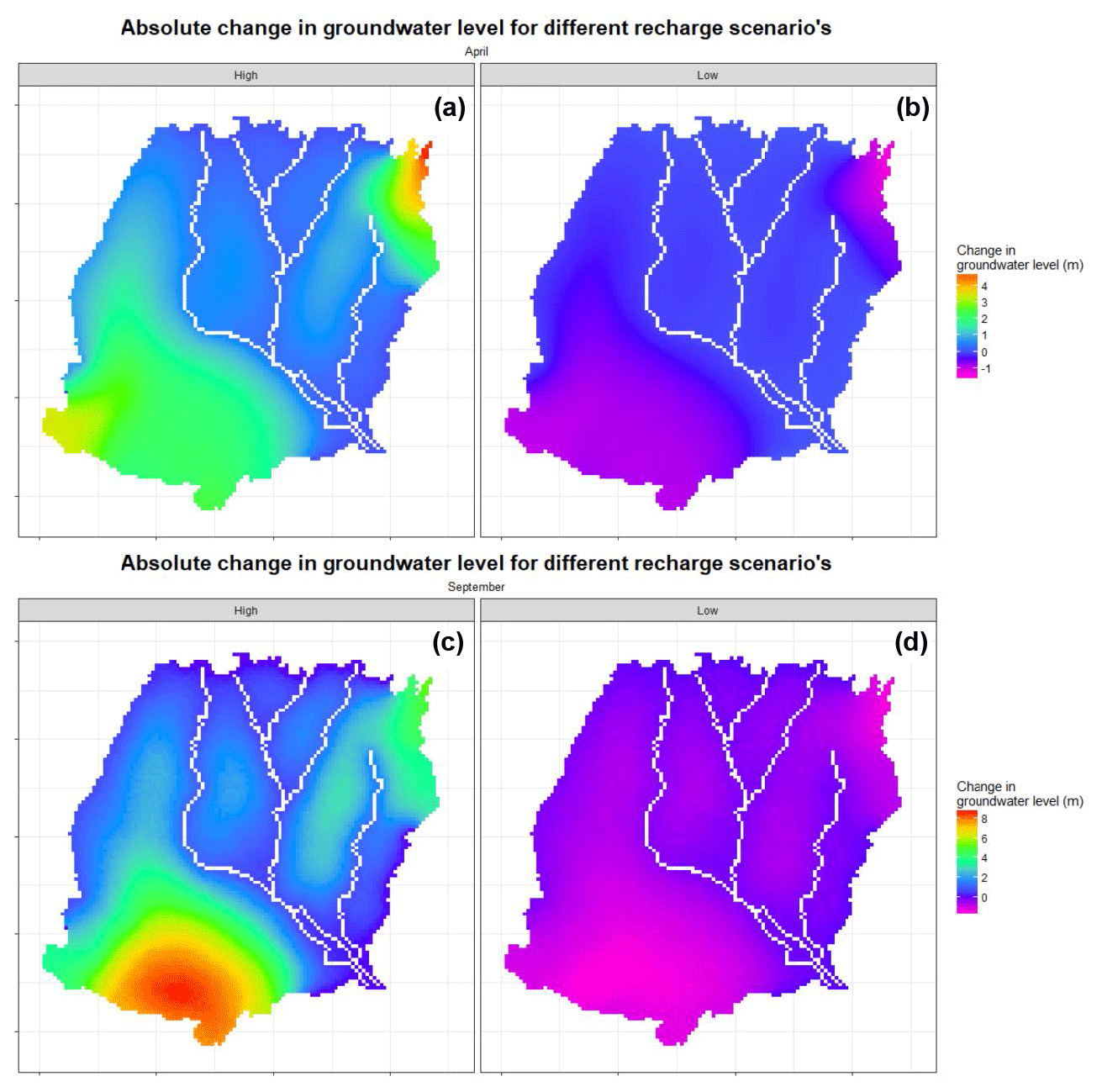
Figure 11 Spatial variation of mean groundwater-level change due to climate change for the (a) high recharge scenario in April, (b) low recharge scenario in April, (c) high recharge scenario in September, and (d) low recharge scenario in September.

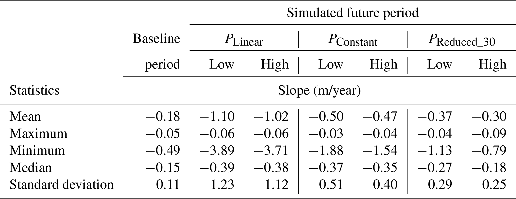
Table 2 The summary of annual groundwater-level trend statistics of 50 observation wells for the baseline (1985–2006) and simulated future (2026–2047) periods under different abstraction scenarios (P_Linear, P_Constant, P_{Reduced_30}) and recharge scenarios (low, high).

3.4.3 Future groundwater levels under different abstraction scenarios

The mean monthly groundwater level for the P_Linear abstraction scenario decreases about 10 to 14 m compared to the baseline period (Fig. 12a). The scenario of P_Constant resulted in a 4 to 7 m decrease in groundwater level (Fig. 12b). For the 30 % reduced (P_{Reduced_30}) abstraction scenario, the mean groundwater level would decrease about 1.5 to 3.8 m (Fig. 12c). Even for the 50 % reduced (P_{Reduced_50}) abstraction scenario, the mean groundwater level would decrease about 1.0 to 1.5 m (Fig. 12d). Groundwater abstraction in the study area has to be reduced by 60 % compared to the groundwater abstraction rate in 2010, to keep a sustainable groundwater level (Fig. 12e). This indicates that the groundwater abstraction rate of 2010 is much higher than the future recharge potential. The situation will be worse if the current increasing groundwater abstraction trend continues. A spatial variation in groundwater-level change for different abstraction scenarios was also observed. In a low recharge scenario, even for a 30 % reduced (P_{Reduced_30}) abstraction scenario, groundwater level decreased about 14 m in the southwestern part of the study area. In a high recharge scenario, on the other hand, groundwater level increased about 2 m in the northeastern part of the study area for the P_{Reduced_30} abstraction scenario. The results also show that a 50 % lower groundwater abstraction than the 2010 rate is not enough to stop groundwater level declining in the southwestern part of the study area.

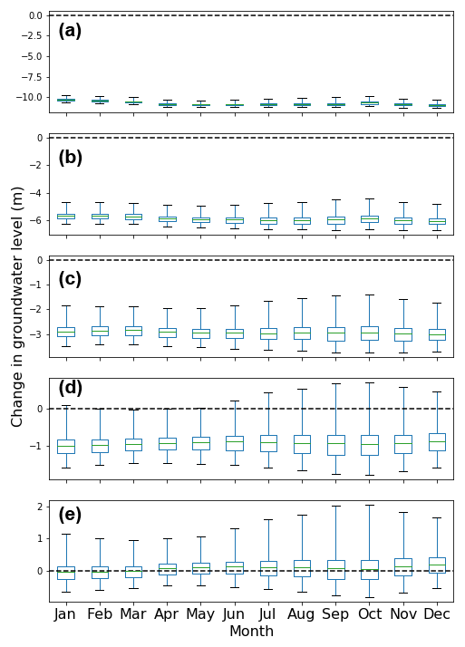
Figure 12 Monthly mean change in groundwater levels in the simulated future period (2026–2047) compared to the baseline period (1985–2006) due to groundwater abstraction: (a) for the P_Linear abstraction scenario; (b) for the P_Constant abstraction scenario; (c) for the 30 % reduced (P_{Reduced_30}) abstraction scenario; (d) for the 50 % reduced (P_{Reduced_50}) abstraction scenario; and (e) for the 60 % reduced (P_{Reduced_60}) abstraction scenario.

The summary of annual groundwater-level trend analysis of 50 observation wells for the high- and low-recharge scenarios and for different abstraction scenarios (P_Linear, P_Constant, and P_{Reduced_30}) is shown in Table 2. Only the significant (p<0.05) trends were considered in this analysis. Scenarios P_Constant and P_{Reduced_30} have a mean decreasing rate that is 2 to 3 times higher than the baseline scenario. Therefore, proper groundwater abstraction policy is necessary to maintain sustainable use of this resource.

3.5 Sources of uncertainty in groundwater-level prediction

3.5.1 Alternative conceptual model (CHM) uncertainty

The 95 % prediction intervals of the three best-performing models are shown in Fig. 13a. The average spread of the 95 % prediction interval of the three alternative CHMs was about 3 m with a maximum spread of about 16 m. It is observed that the spread of the prediction interval is wider for low and high groundwater levels. This is not surprising as the one-layered model overestimates low groundwater levels and underestimates high groundwater levels in most of the observation wells. The wide uncertainty band of the alternative CHMs indicates that the use of a single model in groundwater-level prediction may lead to biased conclusions.

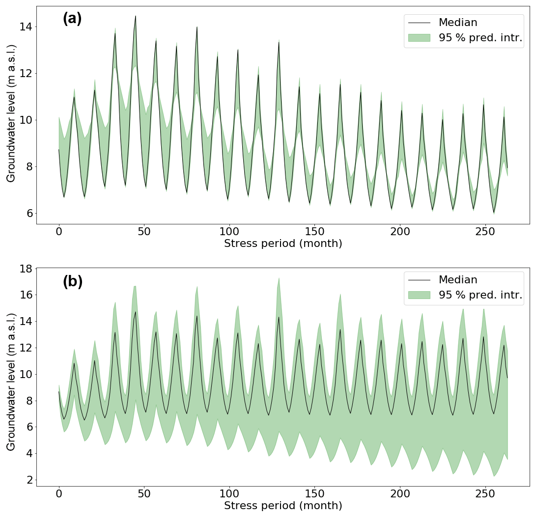
Figure 13 The 95 % prediction interval of groundwater level of a representative observation well (BOG001) for (a) different conceptual models and (b) different abstraction scenarios.

3.5.2 Recharge scenario uncertainty

The average spread of the 95 % prediction interval due to recharge scenarios is 1.11 m with a maximum of 6.07 m. The predictive uncertainty due to the recharge scenario is higher during periods with high groundwater levels and recharge. Although the mean uncertainty resulting from recharge scenarios is relatively lower than for other sources of uncertainty, there is large temporal and spatial variation in groundwater-level prediction due to recharge scenarios (as described in Sect. 3.4.2). The recharge scenarios were developed using future climate scenarios of different climate models so that the uncertainty from recharge scenarios represents the uncertainty from climate scenarios in groundwater-level prediction. This uncertainty analysis suggests that all possible climate scenarios should be considered to predict groundwater levels with a reliable uncertainty band.

3.5.3 Abstraction scenarios uncertainty

The 95 % prediction interval of groundwater level for different abstraction scenarios increases with time (Fig. 13b). The average spread of the 95 % prediction interval is 8.38 m and the maximum is 43 m. The uncertainty of groundwater level related to the abstraction scenario is very high.

3.5.4 Comparison of sources of uncertainties

The uncertainties due to alternative CHMs, recharge scenarios and abstraction scenarios are compared (Fig. 14). The spread of the prediction interval of groundwater levels resulting from different CHMs, recharge scenarios and abstraction scenarios was estimated using Eqs. (13), (14) and (15), respectively. The contribution of each source was calculated based on the median value of the spread of the prediction interval. The contribution of an individual source is calculated as the ratio of the median value of the spread of the prediction interval for the respective source to the median value of the spread of the prediction interval for the total uncertainty. The abstraction scenarios are the dominant source of the total uncertainty in groundwater-level prediction in this overexploited aquifer. About 68 % of the total uncertainty arises from the abstraction scenarios. CHM uncertainty contributed about 23 % of total uncertainty. This result is in agreement with the findings by Rojas et al. (2008). They reported CHM uncertainty contributions up to 30 %. In this case, the alternative CHM uncertainty contribution is higher than the recharge scenario uncertainty contribution, including the greenhouse gas scenario, climate model and stochastic climate uncertainty contributions. Goderniaux et al. (2015) reported that uncertainty related to the calibration of hydrological models can be more important than uncertainty related to climate models in groundwater modelling. The uncertainty due to recharge scenarios was relatively lower than the other sources, but the uncertainty arising from recharge scenarios was very high in the southwestern part of the study area (described in Sect. 3.4.2). Hence, use of a single model or single recharge or abstraction scenario may lead to biased estimation of groundwater levels. Therefore, a multi-model and multi-scenario approach should be used for reliable groundwater-level prediction.

Figure 14 Comparison of uncertainties arising from alternative conceptual models, recharge scenarios and abstraction scenarios. The recharge scenario uncertainty includes the greenhouse gas scenario uncertainty, the climate model uncertainty and the stochastic uncertainty.

4 Conclusions

The main objective of this study was to quantify groundwater-level prediction uncertainty in climate change impact studies using an ensemble of representative concentration pathways, global climate models, multiple alternative CHMs and abstraction. In this study, 15 alternative CHMs, 22 climate model runs for representative concentration pathways 4.5 and 8.5 (in total 44 climate model runs) and 5 groundwater abstraction scenarios were used to achieve this aim. The BMA technique was used to predict reliable groundwater level using predictions of alternative CHMs.

It was observed that different conceptual groundwater models (CHMs) can simulate significantly different groundwater levels due to differences in the number of layers and the boundary conditions. The simple one-layered models were unable to simulate seasonal variation, but had a relatively better performance close to the model boundaries than the other multi-layered models. The three-layered models were more detailed, but the performance was not superior to the two-layered models. The performance of the two-layered models was mostly better than the one-layered and three-layered models.

Ranking of models differed in the calibration and validation period. The best model in the calibration period only got the 4th rank in the validation period, suggesting the importance of the use of multiple CHMs for reliable prediction.

The impact of groundwater abstraction on groundwater levels is very high. For 2026–2047, the groundwater level would decline about 5 to 6 times faster than in the baseline period (1985–2006) if the current increasing groundwater abstraction trend continues. Even with a 30 % lower groundwater abstraction rate compared to the 2010-rate, the mean monthly groundwater level would decrease by up to 14 m in the southwestern part of the study area. Groundwater abstraction has to be reduced by 60 % compared to the 2010-rate to keep groundwater level sustainable. This indicates that the groundwater abstraction rate of 2010 was far higher than recharge potential.

The differences in groundwater abstraction scenarios were the dominant source of uncertainty in groundwater-level prediction. The uncertainty due to alternative CHMs was also found to be significant and higher than the uncertainty from the recharge scenarios. The uncertainty due to different recharge scenarios was very high in the southwestern part of the study area. Therefore, use of a single model and/or single recharge and abstraction scenario can lead to biased groundwater-level prediction.

This study suggests that a multi-model approach should be used in groundwater-level prediction to avoid biased estimation of groundwater levels. The BMA is probably the most suitable technique for developing a multi-model average based on the best available data and future alternative scenarios. This study recommends that the uncertainty due to alternative CHMs, recharge and abstraction scenarios should be considered in future groundwater-level prediction.

In this study, alternative conceptual models have been calibrated using PEST. However, different calibration methods can result in different calibrated model parameters. Hence, further studies could be conducted using different calibration methods (e.g. global parameters' optimization methods). We also suggest that more field data be collected, such as reliable groundwater abstraction data, river flow information, spatially distributed horizontal hydraulic conductivity and detailed information about the boundary conditions.

Keeping in mind that the complexity of hydrogeological models is increasing, further studies should be conducted on global sensitivity analysis (SA) to (i) identify the influential and non-influential parameters on the model prediction and (ii) better understand the importance of the different components of the complex model structure. Identification of influential parameters will play an important role in model parameterization and in reducing uncertainty due to over-parameterization. The identification of non-influential parameters using SA will be a very important step in simplifying model structure.