Technical note: Changes in cross- and auto-dependence structures in climate projections of daily precipitation and their sensitivity to outliers

Simulations of regional or global climate models are often used for climate change impact assessment. To eliminate systematic errors, which are inherent to all climate model simulations, a number of post-processing (statistical downscaling) methods have been proposed recently. In addition to basic statistical properties of simulated variables, some of these methods also consider a dependence structure between or within variables. In the present paper we assess the changes in cross- and auto-correlation structures of daily precipitation in six regional climate model simulations. In addition the effect of outliers is explored making a distinction between ordinary outliers (i.e. values exceptionally small or large) and dependence outliers (values deviating from dependence structures). It is demonstrated that correlation estimates can be strongly influenced by a few outliers even in large datasets. In turn, any statistical downscaling method relying on sample correlation can therefore provide misleading results. An exploratory procedure is proposed to detect the dependence outliers in multivariate data and to quantify their impact on correlation structures.

1 Introduction

The investigation of climate change impact on the hydrological cycle is one of the crucial topics in the field of water resources management and planning (Mehrotra and Sharma, 2015). Simulations of regional and global climate models (RCMs and GCMs) represent a fundamental data source for climate change impact studies. It is well known that raw climate model outputs cannot be used directly in impact studies due to inherent biases which are found even for basic statistical properties (Chen et al., 2015). The bias is caused primarily by a simplified representation of important physical processes (Solomon et al., 2007), which often results from low spatial resolution of the RCMs.

Therefore, many methods have been developed to post-process the climate model outputs in order to move their statistical indicators closer to observations. An overview of these methods is presented, e.g. by Maraun et al. (2010). Precipitation is a key input into hydrological climate change impact studies and at the same time it belongs to meteorological variables that are most affected by bias. The comparison of correction methods commonly used for precipitation data is provided by Teutschbein and Seibert (2012). Nevertheless, these standard methods correct only the bias in statistical indicators (mean, variance, distribution function) of individual variables. The bias in persistence parameters of time series as well as the bias in cross-dependence structures between variables is often neglected. However, the dependence structures of the meteorological variables affect the hydrological response of a catchment (Bárdossy and Pegram, 2012), and thus their inadequate representation in the data can impair hydrological impact studies (Teng et al., 2015; Hanel et al., 2017).

In recent years several studies attempted to overcome this limitation. Hoffmann and Rath (2012) and Piani and Haerter (2012) focused on the relationship between precipitation and temperature data from a single location. Bárdossy and Pegram (2012) developed two procedures correcting a spatial correlation structure of RCM precipitation. Mao et al. (2015) proposed a stochastic multivariate procedure based on copulas. Johnson and Sharma (2012) developed a procedure correcting common statistics (mean, variance) together with lag-1 autocorrelation in multiple timescales. The procedure was later extended with a recursive approach by Mehrotra and Sharma (2015) and subsequently with a non-parametric quantile mapping by Mehrotra and Sharma (2016) to correct the bias in auto- and cross-dependence structures across multiple timescales. An approach based on the principal components was presented by Hnilica et al. (2017), correcting bias in cross-covariance and cross-correlation structures.

This study is focused on a temporal stability of dependence structures. We evaluate the temporal changes in cross-and auto-correlation structures in multivariate precipitation data simulated by an ensemble of climate models. We further investigate whether the magnitude of the changes considerably exceeds the natural variability. Attention is finally paid to the effect of outlying values, which can significantly affect the correlations and can thus lead to artefacts in bias-corrected time series.

The paper is organised as follows. In Sect. 2 the data used in this study are presented and Sect. 3 describes the methodology. In Sect. 4 the results are reported and in Sect. 5 their consequences for climate changes impact studies are discussed.

2 Data and study area

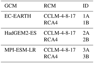
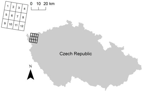
The daily precipitation data from six EURO-CORDEX (Giorgi et al., 2009) regional climate models were considered. The ensemble of models was composed of two RCMs (CCLM,RCA) driven by three GCMs (EC_EARTH, HadGEM2-ES and MPI-ESM-LR); see Table 1 for the overview. The simulations with 0.11 ^∘ spatial resolution forced by the representative concentration pathway 8.5 (RCP8.5) were used. The data from 12 model grid boxes located in the western part of the Czech Republic were analysed; see Fig. 1 for the details of the area. The control period spans the years from 1971 to 2000, the future period the years from 2051 to 2080.

Table 1 Global and regional climate models used in the present study.

Figure 1 Location of the considered grid boxes in the Czech Republic.

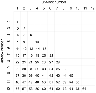
Figure 2 The numbering of individual pairs of grid boxes. The figure depicts the correlation matrix, the orders of rows and columns correspond to the grid box labels from Fig. 1. The sub-diagonal part of the (symmetrical) matrix was used for the numbering of individual pairs of grid boxes – the numbers inside of the matrix represent the identifiers used in Fig. 4.

Figure 3 Overview of the changes in correlation structures for all models: (a) the changes in binary cross-correlations, (b) the changes in cross-correlations of overlapping wet periods, (c) the changes in lag-1 auto-correlations.

3 Methods

The wet and dry periods were treated separately in this study. The cross-correlations were calculated in two stages. Firstly the binary cross-correlations were calculated to assess the correspondence of wet and dry periods, using the time series with the values replaced by 0 (dry day) or by 1 (wet day). In the second stage the cross-correlations of overlapping wet periods were calculated. The auto correlations were analysed through the lag-1 auto-correlation coefficient, where only the non-zero pairs of neighbouring values x_i and x_i+1 were considered.

The individual grid boxes were labelled by numbers 1–12, as shown by labels in Fig. 1. The cross-correlation between the grid boxes i and j is denoted as r_i, j. The symbol R denotes the correlation matrix (i.e. the square matrix with elements r_i, j). The lag-1 auto-correlation from grid box i is denoted as $r_i^{\mathrm{1}}$. If appropriate, the subscripts denoting the grid boxes are omitted for clarity.

The changes in correlation coefficients were calculated as

$$\begin{array}{}\text{(1)}& \mathrm{\Delta }r=r_{\mathrm{F}}-r_{\mathrm{C}},\end{array}$$

where Δr denotes the change in r (cross- or auto-correlation), and subscripts F and C denote the future and control periods, respectively. Note that the first-order moments needed for calculation of r_F and r_C are calculated independently for the future and control periods. Another option, leading potentially to larger changes, is to consider a fixed reference, e.g. the mean for the control period. However, the changes in the mean are relatively small; the average change is 0.14 mm across all considered simulations, which represents approximately 5 % of the value from the control period. Therefore the differences in the calculated Δr and their significance are not expected to be large.

The sampling variability of individual cross- and auto-correlation was investigated to assess the statistical significance of their changes. The confidence intervals were derived using the block bootstrap approach (Davison and Hinkley, 1997). Specifically, the confidence interval around the correlation r_i, j was obtained as follows:

1. One-year blocks from the time series for basins i and j were randomly selected with replacement (30 times to obtain the same sample size as the original data). Subsequently the correlation of the 30 year sample was calculated.

2. Step 1 was repeated 1000 times.

3. The 95 % confidence interval was derived as a range between the 0.025 and 0.975 quantiles of the resampled correlations.

The block approach was chosen to preserve seasonal variability in the bootstrap samples. For the presentation of confidence intervals, the unique identifier (ID) was assigned to each pair of grid boxes, and the numbering was done according to rows of correlation matrix; the scheme is depicted in Fig. 2. The confidence intervals for auto-correlation were derived in the same way using 1-year blocks of time series. Due to random selection of the blocks, the beginning part of the blocks is independent on the end of the previous block. To minimise bias introduced by block resampling, data that are potentially influenced (joints of the adjacent blocks) were not considered for the calculation of the serial correlation.

The confidence intervals around the correlations from control and future period were used to visually assess their overlap. In addition, the real bootstrap-based tests of significance of individual changes were performed. In each of the thousand steps the correlation of resampled control data was subtracted from the correlation of resampled future data. The change was found to be insignificant if the confidence interval of these differences contained zero.

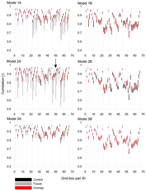
Figure 4 The 95 % confidence intervals of the individual cross-correlation coefficients for overlapping wet periods for all models. The identifiers of grid-box pairs (ID) are explained in Fig. 2. The blue lines separate identifiers located in successive rows in the correlation matrix (see Fig. 2). The arrow marks the confidence intervals around the r_5, 11 (ID 50) of the model 2A, discussed in more detail in Sect. 4.2.

4 Results

4.1 Changes in correlation structures

In the case of 12-dimensional data, the change in the cross-correlation structure consists of changes in r_i, j coefficients for 66 pairs of grid boxes (corresponding to the sub-diagonal part of the correlation matrix). For clarity, these 66 changes are presented in the form of box plots for individual models.

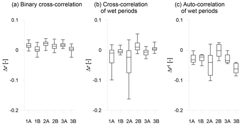
Figure 3a and b present the changes in the binary cross-correlations and in the cross-correlations of wet periods, respectively. As seen from the figures, the binary correlations are relatively stable; their changes range approximately from −0.02 to 0.03. Therefore, the correspondence of wet and dry periods between individual grid boxes remains similar in the control and future periods. The correlations of wet periods change more substantially; the changes range from −0.16 to 0.05. Nevertheless, there are strong differences between individual models; the models 1A and 2A reach noticeably higher changes than other models. In addition, the changes in fractions of dry days were calculated. In general, the fraction of zeroes fluctuates around 0.25 in time series across all models and it was found that it slightly increases in most cases. The difference can be found between the regional models A and B. While in the simulations of the model A the fractions of zeroes increase on average by 0.05; for the model B the average increment is only 0.009.

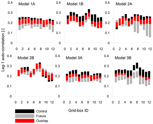
Figure 5 The 95 % confidence intervals of the individual lag-1 auto-correlation coefficients for all models.

Figure 3c presents the changes in lag-1 auto-correlations; the box plots for individual models are compiled from 12 changes in time series from individual grid boxes. The changes range from −0.1 to 0.025; the widest range of changes is reached by the model 2A. The maximal relative changes in cross-correlation reach up to 18 % of the value from the control period, and in the case of auto-correlation it is almost 45 %. This is because the auto-correlations are in general markedly lower than cross-correlations (the mean cross-correlation of individual models exceeds 0.8; the mean lag-1 auto-correlation is around 0.23). In addition, it is worth noting that the reported changes do not completely characterise the changes in the auto-dependence structure. Substantial changes in dependence at longer temporal scales have been reported in several studies (Mehrotra and Sharma, 2015, 2016; Hanel et al., 2017).

The significance of the changes in wet-period correlations was assessed using a block bootstrap. Figure 4 presents the 95 % confidence intervals of individual cross-correlations for all models. The blue dividers identify the successive rows below the diagonal in the correlation matrix. In general, the majority of changes show little significance; the intervals from control and future periods overlap considerably (except models 1A and 2A, which in many cases show exceptionally wide intervals for the future period). Figure 5 shows the same for lag-1 auto-correlations of individual grid boxes. Also in this case the majority of changes do not exceed the sampling variability; the most significant changes are reached by the model 3B, but the overall trend is a drop in the future.

To verify these results, the significance of individual changes was tested using the bootstrap approach. The results of tests correspond well with the visual assessment presented in Figs. 4 and 5. In the case of cross-correlations, only four changes were found significant for the model 1A, no changes for the model 1B, two for the model 2A, eight for the model 2B, two for the model 3A and no changes for the model 3B. In case of auto-correlations, the significant changes were found only for the model 3B. Note, however, that the fraction of significant changes might be larger in the case of a fixed reference being used for calculating correlations and auto-correlations (see Sect. 3).

4.2 Effect of outliers

The previous section demonstrated that in some cases the changes in cross-correlation show little significance despite their high absolute values, which is particularly related to the models 1A and 2A. At the same time, it can be seen in Fig. 4 that some confidence intervals for these models are exceptionally wide. Further analyses showed that this instability of correlation estimates is introduced by outlying values, which cause seeming changes in the correlation structures.

In the simulation of the model 2A, the sample correlation r_5, 11 decreased from 0.90 in the control period to 0.73 in the future period. Figure 6a depicts the data from the future period (values from the grid box 5 plotted against values from the grid box 11; the data with any zero values are excluded). The decrease is in large part caused by one outlying point, which is circled in the plot. Its removal from the data increases the correlation in the future period to 0.86, which markedly reduces the change. On the other hand, high values do not necessarily affect the correlation, as seen in Fig. 6b, where the data from grid boxes 11 and 12 are plotted (again the model 2A, future period). The circled outlier does not affect the correlation in this case, since the location of the point is in accordance with the configuration of the data – the point lies approximately in a direction of a potential regression line.

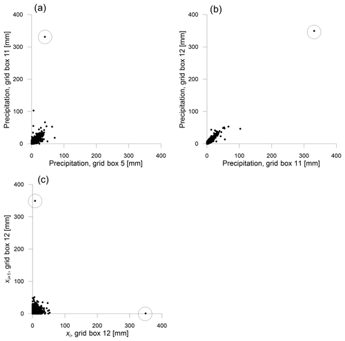
Figure 6 The effect of outliers on correlation structures of model 2A in the future period (the outliers are circled): (a) the outlier strongly affecting the cross-correlation, (b) the outlier with no effect on the correlation, (c) the outlier affecting the calculation of the serial correlation $r_{\mathrm{12}}^{\mathrm{1}}$.

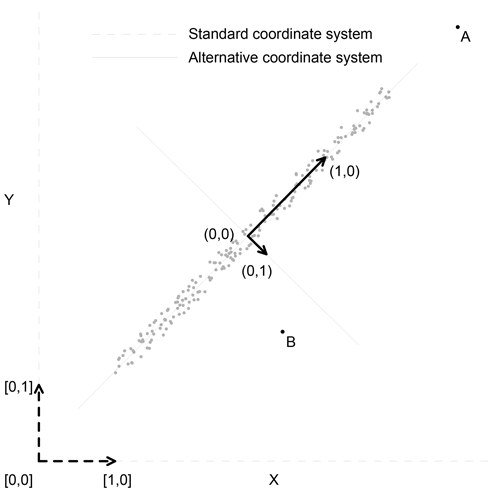
Figure 7 The difference between the ordinary and dependence outliers. The dashed lines define the standard coordinate system; the solid lines define an alternative coordinate system. The outlying points in the standard coordinate system are ordinary outliers (point A); the outlying points in the alternative coordinate system are denoted as dependence outliers (point deviating from the dependence structure, point B). The construction of alternative coordinates is explained in the text.

Outlying values affect also the auto-correlation. The largest change in the auto-correlation was achieved by the model 2A, where $r_{\mathrm{12}}^{\mathrm{1}}$ decreased from 0.23 in the control period to 0.12 in the future period. This decrease is caused by the outlier 349.4 mm in the future data; this extraordinary value was simulated by the model 2A for 8 May 2080. Figure 6c depicts the data for the calculation of $r_{\mathrm{12}}^{\mathrm{1}}$, i.e. the values x_i plotted against the values x_i+1, where i denotes the order of the value x in the time series. The outlier is employed twice within the calculation (as x_i and as x_i+1, circled values in Fig. 6c), which markedly affects the result. If the outlier is removed from the time series, $r_{\mathrm{12}}^{\mathrm{1}}$ increases from 0.12 to 0.22, which reduces the change almost to zero. The calculation of other members of the auto-correlation function is affected by the outlier in the same way. We note that the effect of an outlier on the auto-correlation strongly depends on the values which the outlier is surrounded by in the time series. The presence of a noticeable outlier thus makes the calculation of the auto-correlation very unstable.

4.3 Detection of outliers

The examples showed that outliers can distort cross- and auto-correlation structures of a large dataset comprising many thousands of values. Nevertheless, it should be realised that not each extreme value necessarily affects the correlation (as seen in Fig. 6b). Therefore, a more specific concept of outliers is presented in this study. Values deviating from the correlation structure are denoted as dependence outliers. As well as ordinary outliers, the dependence outliers are values which are a long distance from the origin; nevertheless, the difference between them and ordinary outliers depends on the coordinate system in which the distance is measured. Figure 7 illustrates this by an example of synthetic two-dimensional data. The dashed lines and coordinates in square brackets define the standard (canonical) coordinate system. The ordinary outliers are points a long distance from the origin [0, 0], measured in standard coordinates; the point A represents an example. The solid lines and coordinates in round brackets define an alternative coordinate system, which reflects the intensity of linear dependence between the variables X and Y. The dependence outliers are points a long distance from the origin (0, 0), measured in alternative coordinates; the point B represents an example. Let us remark that the point B is an extreme value neither in X nor Y data, which is in contrast to the point A. Nevertheless, the point B deviates from the dependence structure, which becomes apparent when its distance from (0, 0) in alternative coordinates is calculated. The alternative coordinate system is constructed through the covariance matrix of the data. The directions of the axes are given by the eigenvectors of the matrix, the lengths of unit vectors are given by the square root of the corresponding eigenvalues and the origin is located in the mean of the data. The construction of the system is related to the principal component analysis; see for example Wilks (2011) for details.

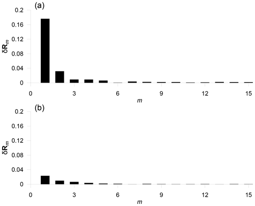
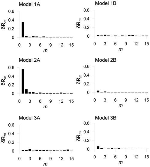
Figure 8 The demonstration of the exploratory procedure: (a) the detection of dependence outliers for two-dimensional data from Fig. 6a (the plot of δR_m indicates a noticeable outlier in the data). (b) the same for the data from Fig. 6b – a gradual evolution of δR_m indicates that data do not contain dependence outliers.

The problem is that the presence of outliers is not easily detected from the changes in dependence structures. It can be indicated indirectly from the analysis of sampling variability; nevertheless, the wide confidence intervals do not necessarily imply the presence of outliers. Or alternatively, it can be found when the individual pairs of datasets are visually checked. We propose a procedure allowing for identification of significant dependence outliers and assessment of their effect on correlation structure. The procedure consists of three steps:

1. The most outlying (multivariate) value is found in the data (in alternative coordinates).

2. The value is removed from the data and a new correlation matrix is calculated.

3. A difference between the new and the previous correlation matrix is calculated and recorded.

These three steps are repeated. The difference in step 3 is quantified through

$$\begin{array}{}\text{(2)}& \mathit{\delta }{\mathbf{R}}_m=∥{\mathbf{R}}_m-{\mathbf{R}}_{m-\mathrm{1}}∥,\end{array}$$

where R_m denotes the correlation matrix of the data from which m largest outliers were removed; the notation ∥⋅∥ denotes the Frobenius matrix norm. The most outlying value in the step 1 is simply defined as the value with the highest distance from origin (measured in alternative coordinates). A result of the proposed exploratory procedure is a sequence of δR_m, which clearly indicates the presence of noticeable outliers. We note that the alternative coordinate system in which the dependence outliers are searched is data-dependent (in contrast to the standard coordinates). This means that after each outlier removal the alternative coordinates change slightly and must be recalculated to correspond to the remaining data.

The procedure is demonstrated on two simple two-dimensional examples. Figure 8a depicts the sequence of δR_m for the data from Fig. 6a. A massive impact of the first outlier is clearly visible; the removal of the next outliers does not affect the correlation matrix substantially (the first member δR₁ corresponds to the circled outlier in Fig. 6a). Figure 8b depicts the same for the data from Fig. 6b; a gradual evolution of δR_m indicates that the data do not contain noticeable (dependence) outliers.

This procedure is very useful as it allows a large set of multivariate data to be explored as a whole. The n-dimensional outliers can be searched for in the same way as the two-dimensional outliers in the examples presented above. A result of the procedure is always a one-dimensional plot of δR_m, regardless of the dimension of the input dataset. Figure 9 shows the plots of δR_m for the complete 12-dimensional data from the future period for all models. The strong outliers in data from 1A and 2A are easily detected from the plots. Generally, a plot of δR_m enables a simple assessment of the internal structure of the data and a direct evaluation of the importance of individual outliers.

Figure 9 The detection of dependence outliers for complete 12-dimensional data from all models in the future period. The strong outliers in data from the models 1A and 2A are clearly distinguishable.

5 Conclusions

The examples presented demonstrate that outliers can strongly affect the cross- and auto-correlation structures of the data comprising many thousands of values. In general, it must be stressed that the presence of outliers cannot be considered as a bias. The extreme precipitation values as well as the dependence outliers naturally occur. Nevertheless, although the dependence structures are markedly influenced by a small number of outliers, they characterise the data as a whole. Therefore a substantial bias can arise when data with noticeable outliers are used to assess the dependence structures, or when their dependence structures are used, e.g. for calibration of the bias correction functions. The cross- and auto-correlation structures are the key ingredients in several multivariate bias correction methods; for examples see Mehrotra and Sharma (2015) and Mehrotra and Sharma (2016). The results based on these methods can be devalued by outliers; see the Supplement to this paper.

From this point of view there is no need to distinguish between real extremes and “genuine” outliers (for example measurement errors). The real extremes as well as genuine outliers affect the correlation structures in the same way, which subsequently affects the bias corrections (or stochastic generators). Therefore the dependence outliers, regardless of their origin, should be removed from the calibration data. The appropriate tool for testing the presence of outliers is the analysis of the difference δR_m between the new and previous correlation matrix (Eq. 2) presented above; the exploratory procedure can be automatised and included in the modelling chain as a pre-processing step to automatically remove at least the most noticeable outliers.

The analysis of significance showed that in most cases the correlations are stable in time; their changes are insignificant and are caused by outlying values. Therefore the climate projection can be interpreted as a linear transformation of an initial state, because a nonlinear transformation would change the correlations substantially. From this point of view a reasonable scenario of future precipitation can be obtained by the corresponding linear transformation of observations, i.e. by the multiplicative delta method (Déqué, 2007). Such an approach avoids the problems of complex bias correction methods (e.g. their increasing complexity and unclear effect on climate change signal), which have recently been the subjects of serious criticism, for example by Ehret et al. (2012) or Maraun et al. (2017).