the Creative Commons Attribution 4.0 License.
the Creative Commons Attribution 4.0 License.
 | 25 Feb 2019
Flood-related extreme precipitation in southwestern Germany: development of a two-dimensional stochastic precipitation model
Michael Kunz
Various fields of application, such as risk assessments of the insurance industry or the design of flood protection systems, require reliable precipitation statistics in high spatial resolution, including estimates for events with high return periods. Observations from point stations, however, lack of spatial representativeness, especially over complex terrain. Current numerical weather models are not capable of running simulations over thousands of years. This paper presents a new method for the stochastic simulation of widespread precipitation based on a linear theory describing orographic precipitation and additional functions that consider synoptically driven rainfall and embedded convection in a simplified way. The model is initialized by various statistical distribution functions describing prevailing atmospheric conditions such as wind vector, moisture content, or stability, estimated from radiosonde observations for a limited sample of observed heavy rainfall events. The model is applied for the stochastic simulation of heavy rainfall over the complex terrain of southwestern Germany. It is shown that the model provides reliable precipitation fields despite its simplicity. The differences between observed and simulated rainfall statistics are small, being of the order of only ±10 % for return periods of up to 1000 years.
- Article
(5798 KB) - Full-text XML
-
Supplement
(518 KB) - BibTeX
- EndNote


Severe pluvial flood events resulting from persistent rainfall over large areas have the potential to cause high economic losses of several billion euros (EUR) in central Europe. In Germany, the two extreme floods of 2002 and 2013 with estimated return periods of more than 200 years (Schröter et al., 2015) resulted in losses of more than EUR 22 billion (inflation adjusted to 2017; MunichRe, 2017). In addition to these rare extreme events, less-severe floods with shorter return periods, such as in 2005, 2006, 2010, and 2011 (Uhlemann et al., 2010; Kienzler et al., 2015), also contribute significantly to the large average annual losses from floods of EUR 1.1 billion in Germany in the last 30 years (MunichRe, 2017). Flood risk estimation, for example, for insurance purposes or for the design of appropriate flood protection systems, requires comprehensive statistical analyses of both runoff and rainfall. Traditionally, extremes associated with the latter have been estimated at point stations from the intensity–duration–frequency (IDF), with extreme value statistics being applied (Koutsoyiannis et al., 1998). This method, however, implies two major difficulties: (i) the low density of point observations and their limited representativeness, in particular over complex terrain, and (ii) the limited observation period with the consequence that not all possible extreme configurations enter the samples.
To account for the former issue, geostatistical interpolation routines, such as kriging (Goovaerts, 2000), or techniques relating precipitation to orographic or atmospheric characteristics (e.g., Basist et al., 1994; Drogue et al., 2002) have been applied. Recently, Marra et al. (2017) showed that IDFs can be reliably estimated from remote sensing data, such as weather radars, with high spatial coverage. However, the conversion from radar reflectivity to rain intensity leads to high uncertainty, mainly because of the unknown drop size distribution in combination with the radar reflectivity being proportional to the drop diameter in the sixth power. Comparing IDFs obtained from radar data with point observations on a local scale, Peleg et al. (2018) found that the spatial IDFs tend to underestimate rainfall intensity for short return periods and that the natural variability of extreme rainfall increases the uncertainties of the IDFs for longer return periods and larger areas.
To account for the limited observation period, several studies have employed stochastic weather generators to simulate precipitation events at single grid points (e.g., Richardson, 1981; Furrer and Katz, 2007; Neykov et al., 2014). A recent study by Cross et al. (2018), for example, introduced a censored rainfall modeling approach designed to reduce the underestimation of extremes. In addition, some two-dimensional stochastic weather generators are currently available. The Space–Time Realizations of Areal Precipitation model (STREAP) by Paschalis et al. (2013), for instance, uses probability density functions (PDFs) for sequences of wet and dry periods to stochastically create storms. In between the single storm events, the spatial distribution of precipitation is simulated using auto- and cross-correlations between the single grid cells of the investigation area. Based on that, Peleg et al. (2017) extended the STREAP model to a semi-physical level by implementing physical correlations between different climate variables like cloud cover and precipitation. The spatial distribution, however, is still calculated in a statistical way. Other pure statistically based weather generators have recently been presented by Benoit et al. (2018) or Singer et al. (2018). Albeit considering the long-term variability of precipitation, which leads to more reliable estimates for extremes, these approaches still have a limited physically justified spatial representativeness.
Furthermore, robust estimates of precipitation extremes with high return periods, for example, for an event happening once in 200 years, require a large sample size of several thousands of events. Current numerical weather prediction (NWP) models, though having a high spatial resolution of several kilometers, are not able to simulate thousands of events due to their complexity and the resulting high computing costs.
In this study we present a semi-physical two-dimensional stochastic precipitation model (SPM2D), which was designed for the stochastic simulation of a very large number of precipitation fields in high spatial resolution. It is based on the linear theory for orographic precipitation by Smith and Barstad (2004). The novelty of our approach is a physical linkage between the single grid cells of the model domain. Precipitation associated with different processes such as orographically induced wave dynamics, large-scale lifting, or embedded convection is described by simplified parameterizations and combined linearly. Inclusion of several physically based tuning parameters of the model helps to keep track to precipitation patterns of real events. The model relies on several input parameters such as wind speed and direction, static stability, or moisture obtained from radio soundings. By doing so, the input parameters have to keep constant over the whole investigation area and for the time period of the soundings, usually 12 h. For the stochastic simulations, these input parameters are varied randomly based on appropriate PDFs derived from a representative sample of historical heavy rainfall events. Because precipitation regimes in summer and winter vary significantly, we seasonally differentiate our analyses. The SPM2D is one component of a novel risk assessment method to quantify the probable maximum loss for a 200-year event (PML200) by considering simultaneous flooding along the main river networks. This paper, however, discusses only on the precipitation or hazard component.
The paper is structured as follows. Sect. 2 introduces the basic concept of the SPM2D. Section 3 briefly describes the data sets used in this study. Section 4 presents the results of the calibration based on a set of 200 representative historical heavy rainfall events and examines sensitivities of the model depending on varying ambient conditions. Section 5 shows some characteristics of the selected events. Results of the stochastic simulations are discussed in Sect. 6, and Sect. 7 lists some conclusions. Further information is given in a short Appendix and Supplement.
The SPM2D model is designed for the simulation of widespread, pluvial precipitation over complex terrain such as low mountain ranges, a typical feature of European topography. The investigation area for this study is the federal state of Baden-Württemberg (BW) in southwestern Germany (Fig. 1). The terrain exhibits a certain degree of complexity, with the broad Rhine Valley with elevations of 100–200 m bounded by the Vosges mountains (France) to the west and the Black Forest mountains to the east. The highest peak is the Feldberg, with a maximum elevation of 1493 m, in southern Black Forest. To the northeast, the topography is more flat with some rolling terrain. Annual precipitation varies between 600 mm (southern Rhine Valley) and approximately 2000 mm (southern Black Forest).

Figure 1Topographic map (in meters above mean sea level; m a.m.s.l.) of southwestern Germany and surrounding areas with main river networks and lakes as well as substantial orographic structures. The national borders (slim solid black contours) and the border of the federal state of Baden-Württemberg (bold solid black contour) are shown, as well as the model domain (red box), which extends from 46.6 to 50.8∘ N and from 6.9 to 11.1∘ E.
As described in the following Sect. 2.2, orographic precipitation is computed in Fourier space, and therefore, the model domain has to be symmetric with 2n (n is a positive integer). In this study we used a 512×512 grid with a resolution of 1 km2. Also note that the assumption of horizontal homogeneous conditions, which is a prerequisite for the orographic model, limits the overall size of the model domain.
After a description of the model components (Sect. 2.1–2.3), some necessary preparations and an overview of the general simulation procedure are presented in Sect. 2.4.
2.1 General description
Overall, the model SPM2D quantifies total precipitation Rtot from the linear superposition of four terms, each of them representing a specific precipitation process:
The first two components of Eq. (1) originate from the diagnostic linear model of orographic precipitation according to Smith and Barstad (2004) and Barstad and Smith (2005), hereafter referred to as the Smith–Barstad model (SBM). The first component, Roro, quantifies rain enhancement as a consequence of orographically induced lifting. Over complex terrain and for high amounts of incoming water vapor flux (Kunz, 2011), this part dominates the other three in Eq. (1). The next term, R∞, is the background precipitation related to synoptic-scale lifting. According to the omega equation, large-scale lifting, preferably occurring downstream of troughs (low-pressure systems at higher levels), is the result of three different mechanisms: positive vorticity advection increasing with height (or vice versa), maximum of diabatic phase transitions, and maximum of warm air advection. Even though vertical lifting results from the superposition of these three mechanisms, we do not split R∞ accordingly, as the single forcing terms cannot be estimated from vertical soundings used as input data in our approach (see Sect. 3.2).
As the SBM does not reliably reproduce the observed spatial variability of precipitation also over flat terrain for physical reasons (Kunz, 2011), we have implemented two additional components: Rfront to consider precipitation associated with synoptic-scale fronts and Rconv related to embedded convection atop stratiform clouds on a local scale (e.g., Fuhrer and Schär, 2005; Kirshbaum and Smith, 2008). While the former component can modify the entire precipitation field, the latter can lead to enhanced totals on the local scale. Deep moist convection, however, is not considered, as it is not relevant for larger river floods. Note that both Roro and Rfront can attain negative values in descent areas. Negative values of total precipitation Rtot, however, are physically not meaningful and are therefore truncated away (i.e., Rtot=max(Rtot, 0) in Eq. 1).
2.2 The Smith–Barstad model (SBM)
The linear orographic SBM (Smith and Barstad, 2004; Barstad and Smith, 2005) is a simple yet efficient way of computing precipitation over complex terrain. It has been successfully applied in various regions around the world, e.g., several locations in the US (Barstad and Smith, 2005), Iceland (Crochet et al., 2007), southwestern Germany (Kunz, 2011), or southern and northern Norway (Caroletti and Barstad, 2010; Barstad and Caroletti, 2013).
2.2.1 Orographic precipitation
The SBM is based on the linear theory of three-dimensional (3-D) stratified, hydrostatic flow over mountains with uniform incoming horizontal wind speed and stability (Smith, 1980, 1989). It explicitly considers linear flow effects evolving over mountains, such as upstream-tilted gravity waves or a flow that goes around rather than over an obstacle in the case of low wind speed, high static stability, and/or large mountains (i.e., small Froude numbers). It is assumed that saturated lifting produces condensed water that falls to the ground after a certain time shift (Jiang and Smith, 2003). Thus, precipitation on the ground is directly related to the condensation rate.
One of the key components of the linear model is a pair of linear steady-state equations for the advection of vertically integrated cloud water and hydrometeor density during characteristic timescales of cloud water conversion τc and the fallout of hydrometeors τf, respectively. Both timescales are mathematically analogous and are assumed to be constant in time and also in space for mesoscale domains. When the timescales are set to zero, the maximum precipitation is almost one order of magnitude larger compared to a configuration with, for example, s (Kunz, 2011).
A powerful method for the solution of the advection equations for cloud physics together with 3-D flow is to apply a two-dimensional (2-D) Fourier transform. Precipitation at the ground is obtained via an inverse FFT given by the transfer function:
which connects the precipitation field in Fourier space (fraction term) to the orography, , l), both related to the horizontal wavenumbers (k, l); i is the imaginary unit, and is the uplift sensitivity related to the condensation rate , where ρd is the density of dry air, qv is the water vapor density, and Γm and γ are the moist adiabatic and actual lapse rates, respectively. The scaling height Hw is the (absolute) height where the integrated water vapor density dropped to e−1, and is defined as the intrinsic frequency with the components U and V of the undisturbed horizontal wind vector assumed to be constant through time and space.
Whereas the nominator of Eq. (2) gives the dependency of precipitation on vertical motion and orography, the first bracket of the denominator describes the modification of the source term by airflow dynamics. The second and third terms of the denominator consider the advection of hydrometeors during the characteristic timescales τx (x=c; f). In case of a descent downstream of mountains, Roro may become negative, leading to a reduction of total precipitation in Eq. (1) in that area.
The vertical wavenumber m in Eq. (2) is given by the dispersion relation (Smith, 1980):
In this formulation, m controls both the depth and tilt of a forced ascent or descent. Because vertical lifting is assumed to be saturated throughout the whole column, meaning that the lifted condensation level (LCL) is directly at the ground, so the saturated Brunt–Väisälä frequency Nm (e.g., Lalas and Einaudi, 1973) has to be considered instead of the dry one, Nd. Compared to unsaturated conditions, saturated flow leads to a weakening of the amplitude of the gravity waves via the reduction of static stability. In this case, the flow tends to go more directly over an obstacle rather than around (Durran and Klemp, 1982; Kunz and Wassermann, 2011). Even though the concept of saturated flow by simply considering Nm must be regarded as an approximation of the reality, it has been successfully applied by several authors studying flow dynamics and precipitation (Jiang and Smith, 2003; Smith and Barstad, 2004; Kunz and Wassermann, 2011).
Combining Eq. (2) with Eq. (3), a total number of seven atmospheric parameters is required as input for Roro. In this study, we used vertical profiles of temperature, moisture, and wind from radio soundings (see Sect. 3.2) for that purpose.
2.2.2 Background precipitation
Under the assumption that the prevailing synoptic conditions during the 12 h of model integration are approximately horizontally homogeneous and stationary, R∞ also becomes constant. To consider large-scale lifting in the SPM2D, we estimate R∞ from observed rainfall totals (see Sect. 3.1) over a larger area with almost flat terrain, where Roro as well as evaporation associated with an ascent are minimized to a large degree. To ensure proper estimation of R∞ for the historic events, we choose an area that covers most of the total investigation area but excludes the Black Forest and the pre-Alpine region, where precipitation totals are highest. In the selected region (Fig. 2, black box), large totals occur only rarely. Values of more than 50 mm per day, for example, exhibit an annual exceedance probability p of less than 0.5. Furthermore, as confirmed by Fig. 2, the probability of rain totals in excess of 50 mm per day is more or less homogeneously distributed.
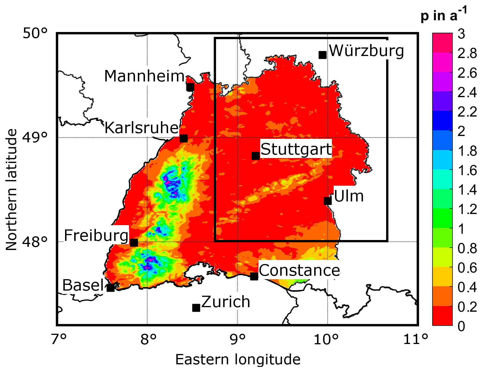
Figure 2Probability of observed 24 h rainfall totals greater than 50 mm, expressed as the average days per year for Baden-Württemberg; the black box indicates the area where background precipitation R∞ is estimated.
2.3 Modifications of the SBM
As further development, two types of modifications are applied to the SBM: adjustments to the existing orographic precipitation using additional calibration parameters and additional precipitation components originating from different physical processes.
2.3.1 Adjustments to Roro
The original orographic precipitation equation of the SBM (Eq. 2) is modified in the SPM2D by adding three constant calibration parameters (bold symbols):
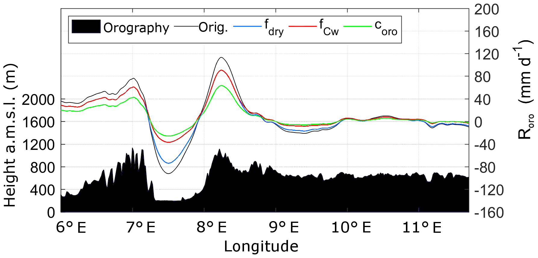
Figure 3Different effects of the implemented internal free parameters fdry (blue), (red), and coro (green) on the original orographic precipitation part (black curve) for a west-to-east cross section through the model domain. The underlying orography is shown in black.
The uplift sensitivity factor Cw is adjusted by a multiplier , which reduces the sensitivity of the SPM2D for lifting and, therefore, the precipitation rate. Precipitation is reduced the most for sharp height gradients, whereas the effect is only weak for smooth terrain (Fig. 3, red curve). The formulation of the SPM2D also allows for multiple ascents and/or descents of a virtual air parcel without any changes in its water vapor content. The more realistic partial removal of water vapor due to condensation during the ascent is also considered by implementing the additional function .
An additional parameter, fdry, is implemented in Eq. (4) to reduce evaporation in descent regions, where Roro becomes negative (Fig. 3, blue curve). The resulting underestimation of precipitation is found especially downstream of steeper mountains with a greater descent (Kunz, 2011). The parameter fdry<1 only corrects grid points (x, y) where Roro<0; otherwise fdry=1.
Finally, the last additional calibration parameter, coro, reduces orographic precipitation in the whole domain (Fig. 3, green curve). It is a consequence of the assumption that the vertical lifting of an air column with overall saturation produces condensate and instantaneous fallout at any time, implying an overestimation of precipitable water. In reality, not all layers are completely saturated, and water may also partly be stored by clouds. The parameter coro is assumed to be independent of any lifting processes and constant in time for the whole domain. From a mathematical perspective, the two factors, and coro, could collapse into one single parameter. Nevertheless, as mentioned above, they describe modifications of different physical processes and must therefore remain separate.
2.3.2 Frontal precipitation
Apart from large-scale lifting connected to low-pressure systems or waves in the flow patterns, precipitation is also substantially enhanced by synoptic-scale weather fronts. Active fronts may increase precipitation considerably due to cross-frontal circulations and lifting in the warm sector of a cyclone (e.g., Bergeron, 1937; Eliassen, 1962). Conversely, if a front affects only parts of the investigation area (e.g., in case of a trailing front, where the flow is almost parallel to the isobars), regions not affected by the front experience much less or even no rain at all. Both effects are considered by a simplified parameterization Rfront in Eq. (1):
where cfront serves as an enhancement or reduction factor of the overall precipitation. In this parameterization, Roro is considered again because frontal precipitation is additionally enhanced by orography, as shown, for example, by Browning et al. (1975) or Houze and Hobbs (1982). Due to the additive superposition of all precipitation components in Eq. (1), we have to subtract the original precipitation totals, leading to a total multiplier of (cfront−1).
In order to estimate cfront from the observational data, we define this quantity as the relative difference between observations O and output M of the SBM. This is expressed by
assuming that the differences originate primarily from frontal effects. For the quantification of cfront, we use spatial mean values over the investigation area and for a training sample of historic heavy rain events (see Sect. 2.4.1).
The frontal enhancement factor is a function of space realized by a rectangular area cfront(n, t), where the orientation of the front-parallel t axis compared to the zonal-orientated y axis is prescribed by the mean wind direction β (Fig. 4). For each time step the maximum value of cfront is estimated using the corresponding PDF (cf. Sect. 5.1). To avoid strong gradients at the borders of the rectangular, we applied Gaussian-shaped smoothing. Along the front-normal n axis, the spread is set to 8σn, where σn is the standard derivation of the normal distribution; in the t direction, the front is infinitely extended (Fig. 4). As the minimum of cfront is zero, Rfront can also attain negative values, leading to a weakening of total precipitation for areas unaffected by a front.
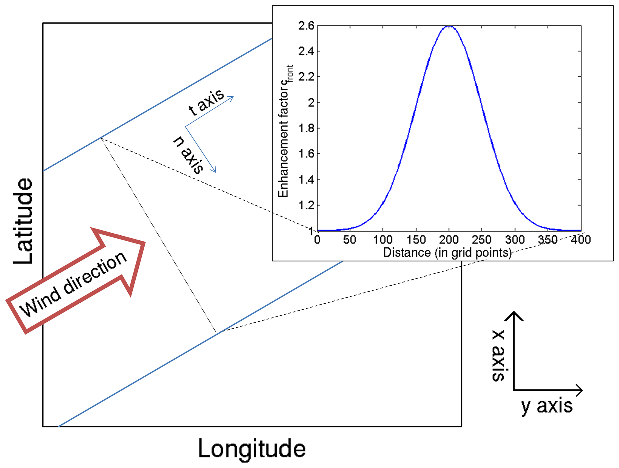
Figure 4Schematic of a Gaussian-shaped distribution of the frontal enhancement factor with a maximum of cfront=2.6 and σn=50 (upper right corner), and its location in the model domain for a southwesterly wind direction (arrow). The blue lines indicate the boundaries of the frontal zone.
2.3.3 Embedded convection
Embedded convection mainly occurs when lifting is locally enhanced at mid- and upper-tropospheric levels, leading to a decrease of thermal stability by the release of latent heat of condensation (e.g., Kirshbaum and Durran, 2004; Kirshbaum and Smith, 2008; Cannon et al., 2012). Convection in general involves several complex processes that make reliable simulations a difficult task. Since our model is restricted to large-scale precipitation with the objective of quantifying extremes of areal precipitation solely, we treat embedded convection in a very simplified way by implementing several rectangular cells as convective footprints, similar to the approach for the fronts.
Because embedded convection is mainly induced by orographic lifting, we implemented a multiplicative factor to the precipitation fields related to both orographic and large-scale lifting, similar to the frontal part:
with the enhancement factor cconv. For each 24-hour simulation period, we choose a number of rectangular convective footprints, each with a specified width W and length L, and distribute them randomly over the whole model domain (Fig. 5). The dimensions for each rectangle are estimated from the PDFs of historic footprints of deep moist convection (see Sect. 3.3). Furthermore, we restricted the two parameters to L>W and Lmax=300 km, or 300 grid points. As for the frontal systems, the wind direction defines the orientation of the longer sides of the rectangles. For each footprint, we choose a number of L⋅W specific factors, cconv, with cconv∈{0; 1}. As found, for example, by Fuhrer and Schär (2005) or Cannon et al. (2012), embedded convection can enhance precipitation up to 200 %, but only locally. Thus, the given range of cconv is adequate. Within the single rectangles, the spatial distribution of cconv randomly varies between the given limits to account for the high spatial variability of convective precipitation.

Figure 5Schematic of embedded convection implementation by using rectangular cells (blue). The orientation is defined by the wind direction (arrow); each cell is assigned to an individual factor cconv.
As embedded convection occurs several times a day and at several locations, we used a variable number of convective footprints in the model. The complete convective precipitation field for each time step is spatially smoothed to avoid sharp gradients. For this, we applied a moving average of 10 grid points to preserve the high spatial variability of convection.
2.4 Pre-preparation and simulation procedure
2.4.1 Event definition and statistical distribution functions
Stochastic modeling of precipitation events with the SPM2D is based on appropriate PDFs of all input parameters required by the model. These PDFs are estimated using an adequate set of representative past heavy rainfall events. Because the characteristics of the ambient conditions and thus the precipitation regimes change throughout the year, we seasonally differentiate the estimated PDFs between spring (March–April–May – hereafter MAM), summer (June–July–August – JJA), autumn (September–October–November – SON), and winter (December–January–February – DJF).
In the first step, a sufficient and appropriate subset of relevant historic events was identified. Here, an event is defined as a period of 1 or more days with persistent precipitation above a certain threshold of daily totals. An extension to multi-day events is reasonable for considering time delays in discharge response or flood waves traveling along river networks (e.g., Duckstein et al., 1993; Uhlemann et al., 2010; Schröter et al., 2015).
We define the historic event set according to maximum areal precipitation. For this, we simply accumulate the (equidistant) 24 h rainfall totals of all grid points in the investigation area (BW; see Sect. 3.1). Following the sorting of all values of in descending order, the strongest 200 values enter the sample (top200). As precipitation is not limited to these (single) days but may be embedded in longer time periods, we define the threshold Rthres for the event definition. For estimating Rthres, we consider “wet” days by using solely and set Rthres to the 75 % percentile of this subsample. A lower threshold leads to an overinterpretation of longer clusters, and a higher one avoids multi-day events.
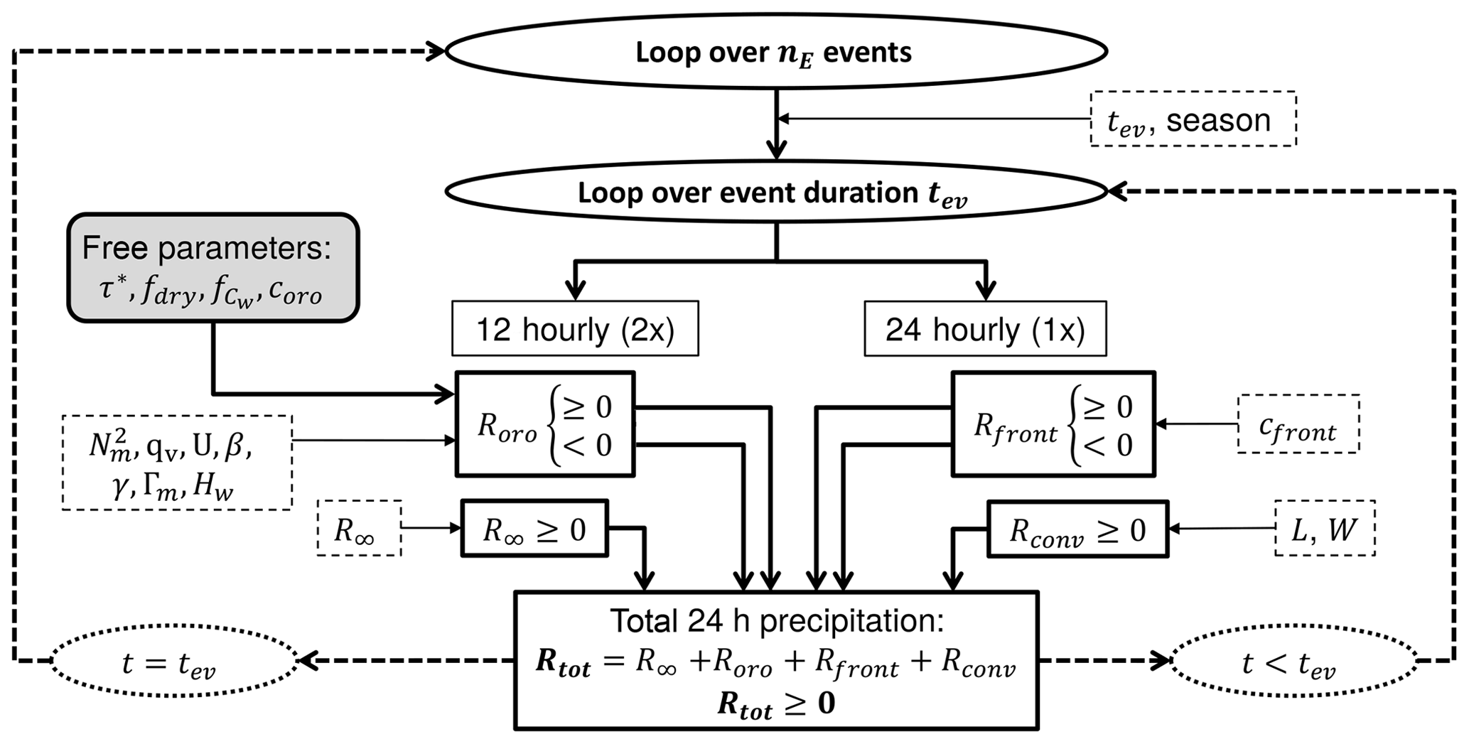
Figure 6Flow chart of the individual components of the SPM2D (solid boxes) and the corresponding input variables (PDFs; dashed boxes). Loops are highlighted as ellipsis or bold dashed arrows. The constant model parameters are illustrated as the shaded box.
Event precipitation starts on the first day that exceeds Rthres. When areal means of consecutive days are also above Rthres, they are simply accumulated, yielding events of more than 1 day. The last day with R≥Rthres before a period of at least 3 three days of non-exceedance defines the end of an event. Such a 3-day period ensures statistical independence of the events in accordance with the approach of Palutikov et al. (1999) for wind storms. Following Piper et al. (2016), we only count “rain days” () and neglect “skip days” () within the start-day and end-day period for event duration estimation, which is a widely used approach (Wanner et al., 1997; Petrow et al., 2009). This approach avoids the overinterpretation of longer clusters. Based on this procedure, a defined precipitation event contains 1 or more days of the top200 sample. For this event set, all required input parameters were extracted from sounding data and rainfall totals (see Sect. 3).
In the next step, we identified the PDFs most appropriate for statistically describing each of the seven atmospheric input parameters, the event duration tev, background precipitation R∞, and front factor cfront. In addition to 20 PDFs preset by the MATLAB statistical toolbox (MATLAB, 2016), we considered the circular von Mises distribution (Mardia and Zemroch, 1975) for wind direction only. In Sect. 5 it will be further discussed which PDFs are most suitable for the input variables in our case.
To find the PDF that best fits the data, we estimated the appropriate number of histogram classes according to Freedman and Diaconis (1981) and calculated bias, the root-mean-square error (RMSE), and the Spearman correlation coefficient rSp (Spearman, 1904) as quality indicators (QIs). We also applied a χ2 test (Wilks, 2006) as a QI. For each QI, we ranked the PDFs in ascending order and added up the rank numbers for each PDF, receiving the best fit in terms of the least QI rank sum (QIRS). In the case of alikeness of two or more PDFs (about 10 % of all cases), we manually selected the best one.
2.4.2 General simulation procedure
The presented SPM2D is an event-based model in the sense that a specified number nE of independent events with variable duration tev is simulated. The general procedure is as follows (cf. Fig. 6). Starting with the iteration loop over nE events, the season and duration tev are set at first. The next step is the simulation of the four precipitation components according to Eq. (1); because radio soundings used as input data are available every 12 h, Roro and R∞ are computed for the same period. In contrast, Rfront and Rconv are calculated only for 24 h as they become apparent as footprints in daily totals. The resulting total precipitation Rtot has a temporal resolution of 24 h. Despite the fact that the characteristic timescales may vary from one situation to another, it is found that simulations using fixed values for the free parameters yield trustworthy results (e.g. Barstad and Smith, 2005; Kunz, 2011). Here, we also use constant values illustrated as the shaded box in Fig. 6. The direct link between the precipitation components and the corresponding input variables (described by appropriate PDFs) is also shown in Fig. 6. In case t<tev, the next 24 h period is simulated; otherwise, the loop jumps to the next event. A method how to assign the nE events to a specific time period, which is required, for example, for insurance purposes, will be introduced in Sect. 6.
The SPM2D presented in this study is based on two different types of data sets: gridded precipitation data also used to calibrate and verify the model and vertical profiles from radiosondes to initialize the model. Furthermore, the SPM2D is also validated using reanalysis.
3.1 Rainfall totals
Rainfall statistics in our study are based on the regionalized precipitation (REGNIE) data provided by the German Weather Service (DWD). REGNIE is a gridded data set of 24 h totals (06:00 to 06:00 UTC) based on several thousand climate stations more or less evenly distributed across Germany (so-called RR collective). The REGNIE algorithm interpolates the observations to a regular grid of 1 km2 considering elevation, exposition, and climatology (Rauthe et al., 2013). Despite of continuous changes in the number of stations considered and several station relocations, REGNIE is sufficiently homogeneous for our purposes. However, areal precipitation exhibits a certain bias, especially over elevated terrain, such as the peaks of the Black Forest, where the number of stations is very limited (Kunz, 2011).
In our study, we use REGNIE data from 1951 to 2016 to identify the top200 event set (see previous section); to estimate the duration of the events, the front factor cfront, and background precipitation; and to validate the SPM2D simulation results.
3.2 Radio soundings
The seven input parameters (see Sect. 2) required by the SPM2D model are derived from vertical profiles (00:00 and 12:00 UTC) of temperature, moisture, wind speed, and direction at the radio sounding station of Stuttgart located somewhat downstream of the northern Black Forest. Even though the location might not be ideal because the profiles do not represent undisturbed conditions, the profiles are similar to those of the upstream station of Nancy in France, as shown by Kunz (2011) for heavy rainfall events on average. Data from Nancy are available after 1990 only and, thus, cannot be used in this study, whereas soundings from Stuttgart have been available since 1957.
The vertical profiles, provided by the Integrated Global Radiosonde Archive (IGRA) from the National Climatic Data Center (Durre et al., 2006), were interpolated into equidistant increments of Δz=10 m (Mohr and Kunz, 2013). All derived environmental parameters refer to the lowest 5 km of the atmosphere since this layer is most relevant for airflow and stability. Furthermore, to account for the decreasing impact of higher atmospheric layers on the flow characteristics, the flow parameters Λ are integrated vertically (), applying water vapor weighting (Kunz, 2011):
where ρd is the density of dry air and zt is the upper integration limit, here of 5000 m. As some layers may be moist-unstable, resulting in imaginary Nm, the averaging routine is applied to . In the few cases where was imaginary, it was set to a near-neutral, constant value of 0.0003 s−1.
3.3 Parameters for embedded convection
The stochastic generation of enhanced precipitation streaks associated with embedded convection, namely their length and width (L and W), relies on the statistics of severe convective storms in Germany (Fluck, 2018). In that study, convective storms in Germany, France, Belgium, and Luxembourg between 2005 and 2014 were identified from the constant altitude plan position indicator (CAPPI) for a reflectivity in excess of 55 dBZ. The application of the tracking algorithm TRACE3D (Handwerker, 2002) identified more than 25 000 storm tracks. Even though we do not consider rainfall related to severe convective storms in the SPM2D, the statistical distributions of the storm's dimensions are reliable proxies for the extension of enhanced precipitation from embedded convection described by Rconv.
3.4 Numerical weather simulations
The SPM2D simulation results are additionally validated with high-resolution reanalysis from the non-hydrostatic Consortium for Small-scale Modeling (COSMO) model in climate mode (CCLM; Rockel et al., 2008). Natalie Laube (Institute of Meteorology and Climate Research, Karlsruhe Insitute of Technology, personal communication, 2018) performed a dynamical downscaling of an ERA-40 reanalysis from the European Centre for Medium-Range Weather Forecasts (ECMWF; Kållberg et al., 2004) to a horizontal resolution of 2.8 km for southern Germany using a 3-fold regional nesting (50 km, over 7 km, to 2.8 km). High-resolution CCLM data are available for the period 1971–2000. For the evaluation, we considered the top200 REGNIE events from which around 100 events occurred within the CCLM period, including the top two events, seven of the strongest 10 events or 14 of the strongest 20 events.
4.1 Method
The SPM2D is calibrated with the top200 events (training data) by adjusting the free model parameters τx, , fdry, and coro (cf. Sect. 2) and comparing the simulation results with observations. The parameter combination yielding the best simulation results is then used for the stochastic simulations (validation data). The components Rfront and Rconv are only considered for the stochastic event set and are therefore neglected here. In this configuration, the SPM2D is equivalent to the SBM plus our modifications in Roro, referred to as the SBM + M.
In order to determine appropriate values of the free parameters, a large number of model simulations were carried out. Whereas one parameter was successively varied, the others were kept constant. The selected ranges and increments of the parameters listed in Table 1 resulted in 2016 possible parameter combinations, giving a total number of approximately 390 000 simulation days for the top200 event set. Both data sets (from SBM + M and REGNIE) are slightly smoothed using a running 5×5 grid box, as the REGNIE data show a certain spatial uncertainty (cf. Sect. 3.1), especially around the crests of the Black Forest. Furthermore, as shown, for example, by Barstad and Smith (2005), smoothed data yield more robust results when comparing model and observation data. Note, however, that larger values of τx and smaller values of similarly smooth the simulated precipitation fields. In these cases, the QIRS method used for the evaluation (Sect. 2.4.1) has to be applied carefully.
Table 1Range of values of the free model parameters used for the calibration of the model.

The model skill was evaluated using the skill score S according to Taylor (2001) (see Eq. A1 in the Appendix) to determine the best combination of the free model parameter. S relies on the Spearman (1904) correlation coefficient rSp between the SBM + M simulations and the observations (REGNIE) as well as on the standard deviations σ of both data sets. The skill score S is computed for each day of the top200 and each parameter combination. From all realizations, we select the parameter combination that yields the highest median value of S averaged over the top200, as the SPM2D should be able to properly represent a broad range of different atmospheric conditions.
4.2 Calibration results
Applying the method as described above, the highest value for S=0.60 as the median of all top200 events is obtained for the combination of τx=1400 s, , fdry=0.4, and coro=0.8. For this combination, the median values of the other quality indices are rSp=0.39, , bias = 6.30 mm, and RMSE = 14.85 mm. The assessed value for τx is physically plausible and comparable to other studies with the SBM (e.g., Barstad and Smith, 2005; Caroletti and Barstad, 2010; Kunz, 2011). Considering the slight overestimation of orographic precipitation and the strong overestimation of drying in the lee of the mountains by the SBM, the values for those adjustments are also physically plausible. Note that the parameter combination identified above yields the lowest errors only when averaging over all top200 events. Single events are more realistic with another parameter combination, reflecting particularly the unknown, and thus not considered microphysical processes that are decisive for precipitation formation strongly controlled by vertical wind speed, temperature, and moisture profiles. The dependency of microphysical processes on ambient conditions, however, is not relevant when running the model in the stochastic mode, which is the objective in this study.
The sensitivity of the skill score S to changes in τ, , and coro (Fig. S1 in the Supplement) shows a kind of dipole structure in both cases with the highest values of S along the counter diagonal. Lower values for S are obtained for the shortest (longest) timescales in combination with the highest (lowest) uplift sensitivity or highest (lowest) weighting of Roro in Eq. (1). This means that horizontal precipitation drift over short distances also reduces evaporation, leading to an overestimation of orographic precipitation (and vice versa). This effect has to be considered by adjusting Roro.
4.3 Sensitivity of simulated total precipitation
To demonstrate how variations of atmospheric conditions translate into precipitation, we conduct a sensitivity study with the SBM + M using the top200 event set by gradually changing the values of the input parameters. Following Kunz (2011), we perturbed the values of , qv, U, β, and τ. This is done by multiplying the respective quantity with var_mult increasing linearly from 0.5 to 2.0 in increments of 0.1. Wind direction β is varied in the range of ±30∘ in increments of 5∘. The calibration parameters are set to their optimum values estimated in the previous section. Besides areal mean precipitation, we computed RMSE and skill score S for the median of the top200 event set.
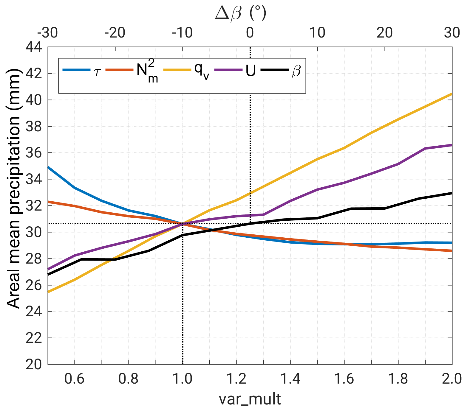
Figure 7Areal mean precipitation (24 h totals; median of the top200 event set) as a function of , qv, U, β, and τ, perturbed by a multiplicative factor () and changed Δβ. The dotted lines indicate the values of the reference run.
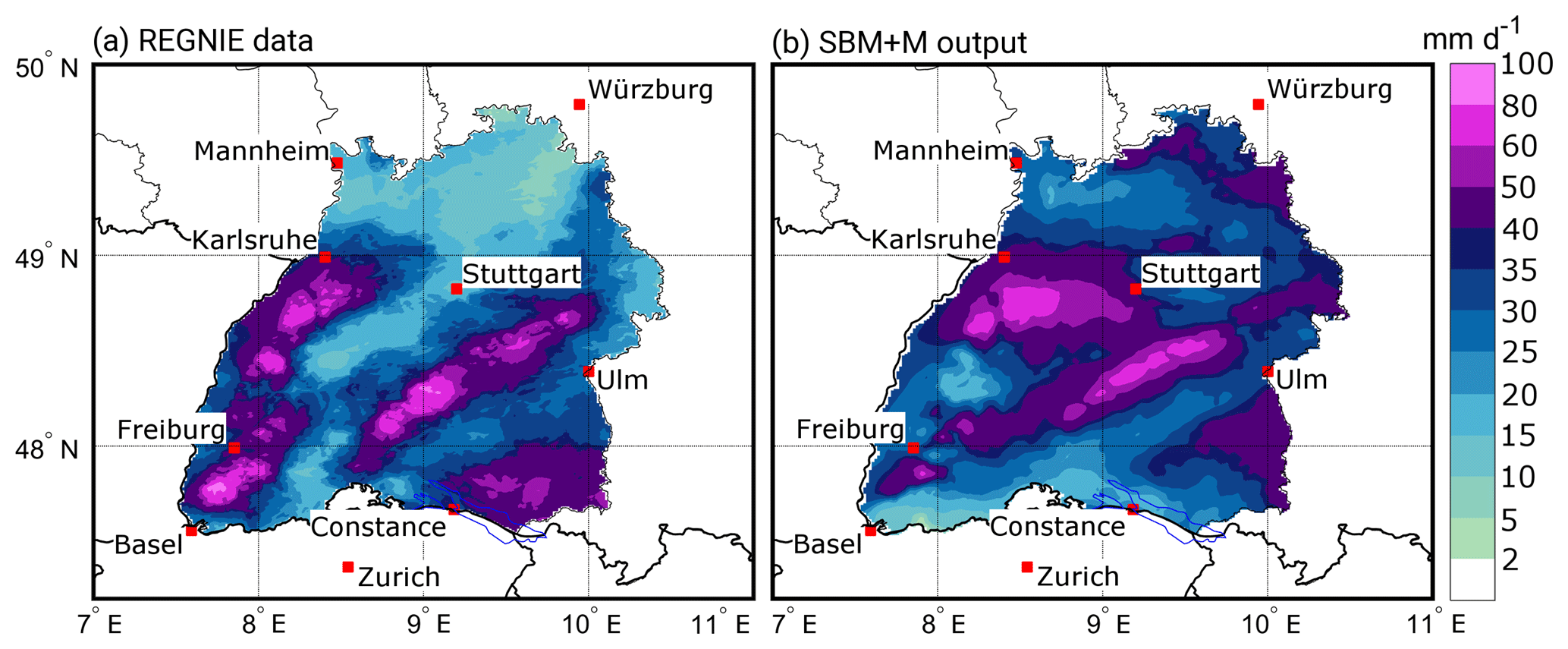
Figure 8Comparison of (a) REGNIE 24 h rainfall totals, and (b) SBM + M output for southwestern Germany for the case study on 31 May 2013. Note that REGNIE data are available for Germany only. The parameterization in (b) is τx=1400 s, , fdry=0.4, and coro=0.8. The areas outside of Baden-Württemberg are white for better visualization and comparison.
Mean precipitation shows a high sensitivity to changes in qv, U, and β (Fig. 7). In all cases, precipitation increases with increasing values and decreases with decreasing values. Lowest sensitivity occurs for β between ±15∘ because of the orientation of the major orographic structures (i.e., the Black Forest) from southwest to northeast. Westerly inflow, prevailing on average, still occurs for small variations of β. For greater shifts (Δβ>20∘ or ∘), when the inflow angle becomes smaller, the sensitivity slightly increases. The changes in the wave regimes, and thus the location of the updraft, may also explain the partly stepwise form of the curves for both β and U. The results for and τ reveal the opposite behavior with an increase in precipitation for smaller values and vice versa. Furthermore, the sensitivity of the SBM + M to changes in these two parameters is much weaker compared to the other parameters.
Qualitatively similar behavior to the model is found for the medians of RMSE and skill score S (Fig. S2). While areal precipitation only provides insights into how changes in the ambient parameters feed back into rainfall, RMSE and S also consider the spatial distribution. The results for RMSE (Fig. S2a) again reveal the highest sensitivity of the SBM + M to changes in qv and U. While for var_mult > 1, the sensitivity in terms of RMSE is similar to areal precipitation, there is a much higher sensitivity for var_mult < 1. In those cases, orographic precipitation is more detached to the mountain crests, resulting in higher totals due to reduced evaporation in the descent regions. Because of the combination of higher totals at different locations, RMSE shows a higher sensitivity to changes in τ and compared to areal mean precipitation.
The skill score S, in contrast, is most sensitive to changes in qv and τ (Fig. S2b). Regarding , S decreases just for very high values of var_mult, while there is almost no sensitivity on β. In all cases, highest S is obtained for the original values of the input parameters, confirming that the model is well calibrated.
4.4 Case study
After the parameter adjustment, the SBM + M tends to slightly underestimate orographic precipitation, whereas totals over flat or rolling terrain are overestimated. This behavior can be seen for the case study of 31 May 2013 (Fig. 8), a heavy precipitation event that triggered the severe flooding in 2013 (Schröter et al., 2015).
On that day, a pronounced low-pressure system with its center over Croatia led to the sustained advection of moist air masses from northerly directions around 20∘ in combination with a synoptic-scale ascent. The Stuttgart sounding showed low stability (Nm=0.0055 s−1), high precipitable water (pw = 24 kg m−2), and high wind speed (U=20 m s−1), which is already an indication of heavy rainfall. Consequently, precipitation totals across the investigation area reached values of 10–100 mm.
Overall, the SBM + M is able to reproduce most of the structures of the observed rain field (Fig. 8), especially the location of the maxima. The observed mean for Baden-Württemberg is mm, whereas the simulated mean is mm, thus being only 12.6 % higher compared to the observations. Maximum values are mm and mm, which is a deviation of about 17 %. The area with R≥50 mm is almost equal with slightly less grid points (≈6 %) in the SBM + M. The best agreement is found for the northern Black Forest as well as the Swabian Jura. Over the northern part of the model domain (north of 49∘ N) and southwest of Stuttgart, simulated rainfall is substantially higher compared with REGNIE. In contrast, the SBM + M simulates lower totals in the southern Rhine Valley near and over the mountainous regions of the southern Black Forest (around Freiburg), especially east of the city of Basel, where lee-side evaporation in the model dominates. The quality indices for that day are S=0.62, rSp=0.30, , bias = 4.44 mm, and RMSE = 14.82 mm.
One reason for the discrepancy between observed and simulated precipitation might be the suboptimal location of the Stuttgart sounding used for the model initialization. The sensitivity study as described in Sect. 4.3 for this particular event obtains the best results in terms of the lowest RMSE (Fig. 9) for an increase in or τ, whereas in the case of qv or U, the lowest RMSE is obtained when decreasing the original values. Regarding β, the lowest RMSE is given for the original value. The highest skill score S, conversely, is reached for increasing U and qv and decreasing τ and . In the case of β, S continuously decreases from 0.8 for northwesterly inflow to 0.4 for northeasterly winds.

Figure 9Changes in (a) RMSE, and (b) skill score S for perturbed values of , qv, U, β, and τ, with a multiplicative factor (var_mult), and changed Δβ, for 31 May 2013. The dotted lines indicate the values of the reference run.
5.1 Adjustment of the PDFs
After separating the historic event set into the four main seasons, we estimate, for each of the 10 input parameters, the PDF that best fits the distribution of the observations (Table 2) by using the least QIRS method (cf. Sect. 2.4.1). From the overall 21 PDFs that were considered, only 12 turned out to be suitable for adjusting the observations. In most of the cases, the generalized extreme value distribution (GEV), with its special realizations of the Gumbel distribution (GbD) and Weibull distribution (WbD), appears to be appropriate (26 cases), followed by the inverse Gaussian distribution (IGD) for five parameters and the Gamma distribution (GmD) for three parameters. Especially for flow parameters derived from the soundings, the GEV appears to be the most appropriate (19 out of 28 cases). We had to choose the PDF manually 5 times due to the alikeness of two PDFs according to the QIRS method.
Table 2Estimated best-fitting PDFs for event duration (tev), background precipitation R∞, and frontal enhancement factor cfront derived from REGNIE data (top box); square of saturated Brunt–Väisälä frequency , wind direction β, horizontal wind speed U, scaling height Hw, actual lapse rate γ, saturated moist adiabatic lapse rate Γm, and condensation rate derived from sounding data (bottom box). For the PDF acronyms, see Table A1.

The input parameters are considered as independent and uncorrelated. To justify this assumption, we performed a correlation analysis of all possible combinations of input parameters using the Spearman (1904) correlation coefficient. A low number of about 16 % of the parameters have a correlation coefficient above ±0.5, and only 4 % are highly correlated with ±0.7. Regarding these cases, 90 % show negative correlations with . However, there are distinct seasonal differences; in some cases correlations are higher in summer than in winter. The highest correlation exists between and the lapse rates, which is plausible as both are based on the vertical temperature gradient. Because the SPM2D is less sensitive to (cf. Sect. 4) the effect can be neglected in the model.
5.2 Event characteristics
The histogram of the duration tev for the top200 event set and the corresponding best-fitting PDF, shown exemplary in Fig. 10, illustrated that during JJA, a duration of 2–3 days dominates, with a decreasing probability toward longer periods. During DJF, the distribution is generally shifted to longer events, whereas the probability for single-day events remains roughly unchanged. The maximum of 15 days in DJF represents the longest duration of the top200 event set. Whereas the estimated PDF for the JJA (GEV) has a sharper maximum and a stronger decrease in tev>3, the PDF found to best fit the duration in the DJF (NkD) shows a broader range of possible durations. Note that the histogram in the winter shows a large scattering with irregular peaks, making an adjustment of a PDF difficult. For MAM and SON, the results are comparable to those of DJF and JJA, respectively.
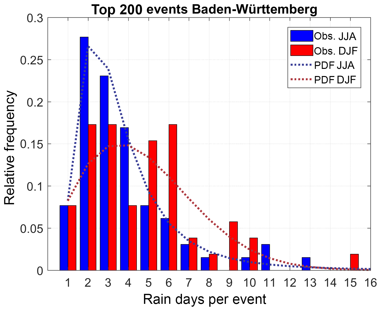
Figure 10Histogram of top200 event duration for Baden-Württemberg according to REGNIE (bars), and estimated best-fitting PDFs (dotted lines) for the summer (blue) and the winter (red).
Concerning R∞, totals of 20–25 mm day−1 are found to most likely occur within a range of 3–37 mm day−1 in DJF, 3–50 mm day−1 in JJA, and 0–50 mm day−1 during the other two seasons (not shown). The corresponding PDFs are listed in Table 2. For the cfront parameter, all PDFs have their maximum around 0.7 to 0.8, with a range from 0.4 to 1.4 for most of the seasons (not shown). The distribution in SON (Table 2) descends slower towards higher values (maximum of around 1.6).
5.3 Atmospheric parameters
An overview of the range of the seven input parameters of the model is shown as box plots in Fig. 11; the corresponding PDFs are listed in the bottom box of Table 2. In most cases, the atmosphere was slightly stably stratified, as represented by positive values of affecting the wave propagation. During JJA, the distribution is shifted toward negative values (unstable; recall that negative values are set to Nm=0.0003 s−1), whereas in DJF, there are almost entirely positive values. Wind direction β, decisive for the spatial distribution of precipitation around the mountains, shows pronounced seasonal differences. More than 90 % of the top200 DJF events have southwesterly to northwesterly winds (240–300∘), with other directions hardly observed. The reason is that northerly flows are usually associated with low temperatures and thus low humidity during DJF. In JJA, the wind direction that occurred most frequently is between 240 and 300∘ as well. However, all other directions have been observed as well.

Figure 11Atmospheric parameters required as input for the SPM2D derived from radio sounding observations at Stuttgart for the top200 events with mean, interquartile distance, minimum, and maximum values; the left whisker of each pair represents the summer, and the right one represents the winter season. The units for each variable are given in the brackets below the variable names.
Horizontal wind speed U in all cases and all seasons is high, especially during DJF, where reduced moisture is compensated by high velocity to obtain substantial horizontal incoming moisture flow. Median values are 5 and 20 m s−1 during JJA and DJF, respectively. Flow parameters related to humidity (Hw, ) conversely show higher values in JJA, where Γm is reduced due to the release of latent heat. The quantity γ shows similar medians and interquartile ranges with a broader distribution in DJF.

Figure 12Precipitation fields for the median of (a) the top200 (REGNIE) events, (b) the SBM + M part of the stochastic events, (c) the full SPM2D stochastic event set, and (d) the CCLM simulations of the top REGNIE events.
Overall, a total number of nE=10 000 events (equivalent to approx. 31 500 days) have been simulated with the SPM2D in stochastic mode (see Sect. 2.4.2). Therefore, a stochastic set of input variables with the same size as the number of simulation days was created using the estimated PDFs, where the variables can be treated as independent (cf. Sect. 5.1). For the validation of the SPM2D, we quantified statistical metrics such as return periods, probabilities, and percentiles and evaluated them with observations (REGNIE), CCLM simulations, and the SBM + M part. The statistical distribution of the stochastic event set of the SPM2D should agree with that of the top200 historic events to a large degree, and more robust results should be notable at the heavy tail (extreme events). The comparison with the SBM + M part is helpful in highlighting the quality and necessity of the modifications made to the original SBM. High-resolution CCLM simulations are chosen for validation to demonstrate the advantages of using a statistical approach for stochastic simulations instead of a dynamical NWP model.
Spatial 24 h mean values range between 1.2 and 79.7 mm in the SPM2D, and 1.3 to 97.0 mm in the SBM + M, whereas the maximum for the top200 is only 49.6 mm. In total, 128 events (0.4 %) of the SPM2D or 724 (2.1 %) of the SBM + M yield higher spatial precipitation amounts than the maximum of the top200. The CCLM simulations range between 1.8 and 37.6 mm.
Both the median and the 90th-percentile (p90) precipitation fields of the top200 event set and the SPM2D agree well concerning the spatial distribution and the precipitation amounts (Figs. 12 and 13). Significant orographic precipitation enhancement over the Black Forest and Swabian Jura is clearly visible in all data sets. Note that the more detailed structure of the REGNIE data results from the regionalization method and its strong dependency on orography, which should not be overinterpreted. Larger spatial differences between the different realizations mainly appear in the northern Rhine Valley and to the northeast of the domain for both the median and the p90, whereas for the latter, some differences also arise northeast and southwest of Stuttgart. Nevertheless, all differences are small, of the order of a few percent. The SBM + M shows an overestimation of precipitation over mountainous terrain, while the CCLM simulates less precipitation overall for the median. For the p90, major differences appear especially over the rolling terrain.
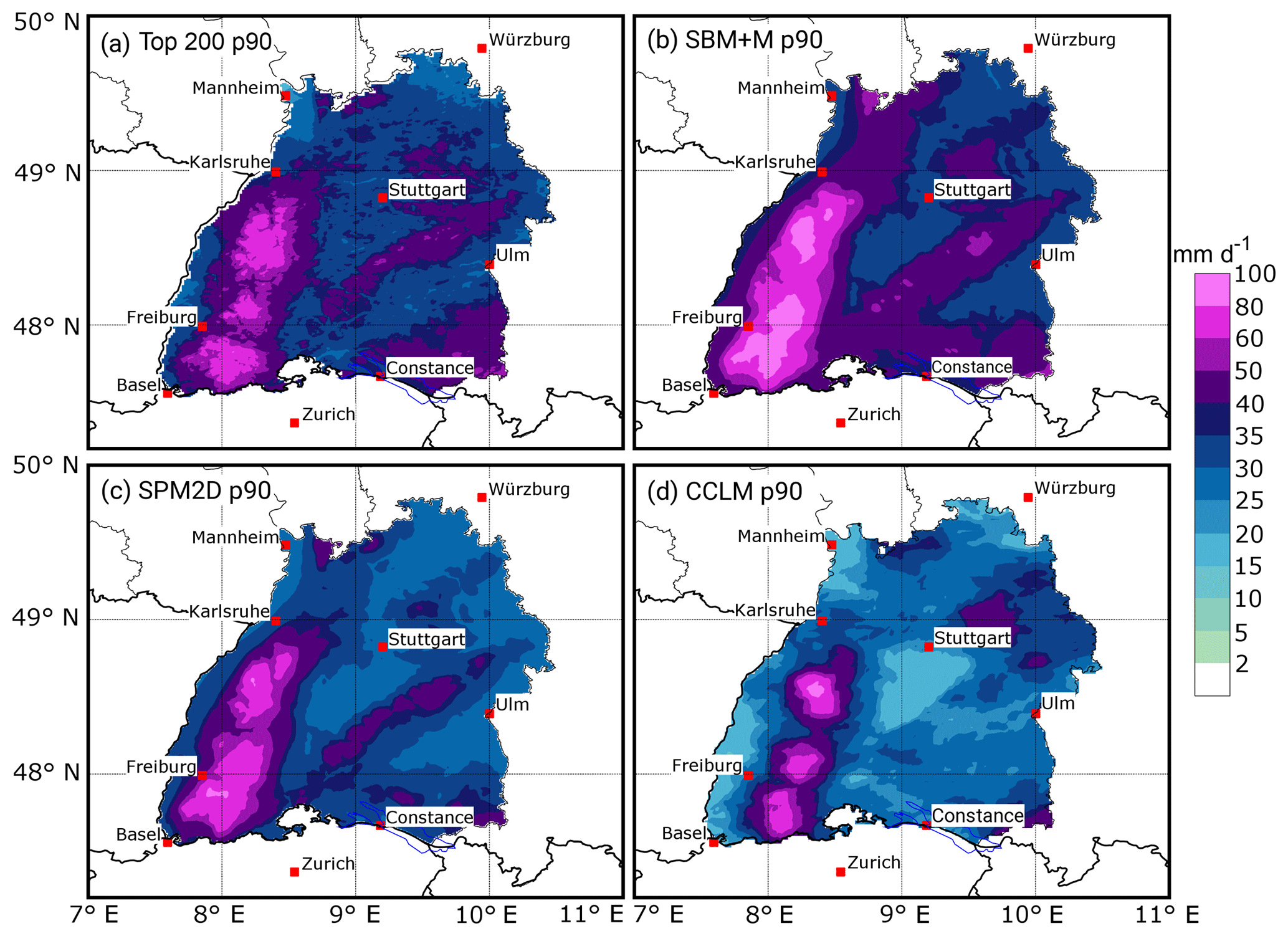
Figure 13Precipitation fields for the 90th percentile (p90) of (a) the top200 (REGNIE) events, (b) the SBM + M part of the stochastic events, (c) the full SPM2D stochastic event set, and (d) the CCLM simulations of the top REGNIE events.
The areal rainfall of the SPM2D median (Fig. 12) differs only about 3.3 % from the REGNIE top200, whereas that of the SBM + M is about 22.1 % higher. The spatial mean of the CCLM reanalysis is around half of REGNIE, which might be a result of the reduced sample size. The maximum values at any grid point of the median field are about 7 % higher in the SPM2D compared to the REGNIE top200, and are about 34 % higher in the SBM + M realization, whereas the CCLM maximum is about 44 % smaller.
The areal rainfall for the p90 field (Fig. 13) is about 6.5 % smaller in the SPM2D and about 14 % higher in the SBM + M, but it is about 22 % smaller in the CCLM. The maximum values at any grid point of the p90 field are approximately 1 % smaller in the SPM2D, about 22 % higher in the SBM + M, and 13 % higher in the CCLM.
For other percentiles the differences between REGNIE and the SPM2D are very small for both the spatial mean and the maximum precipitation at any grid point in the model domain (Fig. S3a). The differences become considerable only above the 95th percentile. The SPM2D tends to overestimate lower precipitation amounts because the minimum values at any grid point are higher in the model than in the observations and invert for the 99th percentile only. In contrast, the differences between the SBM + M and REGNIE are considerably larger for maxima, minima, and spatial means throughout every percentile. The CCLM reanalysis has a negative deviation for minimum and spatial mean precipitation at all percentiles, whereas for the maximum values there is a marked underestimation for lower percentiles and an overestimation at higher percentiles. At small percentiles, the QIs, such as rSp, S, or , have low values due to the overestimation of the SPM2D (Fig. S3b). The highest skill is reached around the 90th percentile, with a slight decrease for higher values, which can be the result of the increasing uncertainties of the observations. Nevertheless, a skill score of around or above 0.8 confirms the reliability of the stochastic simulations.
To estimate precipitation distributions for specific return periods, we fit a Gumbel PDF to the annual maximum series of both REGNIE and the SPM2D. As it is not possible to directly estimate the time period and a corresponding annual maximum series for the stochastic event set, we count the number of stochastic values exceeding the 99th percentile of observations and normalize it by the probability of occurrence p99, yielding the new time period:
After sorting the SPM2D realizations in descending order, we take the first nT=TSPM values as the annual series of the SPM2D and estimate a new Gumbel distribution. Using these distributions, we obtain precipitation values for specific return periods for both REGNIE and the SPM2D. This method is applied to both the spatial mean values of different areas and for every single grid point.
For a 10-year return period, the SPM2D shows only small differences in REGNIE of less than ±10 % over almost the entire area; only in a small region in the southern Black Forest is precipitation higher (Fig. 14a). The areal mean difference is only 0.6 %. In the case of T=200 years (Fig. 14b), the slight overestimation in the southern Black Forest area remains almost the same. For this return period, the SPM2D tends to underestimate precipitation, especially in the northern part of BW and in the southeast around Lake Constance. Nevertheless, the differences for most of the grid points are between ±20 %; areal mean difference is about −10 %. Taking into account the increasing statistical uncertainty for higher return periods, this is still a reasonable result.
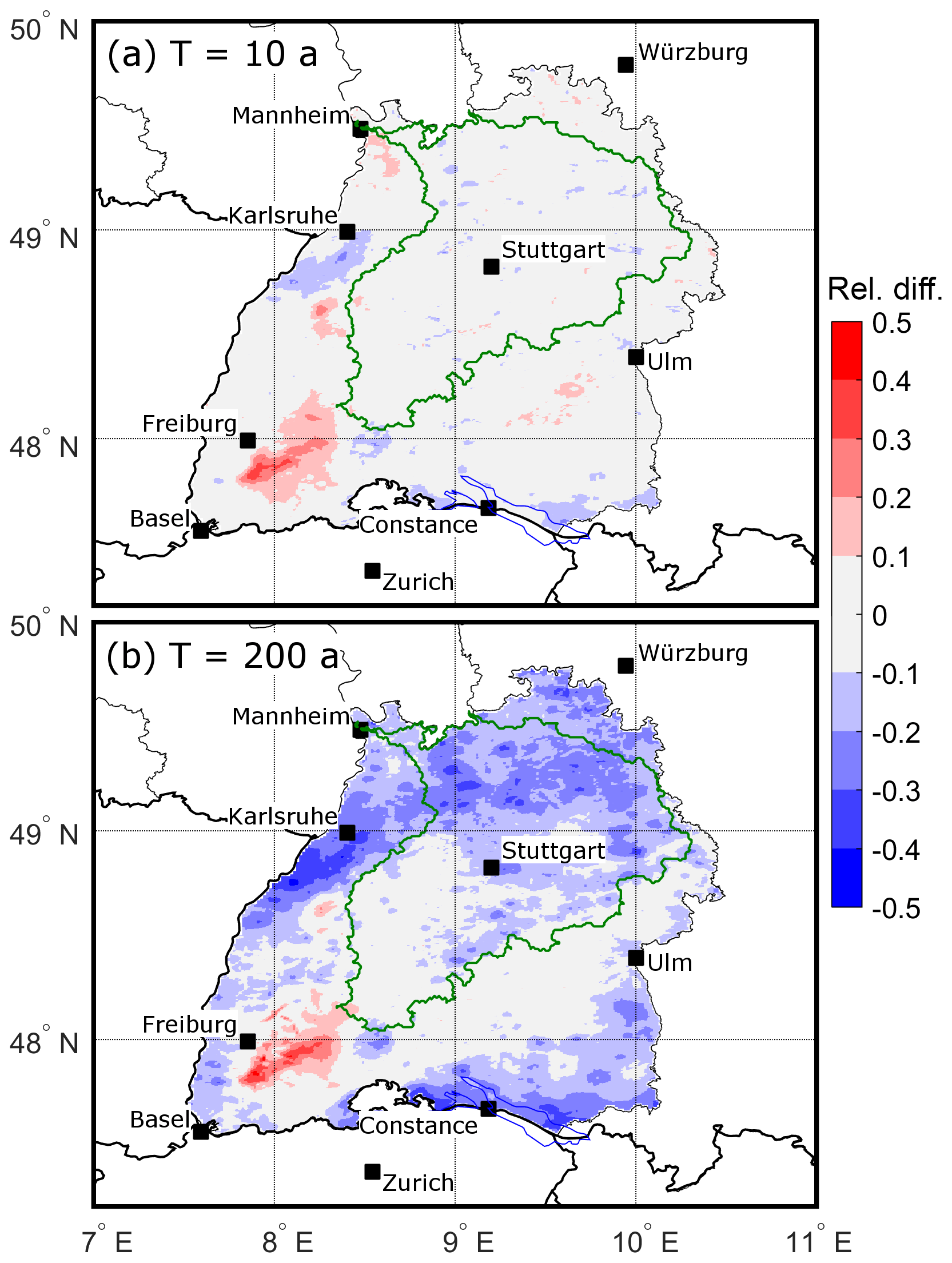
Figure 14Relative difference of the precipitation amounts for return periods of (a) T=10 years, and (b) T=200 years, according to a Gumbel distribution fitted to the observations (top200) and the SPM2D (see text for further explanation). The Neckar catchment is shown as green contour.
On the level of the major river catchments, the differences are small, too. For the Neckar catchment, for example (Fig. 14), which covers about 38 % of BW, the spatial mean deviation is about −0.5 % for T=10 years and −12.7 % for the 200-year return period. Even for catchments containing the area of overestimation in the southern Black Forest, the spatial mean deviations are between +1 and +4 % for T=10 years and between −2 and −10 % for T=200 years.
Single grid point deviations and the ensuing spatial mean values as described above are sensitive to local conditions and uncertainties in both REGNIE and the SPM2D. Hence, we evaluate the model in a similar way by calculating spatial mean precipitation first and then estimating the corresponding return periods (see Appendix A3). Again, the difference between the SPM2D and REGNIE is small for entire BW, with slightly lower values from the simulations (Fig. 15a). The distribution of the SPM2D is very close and almost parallel to the estimated observed Gumbel distribution and within the 95 % confidence interval (CI95) estimated with the formula of Maity (2018). Considerable differences between the SPM2D and REGNIE arise only for return periods of T=1000 years and above but are still small. For the Neckar catchment, the SPM2D agrees well with the observed distribution for return periods up to T=300 years (Fig. 15b). For higher return periods, the differences increase but are still inside the CI95. Similar results can be found for other river catchments (not shown).
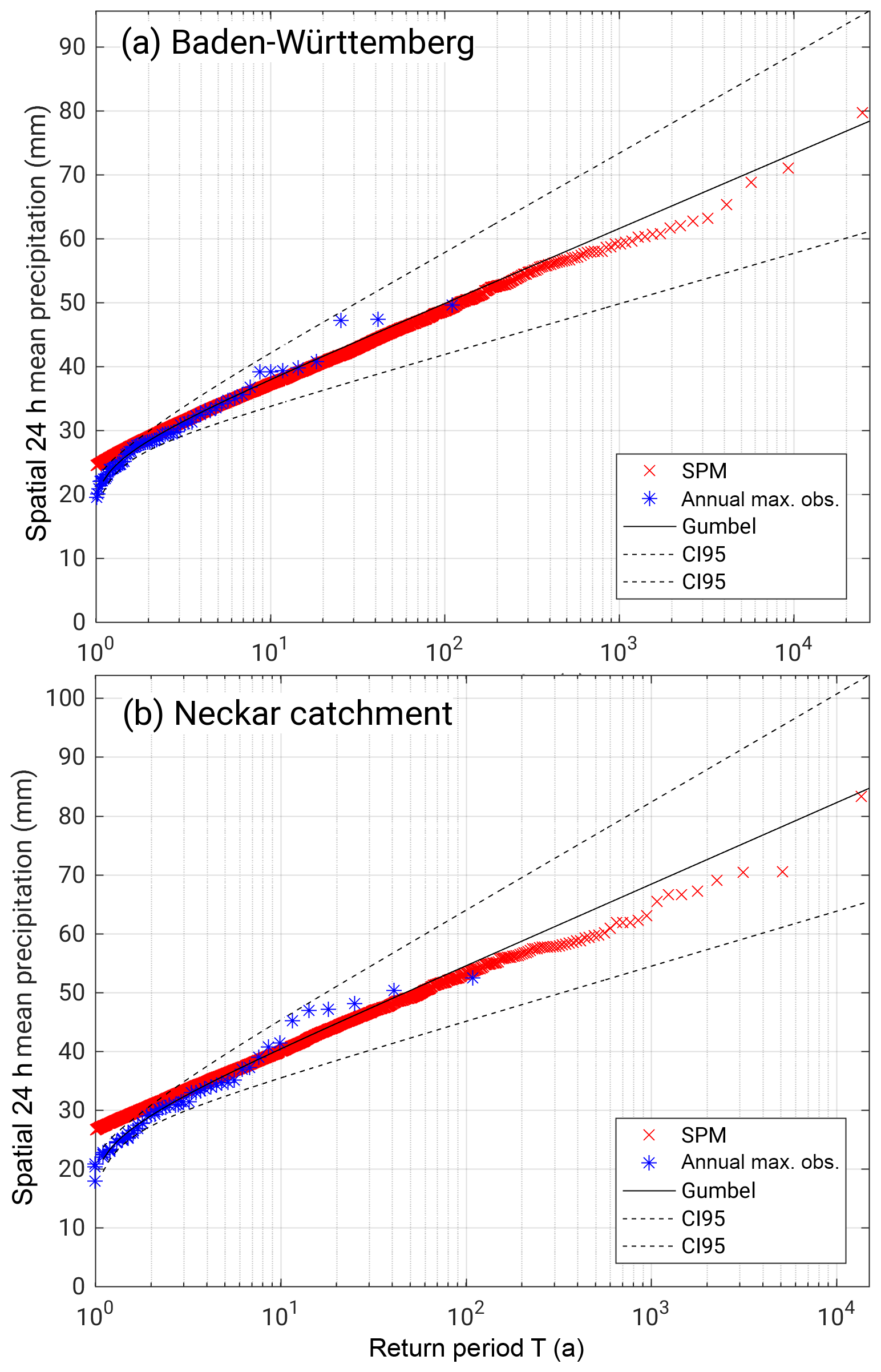
Figure 15Daily rainfall totals (areal means) as a function of return period T based on the annual maximum series of observations (REGNIE, blue), the corresponding Gumbel distribution including the 95 % confidence intervals (black), and the annual SPM2D series (red) for (a) the federal state of Baden-Württemberg and (b) the Neckar catchment.
We have presented a novel method for estimating the statistics of heavy rainfall based on a stochastic model approach. Total precipitation is calculated from the linear superposition of four different parts: orographic precipitation, synoptic background precipitation, frontal precipitation, and precipitation from convection embedded into mainly stratiform clouds. The linear theory of orographic precipitation according to Smith and Barstad (2004), which represents the core of the SPM2D, has been modified using three different calibration parameters to minimize the weaknesses found in previous studies such as the overestimation of wave dynamics and, thus, resulting precipitation and evaporation (e.g., Barstad and Smith, 2005; Kunz, 2011). Furthermore, linear theory gives a physically based linkage of the single grid cells within the model domain, which is an improvement compared to other stochastic weather generators based on pure statistics like those of, for instance, Peleg et al. (2017), Benoit et al. (2018), or Singer et al. (2018). The resulting precipitation fields and statistics are more robust and physically justified. For cross-validation, we calibrated and adjusted the SPM2D to a historic event set of heavy rainfall events (top200; training data). By adjusting appropriate PDFs for all required model parameters, we simulated 10 000 independent stochastic precipitation events (validation data). The results were compared with observations and reanalysis data using different percentiles and return periods.
The focus of the presented investigations was on the federal state of Baden-Württemberg in southwestern Germany, with the striking low mountain ranges of the Black Forest and Swabian Jura. The following main conclusions can be drawn:
-
The SPM2D has high skill for simulating both historic and stochastic heavy rainfall events. The simulated precipitation fields and magnitudes are reliable despite the simplified approach of the model initialized by a set of atmospheric variables obtained from radio soundings. The differences between the SPM2D and REGNIE are small, with deviations of less than 10 %. Local differences, however, may also result from the regionalization procedure of REGNIE, mainly because of the low density of rain gauges over mountainous terrain.
-
The comparison of the SPM2D with the underlying linear approach of Smith and Barstad (2004) demonstrates the need for adjustments to the orographic precipitation formulation and for additional precipitation parts related to frontal systems and embedded convection. The SPM2D with simplified parameterizations for these parts even yields more reliable precipitation fields for a historic event set compared to the sophisticated high-resolution NWP model CCLM.
-
The solution of the model equations in Fourier space by an FFT allows for the simulation of a large number of events and to operate the model in stochastic mode. Otherwise, the FFT restricts the model domain to a symmetric equidistant and mesoscale extent.
-
The extent of the model domain, furthermore, has to be limited to ensure the validity of the assumption of spatially homogeneous distributed atmospheric conditions and synoptic forcing. This allows, for instance, the usage of a single vertical profile.
-
The presented stochastic approach is easily applicable to other investigation areas. Atmospheric variables for the initialization of the model can be estimated either from radio soundings, such as within this study, or from using reanalysis or data from NWP models. Therefore, it can be applied to any region of the world with similar precipitation characteristics, even if there is only a limited number of ground-based observations available.
As shown in our study, the SPM2D is sensitive to perturbations of ambient conditions. Therefore, high-quality input data, especially of the atmospheric parameters, are essential. In contrast, the sensitivity of precipitation and RMSE to changing input parameters is limited in a range of around ±10 % of the original values, which is usually within the range of uncertainty. Using data of only one sounding station turned out to be sufficient for achieving reliable heavy rainfall fields. As shown by Kunz (2011), the differences to another upstream sounding station (Nancy in France) are small, at least in the mean. This, however, applies only for widespread precipitation with durations from several hours to days, which is also the focus of our study. Intermittent or even mainly convection-driven events cannot be reliably reproduced by our model.
The input parameters can be considered as independent, as just a few cases revealed higher correlations. The sensitivity of the model for these parameters, however, turned out to be weak. Additionally, the correlation coefficients between the model input parameters vary among the seasons.
To transfer the method to another investigation area and future risk assessments, just a few steps are necessary, the first being a proper sample of historical heavy rainfall events. In the next step, the statistics (PDFs) of the prevailing ambient conditions, background precipitation, and duration of the event set have to be calculated. Finally, the non-stochastic part of the SPM2D has to be calibrated by determining appropriate values for the free model tuning parameters.
The output of the SPM2D is a certain number of independent heavy precipitation events and not a continuous time series. We have presented a method for converting this to a equivalent time period, which is mostly necessary for risk assessments, by counting the number of days in the SPM2D above a defined threshold and normalizing it by the corresponding probability of the observations. Using this total time span it is possible to estimate the return period of every single event and a corresponding new PDF. The time between two events is assumed as dry period.
The presented SPM2D is part of the project FLORIS (FLOod RISk estimation for southwestern Germany), which represents a novel risk assessment methodology for an entire domain and not only for single catchments usually considered in the insurance industry. Within the framework of this project, the SPM2D was applied to other federal states in central Germany. The modeled precipitation fields are used as input data for hydrological and hydraulic simulations from which the flood risk can be estimated, for example, those required for an event happening once in 200 years according to the insurance regulation of Solvency II. However, the results of the SPM2D basically can be used for several different applications such as water management or the design of flood protection measures.
The REGNIE data used in this paper are freely available for research and can be requested at the DWD (https://doi.org/10.1127/0941-2948/2013/0436; Rauthe et al., 2013); the sounding data are freely available from the Integrated Global Radiosonde Archive (https://www.ncdc.noaa.gov/data-access/weather-balloon/integrated-global-radiosonde-archive; Durre et al., 2006). The required orographic data can be obtained from http://srtm.csi.cgiar.org/; (https://doi.org/10.1080/13658810601169899; Reuter et al., 2007).
A1 Probability density functions
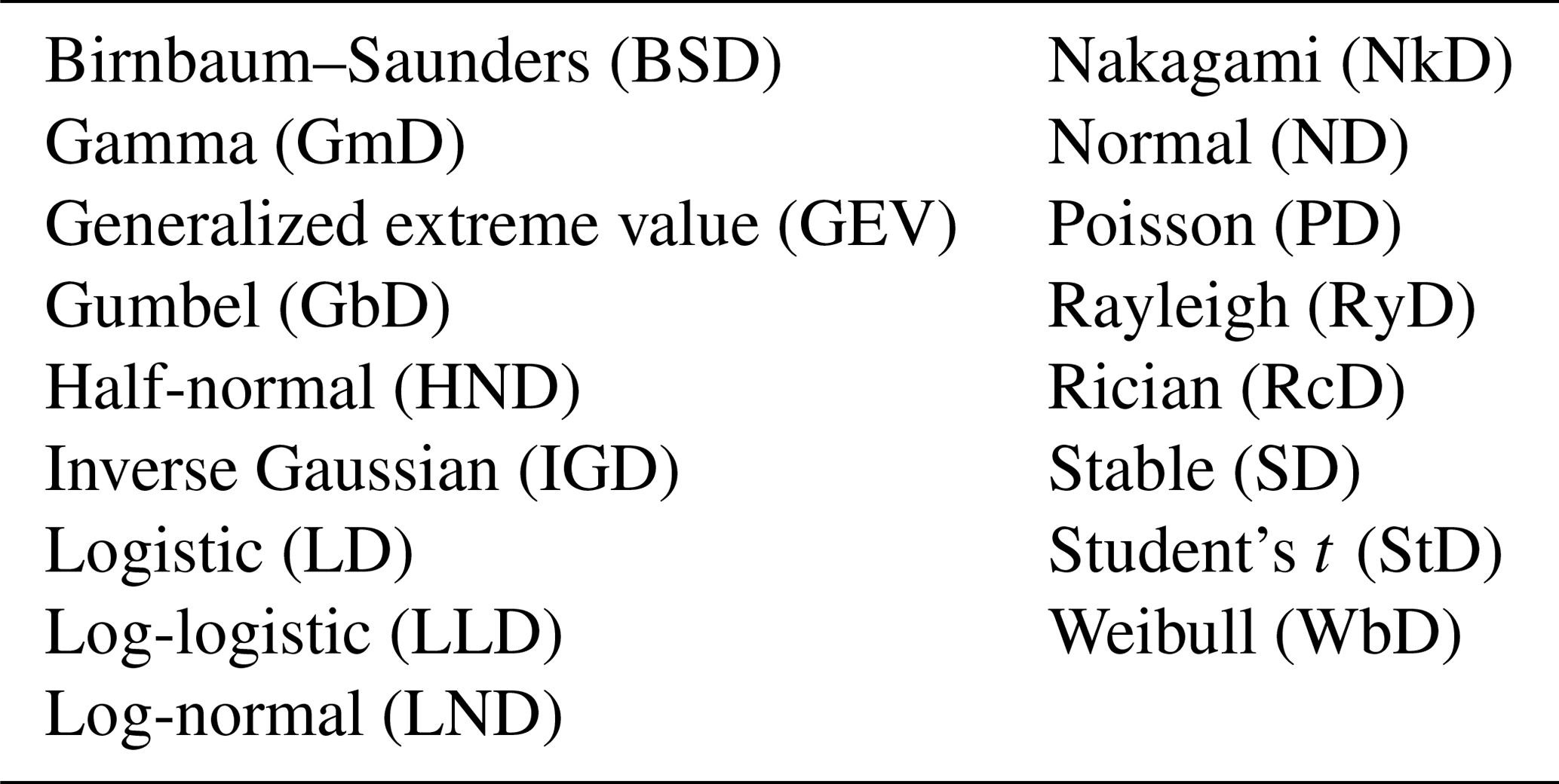
We used the 20 probability density functions (PDFs) preset in the MATLAB statistical toolbox (MATLAB, 2016) plus the circular von Mises distribution for wind speed (Mardia and Zemroch, 1975). In total, 17 PDFs were suitable and were tested and compared with the observed distribution of each parameter for each of the four seasons (Table A1). Note that the Gumbel distribution (GbD) and Weibull distribution (WbD) are special cases of the generalized extreme value distribution (GEV) and that some PDFs cannot be used due to their ranges.
Table A1List of the tested and suitable PDFs preset in the MATLAB statistical toolbox (the short acronyms in brackets are for further orientation).
A2 Skill score
In this study we use the skill score S introduced by Taylor (2001):
where r is the correlation coefficient after Spearman (1904) between the modeled and observed precipitation field, r0 is the maximum attainable correlation, and is the normalized standard deviation with the standard deviations of the model (SBM + M) σmod and observations (REGNIE) σobs. For and for r→r0, S approaches unity, which is the best result. Furthermore, Taylor (2001) provided no regulation for the estimation of r0. Therefore, we set r0 to the maximum calculated correlation coefficient of all simulations. As it is not guaranteed that this maximum is the actual maximum attainable correlation, we increase r0 by 10 %, yielding r0=0.93. According to Taylor (2001), the use of correlation and standard deviation is more stable compared to RMSE or bias.
A3 Return periods
For the estimation of return periods, the annual maximum series with length Tmax of the data set is sorted in descending order. Then, the return period Tk of each element xk of this series is given by with the rank rk(xk) of element xk. The first element (highest value) of the annual series, for example, of Tmax=100 years, has a return period of T1=100 years, the second has a return period of T2=50 years, and so on. For the visualization, the values of Tk were adjusted using the plotting position method of Cunnane (1978).
The supplement related to this article is available online at: https://doi.org/10.5194/hess-23-1083-2019-supplement.
MK designed the research. FE performed the research, the modellling, and the analysis. MK was involved in the interpretation of the results. FE mainly wrote the paper. MK extensively edited the paper and provided substantial comments and constructive suggestions for scientific clarification and further improvements.
The authors declare that they have no conflict of interest.
The authors thank a local insurance company for funding the project. We also
would like to thank the German Weather Service (DWD) and the Integrated
Global Radiosonde Archive (IGRA) for providing different observational data
sets and CGIAR-CSI for the orographic data. Special thanks go to James Daniell,
Andreas Kron. and Simon Hoellering from the Karlsruhe Institute of
Technology (KIT) for constructive discussions during the project and for
valuable suggestions for the model development. We acknowledge support by
the Deutsche Forschungsgemeinschaft (DFG) and open-access publishing fund of KIT.
We are grateful to the constructive and very helpful comments and suggestions
of the reviewers that helped to improve the scientific quality of this paper.
The article processing charges for this open-access
publication
were covered by a Research
Centre of the Helmholtz Association.
Edited by: Jan Seibert
Reviewed by: Nadav Peleg and three anonymous referees
Barstad, I. and Caroletti, G. N.: Orographic precipitation across an island in southern Norway: model evaluation of time-step precipitation, Q. J. Roy. Meteorol. Soc., 139, 1555–1565, 2013. a
Barstad, I. and Smith, R. B.: Evaluation of an Orographic Precipitation Model, J. Hydrometeorol., 6, 85–99, 2005. a, b, c, d, e, f, g
Basist, A., Bell, G. D., and Meentmeyer, V.: Statistical relationships between topography and precipitation patterns, J. Climate, 7, 1305–1315, 1994. a
Benoit, L., Allard, D., and Mariethoz, G.: Stochastic Rainfall Modeling at Sub-kilometer Scale, Water Resour. Res., 54, 4108–4130, https://doi.org/10.1029/2018WR022817, 2018. a, b
Bergeron, T.: On the physics of fronts, B. Am. Meteorol. Soc., 18, 265–275, 1937. a
Browning, K. A., Pardoe, C. W., and Hill, F. F.: The nature of orographic rain at wintertime cold fronts, Q. J. Roy. Meteorol. Soc., 101, 333–352, 1975. a
Cannon, D. J., Kirshbaum, D. J., and Gray, S. L.: Under what conditions does embedded convection enhance orographic precipitation?, Q. J. Roy. Meteorol. Soc., 138, 391–406, 2012. a, b
Caroletti, G. N. and Barstad, I.: An assessment of future extreme precipitation in western Norway using a linear model, Hydrol. Earth Syst. Sci., 14, 2329–2341, https://doi.org/10.5194/hess-14-2329-2010, 2010. a, b
Crochet, P., Jóhannesson, T., Jónsson, T., Sigurdsson, O., Björnsson, H., Pálsson, F., and Barstad, I.: Estimating the spatial distribution of precipitation in Iceland using a linear model of orographic precipitation, J. Hydrometeorol., 8, 1285–1306, 2007. a
Cross, D., Onof, C., Winter, H., and Bernardara, P.: Censored rainfall modelling for estimation of fine-scale extremes, Hydrol. Earth Syst. Sci., 22, 727–756, https://doi.org/10.5194/hess-22-727-2018, 2018. a
Cunnane, C.: Unbiased plotting positions – a review, J. Hydrol., 37, 205–222, 1978. a
Drogue, G., Humbert, J., Deraisme, J., Mahr, N., and Freslon, N.: A statistical-topographic model using an omnidirectional parameterization of the relief for mapping orographic rainfall, Int. J. Climatol., 22, 599–613, https://doi.org/10.1002/joc.671, 2002. a
Duckstein, L., Bárdossy, A., and Bogárdi, I.: Linkage between the occurrence of daily atmospheric circulation patterns and floods: an Arizona case study, J. Hydrol., 143, 413–428, 1993. a
Durran, D. R. and Klemp, J. B.: On the effects of moisture on the Brunt–Väisälä frequency, J. Atmos. Sci., 39, 2152–2158, 1982. a
Durre, I., Vose, R. S., and Wuertz, D. B.: Overview of the integrated global radiosonde archive, J. Climate, 1151, 53–68, 2006. a, b
Eliassen, A.: On the vertical circulation in frontal zones, Geophys. Publ., 24, 147–160, 1962. a
Fluck, E.: Hail statistics for European countries, PhD thesis, Institute of Meteorology and Climate Research (IMK), Karlsruhe Institute of Technologie (KIT), Karlsruhe, Germany, https://doi.org/10.5445/IR/1000080663, 2018. a
Freedman, D. and Diaconis, P.: On the histogram as a density estimator: L2 theory, Zeitschrift für Wahrscheinlichkeitstheorie und Verwandte Gebiete, 57, 453–476, https://doi.org/10.1007/BF01025868, 1981. a
Fuhrer, O. and Schär, C.: Embedded cellular convection in moist flow past topography, J. Atmos. Sci., 62, 2810–2828, 2005. a, b
Furrer, E. M. and Katz, R. W.: Generalized linear modeling approach to stoachstic weather generators, Clim. Res., 34, 129–144, 2007. a
Goovaerts, P.: Geostatistical approaches for incorporating elevation into the spatial interpolation of rainfall, J. Hydrol., 228, 113–129, 2000. a
Handwerker, J.: Cell tracking with TRACE3D – a new algorithm, Atmos. Res., 61, 15–34, 2002. a
Houze, R. A. and Hobbs, P. V.: Organization and Structure of Precipitation cloud systems, Adv. Geophys., 24, 225–315, 1982. a
Jiang, Q. and Smith, R. B.: Cloud timescales and orographic precipitation, J. Atmos. Sci., 60, 1543–1559, 2003. a, b
Kållberg, P., Simmons, A., Uppala, S., and Fuentes, M.: The ERA-40 archive, Shinfield Park, Reading, 2004. a
Kienzler, S., Pech, I., Kreibich, H., Müller, M., and Thieken, A. H.: After the extreme flood in 2002: changes in preparedness, response and recovery of flood-affected residents in Germany between 2005 and 2011, Nat. Hazards Earth Syst. Sci., 15, 505–526, https://doi.org/10.5194/nhess-15-505-2015, 2015. a
Kirshbaum, D. J. and Durran, D. R.: Factors governing cellular convection in orographic precipitation, J. Atmos. Sci., 61, 682–698, 2004. a
Kirshbaum, D. J. and Smith, R. B.: Temperature and moist-stability effects on midlatitude orographic precipitation, Q. J. Roy. Meteorol. Soc., 134, 1183–1199, https://doi.org/10.1002/qj.274, 2008. a, b
Koutsoyiannis, D., Kozonis, D., and Manetas, A.: A mathematical framework for studying rainfall intensity-duration-frequency relationships, J. Hydrol., 206, 118–135, 1998. a
Kunz, M.: Characterisitics of Large-Scale Orographic Precipitation in a Linear Perspective, J. Hydrometeorol., 12, 27–44, 2011. a, b, c, d, e, f, g, h, i, j, k, l, m
Kunz, M. and Wassermann, S.: Moist dynamics and sensitivity of orographic precipitation to changing ambient conditions in an idealised perspective, Meteorol. Z., 20, 199–215, 2011. a, b
Lalas, D. P. and Einaudi, F.: On the stability of a moist atmosphere in the presence of a background wind, J. Atmos. Sci., 30, 795–800, 1973. a
Maity, R.: Statistical Methods in Hydrology and Hydroclimatology, Springer Nature Singapore Pte Ltd., Singapore, https://doi.org/10.1007/978-981-10-8779-0, 2018. a
Mardia, K. V. and Zemroch, P. J.: Algorithm AS 86: The Von Mises Distribution Function, J. Roy. Stat. Soc. Ser. C, 24, 268–272, 1975. a, b
Marra, F., Morin, E., Peleg, N., Mei, Y., and Anagnostou, E. N.: Intensity–duration–frequency curves from remote sensing rainfall estimates: comparing satellite and weather radar over the eastern Mediterranean, Hydrol. Earth Syst. Sci., 21, 2389–2404, https://doi.org/10.5194/hess-21-2389-2017, 2017. a
MATLAB: MATLAB and Statistics Toolbox Release 2016b, (version 9.1), The MathWork Inc., Natick, Massachusetts, USA, available at: http://de.mathworks.com/help/ (last access: 10 August 2017), 2016. a, b
Mohr, S. and Kunz, M.: Recent trends and variabilities of convective parameters relevant for hail events in Germany and Europe, Atmos. Res., 123, 211–228, 2013. a
MunichRe: NatCatSERVICE, available at: https://natcatservice.munichre.com/, last access: 28 September 2017. a, b
Neykov, N. M., Neytchev, P. N., and Zucchini, W.: Stochstic daily precipitation model with a heavy-tailed component, Nat. Hazards Earth Syst. Sci., 14, 2321–2335, https://doi.org/10.5194/nhess-14-2321-2014, 2014. a
Palutikov, J. P., Brabson, B., Lister, D. H., and Adcock, S. T.: A review of methods to calculate extreme wind speeds, Meteorol. Appl., 6, 119–132, 1999. a
Paschalis, A., Molnar, P., Fatichi, S., and Burlando, P.: A stochastic model for high-resolution space-time precipitation simulation, Water Resour. Res., 49, 8400–8417, https://doi.org/10.1002/2013WR014437, 2013. a
Peleg, N., Fatichi, S., Paschalis, A., Molnar, P., and Burlando, P.: An advanced stochastic weather generator for simulating 2-D high-resolution climate variables, J. Adv. Model. Earth Syst., 9, 1595–1627, https://doi.org/10.1002/2016MS000854, 2017. a, b
Peleg, N., Marra, F., Fatichi, S., Paschalis, A., Molnar, P., and Burlando, P.: Spatial variability of extreme rainfall at radar subpixel scale, J. Hydrol., 556, 922–933, https://doi.org/10.1016/j.jhydrol.2016.05.033, 2018. a
Petrow, T., Zimmer, J., and Merz, B.: Changes in the flood hazard in Germany through changing frequency and persistence of circulation patterns, Nat. Hazards Earth Syst. Sci., 9, 1409–1423, https://doi.org/10.5194/nhess-9-1409-2009, 2009. a
Piper, D., Kunz, M., Ehmele, F., Mohr, S., Mühr, B., Kron, A., and Daniell, J.: Exceptional sequence of severe thunderstorms and related flash floods in May and June 2016 in Germany – Part 1: Meteorological background, Nat. Hazards Earth Syst. Sci., 16, 2835–2850, https://doi.org/10.5194/nhess-16-2835-2016, 2016. a
Rauthe, M., Steiner, H., Riediger, U. A. M., and Gratzki, A.: A Central European precipitation climatology – Part I: Generation and validation of a high-resolution gridded daily data set (HYRAS), Meteorol. Z., 22, 235–256, 2013. a, b
Reuter, H. I., Nelson, A., and Jarvis, A.: An evaluation of void-filling interpolation methods for SRTM data, Int. J. Geogr. Inf. Sci., 21, 983–1008, https://doi.org/10.1080/13658810601169899, 2007. a
Richardson, C. W.: Stochastic Simulation of Daily Precipitation, Temperature, and Solar Radiation, Water Resour. Res., 17, 182–190, 1981. a
Rockel, B., Will, A., and Hense, A.: The regional climate model COSMO-CLM (CCLM), Meteorol. Z., 17, 347–348, 2008. a
Schröter, K., Kunz, M., Elmer, F., Mühr, B., and Merz, B.: What made the June 2013 flood in Germany an exceptional event? A hydro-meteorological evaluation, Hydrol. Earth Syst. Sci., 19, 309–327, https://doi.org/10.5194/hess-19-309-2015, 2015. a, b, c
Singer, M. B., Michaelides, K., and Hobley, D. E. J.: STORM 1.0: a simple, flexible, and parsimonious stochastic rainfall generator for simulating climate and climate change, Geosci. Model Dev., 11, 3713–3726, https://doi.org/10.5194/gmd-11-3713-2018, 2018. a, b
Smith, R. B.: Linear theory of stratified hydrostatic flow past an isolated mountain, Tellus, 32, 348–364, 1980. a, b
Smith, R. B.: Hydrostatic airflow over mountains, Adv. Geophys., 31, 1–41, 1989. a
Smith, R. B. and Barstad, I.: A Linear Theory of Orographic Precipitation, J. Atmos. Sci., 61, 1377–1391, 2004. a, b, c, d, e, f
Spearman, C.: The Proof and Measurement of Association between Two Things, Am. J. Psychol., 15, 72–101, 1904. a, b, c, d
Taylor, K. E.: Summarizing multiple aspects of model performance in a single diagram, J. Geophys. Res., 106, 7183–7192, 2001. a, b, c, d
Uhlemann, S., Thieken, A. H., and Merz, B.: A consistent set of trans-basin floods in Germany between 1952–2002, Hydrol. Earth Syst. Sci., 14, 1277–1295, https://doi.org/10.5194/hess-14-1277-2010, 2010. a, b
Wanner, H., Rickli, R., Salvisberg, E., Schmutz, C., and Schüepp, M.: Global climate change and variability and its influence on alpine climate-concepts and observations, Theor. Appl. Climatol., 58, 221–243, 1997. a
Wilks, D. S.: Statistical Methods in the Atmospheric Sciences, in: vol. 91 of International Geophysics Series, 2nd Edn., Academie Press, San Diego, California, USA, 2006. a
- Abstract
- Introduction
- Stochastic precipitation model
- Data sets
- Calibration
- Parameter estimation of the stochastic simulations
- Stochastic event set and model validation
- Summary and conclusions
- Data availability
- Appendix A: Statistical quantities
- Author contributions
- Competing interests
- Acknowledgements
- References
- Supplement