A simple model for local-scale sensible and latent heat advection contributions to snowmelt

Local-scale advection of energy from warm snow-free surfaces to cold snow-covered surfaces is an important component of the energy balance during snow-cover depletion. Unfortunately, this process is difficult to quantify in one-dimensional snowmelt models. This paper proposes a simple sensible and latent heat advection model for snowmelt situations that can be readily coupled to one-dimensional energy balance snowmelt models. An existing advection parameterization was coupled to a conceptual frozen soil infiltration surface water retention model to estimate the areal average sensible and latent heat advection contributions to snowmelt. The proposed model compared well with observations of latent and sensible heat advection, providing confidence in the process parameterizations and the assumptions applied. Snow-covered area observations from unmanned aerial vehicle imagery were used to update and evaluate the scaling properties of snow patch area distribution and lengths. Model dynamics and snowmelt implications were explored within an idealized modelling experiment, by coupling to a one-dimensional energy balance snowmelt model. Dry, snow-free surfaces were associated with advection of dry air that compensated for positive sensible heat advection fluxes and so limited the net influence of advection on snowmelt. Latent and sensible heat advection fluxes both contributed positive fluxes to snow when snow-free surfaces were wet and enhanced net advection contributions to snowmelt. The increased net advection fluxes from wet surfaces typically develop towards the end of snowmelt and offset decreases in the one-dimensional areal average melt energy that declines with snow-covered area. The new model can be readily incorporated into existing one-dimensional snowmelt hydrology and land surface scheme models and will foster improvements in snowmelt understanding and predictions.

1 Introduction

Sensible and latent turbulent heat fluxes contributing to snowmelt are complicated during snow-covered area (SCA) depletion by the lateral redistribution of energy from snow-free surfaces to snow. Unfortunately, many calculations of the snow surface energy balance have largely been limited to one-dimensional model frameworks (Brun et al., 1989; Gray and Landine, 1988; Jordan, 1991; Lehning et al., 1999; Marks et al., 1999) which simulate melt at points without considering variations in SCA. Despite the sophistication of these methods, they have neglected local-scale advection of energy.

The differences in surface energetics between snow-covered and snow-free areas lead to a heterogeneous distribution of surface temperature and near-surface water vapour. These horizontal gradients drive a lateral exchange of heat (sensible heat advection) and water vapour (latent heat advection when considering the induced condensation or sublimation) over the leading edge of a snow patch. Advection contributions to snowmelt are not negligible as sensible heat advection has been estimated to account for up to 55 % of the snowmelt energy balance (Granger and Male, 1978), resulting in areal melt rates being greatest when snow cover is between 40 % and 60 % (Shook, 1995; Marsh et al., 1997). Advection is very challenging to directly observe due to the dynamic nature of snow-cover ablation. Direct observations of the melt implications of advection have utilized repeat terrestrial laser scanning to identify and quantify larger melt rates on the leading edge of snow patches (Mott et al., 2011). The development of internal boundary layers as air flows over heterogenous surfaces provides an alternate approach to measure the advection energy flux directly (Garratt, 1990). Measurements of these internal boundary layers across snow surface transitions reflect established power laws of boundary layer height (Shook, 1995; Granger et al., 2006) and can quantify the latent and sensible heat advection through boundary layer integration (Granger et al., 2002, 2006; Harder et al., 2017). In contrast to these findings the formation of boundary layers has also been identified as a potential cause of atmospheric decoupling of the atmosphere from the snow surface, leading to the suppression of sensible heat advection in the Alps (Mott et al., 2013, 2016, 2017). The reader is referred to Fujita et al. (2010), Granger et al.(2002, 2006), Mott et al. (2013, 2016, 2017) and Sauter and Galos (2016) for discussions on the complexities of boundary layer development over snow during advection situations and how this may influence overall energy exchange. Due to the complexity of the process and difficulties in observation, modelling has been the focus of much more work on this topic.

To model advection to snow patches, Weisman (1977) applied mixing length theory, implicitly accounting for both latent heat advection (LE_A) and sensible heat advection (H_A). This work was proposed at a time when knowledge of the statistical properties of snow cover were inadequate for easy extension to natural snowpacks. Gray et al. (1986) noted that

The major obstacle to the development of an energy balance model for calculating melt quantities is the lack of reliable methods for evaluating the sensible heat flux. A priority research need is the development of “bulk methodologies” for calculating this term, especially for patchy, snow-cover conditions.

Subsequent models have had variable complexity. Marsh and Pomeroy (1996) estimated areal average H_A via a simple advection efficiency term related to SCA. Another approach to estimate areal average estimates of advection applied internal boundary layer integration approaches (Granger et al., 2002, 2006) to tile models (Essery et al., 2006) and accounted for the scaling properties of natural snow cover (Shook et al., 1993a). Other investigations have employed complex atmospheric boundary layer models (Liston, 1995) and large eddy simulation (Mott et al., 2015, 2017; Sauter and Galos, 2016) to quantify the non-linear relationships between snow patch characteristics/geometry and advected energy. Numerical models provide the most detailed description of the processes but are constrained to idealized boundary conditions. The problem with all these modelling approaches is that none have had validation with actual advection observations and LE_A has largely been ignored. Only Liston (1995) considered LE_A, but in that study did not explicitly partition advected energy into H_A or LE_A components and assumed a constant saturated snow-free surface. This is in contrast to observations of LE_A that show a dependency upon the dynamic extent of ponded meltwater (and associated dynamic near-surface humidity content) which is prevalent in areas of low topographic relief and limited snowmelt infiltration due to frozen soils (Harder et al., 2017). The main challenges in modelling these dynamics is to constrain the areal extent over which the advection exchange takes place, quantify the gradients in scalar between upwind and downwind surfaces, and relate the scalar gradients to advection fluxes.

There remains a pressing need for an approach that can estimate areal average H_A and LE_A contributions during snowmelt that can easily integrate with existing one-dimensional snowmelt models. This work seeks to understand the implications of including local-scale H_A and LE_A with one-dimensional snowmelt models. To address this objective, this paper presents a simple and easily implementable H_A and LE_A model. The specific objectives are to validate the proposed model with observations of advection, to re-evaluate the scaling relationships of snow-cover geometry with current datasets of snow cover and to quantify the implications of including advection upon snowmelt.

2 Methodology

The methodology to address the research objectives is briefly outlined here. A conceptual and quantitative model framework extended the Granger et al. (2002) advection model, hereafter referred to as the extended GM2002, to also consider LE_A. The performance of the extended GM2002 was evaluated with respect to H_A and LE_A observations as reported in Harder et al. (2017). Snow-cover geometry scaling relationships employed in the model framework (Granger et al., 2002; Shook et al., 1993b), originally based on SCA classifications from coarse-resolution or oblique imagery, were re-evaluated with high-resolution unmanned aerial vehicle (UAV) imagery. The complete model framework, hereafter referred to as the Sensible and Latent Heat Advection Model (SLHAM), was then used to explore the dynamics of the extended GM2002 when coupled with parameterizations for frozen soil infiltration and the relationship between surface detention storage and fractional water area. Snowmelt simulation performance and the implications of including H_A and LE_A were explored by coupling SLHAM to the Stubble–Snow–Atmosphere snowmelt Model (SSAM) (Harder et al., 2018). The SSAM accounts for the dynamic influence of crop stubble emergence on the sensible and latent heat and shortwave and longwave radiation terms of the snow surface energy balance that is coupled to the mass balance of a single-layer snowpack model to simulate snowmelt. Development and validation for SSAM focused on representing snowmelt of shallow snowpacks in the agricultural regions of the Canadian Prairies. SLHAM is coupled to SSAM here as a demonstration of its ability to be coupled to existing snowmelt energy balance models that assume continuous snow cover. Other snowmelt models could similarly be easily coupled to SLHAM. The model performance of SSAM and SSAM–SLHAM was also compared against the Energy Balance Snowmelt Model (EBSM; Gray and Landine, 1988), a snowmelt model commonly implemented for snowmelt prediction on the Canadian Prairies. In EBSM the contribution of advection energy is indirectly addressed through simulation of an areal average albedo that varies from a maximum of 0.8 pre-melt, a continuous snow surface, to approach a low of 0.2 at the end of melt, which represents bare soil rather than old snow (Gray and Landine, 1987). The areal average net radiation, greater than typically received by a continuous snow surface, is assumed to contribute to areal average snowmelt, thereby implicitly accounting for advection. While a simple approach to include advection energy for snowmelt, it is unconstrained by SCA dynamics and will overestimate melt for low values of SCA. The implications of including advection were evaluated with initial conditions and driving meteorology observed over two snowmelt seasons from a research site located in the Canadian Prairies.

2.1 Model framework

Horizontal gradients of scalar properties are a first-order control on the advection flux. For snowmelt the gradients are conceptualized as snow-free surfaces upwind of a transition to a snow-covered surface. During melt periods upwind snow-free surfaces are typically comprised of dry soil and/or ponded water which correspond to warm dry and/or warm moist near-surface air properties, respectively. In contrast snow is commonly assumed to be ≤0 ^∘C with saturated near-surface air (Fig. 1a). Conceptual air temperature and specific humidity profiles over snow, soil, and water surfaces are shown in Fig. 1b to articulate the atmospheric boundary layer dynamics observed by Granger et al. (2002, 2006) and Harder et al. (2017). Assuming the changes in profiles are solely due to exchange with the surface the magnitude and direction of the energy flux can be quantified by the integrated differences in profiles between the surface and the mixing height; the point above the surface where differences due to surface heterogeneity disappear with atmospheric mixing (Granger et al., 2002). When the upwind snow-free surface is warm the cooling of the air as it moves over the snow will lead to sensible heat advection to the snowpack and vice versa. Latent heat advection is dependent upon surface temperature as well as saturation. Thus, air from a dry soil may increase in humidity as it moves over snow, which induces greater sublimation and therefore a reduction in snowmelt energy (Harder et al., 2017). In contrast, a wet upwind condition will lead to a decrease in humidity as the air moves over the relatively drier snow due to condensation upon the snow surface, which imparts a release of latent heat or an increase in snowmelt energy (Harder et al., 2017).

Figure 1 (a) Conceptual cross section of the advection process during snowmelt and (b) conceptual specific humidity and air temperature profiles between snow (0 ^∘C, 100 % RH), soil (6 ^∘C, 60 % RH) and water (1 ^∘C, 100 % RH) surfaces and the mixing height (3 ^∘C, RH of 60 %).

To scale any estimate of fetch length advection to an areal average representation the geometric properties and extent of exchange are needed. Over the course of melt, SCA declines from completely snow-covered to snow-free conditions, with the intermediate periods defined by a heterogeneous blend of both. Conceptually the advection of energy to snow therefore is bounded by the areas of snow-free and snow-covered surfaces that constrain energy transfer. Initial advection contributions to melt are dominated by energy advecting from emerging snow-free patches to the surrounding snow (Fig. 2a). The total amount of energy advected will be limited by the smaller snow-free surface source area available to exchange energy; all energy entrained by air movement across isolated snow-free patches will be completely advected to the surrounding snow surfaces. At the end of snowmelt, snow patches remain in a snow-free domain, and some energy is advected from the warm surrounding snow-free surface to isolated snow patches (Fig. 2b). The amount of energy advected is limited by the smaller snow surface area available to exchange energy. When the snow surface is the most heterogeneous, with a complex mixture of snow and snow-free patches, advection occurs between isolated snow-free patches, surrounding snow cover, snow-free surfaces, and isolated snow patches at the same time. Conceptually there will be a gradual transition from isolated snow-free patch to isolated snow patch advection constraints. Marsh and Pomeroy (1996) and Shook et al. (1993b) found that magnitude of the snowmelt advection flux will be greatest when SCA is 40 %–60 % and this range was used to bound the transition of advection constraints. The advection mechanism transitions over the course of the melt and was conceptually related to SCA by a fractional source (f_s) term that assumes a linear weighting between 60 % and 40 % SCA as

$$\begin{array}{}\text{(1)}& f_{\mathrm{s}}=\begin{array}{ll}\mathrm{1}& \mathrm{SCA}>\mathrm{0.6},\\ \left({\displaystyle \frac{\mathrm{SCA}-\mathrm{0.4}}{\mathrm{0.2}}}\right)& \mathrm{0.4}\le \mathrm{SCA}\le \mathrm{0.6},\\ \mathrm{0}& \mathrm{SCA}<\mathrm{0.4}.\end{array}\end{array}$$

An f_s of 1 implies the exchange of advection energy is limited by the snow-free patch areas and an f_s of 0 implies the exchange of advection energy is limited by the snow patch areas. Conceptually early advection from snow-free patches will have a more effective energy exchange mechanism than later advection to isolated snow patches. The unstable temperature profile above a relatively rough warm snow-free surface patch will enhance exchange with the atmosphere, and therefore surrounding snow cover, per unit area of snow-free surface. In contrast, the stable temperature profiles above a cool and smooth isolated snow patch will limit energy exchange per unit area of snow surface. The stability influences upon surface exchange dynamics are implicitly accounted for in the parameterization of stability terms by Weisman (1977) and are expressed in Sect. 2.1.1.

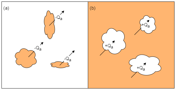
Figure 2 Conceptual model of advection dynamics for (a) the early melt period where energy is limited to what is transported out of soil (brown) patches to the surrounding snow (white), and for (b) the later melt period where snow patches remain and advection energy is limited to that exchanged over the discrete patches.

During snowmelt, meltwater may infiltrate into the frozen soil and any excess will pond prior to and during the runoff phase; these interactions will influence the near-surface humidity of the snow-free surface. Thus, LE_A may enhance sublimation when the upwind surface is dry or condense and enhance melt when the upwind surface is wet (Harder et al., 2017). Any attempt to model advection must quantify the dynamic spatial properties of the snow and snow-free patch distributions, SCA, fractional water coverage of ponded water, and horizontal gradients of temperature and humidity between snow and snow-free surfaces. With quantification of these processes, existing simple advection parametrizations can be extended to calculate H_A and LE_A contributions to snowmelt in a manner that accounts for the dynamics of the driving variables and processes and still be easily implemented in snowmelt energy balance models. The SLHAM model quantifies the components of the conceptual model outlined in Figs. 1 and 2.

Table 1 Parameterizations for extended GM2002.

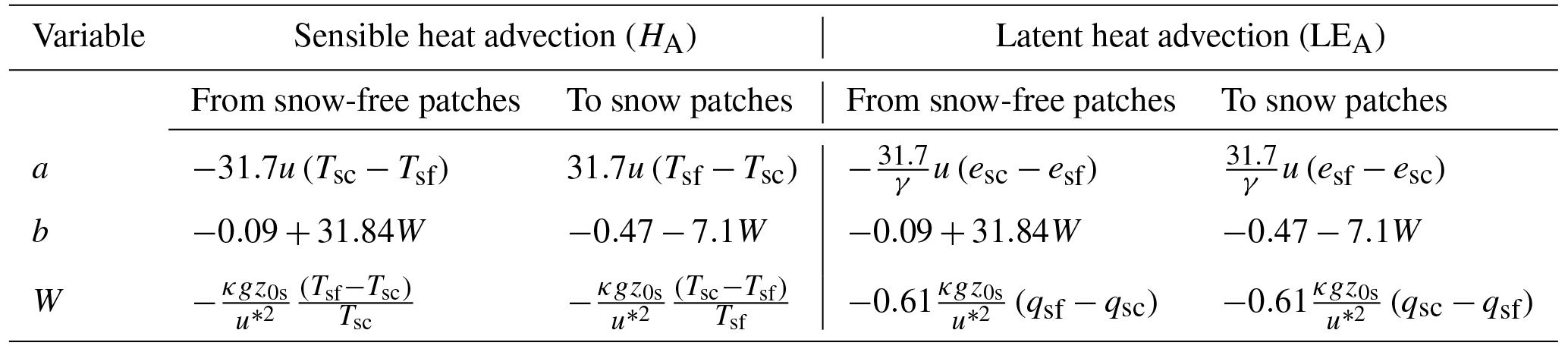
e_sc: snow surface vapour pressure (kPa); T_sc: snow surface temperature (K); e_sf: snow-free surface vapour pressure (kPa); T_sf: snow-free surface temperature(K); g: acceleration due to gravity (9.81 m s⁻²); u: wind speed (m s⁻¹); κ: von Kármán constant (0.4); u^∗: friction velocity (m s⁻¹); q_sc: snow surface specific humidity (kg kg⁻¹); z_0s: snow surface roughness (0.005 m); q_sf: snow-free surface specific humidity (kg kg⁻¹); γ: psychrometric constant (kPa K⁻¹).

2.1.1 Advection versus distance from surface transition

Granger et al. (2002) developed a simplified approach to estimate the advection over a surface transition from boundary layer integration. Advected energy, Q_A (W m⁻²), was presented as a power function of patch length, L (m), downwind of a surface transition as

$$\begin{array}{}\text{(2)}& Q_{\mathrm{A}}\left(L\right)=a{L}^b.\end{array}$$

The coefficient a (W m⁻²) scales with wind speed and the horizontal scalar gradient and the coefficient b (–) is a function of the Weisman (1977) stability parameters (W). Parametrizations for these coefficients vary for sensible (H_A) and latent (LE_A) heat advection and whether advection is from a snow-free patch or to a snow patch; parametrizations are summarized in Table 1. The GM2002 approach is restricted to considering H_A contributions to snow. To extend this approach to LE_A the a and b parameterizations of GM2002 were assumed to remain valid. The parameterization for coefficient a in the case of LE_A was modified to use the surface vapour pressure gradient (kPa) with division by the psychrometric constant (γ, kPa K⁻¹). This relates the horizontal water vapour gradient to be in terms of an equivalent temperature gradient; in the units of the original a parametrization. The coefficient b for LE_A uses the humidity stability parameter of Weisman (1977) rather than the temperature stability parameter.

The humidity of the air at the surface interface is rarely observed but is needed to quantify the LE_A term. The e_sc was estimated by assuming saturation at the T_sc. The e_sf is more challenging as it varies with the surface fraction of ponded water (F_water, no unit) as

$$\begin{array}{}\text{(3)}& e_{\mathrm{sf}}=F_{\mathrm{water}}{e}_{\mathrm{wat}}+\left(\mathrm{1}-F_{\mathrm{water}}\right)e_{\mathrm{soil}}.\end{array}$$

The surface water vapour pressure for water surfaces (e_wat, kPa) was estimated by assuming saturation at the surface temperature of the ponded water (T_wat, K). Assuming negligible evaporation from dry soil surfaces during snowmelt, the surface water vapour of soil (e_soil, kPa) can be taken to be the same as actual vapour pressure observed above the surface. The T_sf was also weighted by F_water as

$$\begin{array}{}\text{(4)}& T_{\mathrm{sf}}=F_{\mathrm{water}}{T}_{\mathrm{wat}}+\left(\mathrm{1}-F_{\mathrm{water}}\right)T_{\mathrm{soil}},\end{array}$$

where T_soil (K) is the dry soil surface temperature. The remaining uncertainties in applying this framework are the representation of the statistical distribution of L, and estimation of F_water and SCA.

2.1.2 Fractional coverage of ponded water

To estimate F_water, the meltwater in excess of frozen soil infiltration capacity was estimated using the parametric frozen soil infiltration equation of Gray et al. (2001). Gray et al. (2001) parameterized the maximum infiltration of the limited condition (INF, mm) as

$$\begin{array}{}\text{(5)}& \mathrm{INF}=C{S}_{\mathrm{0}}^{\mathrm{2.92}}{\left(\mathrm{1}-S_i\right)}^{\mathrm{1.64}}{\left({\displaystyle \frac{\mathrm{273.15}-T_{\mathrm{si}}}{\mathrm{273.15}}}\right)}^{-\mathrm{0.45}}{t}_{\mathrm{0}}^{\mathrm{0.44}},\end{array}$$

where C (2.1, no unit) is a coefficient representing prairie soils, S₀ (–) is a surface saturation (generally assumed to be 1), S_i (–) is the antecedent soil saturation, T_si (K) is the initial soil temperature, and t₀ (h) is the infiltration opportunity time. The t₀ term is estimated as the cumulative hours of active snowmelt over the course of the snowmelt period. Excess meltwater (M_excess, mm) is calculated as

$$\begin{array}{}\text{(6)}& M_{\mathrm{excess}}=\sum _{t=\mathrm{0}}^i{M}_t-{\mathrm{INF}}_i,\end{array}$$

where M (mm) is the snowmelt since the beginning of melt (t=0) to the present time step i.

To relate M_excess to F_water, an elevation profile of the microtopography must be known. For simplicity, the furrows that define the microtopography of an agricultural field were assumed to be represented by a half-period, trough to peak, of a sine curve (Fig. 3). Thus F_water is given by the solution of

$$\begin{array}{}\text{(7)}& S_{\mathrm{ret}}={\displaystyle \frac{\mathrm{1}}{\mathit{\pi }}}\sin \left(F_{\mathrm{water}}\mathit{\pi }\right)-F_{\mathrm{water}}\cos \left(F_{\mathrm{water}}\mathit{\pi }\right),\end{array}$$

where the ratio of filled detention storage (S_ret, no unit) is determined from

$$\begin{array}{}\text{(8)}& S_{\mathrm{ret}}={\displaystyle \frac{M_{\mathrm{excess}}}{S_{max}}},\end{array}$$

where a user-defined S_max (mm) is the maximum detention storage of the surface. Any M_excess that is greater than S_max is removed as runoff and thereafter unavailable to future infiltration.

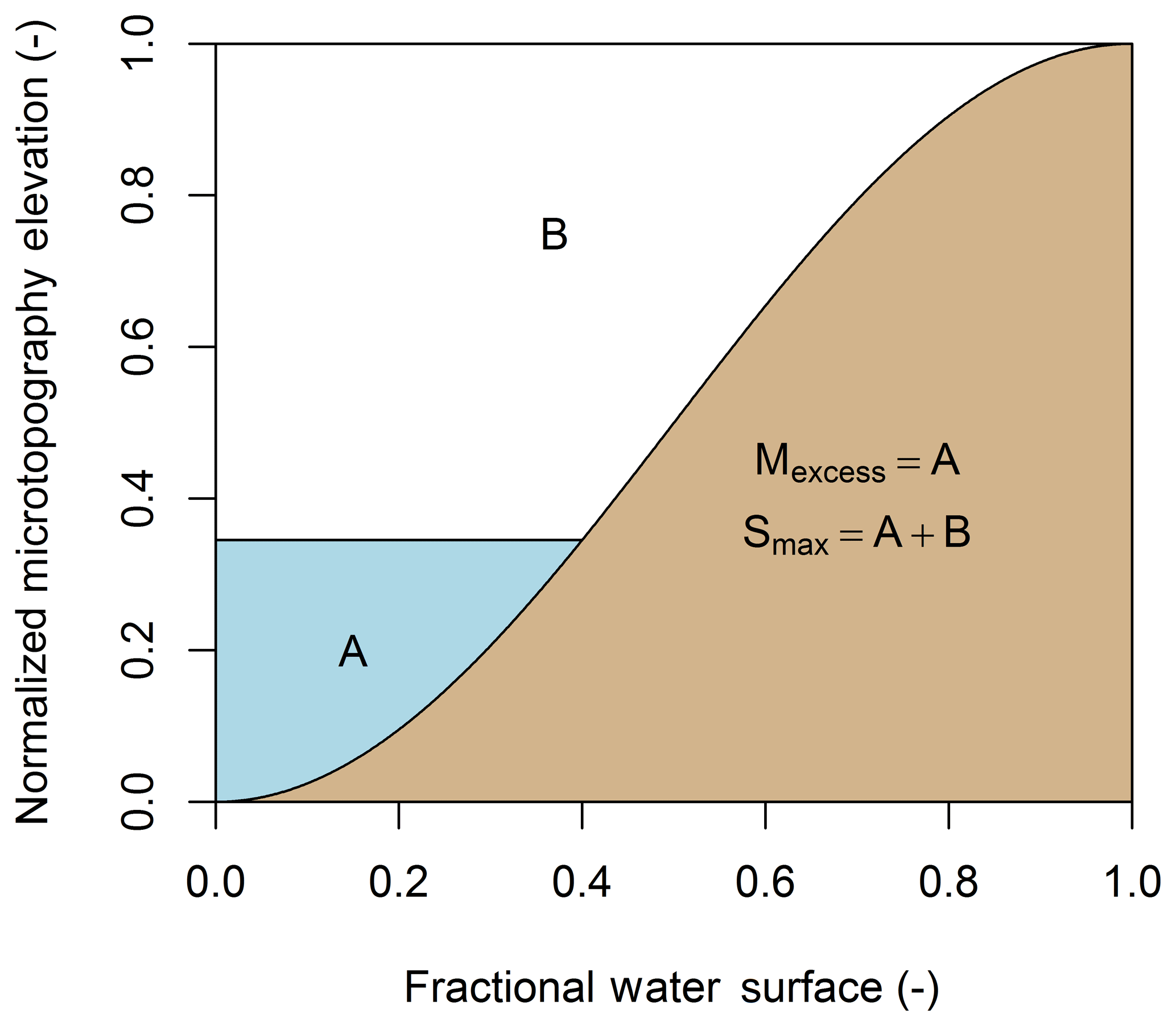
Figure 3 Conceptual water area–volume relationship diagram where a cross section of land surface microtopography (brown is soil and blue is water) is assumed to follow a sinusoidal profile.

2.1.3 Snow-covered area

The SCA constrains the overall exchange of energy between the snow surface and the atmosphere. Essery and Pomeroy (2004) developed an SCA parameterization from the closed form fit to the parametric SCA curve produced by homogeneous melt of a log-normal SWE distribution,

$$\begin{array}{}\text{(9)}& \mathrm{SCA}=\tanh \left(\mathrm{1.26}{\displaystyle \frac{\mathrm{SWE}}{{\mathit{\sigma }}_{\mathrm{0}}}}\right),\end{array}$$

where SWE is in mm and σ₀ (mm) is the standard deviation of SWE at the pre-melt maximum accumulation. The σ₀ constrains the spatial variability of a snowpack and how it relates to SCA depletion. Snow cover with high spatial variability will have a longer duration of patchiness and therefore advection will contribution to more of the total snowmelt. Other parameterizations of SCA exist and this was selected for its simplicity, relative success in describing observed SCA curves, and derivation in similar environments with regard to what is being modelled.

2.1.4 Snow geometry

Perimeter–area relationships and patch area distributions of snow and snow-free patches show fractal characteristics that can be exploited to simplify the representation of snow-cover geometry needed to calculate advection. There are two commonly used scaling relationships. From application of Korcak's law by Shook et al. (1993a) the fraction of snow patches greater than a given area, F(A_p), is given as a power law distribution

$$\begin{array}{}\text{(10)}& F\left(A_{\mathrm{p}}\right)={{\displaystyle \frac{A_{\mathrm{p}}}{c_{\mathrm{1}}}}}^{-D_k/\mathrm{2}},\end{array}$$

where c₁ is a threshold value (given as the smallest patch size observed, and hereafter taken as 1 m²), A_p (m²) is patch area, and D_k (–) is the scaling dimension. The scaling dimension is the same between snow and snow-free patches, relatively invariant with time, and ranges between 1.2 and 1.6 (Shook et al., 1993b) and is not a fractal dimension (Imre and Novotn, 2016). A Hack's law relationship between linear dimension and area of landscape features was established by Rigon et al. (1996) and this was extended to A_p and L of snow patches by Granger et al. (2002) as

$$\begin{array}{}\text{(11)}& L=c_{\mathrm{2}}\cdot A_{\mathrm{p}}^{\frac{D^{\prime }}{\mathrm{2}}},\end{array}$$

where c₂ is a constant taken as 1 and D^′ was fitted by Granger et al. (2002) to be 1.25.

The relationships of Eqs. (10) and (11) were exploited to develop a probability distribution of L. The exceedance fraction, Eq. (10), was converted to a probability distribution with calculation of probabilities for discrete intervals; this also entailed appropriate selection of intervals. The patch area probability (p(A_p)) is also equivalent to the probability associated with the probability of patch length (p(L)), therefore

$$\begin{array}{}\text{(12)}& p\left(L_i\right)=p\left(A_{{\mathrm{p}}_{\mathrm{i}}}\right)=F\left(A_{{\mathrm{p}}_{\mathrm{i}}-\mathrm{1}}\right)-F\left(A_{{\mathrm{p}}_{\mathrm{i}}}\right),\end{array}$$

where i is the index for intervals of A_p that span a range constrained as $c_{\mathrm{1}}\le A_{\mathrm{p}}<\mathrm{\infty }$. A discrete bin width of ≤1 m is advised to capture the large change in F(A_p) at the more frequent small values of A_p. To estimate an areal average advection exchange the normalized areal extent of each patch size was calculated. The limited number of the largest patches will dominate the exchange surface extent. Thus $p\left(A_{{\mathrm{p}}_{\mathrm{i}}}\right)$ is transformed to give a normalized areal fraction of the unit area that is represented by each patch size $f\left(A_{{\mathrm{p}}_{\mathrm{i}}}\right)$ as

$$\begin{array}{}\text{(13)}& f\left(A_{{\mathrm{p}}_{\mathrm{i}}}\right)={\displaystyle \frac{p\left(A_{{\mathrm{p}}_{\mathrm{i}}}\right)A_{{\mathrm{p}}_{\mathrm{i}}}}{\sum p\left(A_{{\mathrm{p}}_{\mathrm{i}}}\right)A_{{\mathrm{p}}_{\mathrm{i}}}}}.\end{array}$$

The transformation of the probability of occurrence to a fractional area of patch size is visualized in Fig. 4.

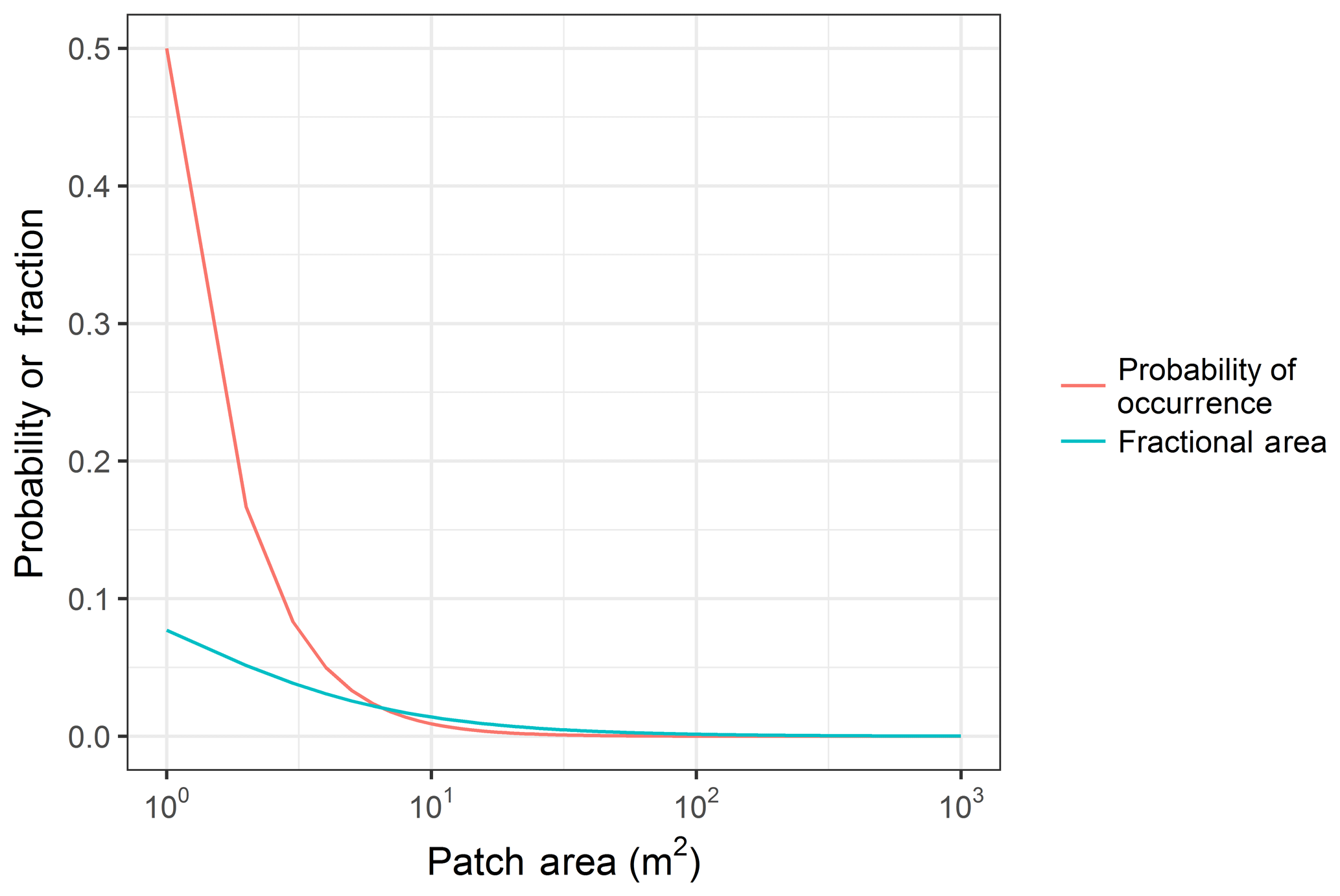
Figure 4 Probability of patch size occurrence and its transformation to fractional area patch sizes for a range in patch sizes from 1 to 1000 m².

2.1.5 Areal average advection

Using the above-described parameterizations of $f\left(A_{{\mathrm{p}}_{\mathrm{i}}}\right)$, L, SCA, F_water and INF, as well as boundary layer integration H_A and LE_A parameterizations, the areal average advection, $\stackrel{\mathrm{‾}}{Q_{\mathrm{A}}}$ (W), can be calculated as

$$\begin{array}{ll}{\displaystyle }\stackrel{\mathrm{‾}}{Q_{\mathrm{A}}}=& {\displaystyle }{f}_{\mathrm{s}}\left(\mathrm{1}-\mathrm{SCA}\right)\sum _{i=\mathrm{1}}^{i=A_{max}}f\left(A_{{\mathrm{p}}_{\mathrm{i}}}\right)H_{\mathrm{A},\mathrm{sf}}\\ {\displaystyle }& {\displaystyle }+\left(\mathrm{1}-f_{\mathrm{s}}\right)\mathrm{SCA}\sum _{i=\mathrm{1}}^{i=A_{max}}f\left(A_{{\mathrm{p}}_{\mathrm{i}}}\right)H_{\mathrm{A},\mathrm{sc}}\\ {\displaystyle }& {\displaystyle }+f_{\mathrm{s}}\left(\mathrm{1}-\mathrm{SCA}\right)\sum _{i=\mathrm{1}}^{i=A_{max}}f\left(A_{{\mathrm{p}}_{\mathrm{i}}}\right){\mathrm{LE}}_{\mathrm{A},\mathrm{sf}}\\ \text{(14)}& {\displaystyle }& {\displaystyle }+\left(\mathrm{1}-f_{\mathrm{s}}\right)\mathrm{SCA}\sum _{i=\mathrm{1}}^{i=A_{max}}f\left(A_{{\mathrm{p}}_{\mathrm{i}}}\right){\mathrm{LE}}_{\mathrm{A},\mathrm{sc}}.\end{array}$$

The terms from left to right represent the H_A from snow-free patches, H_A to snow patches, LE_A from snow-free patches, and LE_A to snow patches. All summation terms constitute H_A and LE_A for the range of patch areas expected, from 1 m² to an environment appropriate maximum expected patch size (A_max, m²). Calculation of H_A and LE_A use Eq. (2) with application of appropriate a and b parameterizations from Table 1 and L as calculated with Eq. (11) from the range of A_p. Advection fluxes for the range of patch sizes encountered are weighted by $f\left(A_{{\mathrm{p}}_{\mathrm{i}}}\right)$, Eq. (13), to give an areal average maximum flux. The advection process must be constrained to snow-free or snow surfaces over which exchange takes place, hence the scaling of the maximum advection by (1−SCA) and SCA from snow-free patches and to snow patches respectively. The f_s and (1−f_s) terms quantify the relative contribution from snow-free patches and to snow patches over snowmelt and SCA depletion. The primary controls on the model behaviour are the horizontal gradients of humidity and temperature, as well as wind speed.

2.2 Re-evaluation of snow-geometry scaling relationships

The coefficients for the snow-cover geometry relationships are based on oblique terrestrial photography or aerial photography with coarse resolution and limited temporal sampling (Shook et al., 1993b). Recent advances in UAV technologies provide a tool to re-evaluate these relationships with georectified high-resolution imagery. During the 2015 and 2016 snowmelt seasons, 0.035 m × 0.035 m spatial resolution red–green–blue (RGB) imagery was collected daily during active melt. This imagery was classified into snow and non-snow areas with pixel-based supervised thresholding of blue band reflectance. Cells that share the same classification and were connected via any of the four mutually adjacent cell boundaries were grouped into snow and non-snow patches. The SDMTools R package (VanDerWal et al., 2014) was used to calculate patch areas. Patch length is a challenging to define and quantify. For this analysis a similar approach to Granger et al. (2002) was used in which the patch length was calculated as the mean of the height and width of the minimum rotated bounding box that contained the entire snow patch. Patches with areas less than 1 m² were removed from the analysis as noise and classification artefacts are associated with such small patch sizes. The 1 m² area threshold is consistent with the existing literature on advection and snow-cover geometry (Granger et al., 2002; Shook et al., 1993b, a). When SCA was less than 50 %, snow patch metrics were quantified, and when SCA was greater than 50 %, snow-free patch metrics were quantified. An example is provided in Fig. 5.

2.3 Model dynamics

The influence of the advection model upon snowmelt dynamics was explored with two approaches. The first approach is a scenario and sensitivity analysis where inputs are fixed and a selection of process parameterizations are employed to illustrate the relationship between H_A and LE_A and the snow-free surface humidity dynamics and snowmelt implications. The second approach coupled the SLHAM with an existing one-dimensional snowmelt model to estimate the influence of including, or not including, the advection process on snowmelt simulations.

Figure 5 Example of snow-cover geometry scaling properties, exceedance faction versus patch area (b, D_k=21) and patch length versus patch area (c, $D^{\prime }=\mathrm{122}$), for snow-covered area classification at 1 m resolution from 29 March 2016 (a, axes are UTM 13N northing and eastings). Red lines are the best-fit scaling relationships, where slope provides the scaling constant.

2.3.1 Scenario analysis

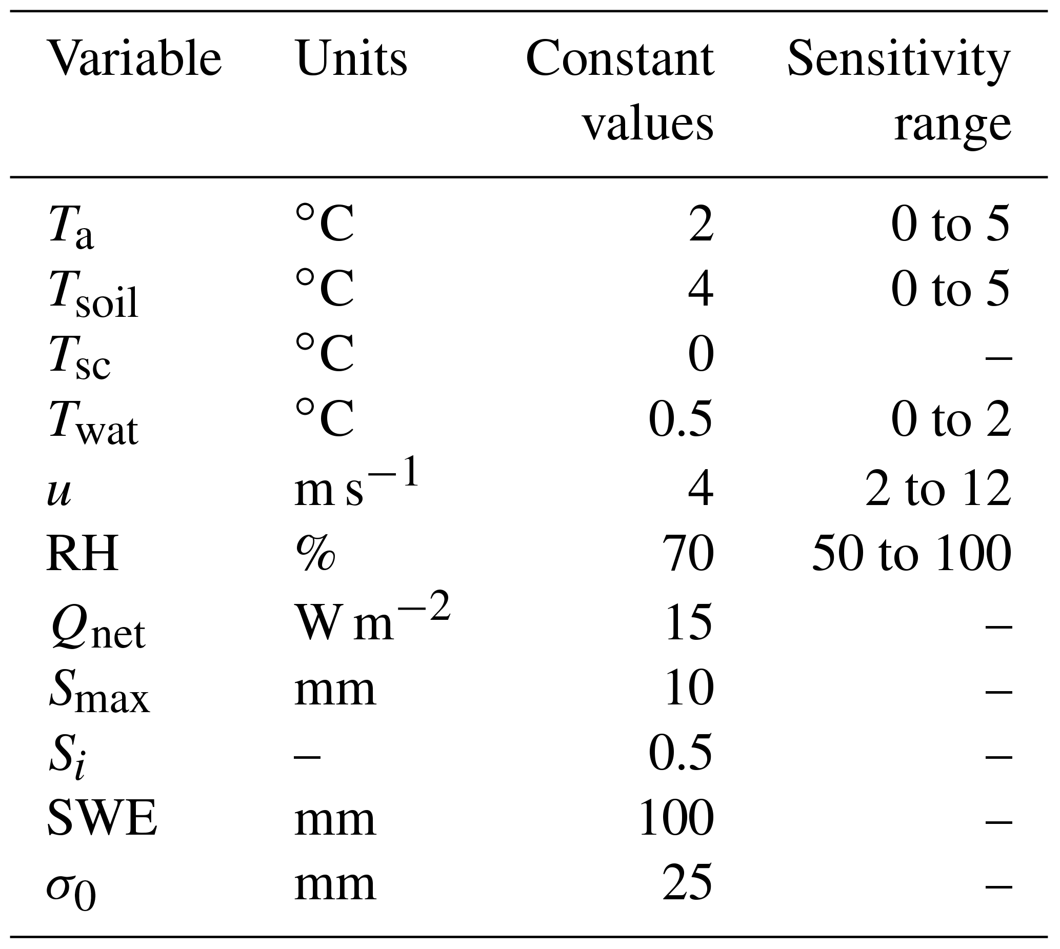
To explore the dynamics of modelled advection contributions several scenarios were implemented with the model. The first scenario (No Advection) constitutes a baseline for a typical one-dimensional model that assumes no advection, the second (dry surface) includes advection from a warm dry surface, the third (wet surface) includes advection from a warm wet surface, and the fourth (dry to wet surface) includes advection from a warm surface that transitions from dry to wet as a function of the INF–S_ret–F_water relationships. To understand the implications upon snowmelt for each scenario, input variables were held constant and the model was run until an assumed isothermal snowpack was fully depleted. A constant melt energy, Q_net (W m⁻²), was applied which represents the net snow surface energy balance as estimated via a typical one-dimensional model. The initialized SWE was ablated, leading to infiltration excess, detention-storage, runoff, or sublimation. The relative dynamics of the various scenarios are sensitive to the inputs and parameters used, as summarized in Table 2, and demonstrate the relationships between H_A and LE_A and the snow-free surface humidity conceptualization and snowmelt implications from a theoretical perspective.

2.3.2 Sensitivity analysis

The sensitivity of SLHAM to T_wat, T_a, T_soil, u, and RH variability is also explored to understand the implications upon SWE and SCA depletion, F_water, H_A, LE_A, and net advection. The dry to wet surface scenario, holding the input variables constant and varying each variable in turn as detailed in Table 2, was employed to understand the dynamics of input variability. A common assumption is that T_wat is 0 ^∘C as meltwater immediately after discharge from an isothermal snowpack is 0 ^∘C and underlying frozen soils are ≤0 ^∘C. Unlike the snow surface the maximum temperature of ponded water is unconstrained by phase change so values ≥0 ^∘C are expected because of possible low water surface albedos and high shortwave irradiance (SW${}_{\mathrm{atm}}^{\downarrow }$) during the daytime. Analysis of available thermal images from a FLIR T650 thermal camera was used to correct for atmosphere conditions and water surface emissivity. This analysis showed that daytime T_wat was generally >0 and <2 ^∘C. This range in T_wat was used to test the sensitivity of the T_wat upon SLHAM dynamics. Intermittency of observations and inherent uncertainties in thermography prevented a more precise estimation of T_wat. The ranges of all other variables were selected to represent conditions commonly experienced during snowmelt on the Canadian Prairies.

Table 2 Input variables for scenario analysis of SLHAM dynamics.

2.3.3 Coupled advection and snow–stubble–atmosphere snowmelt model simulations

Conditions controlling advection processes are not constant over snowmelt; therefore SLHAM was coupled with a one-dimensional snowmelt model (SSAM) to estimate the role of advection contributions over a snowmelt season. Briefly, SSAM describes the relationships between shortwave, longwave and turbulent exchanges between a snow surface underlying exposed crop stubble and the atmosphere. The surface energy balance was coupled to a single-layer snow model to estimate snowmelt. A slight modification of SSAM, or any one-dimensional model that computes areal average snowmelt, is needed to include advection. The energy terms of one-dimensional energy balance models are represented as flux densities (W m⁻²) over an assumed continuous snow cover and therefore need to be weighted by an SCA parametrization (Eq. 9) to properly simulate the areal average melt energy available to the fraction of the surface comprised of snow. The SSAM was run with and without SLHAM to explore the impact of advection simulation on SWE. Simulation performance was quantified via root mean square error (RMSE) and model bias (MB) of the simulated SWE versus snow survey SWE observations. The relative contribution of advection was quantified through estimation of the energy contribution to total snowmelt. A commonly used snowmelt model, the Energy Balance Snowmelt Model (EBSM) of Gray and Landine (1988), was also run to benchmark performance. The EBSM has been widely applied in this region and simulation is deployed as an option within the Cold Region Hydrological Modelling (CRHM) platform (Pomeroy et al., 2007).

The SSAM, SSAM–SLHAM and EBSM simulations were driven by common observed meteorological data, parameters and initial conditions obtained from intensive field campaigns at a research site near Rosthern, Saskatchewan, Canada (52.69^∘ N, 106.45^∘ W). The data for the 2015 and 2016 snowmelt seasons reflect relatively flat agricultural fields characterized by standing wheat stubble, with 15 and 24 cm stubble heights for the respective years. Observations of T_soil required for SLHAM come from infrared radiometers (Apogee SI-111) deployed on mobile tripods to snow-free patches. Unfortunately, no time series of T_wat observations are available and values or models to describe T_wat for shallow ponded meltwater in a prairie environment have not been discussed in the literature. Like snowpack refreezing, ponded meltwater can also refreeze at night as the heat capacity of this shallow water is limited. In this framework, as observations or models of T_wat are unavailable, a simple physically guided representation of T_wat takes the following form:

$$\begin{array}{}\text{(15)}& T_{\mathrm{wat}}=\begin{array}{ll}{T}_{\mathrm{sc}}& T_{\mathrm{sc}}<\mathrm{0}{}^{\circ }\mathrm{C},\\ \mathrm{0.5}{}^{\circ }\mathrm{C}& T_{\mathrm{sc}}=\mathrm{0}{}^{\circ }\mathrm{C}.\end{array}\end{array}$$

A description of the field site and data collection methodologies is detailed in Harder et al. (2018).

3 Results and discussion

3.1 Performance of extended GM2002

The extended GM2002 proposed here was tested using advection estimates from vertical air temperature and water vapour profiles as reported in Harder et al. (2017); the results are summarized in Table 3. The model slightly overestimated H_A and LE_A on 30 March 2015, likely due to the limiting assumptions of the GM2002 model. A key missing component of GM2002 is the influence of differences in surface roughness upon the growth of the internal boundary layer. A simple power law relationship with respect to distance from transition is employed in the model. Further work by Granger et al. (2006) demonstrated that boundary layer growth has a positive relationship with upwind surface roughness and that the parametrization employed in GM2002 overestimates the boundary layer depth, by up to a factor of 2 when upwind surface roughness is negligible. The GM2002 is based upon the integrated difference in temperature through the boundary layer depth; thus, a greater boundary layer depth will increase the estimated advection. This partly explains why the model overestimates values in the situation of a rough upwind surface. Other potential limiting assumptions include homogenous surface temperatures, uniform eddy diffusivities for different scalars, and no vertical advection. Despite the model limitations, the acceptable performance in simulating the 18 and 30 March observations gives confidence that this simple model is reasonable for some applications and provides guidance for future improvements.

Table 3 Model parameters, estimates and observations for evaluation of the extended GM2002.

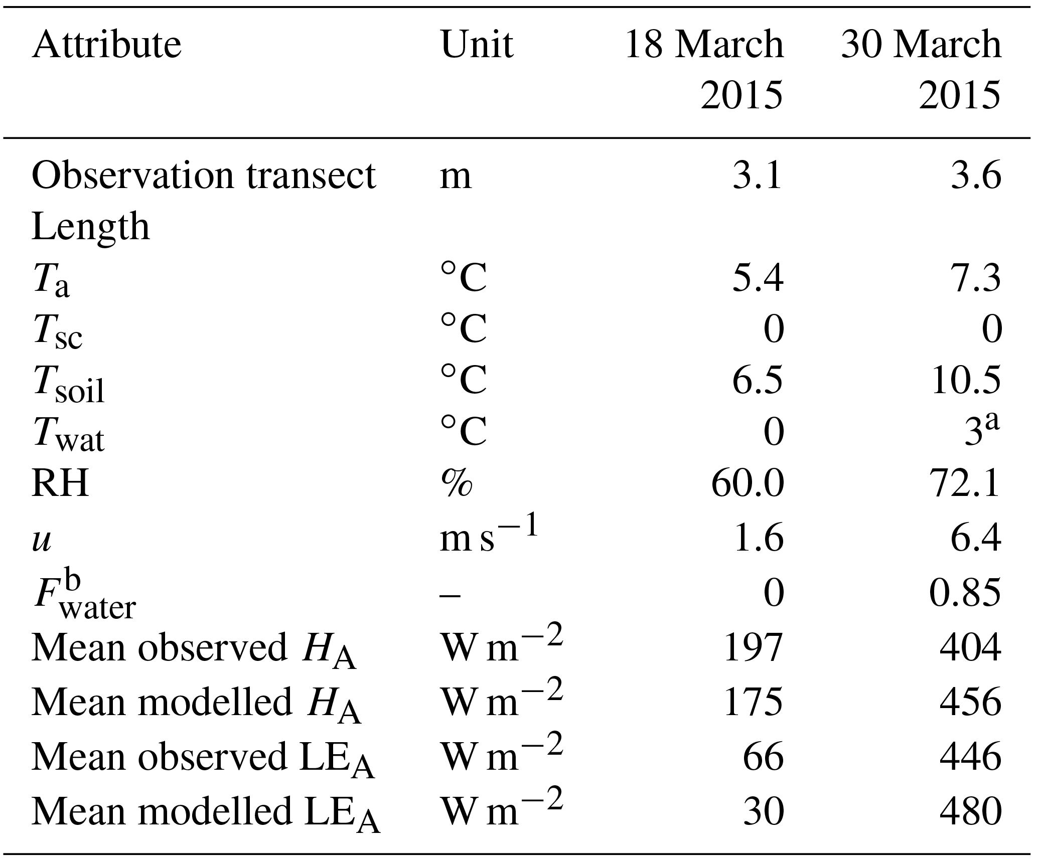
^a Estimated from thermography. ^b Roughly estimated from application of a 1 : 100 sensor height to flux footprint ratio (Hsieh et al., 2000) as applied to concurrent UAV imagery.

3.2 Re-evaluation of snow-cover geometry

Differences exist between the originally reported parameters and those found from the analysis of UAV imagery (mean coefficients summarized in Table 4). Early work applying fractal geometry to natural phenomena (Mandelbrot, 1975, 1982) discusses the Korcak exponent as a fractal dimension. More recent work suggests that the Korcak law describing the area–frequency relationship is not a fractal relationship but rather a mathematically similar, but distinct, scaling law (Imre and Novotn, 2016). Therefore, the D_k value is not necessarily ≥1 or ≤2 and the identified exponent terms in Table 4 near or greater than 2 are plausible. The D^′ terms are very similar to those previously reported (Granger et al., 2002). From this analysis, it is apparent that application of these parameters between sites must be done with caution as local topography and surface conditions may influence the snow patch size distribution. The lack of a temporal trend of these terms (time series of D_k in Fig. 6 and D^′ in Fig. 7) over the course of snowmelt and equivalence in scaling of snow and snow-free patches implies that locally specific parameters may be applied as constants over the course of the melt and irrespective of patch type. The resolution of the underlying imagery, differences in classification methodologies and surface characteristics may contribute to some of the differences in terms observed and those previously reported. An illustrative comparison is that of a tall and short stubble surface. The tall stubble surface snow-cover geometry is heavily influenced by the early exposure (and hence classification as non-snow from nadir imagery) of stubble rows, which leads to very long and narrow patches even if snow is still present within the stubble. In contrast the oblique imagery of Shook et al. (1993b) and Granger et al. (2002) will not quantify the snow between stubble rows and larger and less complex snow patches would be represented by the previously reported coefficients. Further work is needed to calculate the scaling properties of patches over a more comprehensive variety of topography and vegetation types.

Table 4 Updated mean snow-cover geometry parameters.

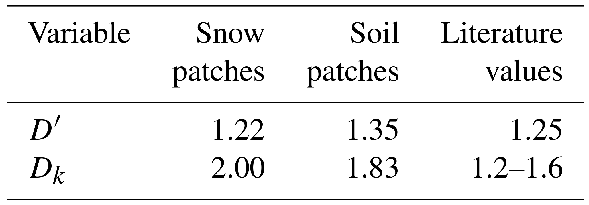
Figure 6 Time series of fitted D_k parameter with respect to snow and soil patches for various land covers over the course of snowmelt.

Figure 7 Time series of fitted D^′ parameter with respect to snow and soil patches for various land covers over the course of snowmelt.

3.3 Implications of including advection in snowmelt models

3.3.1 Advection dynamics in scenario simulations

The dynamics of the various scenarios are expressed through visualizations of SWE depletion (Fig. 8) and magnitudes of the H_A, LE_A and net advection terms (Fig. 9). A critical consequence of including SCA in snowmelt calculations is that areal average melt rates will vary between a continuous and heterogeneous snow surface. The Q_net driving melt in a one-dimensional melt model is in terms of a flux density; an energy flux with a unit area dimension (W m⁻²) where exchange is limited to the SCA. As the SCA decreases the corresponding areal average energy to melt snow will also decrease, which will decrease the areal average melt rate. This is evident in the melt rate of the No Advection scenario, which decreases with time as the SCA decreases. Including energy from advection, for the dry surface, wet surface, and dry to wet surface advection scenarios, causes the SWE to deplete faster as there is now an additional energy component that increases as SCA depletes. In these scenarios the additional energy gained from advection is greater than the reduction of areal average Q_net as SCA decreases. LE_A from a constant wet surface is greater than any other advection scenario. Despite a reduction in H_A from the cooler surface and therefore an overall slower melt, the consistently positive LE_A towards the snow leads to a large net advection flux. In contrast, a consistently warm dry surface has a much higher H_A flux, and faster melt rate, than the wet surface that is partly compensated by a negative LE_A due to sublimation and a decrease in the overall energy for melt from advection. When the surface wetness is parameterized by detention storage and frozen soil infiltration capacity, dry to wet surface, the snow-free surface is dry and warm in the early stages of melt and LE_A is negative and limits melt, as in the dry surface scenario. As melt proceeds and F_water begins to increase, the upwind T_sf cools and the humidity gradient switches, resulting in positive LE_A and a decrease in H_A, which compound to slow melt relative to the dry surface scenario. There are clear implications for the timing of melt and thus snow hydrology depending upon the upwind condition. It is evident that SLHAM can quantify the key advection behaviours in relation to the upwind surface dynamics.

Figure 8 Modelled snow water equivalent depletion for various advection scenarios.

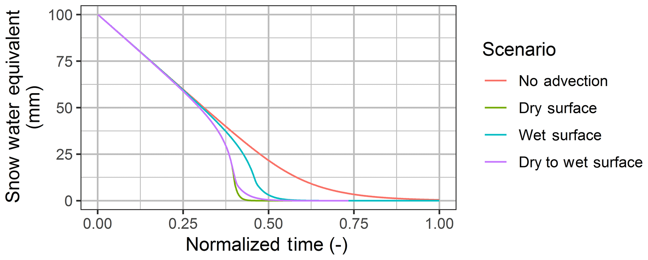
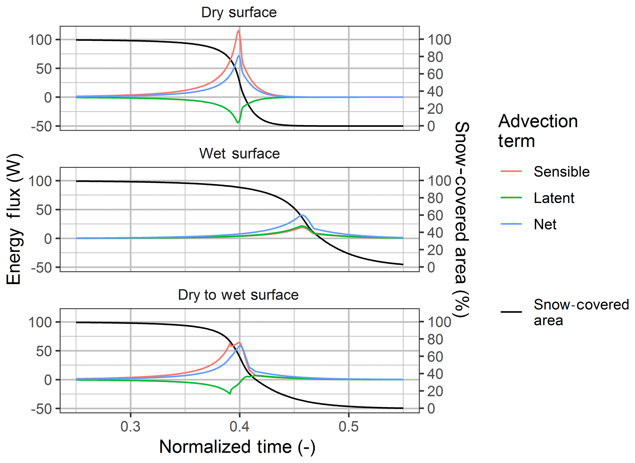
Figure 9 Latent heat (green), sensible heat (red) and net (blue) advection components for the SLHAM scenarios plotted with snow-covered area (black).

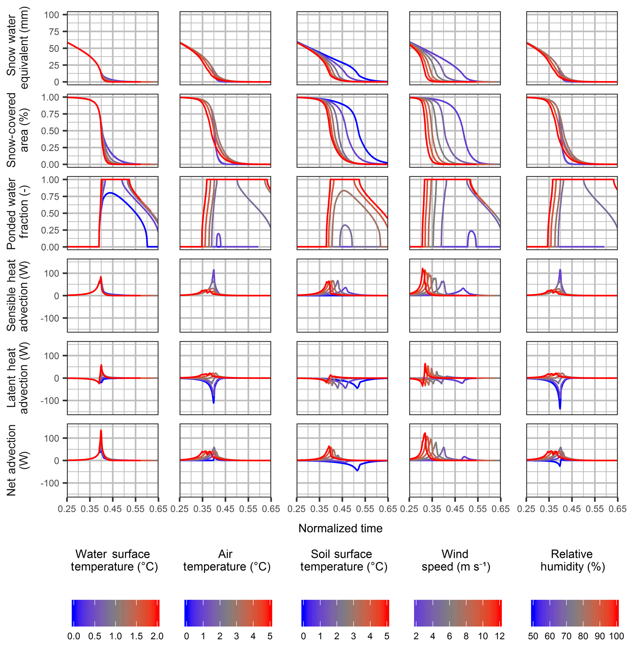
Figure 10 Sensitivity of snow water equivalent and snow-covered area depletion, ponded water fraction, sensible heat advection, latent heat advection and net advection with respect to variation in water surface temperature.

3.3.2 Sensitivity to input variables

The influence of the input variables on the SLHAM model is evaluated through a sensitivity analysis (Fig. 10). It is apparent from the variability in SWE depletion that the T_soil and u have the largest influence on advection contributions to snowmelt. This is expected as u and T_soil variables quantify the first-order controls driving advection, the air mass movement and horizontal scalar gradients respectively. In contrast the T_wat, T_a, and RH variables have considerably less variability for the ranges simulated as they have less influence upon the scalar profile differences between upwind and downwind locations. A critical model feedback relates to the influence dynamic upwind surface temperature and humidity and is articulated in this sensitivity analysis. If melt rates exceed the frozen soil infiltration capacity ponding occurs, F_water>0, which forces the upwind surface to the assumed water surface temperature. The consequent sign of the surface humidity gradient will influence whether LE_A induces condensation (increased melt rate) or sublimation (decreased melt rate), which influences the net advection and melt rate. This feedback is manifested in the sensitivity of all variables. The transition of the upwind surface from dry and warm to cooler and saturated tempers the advection contributions to melt. Generally, any change in a variable that increases the profile gradient or increases energy exchange will lead to increased SWE and SCA depletion rates and increased extent and duration of F_water. Changes in H_A and LE_A tend to be compensatory, resulting in relatively small increases in net advection fluxes.

Sensitivity to any variable is only expressed towards the end of the snowmelt, when SWE <50 mm and SCA is depleting rapidly. Differences in melt rate are limited by the rapid reduction in the SCA exchange surface at the end of snowmelt. Whilst clearly important for simulating the dynamics of advection and sources of energy driving snowmelt, T_wat, T_a, and RH have a relatively limited influence upon overall SWE depletion compared to T_soil and u. In the absence of T_wat models or observations, the assumptions outlined in Eq. (15) will have a relatively limited influence upon simulation of SWE with the fully coupled SSAM–SLHAM model.

3.3.3 Advection dynamics in coupled advection and snowmelt models

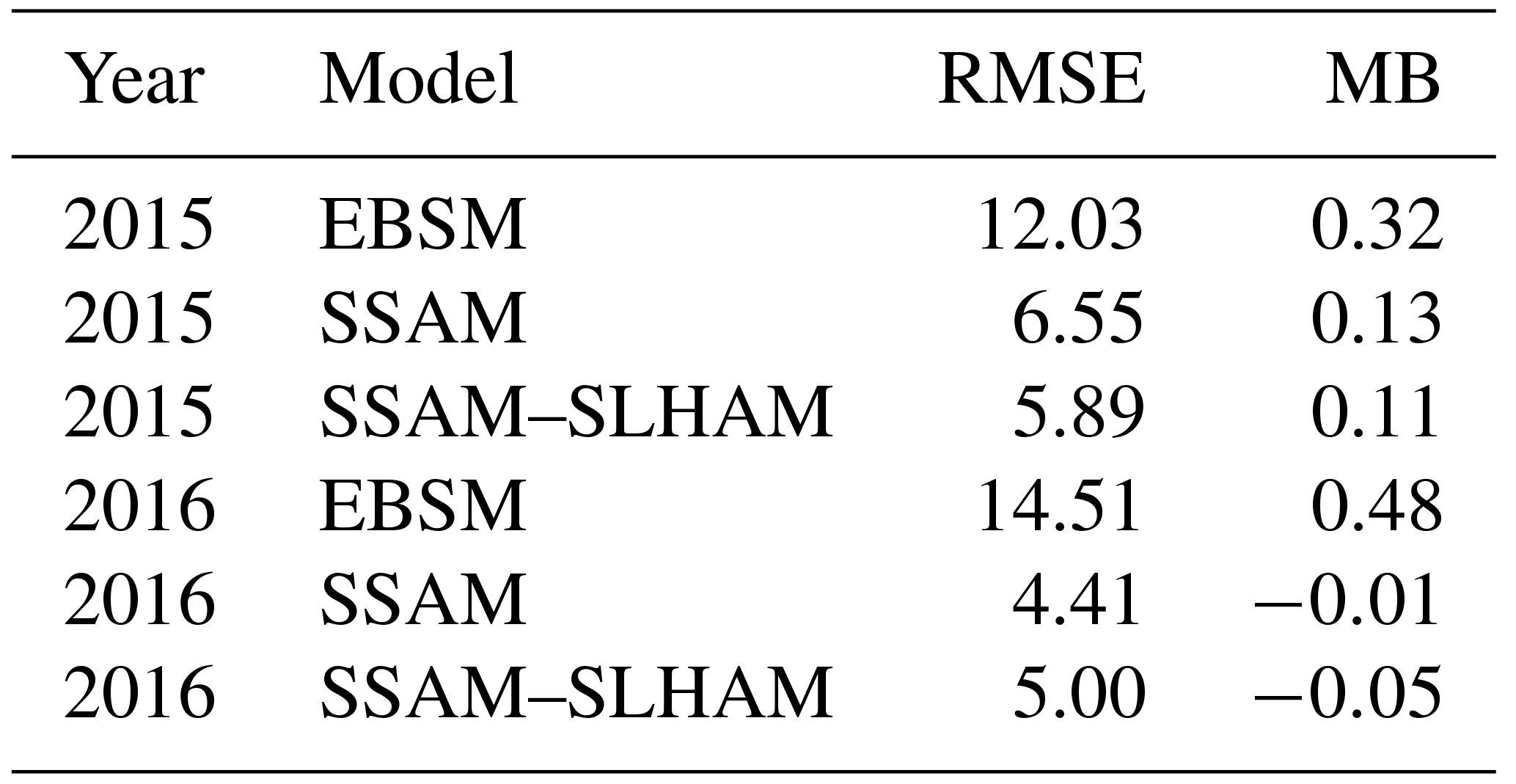
The scenario analysis demonstrates the melt response to variations in surface wetness but actual snowmelt situations have forcings that vary diurnally and with meteorological conditions. Snowmelt simulations with three models of varying complexity provide insight into the implications of process representation. SSAM and SSAM–SLHAM show considerable improvement when compared to EBSM (Fig. 11 and Table 5). The SSAM simulation is by itself a significant improvement upon EBSM for SWE prediction during melt. The addition of SLHAM does not change the SWE simulation performance appreciably but does increase the physical realism of the model with its more complete surface energy balance. The SSAM–SLHAM simulations including advection, relative to SSAM simulations without advection, led to lower areal average melt rates in 2015 and higher rates in 2016. Lower wind speeds in 2015 led to lower advection contributions than 2016, which had relatively higher wind speeds. The comparison of the simulated melt with snow survey SWE observations showed that the differences are minimal (Fig. 11 and Table 5). While the SSAM–SLHAM simulations do not change melt rates or total amount of energy, the sources of energy driving snowmelt do change. Early melt displays no differences as SCA remains relatively homogenous. Differences appear due to decreases in the turbulent radiation fluxes, with a decrease in the SCA exchange surface due to increases in advection fluxes with increasing horizontal scalar gradients and surface heterogeneity. The cumulative net energy from advection for these two seasons contributed energy to melt 4 and 5 mm of SWE in 2015 and 2016, respectively (Fig. 12). The advection energy contribution represents 6.5 % and 10.6 % of total snowmelt in 2015 and 2016, respectively.

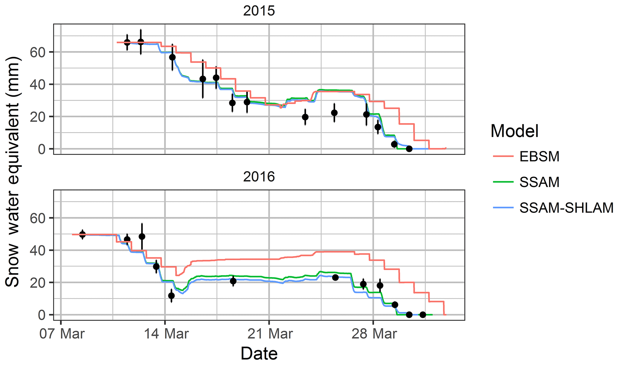
Figure 11 Snow water equivalent simulation for EBSM (red line), SSAM (green line) and SSAM–SLHAM (blue line) with respect to snow survey mean (black points) and 95 % percentile sampling confidence interval (black lines).

Table 5 Error metrics of snow water equivalent simulation versus snow survey observations for EBSM, SSAM and SSAM–SLHAM models.

3.4 Energy balance compensation

An unappreciated dynamic of local-scale advection during snowmelt is that LE_A and H_A may be of opposite sign and therefore will compensate for one another, leading to a lower net advection contribution. This occurs when the gradients of T and q between a snow-free and snow-covered surface are opposite in sign; a warm but dry snow-free surface upwind of a cool and wet snow-covered surface driving snow surface sublimation. This was evident in the reduction of the advection energy due to a negative LE_A throughout the dry surface scenario and early melt of the dry to wet surface scenario (Fig. 9). In the 2015 and 2016 snowmelt simulations, the accumulated LE_A was negative for much of the melt period, which compensated for the consistently positive H_A term (Fig. 12). LE_A only increased, enhancing the positive H_A contribution, near the end of melt in 2015 when increased surface wetness led to a positive LE_A term.

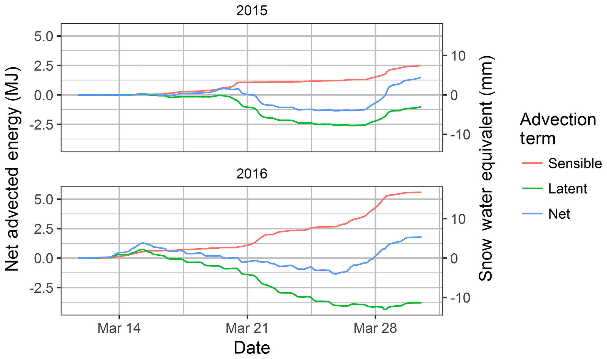
Figure 12 Cumulative sensible (red), latent (green) and net (blue) advection terms in terms of energy (MJ: left) and equivalent melted snow water equivalent (mm SWE: right axis).

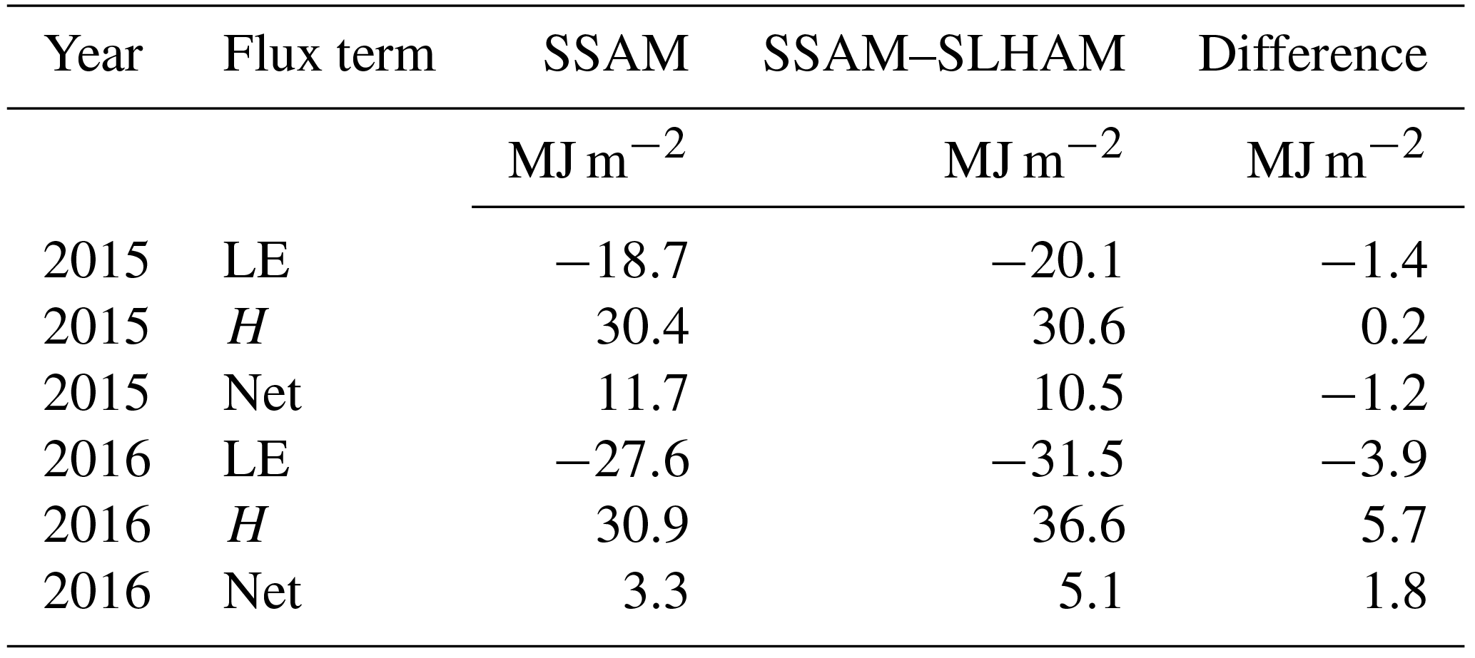
The advection fluxes may also be of opposite sign to the sensible (H_snow) and latent (LE_snow) turbulent fluxes between the snow surface and the atmosphere. Inclusion of the advection process therefore influences the overall sensible and latent heat exchange at the snow surface (net exchange). This interaction is further complicated by the varying SCA of the SSAM–SLHAM model versus the complete snow cover assumption of SSAM. Including advection decreased cumulative LE by 1.4 MJ in 2015 and by 3.9 MJ in 2016 (Table 6). Cumulative H, when including advection, increased by 0.2 MJ in 2015 and by 5.7 MJ in 2016. The net exchange when including advection shows that the inclusion of LE_A decreases the influence of H_A; the change in net exchange is lower than the change in H exchange (Table 6). The role of advection in modifying net exchange is clearly complex and varies by season. Despite differences in magnitude, the opposite signs of LE_A and H_A demonstrate that these energy contributions partially compensate for one another, therefore reducing the net influence of advection on snowmelt. This compensatory relationship has been missed by the focus on H_A in snowmelt advection research, which has therefore overemphasized the contribution of H_A to snowmelt. This compensatory mechanism also helps to explain why observed latent heat fluxes are often much smaller than model predictions in the meltwater-ponded Canadian Prairies during melt (Granger et al., 1978). The compensation of H_A by LE_A will be a more important interaction on the Canadian Prairies, or similar level environments, but perhaps less so in mountain regions where complex terrain leads to rapid meltwater runoff.

Table 6 Cumulative energy from sensible, latent and net exchange for 2015 and 2016 snowmelt simulations with (SSAM–SLHAM) and without (SSAM) advection.

3.5 To advect or not to advect?

The simulation of snowmelt with, and without, advection gave minimal differences in the resulting SWE simulation. This demonstrates system insensitivity to processes that on their own appear to be important. This may explain why EBSM, like many other physically based snowmelt models (Jordan, 1991; Lehning et al., 1999; Marks et al., 1998), does not accommodate heterogeneous snow cover yet successfully simulates SWE depletion. In EBSM the simulation of an areal average albedo rather than a snow albedo performed relatively well in simulating SWE (Fig. 11) without considering SCA depletion or advection controls. The modelling challenges of a_snow are not limited to EBSM as other a_snow parameterizations, especially temperature-dependent ones, typically underestimate a_snow during melt and therefore indirectly, and perhaps unintentionally, account for advected energy contributions (Pedersen and Winther, 2005; Raleigh et al., 2016). While modelled a_snow values that underestimate actual a_snow values are effective parameterizations for simulation of SWE, they cannot realistically incorporate the impacts of dust on snow or changes in snow albedo with grain size or wetness. Hence, SCA constraints and advection process conceptualizations are necessary to improve confidence in and applicability of snowmelt models. This is evident when comparing the more accurate and physically complete SSAM–SLHAM simulation of SWE to the EBSM simulation of SWE (Fig. 11).

Understanding the implications of land-use and climate changes on variables beyond SWE are needed to fully inform coupled modelling of land–atmosphere and radiation feedbacks between land surface and numerical weather or climate models. The framework presented explicitly considers advection and scales it with SCA, u and horizontal gradients, which are the primary controls of advection. A simple indication that a more appropriate model conceptualization is being used in this advection framework is that the minimum albedo value simulated is 0.75. This is consistent with that for clean, melting snow (Wiscombe and Warren, 1980), whilst the 0.2 in EBSM is not. While the SWE simulation differences are not particularly large, the new model is getting the “right” answer for the “right” reasons and without calibration. By including a more appropriate suite of physical processes, this model can produce realistic melt simulations in areas or years where the variables governing advection deviate from the conditions observed during model development.

3.6 Limitations and future research needs

The SLHAM framework replaces the large uncertainty deriving from physically unrealistic albedo parametrizations (Gray and Landine, 1987; Raleigh et al., 2016) and ignored SCA dynamics (Essery and Pomeroy, 2004) with a more physically realistic framework. The individual process parametrizations still have uncertainties that need to be constrained. The advection versus patch length parametrization of GM2002 lacks inclusion of surface roughness differences and the valid bounds of the parametrizations need clarification. Observations of stable atmospheric profiles over snow patches (Fujita et al., 2010; Mott et al., 2015, 2016; Shook and Gray, 1997) complicate energy exchange. The goal of this simple model was to develop an easy-to-implement advection framework with stability represented by the Weisman (1977) stability parameters. Future work will need to revaluate the stability assumptions of Granger et al. (2002) and Weisman (1977) or devise more appropriate schemes to account for the stability influence. The SCA model of Essery and Pomeroy (2004) is challenged by exposure of vegetation in shallow snow. The conceptual surface water ponding model developed in this work requires field observations or further parameterizations to accurately quantify the relevant variables. The transition of advection mechanism from snow-free sources to snow patch sources uses a conceptualized relationship to SCA. A targeted field campaign is needed to assess the validity of the conceptualized f_s and its possible relation to the advection efficiency term of Marsh and Pomeroy (1996). An estimate of T_sf is needed to implement this framework and will limit application of SLHAM in its current form, as modelling T_sf is non-trivial and observations are often unavailable. Ideally a multisource land surface scheme with explicit representation of soils and ponded water is used to represent T_soil and T_wat. In the interim, the T_wat assumptions in Eq. (15) may be used but need to be tested further. A regression of T_soil to incoming shortwave radiation and T_a is presented in the Appendix to provide a simple and physically guided solution to remove this limitation when modelling snowmelt in agricultural regions on the Canadian Prairies. These uncertainties will be addressed in future work and will require additional field observations and model validation, testing, or development.

4 Conclusions

To date, the development of easily implementable and appropriate models to estimate the advection of H_A and LE_A to snow during melt has proved elusive. The formulation presented here is an initial framework that can be used to augment existing one-dimensional snowmelt models. When tested against observations the extended GM2002 model provides reasonable estimates of both H_A and LE_A and opportunities for improvement of the method are discussed. The scaling parameters necessary to describe the spatial heterogeneity of snow and snow-free patches were re-evaluated with UAV data. Coupling of the simple advection model with snow-cover geometry scaling laws, SCA depletion, frozen soil infiltration and a surface detention fractional water area parameterization resulted in a model that meets the objective of a formulation that can account for LE_A and H_A to snow as an areal average contribution. A scenario-based analysis of the model revealed the compensatory influence of LE_A from a warm but dry surface; the LE_A-driven sublimation offsets H_A inputs. Coupling SLHAM with SSAM demonstrated that advection constitutes an important portion of melt energy: 11 % of the melt observed in the 2016 snowmelt season. The reduced radiation exchange to the snow surface fraction, due to decreasing SCA, is compensated for with an increase in net sensible and latent heat exchange that leads to minimal differences in the SWE depletion. This compensatory dynamic has sometimes allowed one-dimensional energy balance snowmelt models to provide adequate simulation of SWE despite using the “wrong” process conceptualizations. The advection model framework proposed here can be easily coupled to existing one-dimensional energy balance models and is expected to improve the prediction of snowmelt in areas dominated by heterogeneous snow cover during melt. Such adoption will permit successful use of more realistic albedo parameterizations. This work provides a guiding framework to address the long-identified need to develop “bulk methodologies” for calculating sensible and latent heat terms for patchy snow-cover conditions (Gray et al., 1986).

Appendix A

The SLHAM framework requires a T_soil value which is a challenging variable to explicitly model during snowmelt. To provide an interim solution a multiple linear regression is developed to estimate T_soil from SW${}_{\mathrm{atm}}^{\downarrow }$ and T_a. This empirical parameterization is appropriate to the snowmelt situation on the Canadian Prairies when the surface is comprised of crop residues and should be treated with caution in other domains. The developed regression is physically guided as the main variables controlling T_soil is the net radiation, whose variability is dominated by SW${}_{\mathrm{atm}}^{\downarrow }$, and turbulent fluxes, which are dependent upon the T_a gradients. During nighttime T_soil is very similar to T_a while during daytime the additional energy from SW${}_{\mathrm{atm}}^{\downarrow }$ heats the surface to temperatures above T_a. A multiple regression that contains these parameters provides a simple but effective way to estimate T_soil in a manner consistent with energy balance interactions. A full description of the observations used to parameterize this relationship can be found in Harder et al. (2018). Briefly the T_a is observed with a shielded Campbell Scientific HMP45C212 and SW${}_{\mathrm{atm}}^{\downarrow }$ is observed with a Campbell Scientific CNR1 with both sensors 2 m above the ground surface. The T_soil observations from Apogee SI-111 sensors, mounted on mobile tripods to ensure consistent representation snow-free surfaces, sampled surfaces of tall wheat stubble (0.35 m) and short wheat stubble (0.2 m) in 2015 and wheat stubble (0.24 m) and canola stubble (0.24 m) in 2016. Hereafter they are referred to as tall stubble, short stubble, wheat and canola, respectively. All observations were logged at 15 min intervals. The empirical representation of T_soil (^∘C) in relation to SW${}_{\mathrm{atm}}^{\downarrow }$ (W m⁻²) and T_a (^∘C) is

$$\begin{array}{}\text{(A1)}& T_{\mathrm{soil}}=\mathrm{0.00339}{\mathrm{SW}}_{\mathrm{atm}}^{\downarrow }+\mathrm{0.977}{T}_{\mathrm{a}}-\mathrm{1.22}.\end{array}$$

Model performance was assessed with the root mean square error (RMSE) and model bias (MB). Each test provides a different perspective on model performance: RMSE is a weighted measure of the difference between the observation and model (Legates and McCabe, 2005), and MB indicates the mean over- or underprediction of the model versus observations (Fang and Pomeroy, 2007). The T_soil regression provides good estimates of the diurnal variability and magnitudes with respect to observations (Fig. A1). The highest values during daytime are simulated well, which is critical for the appropriate simulation of advection processes. There is low bias for all simulations; MB < 1.09 ^∘C. The RMSEs between 1.39 and 1.94 ^∘C are negligible as most surface temperature models will simulate errors at a similar magnitude (Aiken et al., 1997). This parametrization provides a simple but effective workaround if T_soil observations are unavailable or unmodelled. This empirical relation should be treated with caution if implemented outside of the conditions found during snowmelt in cropland areas of the Canadian Prairies. In such cases locally derived relationships should be developed or T_soil should be explicitly modelled.

Figure A1 Soil surface temperature observed versus modelled as scatter plots (a) and time series (b).