A dimensionless approach for the runoff peak assessment: effects of the rainfall event structure

The present paper proposes a dimensionless analytical framework to investigate the impact of the rainfall event structure on the hydrograph peak. To this end a methodology to describe the rainfall event structure is proposed based on the similarity with the depth–duration–frequency (DDF) curves. The rainfall input consists of a constant hyetograph where all the possible outcomes in the sample space of the rainfall structures can be condensed. Soil abstractions are modelled using the Soil Conservation Service method and the instantaneous unit hydrograph theory is undertaken to determine the dimensionless form of the hydrograph; the two-parameter gamma distribution is selected to test the proposed methodology. The dimensionless approach is introduced in order to implement the analytical framework to any study case (i.e. natural catchment) for which the model assumptions are valid (i.e. linear causative and time-invariant system). A set of analytical expressions are derived in the case of a constant-intensity hyetograph to assess the maximum runoff peak with respect to a given rainfall event structure irrespective of the specific catchment (such as the return period associated with the reference rainfall event). Looking at the results, the curve of the maximum values of the runoff peak reveals a local minimum point corresponding to the design hyetograph derived according to the statistical DDF curve. A specific catchment application is discussed in order to point out the dimensionless procedure implications and to provide some numerical examples of the rainfall structures with respect to observed rainfall events; finally their effects on the hydrograph peak are examined.

1 Introduction

The ability to predict the hydrologic response of a river basin is a central feature in hydrology. For a given rainfall event, estimating rainfall excess and transforming it to a runoff hydrograph is an important task for planning, design and operation of water resources systems. For these purposes, design storms based on the statistical analysis of the annual maximum series of rainfall depth are used in practice as input data to evaluate the corresponding hydrograph for a given catchment. Several models are documented in the literature to describe the hydrologic response (e.g. Chow et al., 1988; Beven, 2012): the simplest and most successful is the unit hydrograph concept first proposed by Sherman (1932). Due to a limited availability of observed streamflow data mainly in small catchment, the attempts in improving the peak flow predictions have been documented in the literature since the last century (e.g. Henderson, 1963; Meynink and Cordery, 1976) to date. Recently, Rigon et al. (2011) investigated the dependence of peak flows on the geomorphic properties of river basins. In the framework of flood frequency analysis, Robinson and Sivapalan (1997) presented an analytical description of the peak discharge irrespective of the functional form assumed to describe the hydrologic response. Goel et al. (2000) combine a stochastic rainfall model with a deterministic rainfall–runoff model to obtain a physically based probability distribution of flood discharges; results demonstrate that the positive correlation between rainfall intensity and duration impacts the flood flow quantiles. Vogel et al. (2011) developed a simple statistical model in order to simulate observed flood trends as well as the frequency of floods in a nonstationary context including changes in land use, climate and water uses. Iacobellis and Fiorentino (2000) proposed a derived distribution of flood frequency, identifying the combined role played by climatic and physical factors on the catchment scale. Bocchiola and Rosso (2009) developed a derived distribution approach for flood prediction in poorly gauged catchments to shift the statistical variability of a rainfall process into its counterpart in terms of statistical flood distribution. Baiamonte and Singh (2017) investigated the role of the antecedent soil moisture condition in the probability distribution of peak discharge and proposed a modification of the rational method in terms of a priori modification of the rational runoff coefficients.

In this framework, the present research study takes a different approach by exploring the role of the rainfall event features on the peak flow rate values. Therefore the main objective is to implement a dimensionless analytical framework that can be applied to any study case (i.e. natural catchment) in order to investigate the impact of the rainfall event structure on hydrograph peak. Since the catchment hydrologic response and in particular the hydrograph peak is subjected to a very broad range of climatic, physical, geomorphic and anthropogenic factors, the focus is posed on catchments where lumped rainfall–runoff models are suitable for deterministic event-based analysis. In the proposed approach, the rainfall event structure is described by investigating the maximum rainfall depths for a given duration d in the range of durations [$d/\mathrm{2};\mathrm{2}d$] within that specific rainfall event, differently from the statistical analysis of the extreme rainfall events. Other authors (e.g. Alfieri et al., 2008) have previously discussed the accuracy of literature design hyetographs (such as the Chicago hyetograph) for the evaluation of peak discharges during flood events; conversely the proposed methodology allows the investigation of the impact of the above-mentioned rainfall event structure on the magnification of the runoff peak neglecting the expected rainfall event features condensed in the depth–duration–frequency (DDF) curves.

The first specific objective is to define a structure relationship of the rainfall event able to describe the sample space of the rainfall event structures by means of a simple power function. The second specific objective is to implement a dimensionless approach that allows the generalization of the assessment of the hydrograph peak irrespective of the specific catchment characteristic (such as the hydrologic response time, the variability of the infiltration process, etc.), thus focusing on the impact of the rainfall event structure.

Finally a specific catchment application is discussed in order to point out the dimensionless procedure implications and to provide some numerical examples of the rainfall structures with respect to observed rainfall events; furthermore their effects on the hydrograph peak are examined.

2 Methodology

A dimensionless approach is proposed in order to define an analytical framework that can be applied to any study case (i.e. natural catchment). It follows that both the rainfall depth and the rainfall–runoff relationship, which are strongly related to the climatic and morphologic characteristics of the catchment, are expressed through dimensionless forms. In this paper, [L] refers to length and [T] refers to time.

The rainfall event is then described as constant hyetographs of a given durations; this simplification is consistent with the use of deterministic lumped models based on the linear system theory (e.g. Bras, 1990). The proposed approach is therefore valid within a framework that assumes that the watershed is a linear causative and time-invariant system, where only the rainfall excess produces runoff. In detail, the rainfall–runoff processes are modelled using the Soil Conservation Service (SCS) method for soil abstractions and the instantaneous unit hydrograph (IUH) theory. Consistently with the assumptions of the UH theory, the proposed approach is strictly valid when the following conditions are maintained: the known excess rainfall and the uniform distribution of the rainfall over the whole catchment area.

2.1 The dimensionless form of the rainfall event structure function

Rainfall DDF curves are commonly used to describe the maximum rainfall depth as a function of duration for given return periods. In particular for short durations, rainfall intensity has often been considered rather than rainfall depth, leading to intensity–duration–frequency (IDF) curves (Borga et al., 2005). Power laws are commonly used to describe DDF curves in Italy (e.g. Burlando and Rosso, 1996) and elsewhere (e.g. Koutsoyiannis et al., 1998). The proposed approach describes the internal structure of rainfall events based on the similarity with the DDF curves. Referring to a rainfall event, the maximum rainfall depth observed for a given duration is described in terms of a power function similarly to the DDF curve, as follows:

$$\begin{array}{}\text{(1)}& h\left(d\right)=a^{\prime }{d}^n,\end{array}$$

where h [L] is the maximum rainfall depth, a^′ [LT⁻ⁿ] and n [–] are respectively the coefficient and the structure exponent of the power function for a given duration, d [T]. For each duration d_i, the corresponding power function exponent, n, is estimated based on the maximum rainfall depth values observed in the range of duration [$d/\mathrm{2};\mathrm{2}d$] by means of a simple linear regression analysis. Based on such assumptions, the structure exponent n allows the description of the rainfall event based on a simple rectangular hyetograph, thus representing the rainfall event structure at a given duration. In other words, a rainfall event that is characterized by a specific n-structure exponent at a given duration is only one of the possible outcomes in the sample space of the rainfall structures. The n-structure exponent mathematically ranges between 0 and 1: the two extreme values represent unrealistic events characterized by opposite internal structure; when the structure exponent n tends to zero the internal structure of the rainfall event is comparable to a Dirac impulse while it is comparable to a constant intensity rainfall for n close to 1. As an example, Fig. 1 describes the rainfall event structure according to the approach illustrated above. In Fig. 1, the observed rainfall depth (at the top), the observed maximum rainfall depths (at the centre) and the corresponding rainfall structure exponent (at the bottom) are reported on hourly basis.

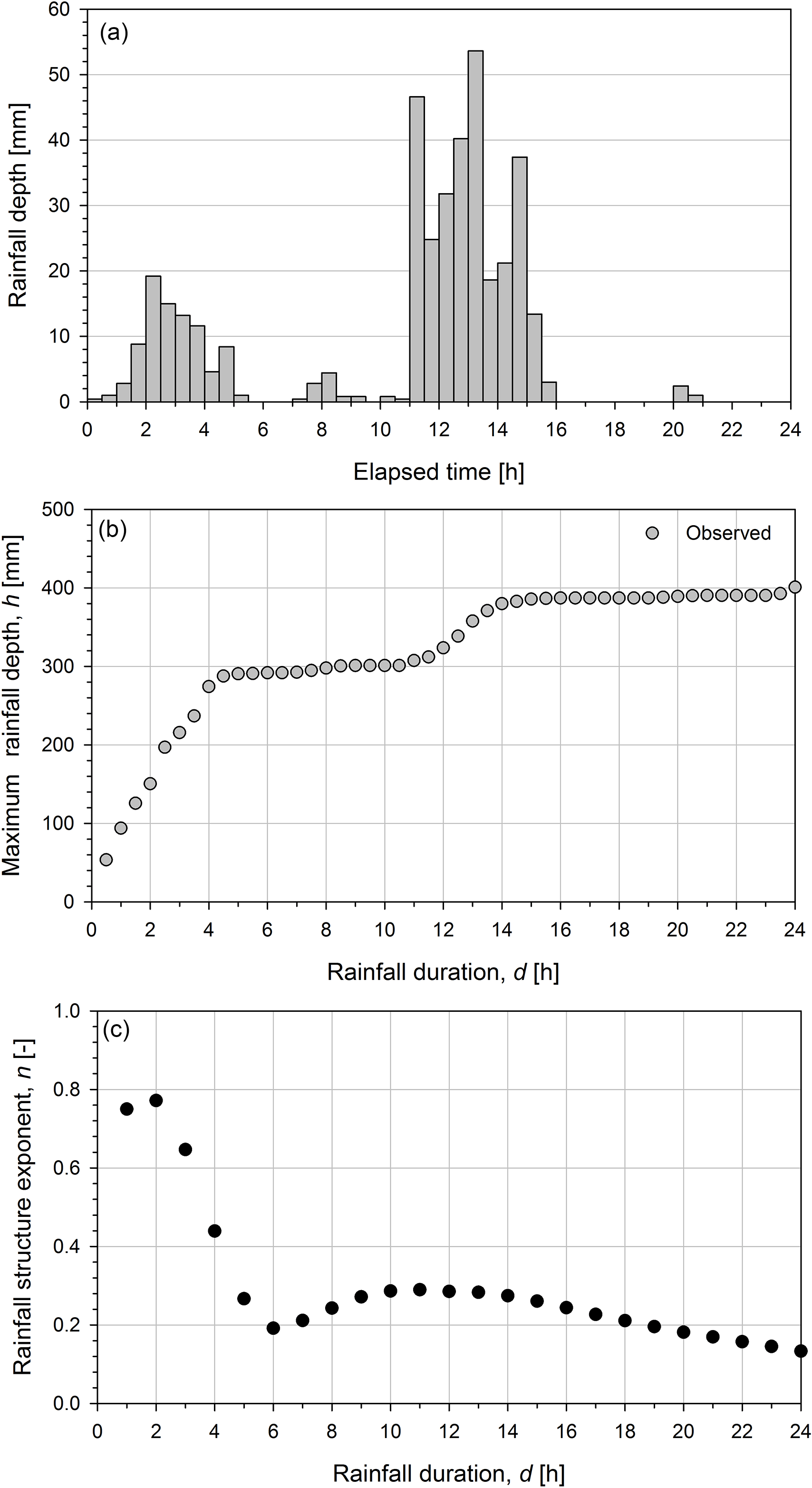
Figure 1 Rainfall event structure: the observed rainfall depth (a), the observed maximum rainfall depths (b) and the corresponding rainfall structure exponent (c) are reported.

In order to correlate the rainfall event structure function to the DDF curve, a reference rainfall event has to be defined in terms of the maximum rainfall depth, h_r, occurring for the reference duration, t_r. Focusing on a given catchment, the reference duration, t_r, is assumed to be equal to the hydrologic response time of the catchment; thus, assuming a specific return period T_r [T], the reference value of the maximum rainfall depth, h_r [L], is defined according to the corresponding DDF curves, as follows:

$$\begin{array}{}\text{(2)}& h_{\mathrm{r}}(T_{\mathrm{r}},t_{\mathrm{r}})=a\left(T_{\mathrm{r}}\right)t_{\mathrm{r}}^b,\end{array}$$

where a(T_r) [LT^−b] and b [–] are respectively the coefficient and the scaling exponent of the DDF curve.

Referring to a rainfall duration corresponding to t_r, the rainfall depth is assumed to be equal to the reference value of the maximum rainfall depth. Based on this assumption a relationship between the parameters of the DDF curve and the rainfall event structure function can be derived as follows:

$$\begin{array}{}\text{(3)}& h\left(t_{\mathrm{r}}\right)=h_{\mathrm{r}}\left(T_{\mathrm{r}},t_{\mathrm{r}}\right)\to a^{\prime }{t}_{\mathrm{r}}^n=a\left(T_{\mathrm{r}}\right){t_{\mathrm{r}}}^b\to {\displaystyle \frac{a^{\prime }}{a\left(T_{\mathrm{r}}\right)}}={\displaystyle \frac{t_{\mathrm{r}}^b}{t_{\mathrm{r}}^n}}.\end{array}$$

From Eq. (3) it is possible to derive the coefficient of the rainfall event structure function, a^′, for a given reference duration, t_r. Note that the a^′ coefficient is assumed to be valid in the range [$t_{\mathrm{r}}/\phantom{t_{\mathrm{r}}\mathrm{2}}\mathrm{2};\mathrm{2}{t}_{\mathrm{r}}$] similarly to the n-structure exponent.

The dimensionless approach is then introduced since it allows an analytical framework to be defined which can be applied to any study case (i.e. natural catchment) for which the model assumptions are valid (i.e. linear causative and time-invariant system). The reference values h_r and t_r are directly linked to the climatic and morphologic characteristics of the specific catchment, and therefore the dimensionless approach based on the h_r and t_r values allows the generalization of the results irrespective of the specific catchment characteristic (such as the return period associated with the reference rainfall event).

Based on the proposed approach, the dimensionless form of the rainfall depth, h_∗, is defined by the ratio of the rainfall depth, h, to the reference value of the maximum rainfall depth, h_r; similarly the dimensionless duration, d_∗, is expressed by the ratio of the duration, d, to the reference time, t_r. Therefore, the dimensionless form of the rainfall structure relationship may be expressed utilizing Eqs. (1), (2) and (3):

$$\begin{array}{}\text{(4)}& h_{\ast }\left(d_{\ast }\right)={\displaystyle \frac{h}{h_{\mathrm{r}}}}={\displaystyle \frac{a^{\prime }{d}^n}{a\left(T_{\mathrm{r}}\right){t_{\mathrm{r}}}^b}}={\displaystyle \frac{d^n}{t_{\mathrm{r}}^n}}=d_{\ast }^n.\end{array}$$

2.2 The dimensionless form of the unit hydrograph

The hydrologic response of a river basin is here predicted through a deterministic lumped model: the interaction between rainfall and runoff is analysed by viewing the catchment as a lumped linear system (Bras, 1990). The response of a linear system is uniquely characterized by its impulse response function, called the instantaneous unit hydrograph. For the IUH, the excess rainfall of unit amount is applied to the drainage area in zero time (Chow et al., 1988).

To determine the dimensionless form of the unit hydrograph a functional form for the IUH and thus the S-hydrograph has to be assumed. In this paper the IUH shape is described with the two-parameter gamma distribution (Nash, 1957):

$$\begin{array}{}\text{(5)}& {\displaystyle }f\left(t\right)={\displaystyle \frac{\mathrm{1}}{k\mathrm{\Gamma }\left(\mathit{\alpha }\right)}}{\left({\displaystyle \frac{t}{k}}\right)}^{\mathit{\alpha }-\mathrm{1}}{e}^{-\left(\frac{t}{k}\right)},\end{array}$$

where f(t) [T⁻¹] is the IUH, Γ [–] is the gamma function, α [–] is the shape parameter and k [T] is the scale parameter. In the well-known two-parameter Nash model, the parameters α and k represent the number of linear reservoirs added in series and the time constant of each reservoir, respectively. The product αk is the first-order moment, thus corresponding to the mean lag time of the IUH. Note that the IUH parameters can be related to the watershed geomorphology; in these terms the geomorphologic unit hydrograph (GIUH) theory attempts to relate the IUH of a catchment to the geometry of the stream network (e.g. Rodriguez-Iturbe and Valdes, 1979; Rosso, 1984). The use of the Nash IUH allows an analytical framework to be defined which assesses the relationship between the maximum dimensionless peak and the n-structure exponent for a given dimensionless duration, and similar analytical derivation can be carried out for simple synthetic IUHs. The dimensionless form of the IUH is obtained by using the dimensionless time, t_∗, defined as follows:

$$\begin{array}{}\text{(6)}& t_{\ast }={\displaystyle \frac{t}{\mathit{\alpha }k}}.\end{array}$$

The proposed dimensionless approach is based on the use of the IUH scale parameter as the reference time of the hydrologic response (i.e. t_r=αk). Using the first-order moment in the dimensionless procedure, the proposed approach can be applied to any IUH form even if, for experimentally derived IUHs, the analytical solution of the problem is not feasible.

By applying the change of variable $t=\mathit{\alpha }k{t}_{\ast }$, the IUH may be expressed as follows:

$$\begin{array}{}\text{(7)}& {\displaystyle }f\left(t\right)={\displaystyle \frac{\mathrm{1}}{k\mathrm{\Gamma }\left(\mathit{\alpha }\right)}}{\left({\displaystyle \frac{\mathit{\alpha }k{t}_{\ast }}{k}}\right)}^{\mathit{\alpha }-\mathrm{1}}{e}^{-\left(\frac{\mathit{\alpha }k{t}_{\ast }}{k}\right)}.\end{array}$$

The dimensionless form of the IUH, f(t_∗), is defined and derived from Eq. (7) as follows:

$$\begin{array}{}\text{(8)}& {\displaystyle }f\left(t_{\ast }\right)=f\left(t\right)\cdot \mathit{\alpha }k={\displaystyle \frac{\mathit{\alpha }}{\mathrm{\Gamma }\left(\mathit{\alpha }\right)}}{\left(\mathit{\alpha }{t}_{\ast }\right)}^{\mathit{\alpha }-\mathrm{1}}{e}^{-\left(\mathit{\alpha }{t}_{\ast }\right)}.\end{array}$$

Note that for the dimensionless IUH the first-order moment is equal to 1 and the time to peak, t_I∗, can be expressed as follows:

$$\begin{array}{}\text{(9)}& {\displaystyle \frac{\mathrm{d}f\left(t_{\ast }\right)}{\mathrm{d}{t}_{\ast }}}=\mathrm{0}\to t_{\mathrm{I}\ast }={\displaystyle \frac{\mathit{\alpha }-\mathrm{1}}{\mathit{\alpha }}}.\end{array}$$

The dimensionless unit hydrograph (UH) is derived by integrating the dimensionless IUH:

$$\begin{array}{}\text{(10)}& S\left(t_{\ast }\right)=\underset{\mathrm{0}}{\overset{t_{\ast }}{\int }}f\left({\mathit{\tau }}_{\ast }\right)d{\mathit{\tau }}_{\ast },\end{array}$$

where S(t_∗) is the dimensionless S curve (e.g. Henderson, 1963).

For a dimensionless unit of rainfall of a given dimensionless duration, d_∗, the dimensionless UH is obtained by subtracting the two consecutive S curves that are lagged d_∗:

$$\begin{array}{}\text{(11)}& U\left(t_{\ast }\right)=\left\{\begin{array}{l}S\left(t_{\ast }\right)\mathrm{for}{t}_{\ast }<d_{\ast }\\ S\left(t_{\ast }\right)-S\left(t_{\ast }-d_{\ast }\right)\mathrm{for}{t}_{\ast }\ge d_{\ast },\end{array}\right.\end{array}$$

where U(t_∗) is the dimensionless UH. The time to peak of the dimensionless UH, t_p∗, is derived by solving $\mathrm{d}U\left(t_{\ast }\right)/\mathrm{d}{t}_{\ast }=\mathrm{0}$. Using Eqs. (8) and (11) and recognizing that $t_{\mathrm{p}\ast }\ge d_{\ast }$ gives the following equation for t_p∗:

$$\begin{array}{ll}{\displaystyle }f\left(t_{\mathrm{p}\ast }\right)& {\displaystyle }=f\left(t_{\mathrm{p}\ast }-d_{\ast }\right)\to t_{\mathrm{p}\ast }=d_{\ast }{\displaystyle \frac{e^{\frac{\mathit{\alpha }{d}_{\ast }}{\mathit{\alpha }-\mathrm{1}}}}{e^{\frac{\mathit{\alpha }{d}_{\ast }}{\mathit{\alpha }-\mathrm{1}}}-\mathrm{1}}}\\ \text{(12)}& {\displaystyle }& {\displaystyle }=d_{\ast }{\displaystyle \frac{\mathrm{1}}{\mathrm{1}-e^{-\frac{\mathit{\alpha }{d}_{\ast }}{\mathit{\alpha }-\mathrm{1}}}}}.\end{array}$$

Similar expressions for the time to peak are available in the literature (e.g. Rigon et al., 2011; Robinson and Sivapalan, 1997). Consequently the peak value of the dimensionless UH may be expressed as a function of d_∗ by the following:

$$\begin{array}{}\text{(13)}& U_{max}\left(d_{\ast }\right)=S\left(t_{\mathrm{p}\ast }\right)-S\left(t_{\mathrm{p}\ast }-d_{\ast }\right).\end{array}$$

2.3 The dimensionless runoff peak analysis

Based on the unit hydrograph theory and assuming a rectangular hyetograph of duration d_∗, the dimensionless convolution equation for a given catchment becomes

$$\begin{array}{}\text{(14)}& Q\left(t_{\ast }\right)=i_{\mathrm{e}}\left(d_{\ast }\right)U\left(t_{\ast }\right),\end{array}$$

where Q(t_∗) is the dimensionless hydrograph and i_e(d_∗) is the dimensionless excess rainfall intensity.

Note that the hypothesis of the rectangular hyetograph is not motivated in order to simplify the methodology but in order to describe the rainfall event structure. Based on such an approach, the rainfall event structure at a given duration is represented throughout the n-structure exponent, and it follows that the rainfall event is described by a simple rectangular hyetograph. It has to be noticed that the constant hyetograph derived by a given n structure is assumed to be valid in the same range of duration from which it is derived, [$d_i/\phantom{d_i\mathrm{2}}\mathrm{2};\mathrm{2}{d}_i$].

In the following sections the dimensionless hydrograph and the corresponding peak are examined in the case of constant and variable runoff coefficients.

2.3.1 The analysis in the case of a constant runoff coefficient

By considering a constant runoff coefficient, φ₀ [–], similarly to the dimensionless rainfall depth h_∗ the dimensionless excess rainfall depth h_e∗ is defined by

$$\begin{array}{}\text{(15)}& h_{\mathrm{e}\ast }={\displaystyle \frac{{\mathit{\phi }}_{\mathrm{0}}h}{{\mathit{\phi }}_{\mathrm{0}}{h}_{\mathrm{r}}}}=d_{\ast }^n.\end{array}$$

The corresponding dimensionless excess rainfall intensity becomes

$$\begin{array}{}\text{(16)}& i_{\mathrm{e}\ast }=d_{\ast }^{n-\mathrm{1}}.\end{array}$$

From Eqs. (13), (14) and (16), the dimensionless hydrograph and the corresponding peak may be expressed by

$$\begin{array}{ll}\text{(17)}& {\displaystyle }& {\displaystyle }Q\left(t_{\ast }\right)=d_{\ast }^{n-\mathrm{1}}U\left(t_{\ast }\right),{\displaystyle }& {\displaystyle }{Q}_{max}\left(d_{\ast }\right)=d_{\ast }^{n-\mathrm{1}}{U}_{max}\left(d_{\ast }\right)\\ \text{(18)}& {\displaystyle }& {\displaystyle }=d_{\ast }^{n-\mathrm{1}}\left[S\left(t_{\mathrm{p}\ast }\right)-S\left(t_{\mathrm{p}\ast }-d_{\ast }\right)\right].\end{array}$$

In order to investigate the critical condition for a given catchment which maximizes the runoff peak, the partial derivative of the Eq. (18) with respect to the variable d_∗ is calculated.

$$\begin{array}{ll}{\displaystyle \frac{\partial Q_{max}\left(d_{\ast }\right)}{\partial d_{\ast }}}& {\displaystyle }=\mathrm{0}\to {\displaystyle \frac{f\left(t_{\mathrm{p}\ast }\right)d_{\ast }}{\mathrm{1}-n}}\\ \text{(19)}& {\displaystyle }& {\displaystyle }=S\left(t_{\mathrm{p}\ast }\right)-S\left(t_{\mathrm{p}\ast }-d_{\ast }\right)=U_{max}\left(d_{\ast }\right)\end{array}$$

The analytical expression for estimating the critical duration of rainfall that maximizes the peak flow was first derived by Meynink and Cordery (1976). Similarly, from Eq. (19) it is possible to analytically derive the n-structure value that maximizes the dimensionless runoff peak for a specific duration d_∗ referring to a given catchment:

$$\begin{array}{}\text{(20)}& n=\mathrm{1}-{\displaystyle \frac{f\left(t_{\mathrm{p}\ast }\right)d_{\ast }}{U_{max}\left(d_{\ast }\right)}}.\end{array}$$

2.3.2 The analysis in the case of a variable runoff coefficient

The variability of the infiltration process across the rainfall event as well as the initial soil moisture conditions significantly affects the hydrological response of the catchment. In order to take into account these elements a variable runoff coefficient, φ, is introduced. The variable runoff coefficient is estimated based on the SCS method for computing soil abstractions (SCS, 1985). Since the analysis deals with high rainfall intensity events it would be reasonable to force the SCS method in order to always produce runoff (Boni et al., 2007). The assumption that the rainfall depth always exceeds the initial abstraction is implemented in the model by supposing that a previous rainfall depth at least equal to the initial abstraction occurred; therefore, the excess rainfall depth h_e is evaluated as follows:

$$\begin{array}{}\text{(21)}& h_{\mathrm{e}}=\mathit{\phi }h={\displaystyle \frac{h^{\mathrm{2}}}{h+S}}\to \mathit{\phi }={\displaystyle \frac{h}{h+S}},\end{array}$$

where S is the soil abstraction [L]. The variable runoff coefficient is therefore described as a monotonic increasing function of the rainfall depth. It follows that the runoff component is affected by the variability of the infiltration process: the runoff is reduced in case of small rainfall events and is enhanced in case of heavy events.

The dimensionless excess rainfall depth, h_e∗, is defined by

$$\begin{array}{}\text{(22)}& h_{\mathrm{e}\ast }={\displaystyle \frac{h_{\mathrm{e}}}{h_{{\mathrm{e}}_{\mathrm{r}}}}}={\displaystyle \frac{\mathit{\phi }h}{{\mathit{\phi }}_{\mathrm{r}}{h}_{\mathrm{r}}}}={\displaystyle \frac{\mathit{\phi }}{{\mathit{\phi }}_{\mathrm{r}}}}{h}_{\ast }={\displaystyle \frac{\mathit{\phi }}{{\mathit{\phi }}_{\mathrm{r}}}}{d}_{\ast }^n,\end{array}$$

where $h_{{\mathrm{e}}_{\mathrm{r}}}$ [L] is the reference excess rainfall depth and φ_r [–] is the corresponding reference runoff coefficient.

The corresponding dimensionless excess rainfall intensity becomes

$$\begin{array}{}\text{(23)}& i_{\mathrm{e}\ast }={\displaystyle \frac{\mathit{\phi }}{{\mathit{\phi }}_{\mathrm{r}}}}{d}_{\ast }^{n-\mathrm{1}}\end{array}$$

From Eq. (21) the ratio $\frac{\mathit{\phi }}{{\mathit{\phi }}_{\mathrm{r}}}$ may be determined in terms of h_∗:

$$\begin{array}{}\text{(24)}& {\displaystyle \frac{\mathit{\phi }}{{\mathit{\phi }}_{\mathrm{r}}}}={\displaystyle \frac{h/\phantom{h\left(h+S\right)}\left(h+S\right)}{h_{\mathrm{r}}/\phantom{h_{\mathrm{r}}\left(h_{\mathrm{r}}+S\right)}\left(h_{\mathrm{r}}+S\right)}}=h_{\ast }\left({\displaystyle \frac{h_{\mathrm{r}}+S}{h+S}}\right)=h_{\ast }\left({\displaystyle \frac{\mathrm{1}+S_{\ast }}{h_{\ast }+S_{\ast }}}\right),\end{array}$$

where S_∗ is the dimensionless soil abstraction defined by the ratio of S to h_r.

According to the dimensionless approach proposed in the present paper, different initial moisture conditions can be analysed by considering different S_∗ associated with different CN conditions (i.e. CN_I or CN_III or different soil characteristics) for the same reference rainfall depth.

The ratio $\frac{\mathit{\phi }}{{\mathit{\phi }}_{\mathrm{r}}}$ is lower than 1 when the dimensionless rainfall depth is lower than 1 and vice versa. In the domain of $h_{\ast }<\mathrm{1}$ (i.e. $d_{\ast }<\mathrm{1}$), the variable runoff coefficient implies that the runoff component is reduced with respect to the reference case and vice versa. The impact of the ratio $\frac{\mathit{\phi }}{{\mathit{\phi }}_{\mathrm{r}}}$ on the runoff production is enhanced if S_∗ increases, thus causing a wider range of runoff coefficients.

From Eqs. (13), (14) and (23), the dimensionless hydrograph and the corresponding peak may be expressed by

$$\begin{array}{ll}\text{(25)}& {\displaystyle }& {\displaystyle }Q\left(t_{\ast }\right)={\displaystyle \frac{\mathit{\phi }}{{\mathit{\phi }}_{\mathrm{r}}}}{d}_{\ast }^{n-\mathrm{1}}U\left(t_{\ast }\right),{\displaystyle }& {\displaystyle }{Q}_{max}\left(d_{\ast }\right)={\displaystyle \frac{\mathit{\phi }}{{\mathit{\phi }}_{\mathrm{r}}}}{d}_{\ast }^{n-\mathrm{1}}{U}_{max}\left(d_{\ast }\right)\\ \text{(26)}& {\displaystyle }& {\displaystyle }={\displaystyle \frac{\mathit{\phi }}{{\mathit{\phi }}_{\mathrm{r}}}}{d}_{\ast }^{n-\mathrm{1}}\left[S\left(t_{\mathrm{p}\ast }\right)-S\left(t_{\mathrm{p}\ast }-d_{\ast }\right)\right].\end{array}$$

Similarly to the runoff peak analysis carried out in the case of the constant runoff coefficient, the partial derivative of the Eq. (26) with respect to the variable d_∗ is calculated:

$$\begin{array}{ll}{\displaystyle \frac{\partial Q_{max}\left(d_{\ast }\right)}{\partial d_{\ast }}}=& {\displaystyle }\mathrm{0}\to f\left(t_{\mathrm{p}\ast }\right)d_{\ast }\\ {\displaystyle }=& {\displaystyle }\left[S\left(t_{\mathrm{p}\ast }\right)-S\left(t_{\mathrm{p}\ast }-d_{\ast }\right)\right]\\ \text{(27)}& {\displaystyle }& {\displaystyle }\left[\mathrm{1}-\mathrm{2}n+{\displaystyle \frac{n{d}_{\ast }^n}{d_{\ast }^n+S_{\ast }}}\right].\end{array}$$

From Eq. (27) it is possible to implicitly derive the n-structure value that maximizes the dimensionless runoff peak for a specific duration d_∗ referring to a given catchment.

3 Results and discussion

The proposed dimensionless approach is derived using the two-parameter gamma distribution for the shape parameter equal to 3. Such an assumption is derived by using the Nash model relation proposed by Rosso (1984) to estimate the shape parameter based on Horton order ratios according to which the α parameter is generally in the neighbourhood of 3 (La Barbera and Rosso, 1989; Rosso et al., 1991). In Fig. 2, the dimensionless rainfall duration is plotted vs. the dimensionless time to peak together with the dimensionless IUH and the corresponding dimensionless UH for $d_{\ast }=\mathrm{1}$.0. Note that the dotted grey line indicates the UH peak while the dashed grey lines show t_p∗, f(t_p∗) and $f\left(t_{\mathrm{p}\ast }-d_{\ast }\right)$, respectively.

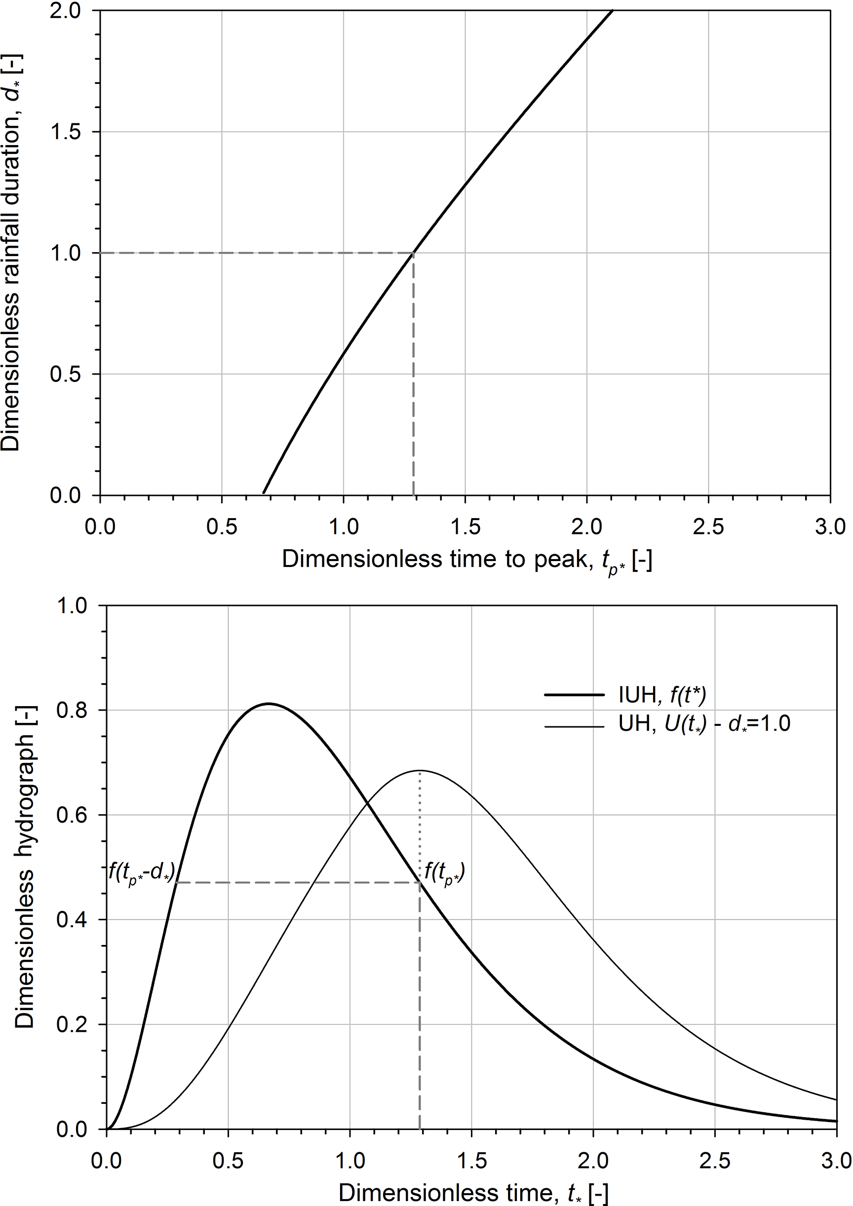
Figure 2 Dimensionless rainfall duration vs. dimensionless time to peak; dimensionless instantaneous unit hydrograph and the corresponding dimensionless unit hydrographs for $d_{\ast }=\mathrm{1}$.0. Note that the shape parameter α is equal to 3.

The dimensionless UH is evaluated, varying the dimensionless rainfall duration in the range between 0.5 and 2 in accordance with the n-structure definition in the range of durations [$d_i/\phantom{d_i\mathrm{2}}\mathrm{2};\mathrm{2}{d}_i$]; then the runoff peak analysis is carried out in the case of constant and variable runoff coefficients. The achieved results are presented with respect to the above-mentioned dimensionless duration range [0.5;2] that is wide enough to include the duration of the rainfall able to generate the maximum peak flow for a given catchment (Robinson and Sivapalan, 1997).

Finally the dimensionless procedure is applied to a small Mediterranean catchment. In the catchment application the dimensionless procedure is fully specified as from the evaluation of the rainfall structures associated with three observed rainfall events with regard to the determination of the reference peak flow and consequently of the dimensionless hydrograph peaks for the three observed rainfall structures.

3.1 Maximum dimensionless runoff peak with constant runoff coefficient

The dimensionless form of the hydrograph is shown in Fig. 3 with variation of the rainfall structure exponents, n, for the selected dimensionless rainfall duration. The hydrographs are obtained for excess rainfall intensities characterized by a constant runoff coefficient and rainfall structure exponents of 0.2, 0.3, 0.5 and 0.8.

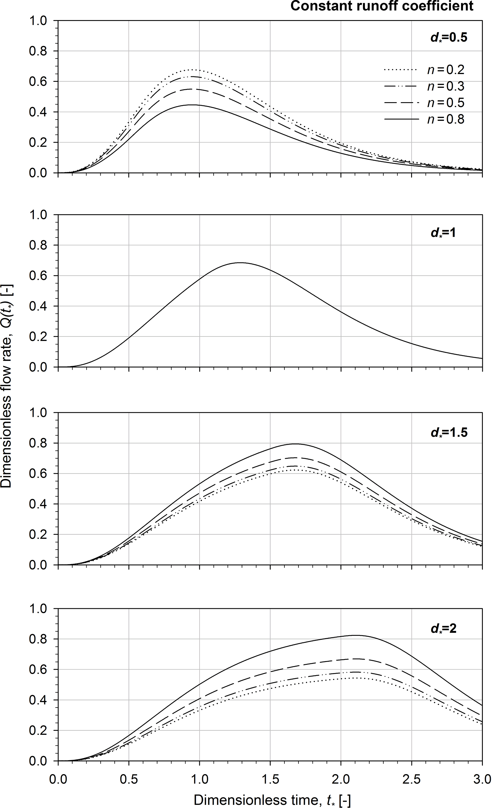
Figure 3 Dimensionless flow rates obtained for excess rainfall intensities characterized by constant runoff coefficient and different rainfall structure exponents, n (n= 0.2, 0.3, 0.5 and 0.8) at assigned dimensionless rainfall duration, d_∗ ($d_{\ast }=\mathrm{0}$.5, 1.0, 1.5 and 2.0). Note that the shape parameter α is equal to 3.

The impact of the rainfall structure exponents on the hydrograph form depends on the rainfall duration: for d_∗ lower than 1, the higher n the lower is the peak flow rate and vice versa. Figure 4 illustrates the 3-D mesh plot and the contour plot of the dimensionless runoff peak as a function of the rainfall structure exponent and the dimensionless rainfall duration. In the 3-D mesh plot as well as in the contour plot, it is possible to observe a saddle point located in the neighbourhood of d_∗ and n values equal to 1 and 0.3, respectively. Note that the intersection line (reported as bold line in Fig. 4) between the saddle surface and the plane of the principal curvatures where the saddle point is a minimum indicates the highest values of the runoff peak for a given n-structure exponent.

Figure 4 3-D mesh plot (a) and contour plot (b) of the dimensionless hydrograph peak as a function of the rainfall structure exponent and the dimensionless rainfall duration in the case of a constant runoff coefficient. The maximum dimensionless hydrograph peak curve is also reported (bold line).

Figure 5 Maximum dimensionless hydrograph peak and the corresponding rainfall structure exponent vs. dimensionless time to peak in the case of a constant runoff coefficient; dimensionless instantaneous unit hydrograph and the corresponding dimensionless unit hydrographs for $d_{\ast }=\mathrm{1}$.0. Note that the shape parameter α is equal to 3.

In Fig. 5, the maximum dimensionless hydrograph peak and the corresponding rainfall structure exponent are plotted vs. the dimensionless time to peak. Further, the dimensionless IUH and the corresponding dimensionless UH for $d_{\ast }=\mathrm{1}$.0 are reported as an example. The reference line (indicated as short–short–short dashed grey line in Fig. 5) illustrates the lower control line corresponding to the rainfall duration infinitesimally small. Note that the rainfall structure exponent that maximizes the runoff peak for a given duration can be simply derived as a function of the dimensionless time to peak (see Eq. 20). The maximum dimensionless hydrograph peak curve tends to one for long dimensionless rainfall duration ($d_{\ast }>\mathrm{3})$ when the corresponding n-structure exponent tends to one (see Eq. 18): for high values of n structure, the critical conditions occur for long durations that correspond to paroxysmal events for which the rainfall intensity remains fairly constant. The local minimum of the maximum dimensionless runoff peak curve (see Fig. 5) occurs at t_p∗ of 1.29 corresponding to n-structure value of 0.31 and d_∗ of 1, thus pointing out that the less critical runoff peak occurs at n-structure exponent values corresponding to those typically derived by the statistical analysis of the annual maximum rainfall depth series in the Mediterranean climate. Furthermore, it can be observed that different rainfall event conditions (i.e. rainfall structure exponent n and duration d_∗) in the neighbourhood of the local minimum point could determine comparable effects in term of the runoff peak value.

3.2 Maximum dimensionless runoff peak with variable runoff coefficient

The excess rainfall depth, in the case of variable runoff coefficient, is evaluated by assigning a value to the reference runoff coefficient. In particular, the reference runoff coefficient is defined as follows, utilizing Eq. (21):

$$\begin{array}{}\text{(28)}& {\mathit{\phi }}_{\mathrm{r}}={\displaystyle \frac{h_{\mathrm{r}}}{h_{\mathrm{r}}+S}}\to {\mathit{\phi }}_{\mathrm{r}}={\displaystyle \frac{\mathrm{1}}{\mathrm{1}+S_{\ast }}}.\end{array}$$

In order to provide an example of the proposed approach, the presented results are obtained assuming a dimensionless soil abstraction S_∗ of 0.25. It follows that the reference runoff coefficient φ_r is equal to 0.8.

Similarly to the results presented for the case of constant runoff coefficient, Fig. 6 illustrates the dimensionless hydrographs obtained for excess rainfall intensities characterized by variable runoff coefficient and n-structure exponents of 0.2, 0.3, 0.5 and 0.8 at assigned dimensionless rainfall duration ($d_{\ast }=\mathrm{0}$.5, 1.0, 1.5 and 2.0). The dimensionless hydrographs, obtained for the variable runoff coefficient, show the same behaviour as those derived for the constant runoff coefficient (see Figs. 3 and 6), even if they differ in magnitude, thus confirming the role of the variable runoff coefficient on the runoff peak. In particular, due to the variability of the infiltration process, the runoff peaks slightly decrease for rainfall duration lower than 1 (i.e. $d_{\ast }=\mathrm{0}$.5) when compared with those observed in the case of a constant runoff coefficient while they rise up for a duration larger than 1 (i.e. $d_{\ast }=\mathrm{1}$.5 and 2).

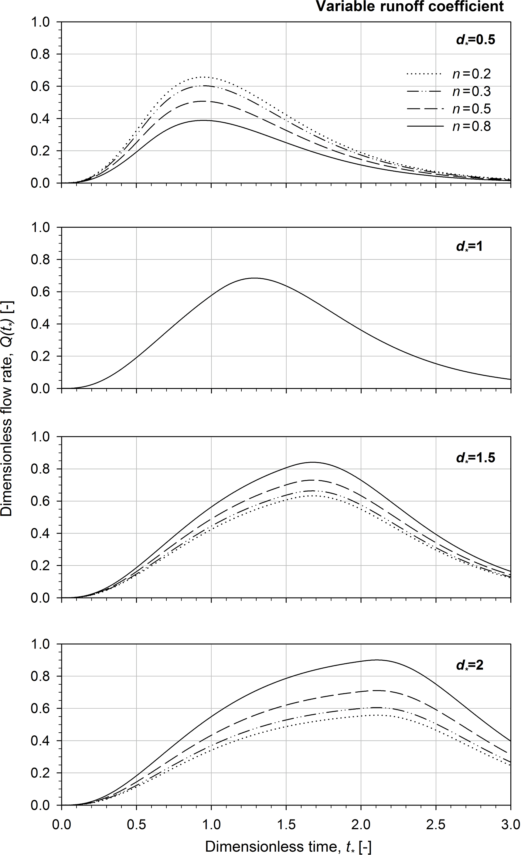
Figure 6 Dimensionless flow rates obtained for excess rainfall intensities characterized by a variable runoff coefficient and different rainfall structure exponents, n (n=0.2, 0.3, 0.5 and 0.8) at assigned dimensionless rainfall duration, d_∗ ($d_{\ast }=\mathrm{0}$.5, 1.0, 1.5 and 2.0). Note that the shape parameter α is equal to 3.

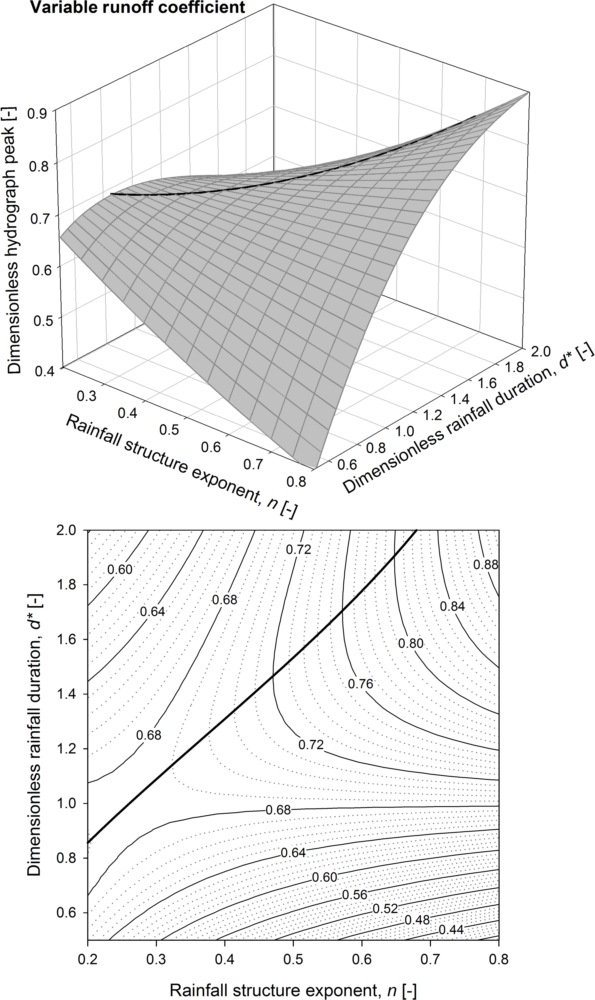
Figure 7 3-D mesh plot (a) and contour plot (b) of the dimensionless hydrograph peak as a function of the rainfall structure exponent and the dimensionless rainfall duration in the case of a variable runoff coefficient. The maximum dimensionless hydrograph peak curve is also reported (bold line).

Figure 7 shows the 3-D mesh plot and the contour plot of the dimensionless runoff peak as a function of the rainfall structure exponent and the dimensionless rainfall duration in the case of a variable runoff coefficient. By comparing Figs. 7 and 4, it emerges that the contour lines observed in the case of a variable runoff coefficient reveal a steeper trend with respect to constant runoff coefficient trends; indeed, the impact of the n-structure exponent on the hydrograph peak is enhanced when the runoff coefficient is assumed to be variable. The saddle point is again located in the neighbourhood of d_∗ and n values equal to 1 and 0.3, respectively, while the curve of the maximum values of the runoff peak (reported as bold line in Fig. 7) is moved to the left.

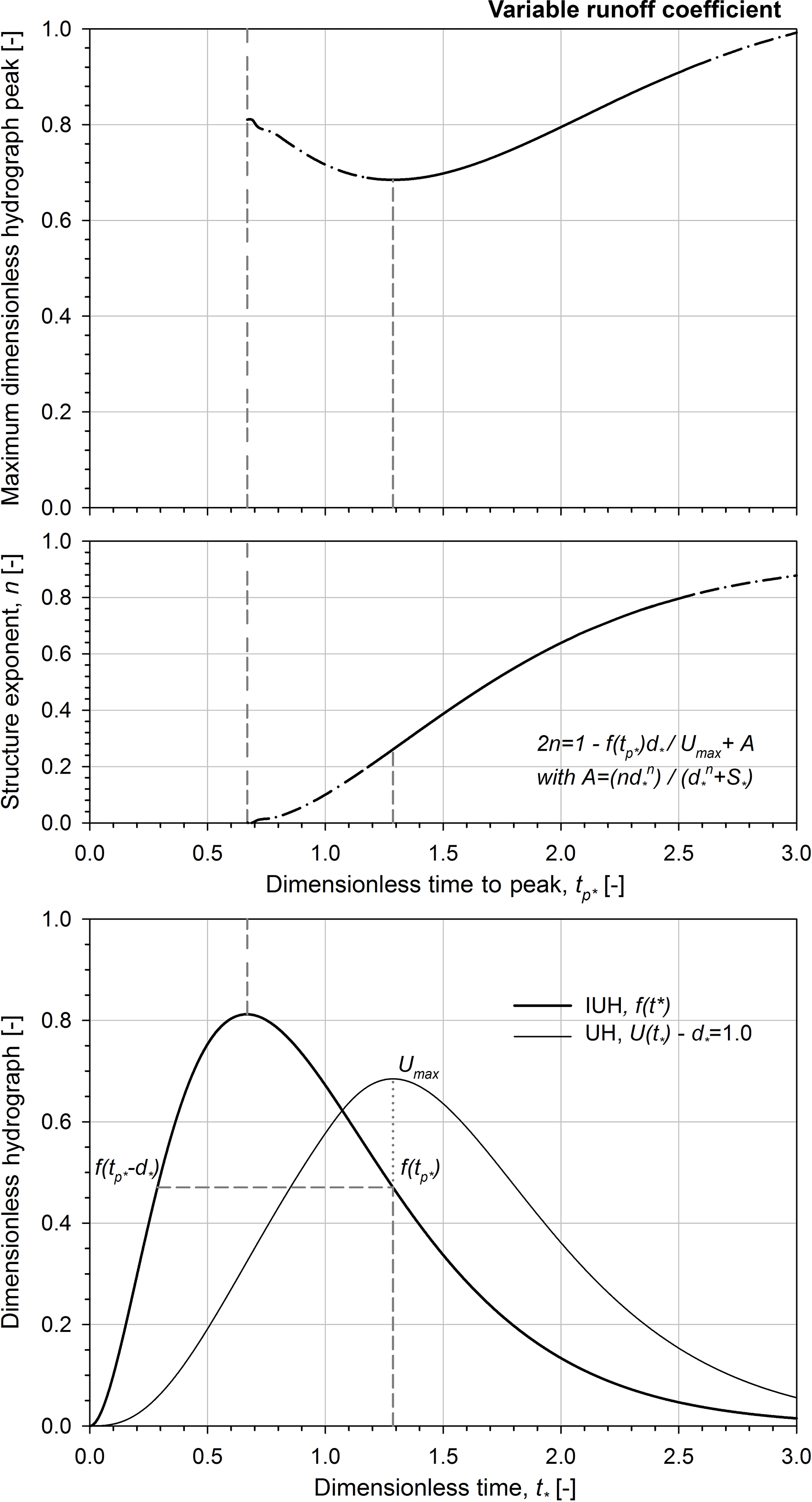
Figure 8 Maximum dimensionless hydrograph peak and the corresponding rainfall structure exponent vs. dimensionless time to peak in the case of a variable runoff coefficient; dimensionless instantaneous unit hydrograph and the corresponding dimensionless unit hydrographs for $d_{\ast }=\mathrm{1}$.0. Note that the shape parameter α is equal to 3.

In Fig. 8, the maximum dimensionless hydrograph peak and the corresponding rainfall structure exponent are plotted vs. the dimensionless time to peak in the case of a variable runoff coefficient. Results plotted in Fig. 8 confirm that the maximum runoff peak curve reveals the local minimum point at t_p∗ of 1.29, corresponding to n of 0.26 and d_∗ of 1. Referring to S_∗ of 0.25, the maximum dimensionless runoff peak tends to 1.25 for long dimensionless rainfall duration ($d_{\ast }>\mathrm{3})$ when consequently the n-structure exponent tends to 1 (see Eqs. 24 and 26). Figure 9 illustrates the influence of different variable runoff coefficients (i.e. for instance different initial moisture conditions or different soil characteristics) on the maximum dimensionless runoff peak. Similarly to Fig. 8, the maximum dimensionless hydrograph peak (see the top graph) and the corresponding rainfall structure exponent (see the centre graph) are plotted vs. the dimensionless time to peak in the case of a variable runoff coefficient (for S_∗ values of 0.25 and 0.67) together with the comparison to the case of constant runoff coefficient. The maximum dimensionless runoff peak is similar for short rainfall duration (i.e. t_p∗ lower than 1.5) when the variable runoff coefficient reduces the runoff component with respect to the reference runoff case (that is, also the constant runoff case i.e. $S_{\ast }=\mathrm{0}$). On the contrary, the maximum dimensionless runoff peak increases with increasing the dimensionless soil abstraction for long rainfall duration. Such behaviour is due to the rate of change in the runoff production with respect to the rainfall duration: with increasing the rainfall volume the relevance of runoff with respect to the soil abstraction rises. In other words, the n-structure exponent that maximizes the runoff peak decreases when the dimensionless soil abstractions are increased (see Eq. 27).

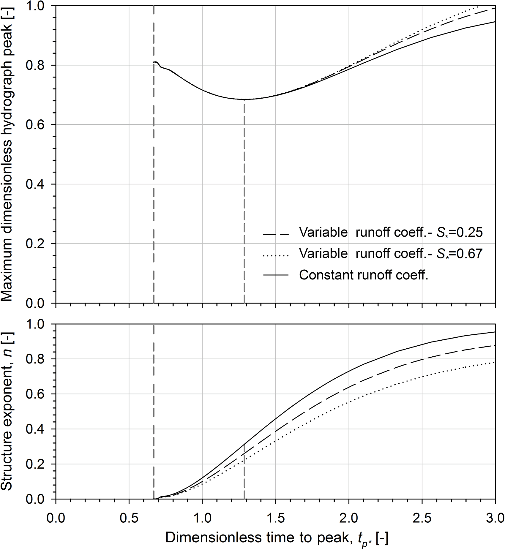
Figure 9 Maximum dimensionless hydrograph peak and the corresponding rainfall structure exponent vs. dimensionless time to peak in the case of variable runoff coefficients with respect to dimensionless maximum retention S_∗ of 0.25 and 0.67. The comparison to the case of constant runoff coefficient is also reported.

3.3 Catchment application

In order to point out the dimensionless procedure implications and to provide some numerical examples of the rainfall event structures, the proposed methodology has been implemented for the Bisagno catchment at La Presa station, located at the centre of Liguria region (Genoa, Italy).

The Bisagno–La Presa catchment has a drainage area of 34 km² with an index flood of about 95 m³ s⁻¹. The upstream river network is characterized by a main channel length of 8.36 km and mean streamflow velocity of 2.4 m s⁻¹. Regarding the geomorphology of the catchment, the area (R_A), bifurcation (R_B) and length (R_L) ratios that are evaluated according to the Horton–Strahler ordering scheme are respectively equal to 5.9, 5.6 and 2.5. By considering the altimetry, vegetation and limited anthropogenic exploitation of the territory, the Bisagno–La Presa is a mountain catchment characterized by an average slope of 33 %. The soil abstraction, S_II, is assumed to be equal to 41 mm; its evaluation is based on the land use analysis provided in the framework of the EU Project CORINE (EEA, 2009). The mean value of the annual maximum rainfall depth for unit duration (hourly) and the scaling exponent of the DDF curves are respectively equal to 41.31 mm h⁻¹ and 0.39. Detailed hydrologic characterization of the Bisagno catchment can be found elsewhere (Bocchiola and Rosso, 2009; Rulli and Rosso, 2002; Rosso and Rulli, 2002). With regard to the rainfall–runoff process, the two parameters of the gamma distribution are evaluated based on the Horton order ratio relationship (Rosso, 1984). The shape and scale parameters are estimated to be equal to 3.4 and 0.25 h respectively, thus corresponding to the lag time of 0.85 h.

In this application, three rainfall events observed in the catchment area have been selected in order to analyse the different runoff peaks that occurred for the three rainfall event structures. For comparison purposes, the selected events are characterized by an analogous magnitude of the maximum rainfall depth observed for the duration equal to the reference time (i.e. h_r=80 mm, t_r=0.85 h).

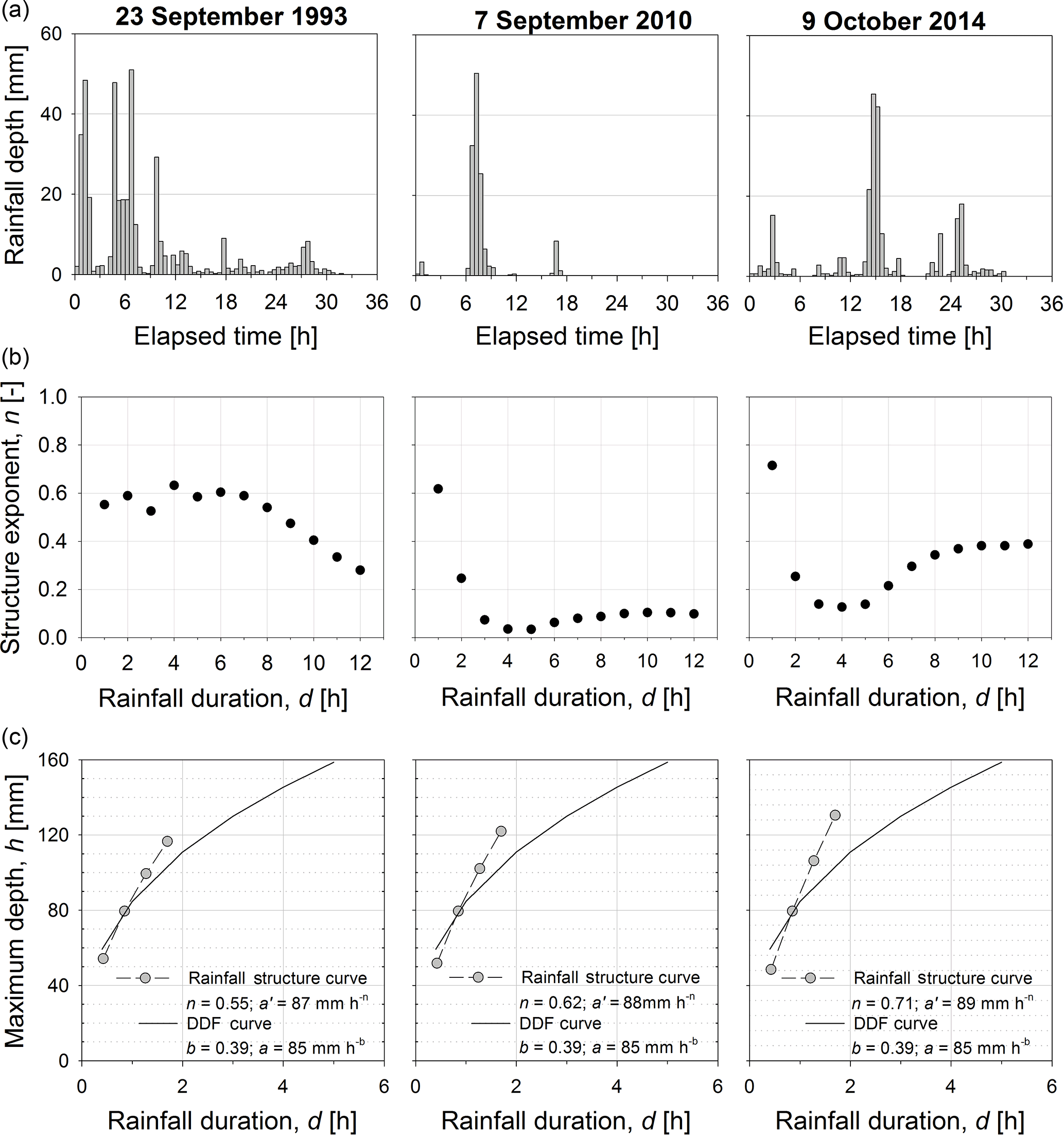
Figure 10 Rainfall event structure of three events observed in Genoa (Italy): the observed rainfall depths (a) and the estimated rainfall structure exponents (b) are reported. At the bottom, the rainfall structure and depth–duration–frequency curves, evaluated for the reference time of the Bisagno–La Presa catchment, are reported.

Figure 10 illustrates the rainfall event structure curves derived for the three selected rainfall events. The graphs at the top report the observed rainfall depths while the central graphs show the estimated rainfall structure exponents. At the bottom of Fig. 10, by considering the three structure exponents corresponding to the Bisagno–La Presa reference time (i.e. n=0.55, 0.62, 0.71), the rainfall event structure curves are derived for a rainfall durations ranging between 0.5⋅t_r and 2⋅t_r; for comparison purposes, the DDF curve is also reported. Based on each rainfall structure curve, four rectangular hyetographs with duration of 0.425, 0.85, 1.275 and 1.7 h in the range [$t_{\mathrm{r}}/\phantom{t_{\mathrm{r}}\mathrm{2}}\mathrm{2};\mathrm{2}{t}_{\mathrm{r}}$] are derived to evaluate the impact on the hydrograph peak of the Bisagno–La Presa catchment. Note that the analysis is performed in the case of a variable runoff coefficient whose reference value is equal to 0.66 (i.e. $S_{\ast }=\mathrm{0}$.5; S=41 mm). In Fig. 11, the excess rainfall hyetographs, the corresponding hydrographs and the reference value of the runoff peak flow are plotted for the three investigated rainfall structure exponents. The reference value of the runoff peak flow (dash–dot line) is evaluated by assuming a constant-intensity hyetograph of infinite duration and having excess rainfall intensity equal to that estimated for the reference time. The role of the rainfall structure exponent emerges in the different decreasing rate of the excess rainfall intensity with the duration, thus resulting in the corresponding increasing rate of the peak flow values.

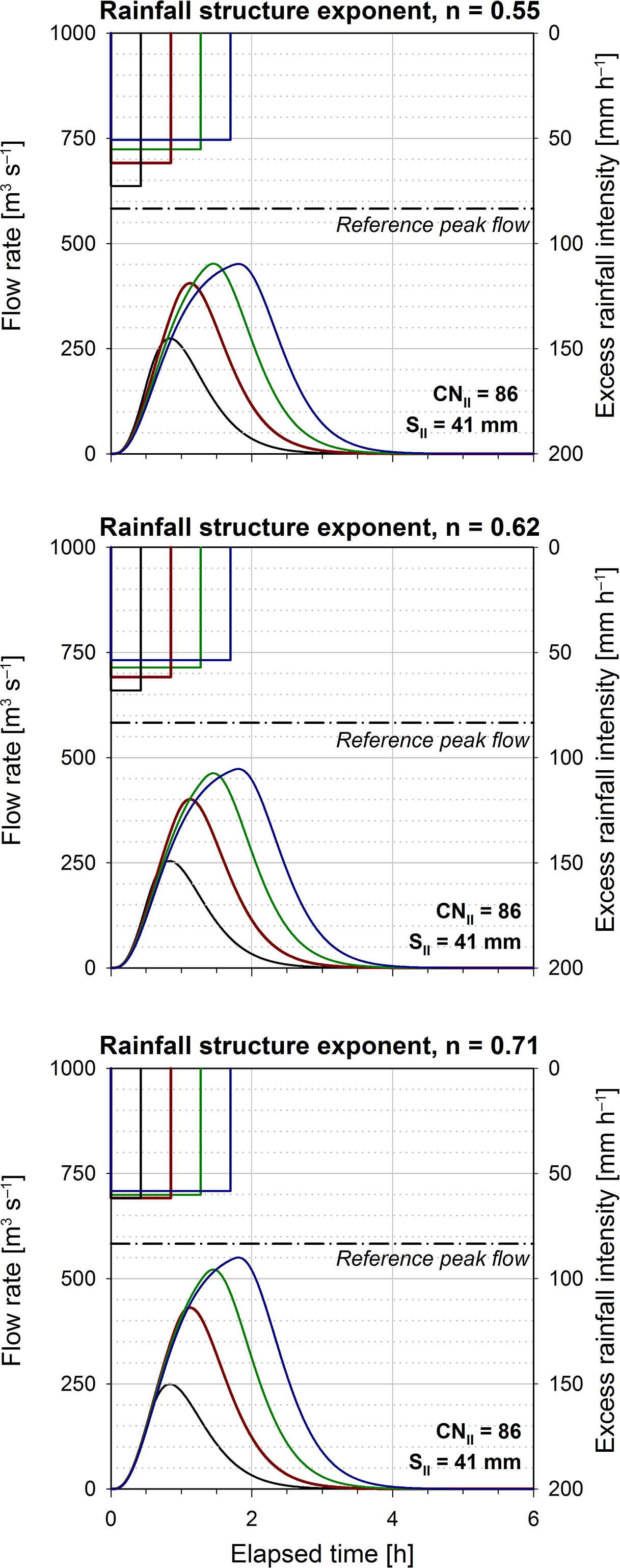
Figure 11 The excess rainfall hyetographs, the corresponding hydrographs and the reference value of the hydrograph peak flow evaluated for three rainfall structure exponents applied to the Bisagno–La Presa catchment. Note that each graph includes four rainfall durations (i.e. 0.5, 1.0, 1.5 and 2.0 times the reference time).

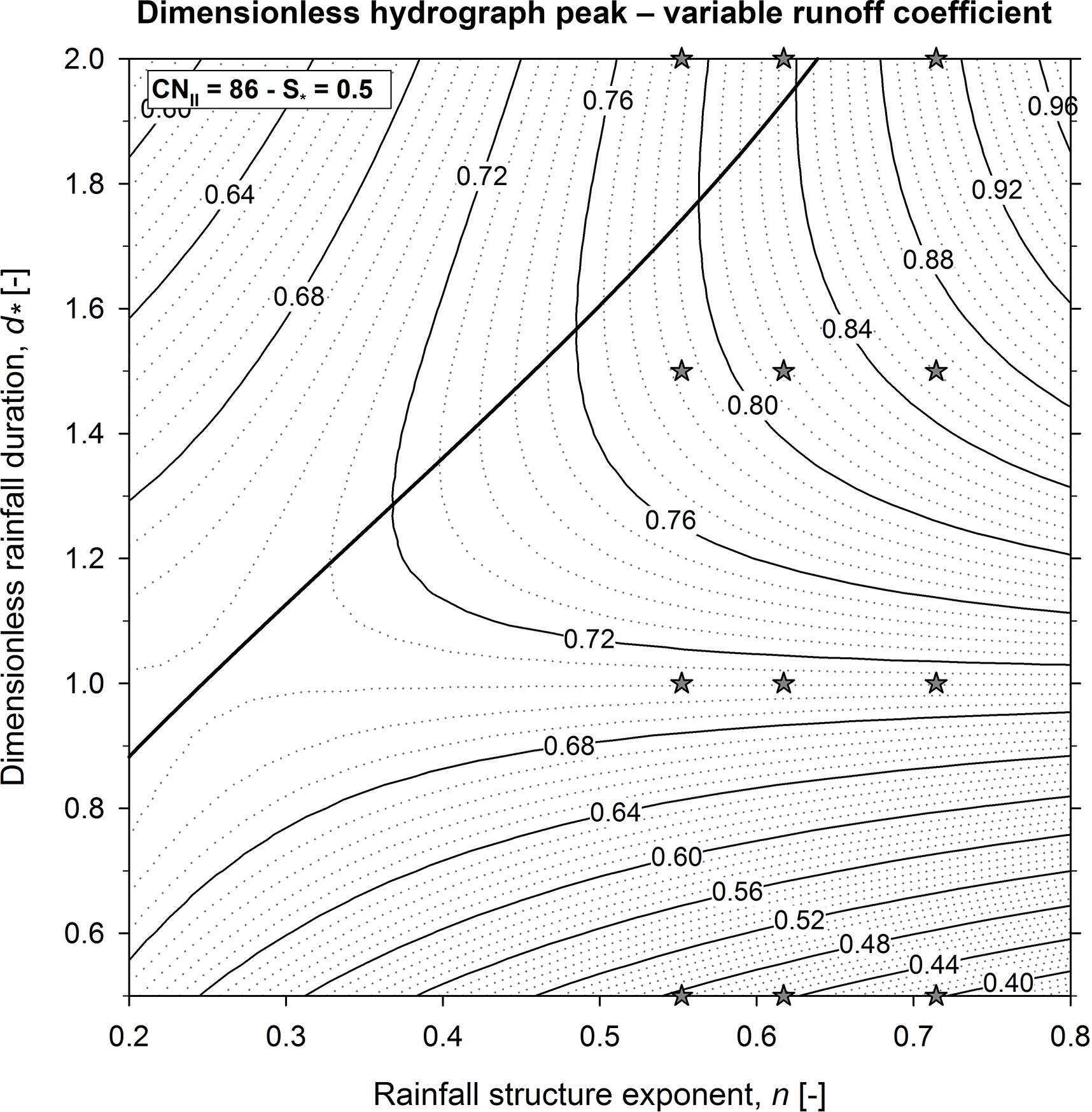
Figure 12 Contour plot of the dimensionless hydrograph peak evaluated for the Bisagno–La Presa catchment in the case of a variable runoff coefficient ($S_{\ast }=\mathrm{0}$.5). The maximum dimensionless runoff peak curve is also reported (bold line) together with the dimensionless hydrograph peaks (grey-filled stars) for the selected rainfall structure exponents (n=0.55, 0.62, 0.71) and durations ($d_{\ast }=\mathrm{0}$.5, 1.0, 1.5 and 2.0).

Figure 12 shows the contour plot of the dimensionless hydrograph peak in the case of a variable runoff coefficient ($S_{\ast }=\mathrm{0}$.5). The maximum runoff peak curve is also reported (bold line) together with the dimensionless hydrograph peaks (grey-filled stars) for the selected rainfall structure exponents (n=0.55, 0.62, 0.71) and durations ($d_{\ast }=\mathrm{0}$.5, 1.0, 1.5 and 2.0). Note that these selected rainfall structures represent only three of the possible outcomes in the sample space of the rainfall structures that are described in the contour plot. Similarly to Fig. 7, the Bisagno–La Presa catchment application shows a curve of the highest values of the runoff peak characterized by a local minimum (saddle point) in the neighbourhood of d_∗ and n values equal to 1 and 0.3, respectively.

4 Conclusions

The proposed analytical dimensionless approach allows the investigation of the impact of the rainfall event structure on the hydrograph peak. To this end a methodology to describe the rainfall event structure is proposed based on the similarity with the depth–duration–frequency curves. The rainfall input consists of a constant hyetograph where all the possible outcomes in the sample space of the rainfall structures can be condensed through the n-structure exponent. The rainfall–runoff processes are modelled using the Soil Conservation Service method for soil abstractions and the instantaneous unit hydrograph theory. In the present paper the two-parameter gamma distribution is adopted as an IUH form; however, the analysis can be repeated using other synthetic IUH forms obtaining similar results.

The proposed dimensionless approach allows an analytical framework to be defined which can be applied to any study case for which the model assumptions are valid; the site-specific characteristics (such as the morphologic and climatic characteristics of the catchment) are no more relevant, as they are included within the parameters of the dimensionless procedure (i.e. h_r(T_r) and t_r), thus allowing the implication on the hydrograph peak irrespective of the absolute value of the rainfall depth (i.e. the corresponding return period) to be figured out. A set of analytical expressions has been derived to provide the estimation of the maximum peak with respect to a given n-structure exponent. Results reveal the impact of the rainfall event structure on the runoff peak, thus pointing out the following features:

• The curve of the maximum values of the runoff peak reveals a local minimum point (saddle point).

• Different combinations of n-structure exponent and rainfall duration may determine similar conditions in terms of runoff peak.

• Analogous behaviour of the maximum dimensionless runoff peak curve is observed for different runoff coefficients although wider range of variations are observed with increasing soil abstraction values.

Referring to the Bisagno–La Presa catchment application (h_r=80 mm; t_r=0.85 h and $S_{\ast }=\mathrm{0}$.5), the saddle point of the runoff peaks is located in the neighbourhood of an n value equal to 0.3 and rainfall duration corresponding to the reference time ($d_{\ast }=\mathrm{1}$). Further, it emerges that the maximum runoff peak value, corresponding to the scaling exponent of the DDF curve, is comparable to the less critical value (saddle point). Findings of the present research suggest that further review is needed of the derived flood distribution approaches that coupled the information on precipitation via DDF curves and the catchment response based on the iso-frequency hypothesis. Future research with regard to the structure of the extreme rainfall event is needed; in particular the analysis of several rainfall data series belonging to a homogeneous climatic region is required in order to investigate the frequency distribution of specific rainfall structures.

The developed approach, besides suggesting remarkable issues for further researches and being unlike the merely analytical exercise, succeeds in highlighting once more the complexity in the assessment of the maximum runoff peak.