Estimating long-term groundwater storage and its controlling factors in Alberta, Canada

Groundwater is one of the most important natural resources for economic development and environmental sustainability. In this study, we estimated groundwater storage in 11 major river basins across Alberta, Canada, using a combination of remote sensing (Gravity Recovery and Climate Experiment, GRACE), in situ surface water data, and land surface modeling estimates (GWSA_sat). We applied separate calculations for unconfined and confined aquifers, for the first time, to represent their hydrogeological differences. Storage coefficients for the individual wells were incorporated to compute the monthly in situ groundwater storage (GWSA_obs). The GWSA_sat values from the two satellite-based products were compared with GWSA_obs estimates. The estimates of GWSA_sat were in good agreement with the GWSA_obs in terms of pattern and magnitude (e.g., RMSE ranged from 2 to 14 cm). While comparing GWSA_sat with GWSA_obs, most of the statistical analyses provide mixed responses; however the Hodrick–Prescott trend analysis clearly showed a better performance of the GRACE-mascon estimate. The results showed trends of GWSA_obs depletion in 5 of the 11 basins. Our results indicate that precipitation played an important role in influencing the GWSA_obs variation in 4 of the 11 basins studied. A combination of rainfall and snowmelt positively influences the GWSA_obs in six basins. Water budget analysis showed an availability of comparatively lower terrestrial water in 9 of the 11 basins in the study period. Historical groundwater recharge estimates indicate a reduction of groundwater recharge in eight basins during 1960–2009. The output of this study could be used to develop sustainable water withdrawal strategies in Alberta, Canada.

1 Introduction

Fresh water is an important resource for economic development and social sustainability around the world. Approximately 1.2 billion people live in water-scarce areas across the globe (UN-Water/FAO, 2007). More than a billion people lack access to safe drinking water and this number is increasing due to an increasing population (Connor, 2015). However, the effects of climate change on glaciers and snowpack and the effects of human activities, such as overuse and overextraction of resources, can result in lowering water tables and groundwater depletion (Scanlon et al., 2016; Bhanja et al., 2017b). In situ monitoring of wells is the traditional approach for estimating groundwater storage. However, well monitoring is spatially not continuous and has a high cost for a large region. There are only scant observation stations in some areas, especially in semiarid and arid environments, or cold climate regions covered by glacier and snowpack, due to difficulties of access and monitoring. As a result, proper groundwater management and decision-making are hampered considerably by the scarcity of data.

Remote-sensing data from the Gravity Recovery and Climate Experiment (GRACE) satellite mission could be used to estimate groundwater storage at a continuous and large scale across the globe and offer a new opportunity for groundwater storage assessment (Rodell et al., 2007). Although the GRACE satellite mission currently provides global-scale data for the detection of temporal gravity changes (Tapley et al., 2004), these temporal gravity changes are not a direct measurement of groundwater storage. A relationship would have to be established between temporal gravity changes and groundwater storage variations through the continuously evolving algorithms (Watkins et al., 2015). Estimates of groundwater storage using the remote sensing have been performed around the globe (Swenson et al., 2006; Rodell et al., 2007, 2009; Strassberg et al., 2007; Tiwari et al., 2009; Scanlon et al., 2012; Shamsudduha et al., 2012; Voss et al., 2013; Bhanja et al., 2014, 2016, 2017b, 2018; Richey et al., 2015; Panda and Wahr, 2016; Chen et al., 2016; Long et al., 2016). Huang et al. (2016) used remote-sensing data for computing the groundwater storage anomalies (GWSAs) in order to estimate groundwater storage in Alberta. They used groundwater levels (GWLs) at 36 wells, mostly confined to the southern Alberta region, and were correlated with both the GRACE terrestrial water storage (TWS) and groundwater storage variations. Then they compared the TWS with GWLs instead of the groundwater storage and without considering surface water data due to the lack of available high-resolution data.

Recent studies (e.g., Huang et al., 2015; Nanteza et al., 2016) have considered both confined and unconfined aquifers for in situ GWSA computation but they have not separated the data from the two types. The two types of aquifers have different recharge and storage patterns. Confined aquifers are overlain by relatively impermeable rock or clay, which limits vertical water infiltration, while in unconfined aquifers, vertical water infiltration can occur from precipitation, snowmelt, surface water, etc. The two types of aquifers also respond differently to effects from pumping (Alley et al., 1999). Therefore, these should be studied separately for estimating groundwater storage in a region. Further, Rodell et al. (2007) indicated the importance of surface water factors in the GWSA estimation and sought for inclusion of surface water storage variations in GWSA disaggregation. They also pointed out the importance of separating contributions by temporal mass variability using auxiliary observations and numerical models when estimating groundwater storage changes in large-scale regions. In cold climate regions, such as in Alberta, the surface water could make a significant contribution to groundwater storage variations due to the effects of climate change on snowpack, glaciers, permafrost, and wetlands. Therefore, more efforts are required to properly evaluate groundwater storage for aquifer storage coefficients in transforming GWL information to groundwater storage in cold climate regions (Feng et al., 2013). The main objectives of this study are

1. to investigate the long-term groundwater storage conditions in cold climate regions, such as the 11 river basins in Alberta, Canada, by combining all of the processing steps, such as the surface water storage estimates.

2. to validate the remote-sensing estimates from two different remote-sensing products using the maximum available in situ observation well data; the in situ groundwater storage has been estimated by combining the storage coefficients and aquifer thickness (for confined aquifers) with the water table fluctuation.

3. to find the role of natural hydrological components (e.g., precipitation, snowmelt, evapotranspiration) in influencing groundwater storage variations; we have also studied long-term groundwater recharge trends from a global-scale hydrological model for inferring long-term variabilities in groundwater recharge rates.

Table 1 Details of the river basins used (within Alberta only), number of wells used, precipitation, and GWSA_obs trends (statistically significant (p value < 0.01) trend estimates are shown in bold).

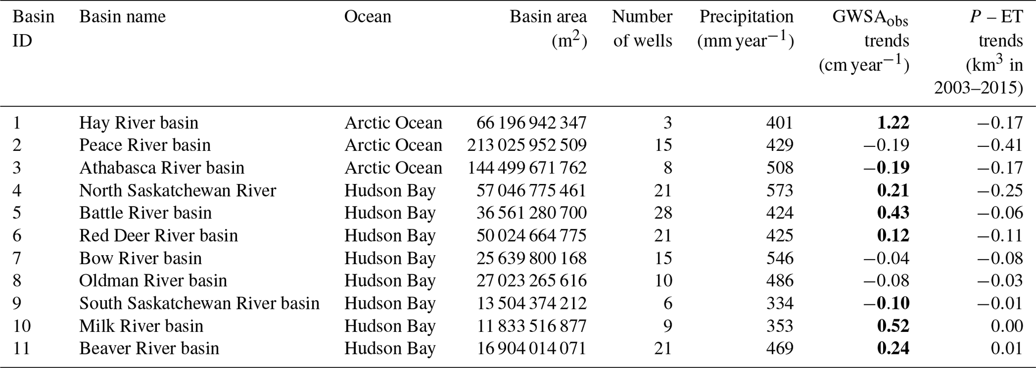
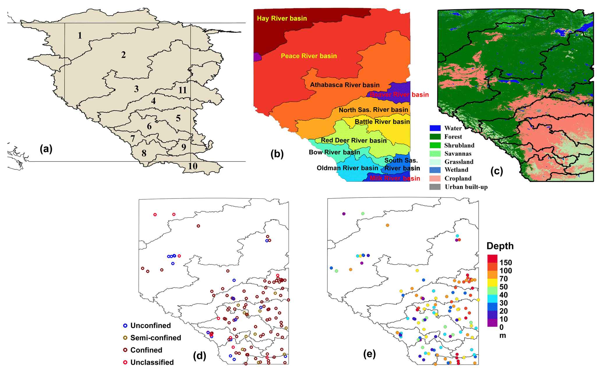
Figure 1 Major river basins in Alberta. (a) Full basin extent; (b) Alberta only; (c) dominant land cover types; (d) aquifer types represented through the studied wells; (e) depth of wells screened in Alberta, overlaid by basin boundaries.

Figure 2 Annual precipitation rates (mm year⁻¹) in Alberta between 2003 and 2014.

2 Materials and methods

2.1 Study area

This study has been conducted in the major river basins (the map has been made following Lemay and Guha, 2009; AEP, 2011; AEP, 2017) within the province of Alberta (Fig. 1a, b). The Peace River basin is the largest basin in the province, followed by the Athabasca River basin and Hay River basin (Table 1). Most parts of the study region have been characterized as cold climate regions (Peel et al., 2007). Basin-scale annual average precipitation varies within 330 to 570 mm year⁻¹ (Table 1). We used Global Land Cover Facility (GLCF) native-resolution data (resolution: ∼460 m × 460 m; http://www.landcover.org/, last access: 2 October 2017) for characterizing land cover (Channan et al., 2014). Most of the land areas in Alberta are covered by natural vegetation (i.e., forest, shrubland, mixture of shrub and grassland, and grassland; Fig. 1c, Table S1 in the Supplement). The second most prevalent land-cover type is cropland (Fig. 1c, Table S1). Surface water bodies (water and permanent wetland) cover less than 6 % of the area of all the river basins (Fig. 1c, Table S1).

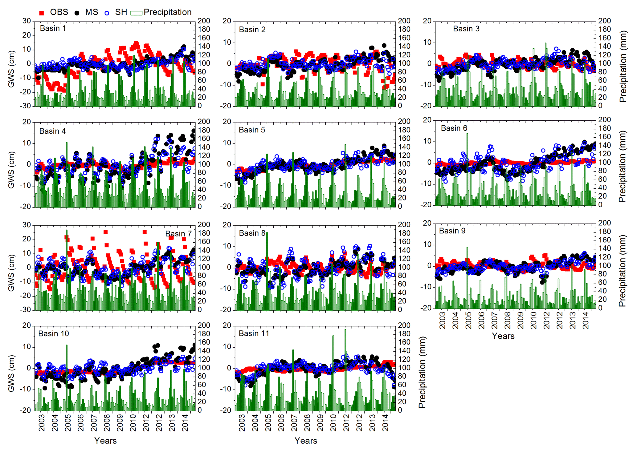
Figure 3 Basin-wide, monthly time series of in situ GWSA (OBS, red squares) and GWSA obtained using the GRACE mascon product (MS, black filled circles) and GRACE SH products (SH, blue open circles). Monthly spatially averaged precipitation data are shown using green columns.

We used monthly mean precipitation data from the archives of the Climatic Research Unit (CRU), University of East Anglia. The quality-controlled, gridded $\mathrm{0.25}{}^{\circ }\times \mathrm{0.25}{}^{\circ }$, monthly mean TS4.0 total precipitation products are used here (Harris et al., 2014). The precipitation-gauge-based data were collected through the World Meteorological Organization (WMO), National Oceanographic and Atmospheric Administration (NOAA), and other international and national agencies across the globe for preparing this dataset (Harris et al., 2014). The precipitation data are spatially averaged in order to provide basin-scale data. CRU data have been found to have the best match of other available products while comparing with in situ precipitation measurements in China (Zhao and Fu, 2006). Precipitation data exhibit temporal as well as spatial variations in the study period with values of 150 to >1000 mm year⁻¹ (Fig. 2). In general, the lowest precipitation was observed in 2004 and the highest in 2010 (Fig. 2). Spatially averaged basin-scale precipitation values indicate the highest precipitation rates prevail in the North Saskatchewan River basin (basin 4, 573 mm year⁻¹; Table 1) and the lowest rates prevail in the South Saskatchewan River basin (basin 9, 334 mm year⁻¹; Table 1). Precipitation rates are highly seasonal in Alberta (Fig. 3).

2.2 In situ measurements of groundwater storage

GWL depth data are obtained from the Alberta Environment and Parks, Government of Alberta (http://environment.alberta.ca/apps/GOWN/#, last access: 14 September 2017). Daily GWL depth data are obtained for 470 monitoring wells distributed across the province of Alberta. The data are screened for data continuity (at least 80 % of the data are present in each location) within the study period of 2003–2015, resulting in the use of GWL data from 157 measurement locations. Daily GWL information is converted to monthly GWL at individual locations. Because of the differences in groundwater storage variations within different types of aquifers, these wells need to be classified as unconfined, semi-confined, and confined. Out of the 157 measurement locations used in the study, 24 are located in unconfined aquifers, 17 are located within semi-confined aquifers, 100 are located within confined aquifers, and 16 are unclassified (Fig. 1d). Basin-wide details of the distribution of wells are provided in Table S2. The screen depth of the wells varies from 6 to 220 m (Fig. 1e). The wells located in unclassified or semi-confined aquifers are characterized as either confined or unconfined based on their location hydrogeology and screen depth. For example, a well screened at a semi-confined aquifer with shallower depth and underlain by permeable materials can be classified as an unconfined aquifer for storage calculations and vice versa.

We have studied the subsurface hydrogeology in detail using well-specific lithology information from the Alberta Environment and Parks, Government of Alberta (http://environment.alberta.ca/apps/GOWN/#, last access: 14 September 2017). In order to compute groundwater storage anomalies (GWSA_obs) in an unconfined aquifer, the GWSA needs to be accurately represented using the storage coefficients of the aquifer (Scanlon et al., 2012). We have followed the equation (Todd and Mays, 2005; Bhanja et al., 2017a)

$$\begin{array}{}\text{(1)}& {\mathrm{GWSA}}_{\mathrm{obs}}=(h_m\times S_{\mathrm{y}}-h_i\times S_{\mathrm{y}}),\end{array}$$

where h_m and h_i represent the mean GWL depth and GWL depths at different time periods at a location; S_y represents the specific yield of the aquifer. S_y is assigned to the individual data based on the specific yield of the geologic material in its screen position. Specific yield data corresponding to a specific geologic material are presented in Table S3.

GWSA_obs values in a confined aquifer have been estimated following the equation (Todd and Mays, 2005)

$$\begin{array}{}\text{(2)}& {\mathrm{GWSA}}_{\mathrm{obs}}=(h_m\times S_{\mathrm{s}}\times b-h_i\times S_{\mathrm{s}}\times b),\end{array}$$

where S_s is the specific storage and b is the thickness of the aquifer. S_s of a material varies over a wide range; the details of material-specific S_s are provided in Table S4. Thickness of the aquifer for the individual aquifer units is obtained from the Alberta Environment and Parks, Government of Alberta. The data are assigned to individual wells based on their screening zone and thickness of the particular aquifer unit.

2.3 Surface water storage processing

Surface water level daily time series are obtained (n=393) from the Water Office, Government of Canada (https://wateroffice.ec.gc.ca/, last access: 25 August 2017) for the study region. After rearranging the data based on near-continuous data availability, we used 65 locations with >80 % of the data availability range. The data are temporally averaged at each location for estimating monthly mean values. The number of locations that fall within each of the river basins are spatially averaged to obtain the month-scale spatially averaged surface water anomaly. The surface water coverage fraction varies over the study region (Fig. 1c and Table S1). In order to obtain realistic surface water storage variations, surface water area fractions have been multiplied with the spatially averaged surface water anomaly in each river basin.

Figure 4 Basin-wide estimates of (a) RMSE, (b) correlation, (c) skewness, and (d) kurtosis.

Figure 5 Basin-wide coefficient of variation (CV) analysis for in situ GWSA (OBS, red squares) and GWSA obtained using the GRACE mascon product (MS, black filled circles) and GRACE SH products (SH, blue open circles).

2.4 Gravity Recovery and Climate Experiment (GRACE)

We have obtained the monthly mean liquid water equivalent thickness $\mathrm{1}{}^{\circ }\times \mathrm{1}{}^{\circ }$ gridded data from the archives of the National Aeronautics and Space Administration (NASA) Jet Propulsion Laboratory (JPL). JPL mascon solutions, version RL05, was used for 137 months (the data were not available for some of the months; details can be found in Watkins et al., 2015) between January 2003 and April 2015. The GRACE mission observes changes in gravity in the Earth's subsurface and provides the data on a continuous basis. The gravity change information has been processed further in order to obtain the TWS change data (details can be found here: http://grace.jpl.nasa.gov/data/get-data/jpl_global_mascons/, last access: 14 November 2017). Satellite laser ranging (SLR) has been incorporated for estimating degree 2 and order 0 coefficients (Cheng and Tapley, 2004). Processes to improve the geocenter correction have been reported by Swenson et al. (2008). The post-glacial rebound signals related to glacial isostatic adjustment (GIA) are removed using the process by Geruo et al. (2013). In the mascon approach, the entire globe is characterized as equally spaced 3^∘ spherical mass concentration blocks (Watkins et al., 2015). In order to improve the TWS estimates, scale factors provided with the data are multiplied (Bhanja et al., 2016). Scale factors are estimated in order to improve the performance of the TWS estimates.

The TWS information related to spherical harmonics (SH) has been obtained for 137 months (between January 2003 and April 2015) from the NASA JPL archive. We used $\mathrm{1}{}^{\circ }\times \mathrm{1}{}^{\circ }$ gridded RL05 datasets of SH solutions (Landerer and Swenson, 2012). Three independent solutions from the Center for Space Research at the University of Texas at Austin, the NASA JPL, and the German Space Agency (GFZ) were retrieved and combined to use in this study. Like the mascon approach, several similar techniques are applied to obtain the TWS change in the SH approach (source: http://grace.jpl.nasa.gov/data/get-data/monthly-mass-grids-land/, last access: 14 November 2017). Errors associated with N–S stripes in the TWS data are removed using a de-striping filter. A Gaussian filter of 300 km in width is also applied to the data. In order to improve the TWS estimates, the scale factors provided with the data are multiplied (Bhanja et al., 2016).

One advantage of the mascon approach is the introduction of a priori information that leads to the removal of correlated noise (stripes) in the data. As a result, post-processing filters are not required to be applied (Watkins et al., 2015). TWS data obtained from the mascon approach are less dependent on scale factors for estimating basin-scale mass change estimates (Watkins et al., 2015).

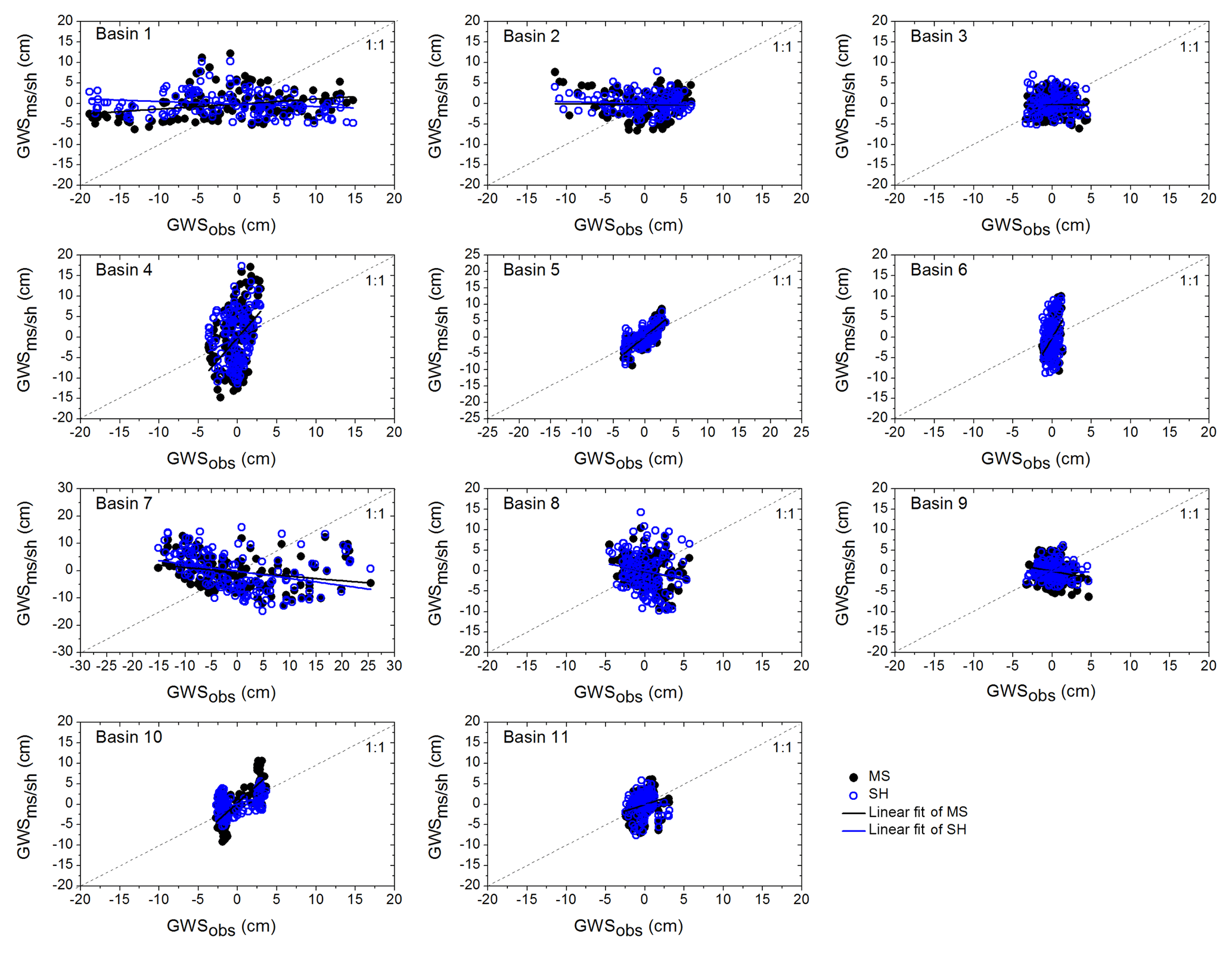
Figure 6 Basin-wide scatter analysis of in situ GWSA with the GWSA obtained using the GRACE mascon product (MS, black filled circles) and GRACE SH products (SH, blue open circles).

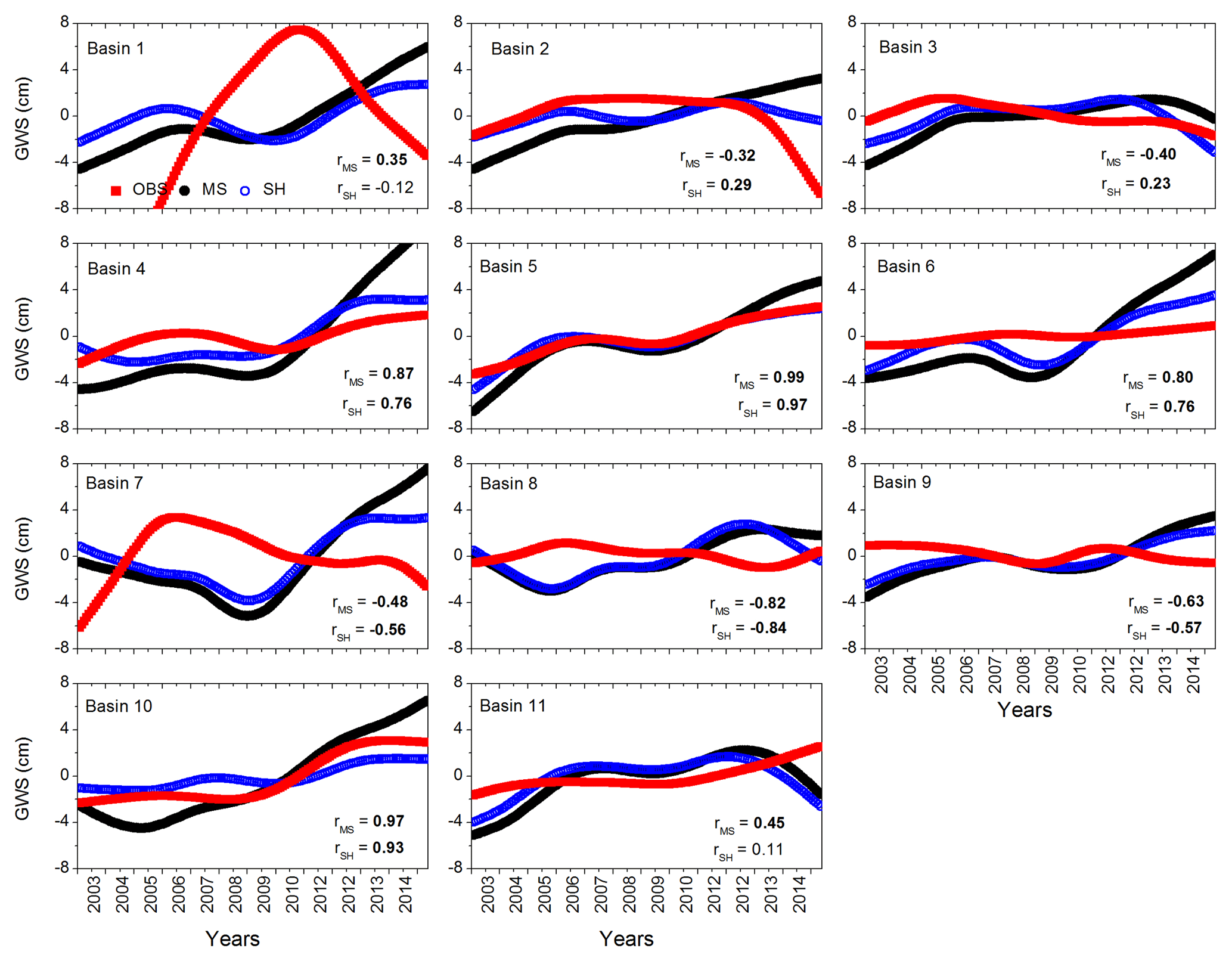
Figure 7 Basin-wide time series of HP filter data for in situ GWSA (OBS, red squares) and GWSA obtained using the GRACE mascon product (MS, black filled circles) and GRACE SH products (SH, blue open circles). Pearson's correlation coefficient values are provided in the inset and statistically significant (p value < 0.01) values are shown in bold.

2.5 Estimating groundwater storage from remote sensing and global models

Satellite-based groundwater storage anomalies (GWSA_sat) are estimated using a mass balance approach after removing other components of the hydrological cycle from the TWSA. These components include soil moisture anomaly (SMA), anomalies in snow water equivalents (SNAs), and anomalies in surface water variations (SWAs). Anomalies are estimated after removing the all-time mean value from the individual monthly values for all of the components. Soil moisture and snow water equivalent data were retrieved from NASA's Global Land Data Assimilation System (GLDAS) (Rodell et al., 2004) for 148 months in the study period. The GLDAS includes observation data from satellite sensors and ground-based measurements in order to improve the simulation output (Rodell et al., 2015). Bhanja et al. (2016) reported better GWSA estimates while using a combination of data from simulations of three different land surface models (LSMs), comparing the use of any single model's output. We also used a combined estimate from the outputs of the Community Land Model (CLM), Variable Infiltration Capacity (VIC), and Noah (Rodell et al., 2004). Surface water variation plays an important role in estimating GWSA. We have computed the surface water variations using in situ data, described in Sect. 2.3. GWSA can be estimated using the following equation:

$$\begin{array}{}\text{(3)}& {\mathrm{GWSA}}_{\mathrm{sat}}=\mathrm{TWSA}-\mathrm{SMA}-\mathrm{SNA}-\mathrm{SWA}.\end{array}$$

2.6 Groundwater recharge from global-scale hydrological model

In order to find the historical groundwater recharge pattern, we used a global-scale hydrological model, WaterGAP (version 2.2) (Doll et al., 2014) to estimate long-term groundwater recharge data (1960–2009). The WaterGAP simulates global-scale water storage and transport including human water use and groundwater recharge from surface water bodies at $\mathrm{0.5}{}^{\circ }\times \mathrm{0.5}{}^{\circ }$ resolution (Doll et al., 2014). Water withdrawal from both groundwater and surface water has also been considered. We used a combination of diffuse groundwater recharge and recharge from the surface water bodies, which we termed “total groundwater recharge”. As the WaterGAP simulation considers a simple water balance approach for groundwater recharge estimation, uncertainties may arise as a function of groundwater table gradient (Doll et al., 2014). Furthermore, increasing groundwater recharge from surface water bodies as a function of groundwater withdrawal has not been considered here (Doll et al., 2014). More information on model processes, data used, and other details can be found in Doll et al. (2014).

2.7 Statistical approaches

In order to compare the datasets using statistically robust techniques, we have used the root-mean-square error (RMSE), Pearson's correlation, skewness, kurtosis, and the coefficient of variation. RMSE has been used to show the departures from the true (in situ estimates here) value (Helsel and Hirsch, 2002). The trend analyses are based on the linear regression analysis. In order to represent the nonlinearity present within the data, we used the Hodrick–Prescott (HP) filter (Hodrick and Prescott, 1997), a nonparametric, nonlinear trend analysis. The HP filter employs a specific approach for separating trend (T_t) and cycle (c_t) components in the data (y_t).

$$\begin{array}{}\text{(4)}& y_t=T_t+c_t\end{array}$$

In order to estimate the trend and cycle separately, the HP filter solves the following equation (Hodrick and Prescott, 1997):

$$\begin{array}{}\text{(5)}& \mathrm{Min}\left(T\right){\sum }_{t=\mathrm{1}}^T({\left(y_t-T_t\right)}^{\mathrm{2}}+(\left(T_{t+\mathrm{1}}-T_t\right)-\left(T_t-T_{t-\mathrm{1}}\right){)}^{\mathrm{2}},\end{array}$$

where T_t+1 and T_t−1 represent the trend component with time steps of t+1 and t−1, respectively. The long-term average of the cyclical components is close to zero (Hodrick and Prescott, 1997). The smoothing parameter (λ) is a positive number that reduces the variability within cyclical components (Hodrick and Prescott, 1997). The value of λ was chosen to be 14 400 for monthly data (Hodrick and Prescott, 1997; Ravn and Uhlig, 2002).

Figure 8 Basin-wide time series of HP filter data for in situ GWSA (OBS, red squares), precipitation data (green circles), and rainfall + snowmelt data (blue circles). Pearson's correlation coefficient (r) values are provided in the inset and statistically significant (p value < 0.01) values are shown in bold. r_p and r_rs indicate the correlation between GWSA and precipitation and between GWSA and rainfall + snowmelt, respectively.

2.8 Assumptions and limitations

On the basis of data availability, we have not included the entire extent of the river basins (Fig. 1a) in the current analysis. The river basins are selected based only on their geopolitical extent in the province of Alberta (Fig. 1b). For in situ estimates, GWSA information is spatially averaged for providing the basin's GWSA estimates and also to compare them with the satellite-based estimates following Bhanja et al. (2017a) and Scanlon et al. (2018). The time period of the study is restricted by the availability of data. Separation of GWSA signals from TWSA by removing all other components is a challenging task due to the lack of in situ measurements of other components and the large uncertainties associated with LSM-simulated products (Scanlon et al., 2015). We have shown the satellite-based estimates for all of the basins; however, users should be cautious to use GRACE data in the smallest basins. This is because GRACE's native resolution could not allow users to directly use the data for smaller basins. Other processes such as the use of GRACE and integrated land surface model's operation could make the data available to use for smaller basins (Landerer and Swenson, 2012; Watkins et al., 2015). Data processing methods proposed by Dutt Vishwakarma et al. (2016) could be used to make the data available for smaller basins with GRACE SH products.

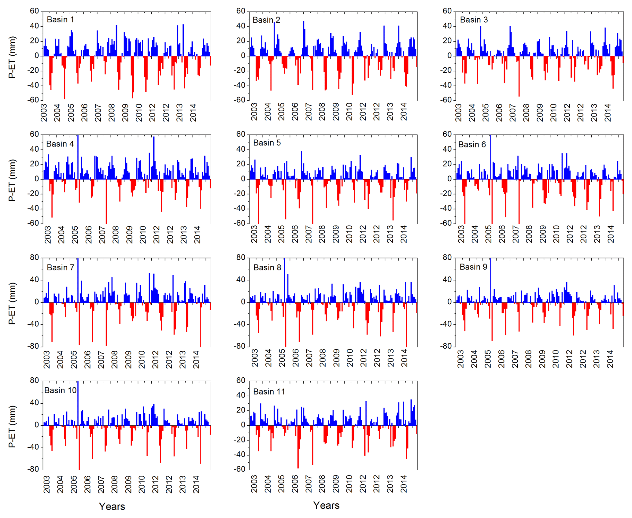
Figure 9 Basin-wide time series of P – ET values. Positive values are shown in blue and negative values are shown in red.

3 Results and discussions

3.1 Groundwater storage anomalies

In situ GWSA (GWSA_obs) values ranged from −30 to 30 cm in all of the basins, with the highest fluctuations observed in basin 7. GWSA_obs exhibits near zero values in basins 5, 6, 10, and 11 (Fig. 3). GWSA_obs magnitudes in different basins can arise as a result of diversity in specific yield values in the underlying material (Table S3). In situ estimates show seasonality, i.e., variations with precipitation rates, in basin 7. Trends in the GWSA_obs show decreasing GWSA between 2003 and 2015 in basins 2, 3, 7, 8, and 9 (Table 1). The results indicate that GWSA_obs depletion is in the range of −0.20 in basins 2 and 3. It is interesting to note that basins 7, 8, and 9 are composed of >25 % cropland (Table S1). Basin 3 has been subjected to the highest amount of licensed groundwater withdrawal allocation in Alberta (basin 3 accounts for 39 % of the total groundwater usage in Alberta). Conversely, an increasing trend has been observed in the remaining basins (Table 1). One probable cause for the groundwater table increase in these basins could be related to precipitation variability. The study region has been subjected to large-scale drought during 1999–2005 (Hanesiak et al., 2011). As a result, the TWS recovery in 2004–2007 has also been observed by Lambert et al. (2013).

Another important factor influencing groundwater recharge as well as the groundwater storage is the snowmelt processes prevailing in cold regions during the onset of spring–summer. The river basins have been receiving a substantial amount of snowfall during winter months (Fig. 3). This leads to snow accumulation in the region. At the end of the winter season, snowmelt processes majorly account for our observation of increasing GWSA in April onwards (Fig. 3). The observation is in line with the observations from the earlier studies conducted within the study region (Hayashi and Farrow, 2014; Hood and Hayashi, 2015). Comparatively higher rates of precipitation during summer months and the snowmelt during the start of the summer season are the major processes responsible for the observation of higher GWSA during summertime in the entire study region (Fig. 3).

GWSA_obs values from the unconfined aquifers reflect a higher magnitude than those in the confined aquifers (Fig. S1). This is because of the intrinsic property of the different types of aquifers. For instance, de-watering from the saturated zone during a pumping event is mainly responsible for the release of water in an unconfined aquifer (Alley et al., 1999). Conversely, a net decrease in groundwater potential and associated reduction in water pressure have occurred during a pumping event in a confined aquifer. The indigenous water expands slightly due to the decrease in water pressure, leading to slight compression in the aquifer material (Alley et al., 1999). This can explain why the groundwater storage change in the confined aquifers is comparatively lower than that in the unconfined aquifers.

Remote-sensing estimates of GWSA (GWSA_sat) using the two different assessments, GRACE MS and GRACE SH approaches, show temporal variations ranging from −20 to 20 cm. However, the seasonal amplitudes are not similar in different basins (Fig. 3). In general, the magnitude of the GWSA_sat compares well with that of the GWSA_obs (Fig. 3). GWSA_sat exhibits large amplitudes in basins 4, 7, and 8 (Fig. 3). In general, the GWSA_sat estimates from the two products match well with the observed estimates (Fig. 3). The estimations are in line with the values reported for the Mackenzie River basin by Scanlon et al. (2018). Overall, the two satellite-based estimates are found to closely match with one another; detailed comparisons are provided in Sect. 3.2.

3.2 Comparison between observed and satellite-based GWSA

Deviations from the observed values are measured by the RMSE, which combines both bias and lack of precision (Helsel and Hirsch, 2002). The RMSE estimates show a good match of satellite-based GWSA estimates in comparing the in situ estimates. RMSE was found to be within 5 cm in most of the basins (Fig. 4a). In general, both of the satellite-based estimates exhibit similar RMSE in basins 2, 3, 5, 6, and 11 (Fig. 4a). The Pearson's correlation coefficient (r) provides information on the linear association between the two variables (Helsel and Hirsch, 2002). Comparing the two products, correlation coefficients are found to be higher for the MS product in most of the basins (Fig. 4b). Skewness has been used to represent the symmetry in the data distribution (Helsel and Hirsch, 2002) and kurtosis has been used to represent the tail length of data distribution. Skewness and kurtosis have been used here in order to compare the GWSA estimates from the two satellite-based estimates with the in situ estimate. Comparing the two estimates, skewness and kurtosis analyses provide mixed results. For example, one product provides better results in some of the basins, the other in the remaining basins (Fig. 4c, d).

Data dispersion can be measured through the coefficients of variation. In general, coefficient of variation data are found to match well for the two satellite-based products and the in situ estimates (Fig. 5). Coefficient of variation data show mixed responses when comparing the two satellite-based estimates. Scatter analysis shows the characteristic of the relationship (i.e., linear, nonlinear) between the two variables (Helsel and Hirsch, 2002). Scatter analysis results do not provide any distinct comparison among the MS, SH, and in situ estimates (Fig. 6). The in situ data contains signatures of individual wells and, as a result, are influenced by local-scale climatic, hydrogeologic, and anthropogenic responses. However, the satellite-based estimates provide responses from a large region and may not be influenced by local-scale fluctuations (Bhanja et al., 2016).

We used a nonparametric filtering (HP filter) approach for computing the trends in GWSA and compared the results with in situ estimates. HP trends in GWSA_obs show the recent depleting trends in basins 1, 2, 3, 7, and 9 (Fig. 7). In general, the HP trends in satellite-based estimates are relatively similar to each other. However, a comparatively better match of GWSA for the GRACE MS product and in situ estimates has been observed in basins 4, 5, 6, 10, and 11. Significantly negative (p value <0.01) correlation has been observed for both estimates in basins 7, 8, and 9, which are subjected to irrigation with >25 % land area coverage affected (Fig. 1b and Table S1).

3.3 Precipitation and snowmelt influence on GWSA

In general, precipitation is the major controlling factor for variations in water storage (Scanlon et al., 2012). In this study, we have observed that GWSA values are not directly influenced by the precipitation pattern in some of the basins (Fig. 8). The HP trend analysis shows a good match of GWSA_obs with precipitation in basins 1 and 10 only (Fig. 8, Table S5). GWSA_obs trends do not follow precipitation patterns in other basins (Fig. 8, Table S5). The cross-correlation analysis among HP trends provides similar inferences (Table S5). In order to investigate the relationship with more detail, the Granger causality analyses (Granger, 1988) were performed with an order of 1 (insignificant results were found when other orders were used). Results show precipitation significantly (p value <0.01) causes GWSA_obs in 4 of the 11 studied basins, basin 1, 5, 7, and 11. The results were found to be insignificant or even negatively correlated in other basins (Table S5).

Part of the precipitation, in particular snowfall, has little influence in modulating the groundwater storage, unless it is converted to snow meltwater. Therefore, we have studied the combined influence of rainfall and snow meltwater on GWSA_obs. Here, the rainfall and the snow meltwater data are retrieved from the three LSMs (CLM, VIC, and Noah) in the GLDAS archive and used in combination. A good match between rainfall and snow meltwater, in combination, and GWSA_obs has been obtained in basins 1 and 11. Cross-correlation analyses indicate similar inference (Table S6). Granger causality analyses (order of 1) show the combined effect of rainfall and snow meltwater significantly causes GWSA_obs in six basins: 1, 2, 5, 7, 9, and 11. This implies that other factors, such as domestic and industrial water withdrawal, play major roles in influencing the GWSA in other basins.

3.4 GWSA and the natural water budget

Observation of a nonsignificant relationship of precipitation, snow meltwater, and groundwater storage anomalies in most of the basins indicated the influence of other factors controlling groundwater storage. The natural water availability for terrestrial water components (i.e., groundwater, surface water, soil moisture) has been studied by delineating the difference (DIFF) between precipitation (P) and evapotranspiration (ET) in another way, called the net precipitation flux (Syed et al., 2005; Rodell et al., 2015). Long et al. (2014) found outputs from LSMs provide the best ET estimates comparing in situ observations. We retrieved data from the simulation of the Noah land surface model, version 2.1, as a part of the GLDAS simulation (Rodell et al., 2004). The DIFF data exhibit negative values during summer months (Fig. 9). Comparatively lower P and higher ET values are observed in the summer months, making the DIFF negative. The basin-wise DIFF values show reducing estimates in 9 of the 11 basins with the highest estimate observed in the Peace River basin (basin 2), where the DIFF estimate shows a net reduction of 0.41 km³ of water between 2003 and 2015 (Table 1). Reduction in DIFF values is putting stress on terrestrial water as well as groundwater conditions in the study region. We have studied the long-term (1960–2009) groundwater recharge occurrence from the global-scale model output because of unavailability of direct groundwater recharge measurement in the region. The simulated historical total groundwater recharge was found to be negative in 8 out of 11 basins, suggesting a change in rechargeable water volume. Groundwater storage, being a combination of recharge from precipitation, snow meltwater, and surface water bodies; the inter-aquifer flow; discharge to surface water bodies; and the anthropogenic withdrawal, could be largely impacted by reductions of the first three terms. Increasing human activities linked with groundwater withdrawal could lead to severe groundwater stress if it continues uncontrolled.

4 Conclusions

A network of 157 daily groundwater monitoring wells was used to compute groundwater storage anomalies (GWSAs) in 11 major river basins in Alberta, Canada, between January 2003 and April 2015. Well-specific hydrogeology information and separate treatment of the unconfined and confined aquifers were used for the calculation. Results show that the GWSA trends exhibit depletion in some of the basins that are dominated by anthropogenic groundwater withdrawal, from either irrigational use or domestic and industrial uses. A GWSA depletion rate has been observed to be as high as −0.20 cm year⁻¹ in the Athabasca River basin. The GWSA estimates obtained from remote-sensing probes provided opportunities to evaluate groundwater conditions in remote ungauged regions. We used two recently released satellite products for estimating GWSA_sat in the studied basins. A combination of surface water measurements (n=393) and land surface model estimates of soil moisture and snow water equivalents was used. In general, the remote-sensing estimates are in good agreement with those of the observed estimates, implying that remote-sensing estimates could be used in the future to monitor groundwater storage in the region at a near-continuous rate. We have investigated the influence of precipitation and snow meltwater on GWSA variations. Results show that precipitation caused significant GWSA variations in 4 out of 11 studied basins. A combination of rainfall and snow meltwater causes significant GWSA variations in six basins, indicating prevalence of other factors for influencing GWSA in the remaining basins. Water budget analysis of terrestrial water availability shows reductions of available water during the study period in nine basins. Results indicate groundwater recharge rates have been decreasing from 1960 to 2009 in eight of the basins studied. Outputs of this study may be used to frame sustainable water withdrawal strategies in Alberta, keeping in mind the available water for groundwater recharge.