the Creative Commons Attribution 4.0 License.
the Creative Commons Attribution 4.0 License.
 | 05 Nov 2018
Assimilation of passive microwave AMSR-2 satellite observations in a snowpack evolution model over northeastern Canada
Fanny Larue
Alain Royer
Danielle De Sève
Alexandre Roy
Emmanuel Cosme
Over northeastern Canada, the amount of water stored in a snowpack, estimated by its snow water equivalent (SWE) amount, is a key variable for hydrological applications. The limited number of weather stations driving snowpack models over large and remote northern areas generates great uncertainty in SWE evolution. A data assimilation (DA) scheme was developed to improve SWE estimates by updating meteorological forcing data and snowpack states with passive microwave (PMW) satellite observations and without using any surface-based data. In this DA experiment, a particle filter with a Sequential Importance Resampling algorithm (SIR) was applied and an inflation technique of the observation error matrix was developed to avoid ensemble degeneracy. Advanced Microwave Scanning Radiometer 2 (AMSR-2) brightness temperature (TB) observations were assimilated into a chain of models composed of the Crocus multilayer snowpack model and radiative transfer models. The microwave snow emission model (Dense Media Radiative Transfer – Multi-Layer model, DMRT-ML), the vegetation transmissivity model (ω-τopt), and atmospheric and soil radiative transfer models were calibrated to simulate the contributions from the snowpack, the vegetation, and the soil, respectively, at the top of the atmosphere. DA experiments were performed for 12 stations where daily continuous SWE measurements were acquired over 4 winters (2012–2016). Best SWE estimates are obtained with the assimilation of the TBs at 11, 19, and 37 GHz in vertical polarizations. The overall SWE bias is reduced by 68 % compared to the original SWE simulations, from 23.7 kg m−2 without assimilation to 7.5 kg m−2 with the assimilation of the three frequencies. The overall SWE relative percentage of error (RPE) is 14.1 % (19 % without assimilation) for sites with a fraction of forest cover below 75 %, which is in the range of accuracy needed for hydrological applications. This research opens the way for global applications to improve SWE estimates over large and remote areas, even when vegetation contributions are up to 50 % of the PMW signal.
- Article
(2631 KB) - Full-text XML
- BibTeX
- EndNote


In Quebec, eastern Canada, snowmelt runoff has become a major economic issue and plays a considerable role in flood events (Perry, 2000). Good forecasting of this water supply is essential in optimizing hydroelectric dam management. The amount of water stored in a snowpack is estimated by the snow water equivalent (SWE). Accurately predicting the evolution of the SWE is challenging over large and remote areas due to the high spatial and temporal variability of the snowpack and to the lack of in situ data, which are time-consuming and expensive to measure. Current operational hydrological forecasting models used by Hydro-Québec, one of the larger energy producers in North America, rely on the interpolation of surface snow survey measurements (Tapsoba et al., 2005; Brown et al., 2018). It has been shown that the highest uncertainties in hydrological forecasting related to snow result from a lack of accurate estimates of the amount of snow accumulated over a large area during the winter season (Turcotte et al., 2010). To better determine the spatial distribution of the SWE, many approaches use snowpack models to simulate the evolution of the snow cover in response to meteorological conditions (Brun et al., 1989; Jordan, 1991; Lehning et al., 2002). However, using these models is challenging due to the incomplete meteorological forcing data for remote areas where weather stations are scarce (Raleigh et al., 2015) and the snow physics simplifications used in the models (Foster et al., 2005).
The assimilation of satellite observations is a promising approach for reducing uncertainties related to the lack of in situ data (Pietroniro and Leconte, 2005; Durand et al., 2009; Touré et al., 2011; De Lannoy et al., 2012; DeChant and Moradkhani, 2011; Andreadis and Lettenmaier, 2012; Kwon et al., 2017). In particular, passive microwave (PMW) satellite observations, which measure brightness temperatures (“TB”), are sensitive to the volume of snow and provide information at a good temporal and spatial coverage (Hallikainen, 1984; Chang et al., 1996; Tedesco et al., 2004). It has been shown that the assimilation of PMW satellite data into snow models adds valuable information to compensate for initialization errors and improve SWE simulated by snow models (Sun et al., 2004). These approaches appear to be very promising to evaluate and predict water resources but are still under development for further use in operational hydrological applications (Xu et al., 2014). Larue et al. (2017) showed that the GlobSnow-2 SWE product (Takala et al., 2011), which assimilates both TB satellite data and local snow depth observations, was not accurate enough for hydrological modeling, mainly because of its dependence on in situ data in remote areas.
The main difficulty in the assimilation of PMW satellite observations in boreal forest areas is the quantification of all the contributions that affect the measured signal. PMW satellite observations have a low spatial resolution ( km2) and satellite sensors measure many contributions in addition to the PMW emission from the volume of the snowpack (vegetation canopy, ice crust, frozen/unfrozen soil, lakes, moisture in the snow, topography, etc.) (Kelly et al., 2003; Koenig and Forster, 2004). In boreal areas, the PMW emission from the forest canopy within a pixel can contribute up to half of the PMW signal measured by satellite sensors (Roy et al., 2012, 2016). This contribution does not only depend on the fraction of forest cover, but also on the biomass (liquid water content, LWC), the vegetation volume, and the canopy structure (stem, leaf, trunk) (Franklin, 1987). To adjust snowpack model simulations, several studies suggest using radiative transfer models, coupled to a snowpack model, to take into account the different contributions to the PMW signal at the top of the atmosphere and to directly assimilate PMW satellite observations (Brucker et al., 2011; Durand et al., 2011; Langlois et al., 2012; Roy et al., 2016). However, the assimilation of PMW must be used with care, and a good understanding of the interactions between the properties and microwave emission of the snowpack is crucial to avoid degradation of the SWE estimates. For instance, the assimilation of passive microwave in wet snow conditions can introduce large uncertainties since the presence of liquid water in the snowpack increases TBs, whereas increases in snow grain size decrease the brightness temperature independent of any change in SWE (Klehmet et al., 2013). The assimilation of PMW thus can help to adjust the modeled snowpack states during the winter, but it cannot be used at the beginning and at the end of the season (snowmelt periods).
This paper aims at developing and validating the assimilation of PMW satellite observations for SWE improvements over Quebec by adjusting meteorological forcing data and simulated snowpack states without using any surface-based observations. Advanced Microwave Scanning Radiometer 2 (AMSR-2) satellite sensors provide the TB observations at 11, 19, and 37 GHz. The data assimilation scheme (DA) is a Sequential Importance Resampling particle filter (referred to as PF-SIR) (Van Leeuwen, 2009, 2014). The PMW emission from the snowpack is computed by using the Crocus snowpack model (Brun et al., 1989) coupled to a microwave snow emission model, the Dense Media Radiative Transfer – Multi-Layer model (DMRT-ML) (Picard et al., 2013). This scheme is further referred as the Crocus/DMRT-ML chain and was previously calibrated over Quebec (Larue et al., 2018). As a first step, the previous study of Larue et al. (2018) tested the feasibility of the DA scheme in a controlled environment by using synthetic TBsnow observations, obtained by running the Crocus/DMRT-ML chain with perturbed meteorological forcings. The results showed SWE root mean square error (RMSE) reduced by 82 % with the multivariate assimilation of TBs at 37, 19, and 11 GHz in vertical polarizations, compared to SWE RMSE without assimilation. In the present study, the same DA setup as described in Larue et al. (2018) was implemented, except that real satellite observations were used. For the assimilation of satellite data, the challenge is to accurately simulate the TB measured at the top of the atmosphere (TB TOA) by including contributions other than snow (i.e., soil, vegetation, and atmosphere). The vegetation transmissivity model (ω-τopt), the Wegmüller and Mätzler (1999) soil emission model, and the Liebe (1989) atmospheric emission model were added and calibrated to simulate the PMW emission of satellite observations (Roy et al., 2016).
The specific objectives of this paper were thus to (1) calibrate the soil and the vegetation radiative transfer models coupled with the Crocus/DMRT-ML chain to simulate TB TOA over several years (2012 to 2016); and (2) evaluate the performance of the assimilation of PMW data in Crocus using SWE measurements obtained over 12 reference nivometric stations from 2012 to 2016 (43 winters). This paper opens the way to a functional spatialized method for improving SWE estimates over large and remote areas without using surface-based data.
2.1 Study area and evaluation database
Figure 1 shows the region of interest located in the province of Quebec, eastern Canada (46–56∘ N). This area includes the La Grande (LG) watershed, in north-central Quebec (below 56∘ N), and the Outaouais and Saint-Maurice watersheds, in southwestern and south-central Quebec, respectively (46–48∘ N), which are equipped with SWE and snow depth sensors for hydrological purposes. Quebec is characterized by different ecoclimatic conditions, a high percentage of forested area (dense boreal forests and mixed coniferous and deciduous), and a flat topography.
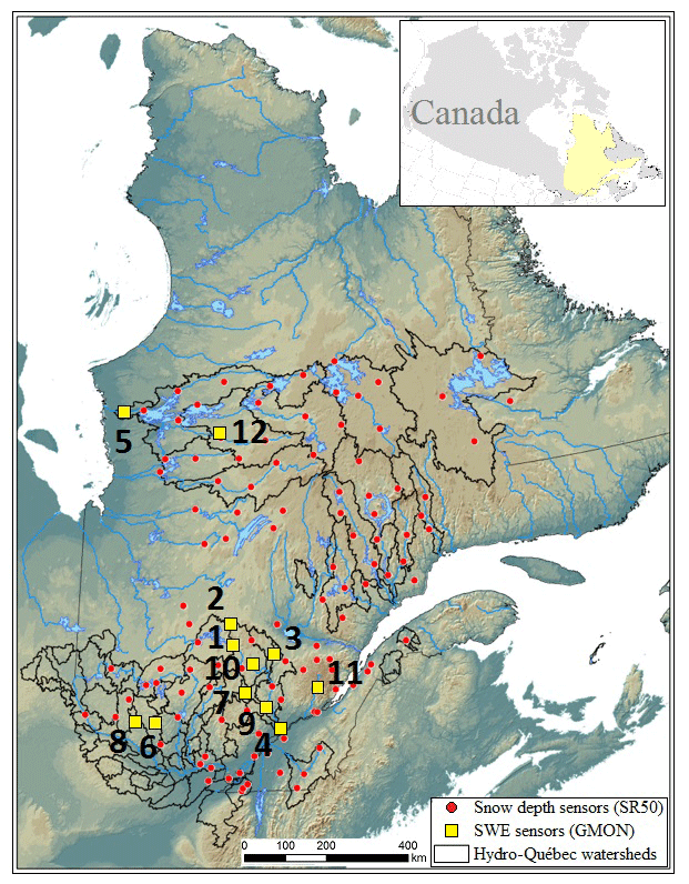
Figure 1SWE measurement stations with the “GMON” SWE sensors (yellow squares; see Table 1 for details) in the province of Quebec. The red circles are the snow depth sensors (“SR50”) used by Hydro-Québec for hydrological purposes, overlaid on a relief map (from blue – low – to brown – higher altitudes) and watershed contours (black lines).
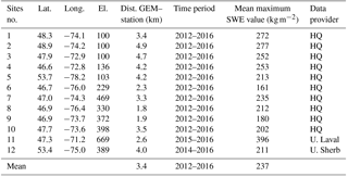
To evaluate SWE simulations, SWE measurements were acquired from 2012 to 2016 by 12 nivometric stations (see numbered stations on Fig. 1), located through a north–south gradient in Quebec. This SWE database (coordinates, sensors, operating period, etc.) was fully described in Larue et al. (2018). Table 1 describes the main station characteristics, including the mean maximum SWE values over operating periods. Daily SWE measurements were derived from gamma ray SWE sensors (Campbell Scientific CS725, “GMON”) with an average error of +5 % (Choquette et al., 2008). Two stations (nos. 5 and 12) were located in the subarctic ecoclimatic zone (53–54∘ N, James Bay area), eight in the coniferous boreal zone (46–48∘ N), and two (Nos. 4 and 11) in a mixed forest area in southern Quebec (45.3∘ N). Sensors were calibrated by Hydro-Québec from numerous field measurement campaigns during the first year following their installation.
A total of 43 winters were studied (Table 1). These winters were all very different. Winter 2012–2013 had the lowest snow accumulation in 10 years (165 cm), whereas winter 2013–2014 was very snowy (379 cm) compared to the average snow accumulation (217 cm). Winter 2014–2015 was unusually cold (3∘ below average temperatures), and winter 2015–2016 was the warmest in 60 years (statistics can be found at http://www.mddep.gouv.qc.ca, last access: 18 October 2018).

Figure 2Methodological scheme describing the DA scheme in the chain of models for SWE retrievals by updating perturbed atmospheric forcing data and snowpack states (“Ft” and “xt”, respectively; see Sect. 3.4).
Table 1Characteristics of the nivometric SWE stations: site number, latitude (Lat.), longitude (Long.) and elevation (El., a.s.l. in meters) of stations. Dist. GEM–station is the distance between the station and the center of the associated GEM grid cell (with GEM, Global Environmental Multiscale weather prediction model; Sect. 2.2). The time period of observations, average of the maximum observed data over the studied period, and data provider are given (HQ: Hydro-Québec, U. Sherb: University of Sherbrooke, U. Laval: University of Laval).
2.2 General setup
Figure 2 shows the general methodology developed to simulate and to assimilate AMSR-2 satellite observations into the snowpack model.
To simulate the signal measured by satellite sensors at the top of the atmosphere (TB TOA), a chain of models was implemented and calibrated over eastern Canada. The 3-hourly continuous atmospheric forcing database provided by the Global Environmental Multiscale weather prediction model (referred to as “GEM”; Coté et al., 1998) was used to drive the multilayer Crocus snowpack model (described in Sect. 3.2.1). Each GEM grid cell has a spatial resolution of 10×10 km2, which is on the same order as the observation scale. The Crocus model updates the snowpack every 15 min by interpolating meteorological inputs, but in this study we used daily Crocus outputs (SWE, snow depth, density, etc.) computed at 14:00 local time (19:00 UTC), in agreement with the AMSR-2 pass (Sect. 3.1.1). The DMRT-ML radiative transfer model (Sect. 3.2.1), driven with Crocus outputs, was used to simulate the PMW emission from the modeled snowpack (referred to as “TBsnow”) at 11, 19, and 37 GHz, at vertical and horizontal polarizations (“V-pol” and “H-pol”, respectively). The contribution of the atmosphere was estimated by using an atmospheric model (Liebe, 1989) driven with the total precipitable water integrated over 28 atmospheric layers and provided by GEM (Sect. 3.3). The surface emissivity for a rough soil was deduced by calibrating the Wegmüller and Mätzler (1999) soil model, and vegetation contributions were quantified with the (ω-τopt) radiative transfer model (Sect. 3.3). To take canopy emissivity variability into account, the inversions of the (ω, τopt) parameters were linked to the 4-day leaf area index (LAI) product from MODIS data (1×1 km2), averaged for each AMSR-2 grid cell (10×10 km2) (Sect. 3.3). These inversions of soil and vegetation parameters were performed over the summer period to avoid bias due to the presence of the snowpack.
The brightness temperatures (TBs) measured by AMSR-2 satellite sensors were assimilated in a DA scheme (see Sect. 3.4). Raleigh et al. (2015) have shown that meteorological forcing data are the major sources of errors in snow model simulations. Hence, we assume here that the uncertainties of GEM meteorological forcing data are the only sources of errors in the TB modeling. It is very difficult to quantify modeling errors due to physical simplifications inside the model due to the spatial scale of the observations. Further studies are needed to estimate these errors over the study area and to take them into account in the DA experiment. The observation error was assumed to be known and the modeling errors were estimated by perturbing selected meteorological forcing variables. An ensemble of 150 TB simulations was obtained and the distribution of these prior estimates represents the modeling error in response to GEM uncertainties. A particle filter with an SIR algorithm was used to update the simulated TB TOA over the winter by adjusting meteorological forcing data and snowpack states (posterior estimates) when an observation was available (Fig. 2).
Several configurations of the DA scheme were tested over three evaluation sites representing different environmental conditions. The best configuration was evaluated over the validation reference sites from 2012 to 2016 (for 43 winters; Sect. 3.4).
Comparing data simulated at the station against model cells involves uncertainty due to spatial variations of the snowpack and land cover. This is a well-known problem for model validation studies and we assume here that the high number of sites (12 SWE stations or 43 snowpack simulations) provides a useful assessment of simulations. It is also known that the spatial localization of measurements can lead to some biases (Molotch and Bales, 2005). To diversify its measurements, Hydro-Québec has installed two SWE sensors in the forest, and not in a clearing as is the usual practice for ease of maintenance.
3.1 Data
3.1.1 AMSR-2 observations
AMSR-2 satellite sensors (Imaoka et al., 2010) provide PMW satellite observations on the 11 (10.7), 19, and 37 GHz channels at V-pol and H-pol. Images produced by AMSR-2 are freely available on the Japan Aerospace Exploration Agency (JAXA) website. This study used the Level 3 Version 2 product, which provides daily TBs normalized on a North Hemisphere polar stereographic projection with a spatial resolution of 10×10 km2 (see https://gportal.jaxa.jp/, last access: 18 October 2018, for the specifications of the projection), from 1 August 2012 to 1 July 2016. TBs from AMSR-2 are computed twice a day: around 13:30 local time, or 17:30 UTC (ascending pass), and around 01:30 local time, or 05:30 UTC (descending pass). Only the ascending pass was used in this study since the snowpack was computed once a day at 14:00 (local time). The use of the ascending pass allowed the nighttime refreezing process to be avoided. To reduce observation errors due to the daytime melting process, the approach was evaluated during the dry snow period, from December to mid-March. This aspect is further discussed in Sect. 5.1.
3.1.2 LAI MODIS data
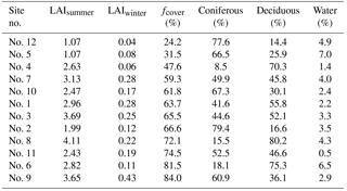
The 4-day LAI product provided by MODIS TERRA data (MOD15A3; Myneni et al., 2002) was used to characterize the vegetation contributions to the total emissivity (Fig. 2). The product has a spatial resolution of 1×1 km2 and was resampled on the AMSR-2 grid of 10×10 km2 by averaging all LAI data within each AMSR-2 grid cell (referred to as “LAIAMSR−2”). For each site, Table 2 describes the summer and winter average values (“LAIsummer” and “LAIwinter”) calculated using LAIAMSR-2 from 1 July to 31 August and from 1 January to 1 March over the 2012 to 2016 time period, respectively (Roy et al., 2014).
Table 2LAIsummer is the mean of the LAI provided by MODIS for the summer period (1 July to 31 August) and averaged over the AMSR-2 grid cell (10×10 km2), LAIwinter is the mean LAI for the winter period (1 January to 1 March). fcover is the fraction of forest cover within the AMSR-2 grid cell extracted from the land cover map Circa 2000 (see Sect. 3.1.3). The percentages of coniferous, deciduous, and water areas are the percentages distributed within the fcover. Sites are ranked in the increasing order of fcover. The three highlighted sites (gray cells) are the sites selected to test the configuration of the DA scheme in Sect. 3.4.3.
3.1.3 Land cover map of Canada
The land cover map of Canada Circa 2000 (available at http://www.geobase.ca/geobase/en/data/landcover/index.html, last access: 18 October 2018) (referred to as “LCC”) was used to extract the fraction of forest cover (“fcover”) within each AMSR-2 grid cell. This product provides the percentage of coniferous, herbaceous, deciduous, and water areas with a spatial resolution of 1×1 km2 and was resampled to generate average values within each 10×10 km2 AMSR-2 grid cell. Table 2 shows the fractions of forest cover provided by the LCC and resampled over AMSR-2 grid cells for each site. As expected, Sites 5 and 12, which are located in the subarctic area (Fig. 1), have a low fcover (below 32 %). The other sites in boreal areas have an fcover of up to 60 %. Sites 6 and 9 are in particularly densely forested areas, with a high fcover (up to 80 %). The measured TB signal can be significantly affected by the forest and the signature of the underlying snow is attenuated during the winter period in such densely forested areas. The sensitivity of the DA scheme to the fcover was analyzed for sites with an fcover above and below 75 % (Sect. 4.2.1).
Moreover, the presence of lakes can affect the PMW signal. Lake ice (when snow cover is absent) increases the PMW signal at high frequencies, and at low frequencies, the contribution of water bodies acts as a reflector and the emissivity remains low (De Sève et al., 1999). With snow cover on lakes, the different snow states on the lakes compared to snow cover under forest also modified the emitted signal (see Derksen et al., 2012, 2014). Nevertheless, we made the hypothesis that these impacts were negligible over our studied sites, which have lake water fractions under 7 % within their AMSR-2 grid cells (Table 2) (masks are generally applied for water fractions of up to 20 %; Takala et al., 2011).
3.2 Simulation of the PMW emission from the snowpack
3.2.1 Coupling of Crocus and DMRT-ML
The chain of models developed to simulate TBsnow is identical to that of Larue et al. (2018), so only a brief description of the approach is detailed here (see Fig. 2).
The Crocus snowpack evolution model (Brun et al., 1989, 1992; Vionnet et al., 2012) is coupled with the ISBA land surface model within the SURFEX interface (Surface Externalisée, in French) (Decharme et al., 2011; Masson, 2013). SURFEX/ISBA/Crocus (hereafter referred to as “Crocus”) computes the evolution of the physical properties of the snowpack and the underlying ground (soil). In particular, the snow layers are modeled with a set of variables representing the morphological properties of snow grains (shape and size), including the specific surface area (SSA), which is one of the most sensitive variables for snowpack emission simulations. The snow microstructure evolves in time according to semi-empirical laws (Vionnet et al., 2012). Crocus is the only model able to simulate the SSA as a prognostic variable (rather than as a diagnostic variable) by using the formulations of Carmagnola et al. (2014). The number of snow layers is dynamic and evolves with physical properties updated at each time step. The maximum number of simulated snow layers was fixed at 15 in this study as a compromise between accuracy and computing time (not shown). Configuration and initialization of the Crocus snowpack model are the same as described in Larue et al. (2018).
TB snow was computed by driving the radiative transfer model DMRT-ML with Crocus outputs. The DMRT-ML model is well detailed in the literature (Tsang et al., 1992; Tsang and Kong, 2001; Picard et al., 2013, Royer et al., 2017), so only the calibration is described here. Snow grain size, and more generally snow microstructure, are factors that most affect the accuracy of simulated PMW emission from a snowpack as they determine the strength of scattering mechanisms in the snowpack at the high frequencies used (Roy et al., 2013; Leppänen et al., 2015; Sandells et al., 2017, Larue et al., 2018). In DMRT-ML, snow grains are represented as spheres of ice with variable interactions between them. The potential formation of clusters of grains, which increases the effective snow grain size, is not taken into account, generating uncertainties (Picard et al., 2013). Several studies have shown that DMRT-ML needed an effective scaling factor to represent the stickiness between snow grains and to correct the snow microstructure representation (Brucker et al., 2011; Roy et al., 2013; Royer et al., 2017). Larue et al. (2018) have shown that a mean snow stickiness parameter (τsnow) of 0.17 was optimal to simulate TBsnow over boreal snow in Quebec (RMSE of 27 K) when DMRT-ML is driven by Crocus snow profiles. This constant τsnow value was thus used in the implemented chain of models (Sect. 3.4.3; Experiment A and B). Nevertheless, this effective parameter could change with snow type (Royer et al., 2017; Larue et al., 2018). Hence, the quality of the DA scheme with the use of the τsnow parameter as a free variable was studied (Sect. 3.4.3, Experiment C).
3.2.2 Ice lens detection algorithm
Since ice lenses (“ILs”) within a snowpack significantly reduce TB mainly at H-pol (Montpetit et al., 2013; Roy et al., 2016), ice layers must be detected and added in the simulated Crocus snow profiles to improve TBsnow simulations. TB in H-pol are much more attenuated by the presence of an IL than TB in V-pol, since the coefficient of reflectivity is stronger in H-pol (Montpetit et al., 2013). Therefore, by following the daily evolution of the PMW emission from the snowpack with AMSR-2 observations, the formation of an IL can be detected by using a threshold on the polarization ratio (PR) defined by Cavalieri et al. (1984) for a given frequency (ν):
In this study, an IL was added on the top of the simulated snowpack if the AMSR-2 PR(11) was above 0.06 (Roy, 2014). This IL was represented as a 1 cm layer with a density of 900 kg m−3 and with the snow grain radius set to zero (Roy et al., 2016). The difficulty is to know how to evolve this IL in the snowpack. The Crocus snowpack model has not yet been adapted to integrate the formation of ILs and evolve them in a coherent way (Quéno et al., 2016). Nevertheless, it was shown in Larue et al. (2018) (from field measurements) that an IL of 1 cm located at 4 cm from the surface of the simulated snowpack minimized the bias of DMRT-ML simulations due to the presence of an IL (regardless of its real location in the snow profile). Hence, the IL first added at the surface of the snowpack was moved to 4 cm from the surface as soon as snowfall was detected with GEM precipitation data or, if not, after 5 days to take into account the snowpack transformations (percolations, sublimations, etc.). The maximum number of detected IL was fixed at two. When a second IL was detected (IL2), IL2 was added at the surface while the first detected IL (IL1) was left at 4 cm. After the next snowfall (or after 5 days otherwise), IL1 was moved to 8 cm from the surface and IL2 to 4 cm. For instance, during winter 2014–2015, one IL was detected at Sites 1 and 12 (22 and 15 December 2014). At Site 9, two ILs were detected: one on 10 December 2014 and another on 1 January 2015.
This is a simplified way to take into account the presence of ILs, and further studies are needed to dynamically evolve these ILs in the snowpack and to model the impact on the neighboring layers. This work is particularly complex, and no solution has yet been found (D'Ambroise et al., 2017), in particular because measurements are difficult to take.
3.3 Simulation of the PMW emission at the top of the atmosphere
The PMW brightness temperature (TB, TOA) emitted at the scale of the AMSR-2 product can be written for each grid cell as
where TB atm↑ is the ascending atmospheric contribution, estimated using the Liebe (1989) model implemented in the Helsinki University of Technology (HUT) snow emission model (Pulliainen et al., 1999). The model considers radiative transfer through the atmospheric layers and provides TB atm↑ values at the satellite sensor level (Liebe, 1989) according to the precipitable water integrated for all atmospheric layers provided by GEM. fseason is the seasonal (winter or summer) fraction of forest cover in the AMSR-2 grid cell, TB forest is the PMW emission with vegetation contributions, and TB open is the PMW emission without vegetation contributions.
The fcover values provided by the LCC map were constants, whereas these fractions of forest evolve with the season. To take into account the temporal evolution of the forest cover for the winter and summer periods (defined as the time period with and without snow, respectively) and to estimate the fseason used in Eq. (2), fcover was linked respectively to LAIwinter and to LAIsummer by comparing the fcover map to the two resampled maps (both resampled on the AMSR-2 projection) throughout Quebec (not shown). The seasonal fractions of fcover were related to seasonal LAIs with Eqs. (3) and (4) for summer and winter, respectively:
The linear correlation between the fsummer values estimated from the LCC and the fsummer values fitted to LAI data with the Eq. (3) had a coefficient correlation R equal to 0.94 and a p value below 0.01. For the LCC fwinter values and the fwinter values fitted to the LAI data (see Eq. 4), the coefficient correlation R was equal to 0.95 and the p value was below 0.01.
3.3.1 Vegetation contributions
The PMW emission from the vegetation varies with the forest characteristics, such as the biomass, the structure of the vegetation, or the liquid water content of the canopy. In this study, the vegetation contribution was modeled with the simplified radiative transfer model (ω-τopt) (Mo et al., 1982), in which the parameters should be estimated by fitting the simulated TBs with observations (Grant et al., 2008; Roy et al., 2012). The ω is the single scattering factor of the albedo. Given the incidence angle θ=55∘ of AMSR-2 satellite sensors, the optical thickness of the vegetation τopt was a function of the forest transmissivity (γ) such that ). The forest transmissivity varies with the frequency (ν) used and is further called γν. At the satellite sensor, the expression of TB TOA in boreal areas was described by Eq. (2), which can be detailed with Eqs. (5) and (6) (see Roy et al., 2012):
where Tsurf is the surface temperature, esurf is the surface emissivity under the canopy (with or without snow) for a given frequency, and Tveg is the temperature of the vegetation (taken as equal to the air temperature at 2 m, provided by GEM). TB atm↓ is the descending atmospheric contributions and γatm is the transmittance of the atmosphere. These atmospheric contributions were modeled using the Liebe (1989) model, as were the TB atm↑ values. Thus, for snow-free conditions, only forest (ω, γν) and soil (esurf) parameters were unknown and needed to be adjusted for each site by fitting the model output to the observations.
3.3.2 Soil contributions
To deduce the surface emissivity for rough soil (esurf, p for a given polarization p), the Wegmüller and Mätzler (1999) soil model was used to calculate the surface reflectivity of rough soil under the canopy (rsurf, p for a given polarization p), with or without snow by using Eqs. (7) and (8):
where rsurf, p mainly depends on the surface roughness and Fresnel coefficients (ΓFresnel, H). In Eq. (7), the simplified parameter σs=kσ was used, where k is the wave number and σ the standard deviation of the surface height (in meters); α is a constant parameter fixed to −0.1 (Wegmüller and Mätzler (1999). For frozen soil, parameters derived from Montpetit et al. (2018) were used (see Sect. 4.1). For thawed soil, ΓFresnel, H was estimated from the dielectric constant calculated with the Dobson (1985) equations according to the soil moisture and soil temperature. These variables were computed with the Crocus model, coupled to the ISBA land surface model, and extracted daily (at 14:00, as the other variables). The soil reflectivity in vertical polarization also depends on a parameter βν (Montpetit et al., 2018), which describes the polarization of the signal and is frequency-dependent. Note that we will often use the “ν” subscript hereafter to denote quantities that are dependent on frequency.
Hence, the soil parameter esurf was linked to the set of values (σs, βν) and mainly evolved with soil moisture and soil temperature.
3.3.3 Inversions of vegetation and soil parameters
The inversion of forest (ω, γν) and soil (σs, βν) parameters was carried out in summer to avoid the bias due to the presence of a snowpack. Forest parameters (ω, γν) depend on the forest characteristics, such as the biomass and the structure of the canopy at each site. They also depend on LAI, which allows the season forest emission cycle to be accounted for. Using the vegetation water content equation defined by Pampaloni and Paloscia (1986), the parameter γν was related to the 4-day LAI for a given frequency ν with the Eq. (9):
where a and b are two constants to calibrate. To reduce the number of unknown variables, Eq. (9) was simplified to use only one constant ην such as .
The vegetation and soil parameters were inverted by minimizing the difference between TB TOA simulations and TB TOA measured with AMSR-2 sensors at 11, 19, and 37 GHz in vertical polarizations. We used the same approach developed by Roy et al. (2014) since it was well adapted for PMW emission in boreal areas: the two frequency-dependent parameters (ην,βν) and two frequency-invariant parameters (ω, σs) were inverted with a two-stage calibration by permuting all possible combinations of the two frequency invariant parameters. Specifically, ω values varied from 0.02 to 0.16 in steps of 0.01, and σs varied from 0.01 to 1.1 in steps of 0.05. This yields a total of 300 possible combinations of the frequency invariant parameters. Then, for each possible combination of the frequency-invariant parameters, a calibration of the frequency-dependent parameters, ην and βν, was performed for each frequency. A total of 900 frequency-dependent calibrations were thus computed. Finally, for each possible combination of the frequency-invariant parameters, the total post-calibration TB RMSE across all three frequencies was computed. The combination of frequency-invariant parameters resulting in the lowest TB RMSE was chosen.
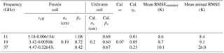
TB TOA were simulated from 2012 to 2016. The inversion was not very sensitive to σs (not shown) and Fig. 3 shows the optimal overall TB TOA RMSE between simulated and measured TB TOA for the 12 sites and for the summer period according to ω values. Over the summer period, a ω value at 0.07 and a σs value at 0.2 cm gave best results for TB TOA simulations, with a minimum overall RMSE equal to 9.0 K. These parameters were previously optimized over the same study area by Montpetit et al. (2018). A value of ω=0.07 was coherent with the literature for dense boreal forest areas (Pellarin et al., 2006; Meissner and Wentz, 2010; Roy et al., 2012). For this optimal (ω, σs) set of values, the mean optimal values of the ην and βν factors were estimated, by considering the soil contribution constant if the soil was frozen.
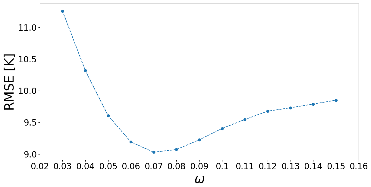
Figure 3Overall TB RMSE (at 11, 19, and 37 GHz, for the 12 sites and for the summer period) between the simulated and measured TB TOA as a function of the values of ω. A σs value at 0.2 cm gives the best results but TB RMSE is not very sensitive to this variable. The parameters βν and ην were optimized for each (ω, σs) couple according to the frequency used.
3.4 Data assimilation setup
The DA setup is the same as the one developed in Larue et al. (2018) except that we added an inflation technique of the covariance matrix of observation errors (R matrix) to avoid ensemble degeneracy, i.e., when an ensemble collapses to a unique particle (Arulampalam et al., 2002).
3.4.1 DA framework
The DA scheme is a particle filter with a Sequential Importance Resampling algorithm (PF-SIR) that is well documented in Van Leeuwen (2009, 2014) and Gordon et al. (1993) and relatively easy to implement with a snowpack model (Dechant and Moradkhani, 2011; De Lannoy et al., 2012; Charrois et al., 2016; Larue et al., 2018). The PF-SIR represents the probability density function (pdf) of the model state with an ensemble of states (called particles), which is updated when an observation is available. An ensemble approach was preferred because of the nonlinearity of the system. Moreover, the particle filter approach can cope with the variable number of state variables resulting from the changing number of snow layers in Crocus. The created ensemble represents uncertainty in SWE and in TB simulations due to the uncertainties of meteorological inputs (Fig. 2).
Assuming that the meteorological forcing data were the only source of uncertainties, the ensemble of TBs was created by running the chain of models described in Fig. 2 with an ensemble of perturbed inputs. The assimilation was performed daily (at 13:00) and the ensemble was composed of 150 members, which was found to be an adequate size (Larue et al., 2018). The daily ensemble of meteorological forcing data was created by perturbing selected GEM data (air temperature, wind speed, precipitation, and short- and long-wave radiation) with Gaussian noise according to their respective uncertainties (estimated in Larue et al., 2018). Meteorological forcing perturbations were propagated in time following a first-order autoregressive process to simulate their realistic temporal variations (Charrois et al., 2016). Precipitation, wind speed, and short-wave radiation (“SWdown”) were perturbed by a multiplicative factor centered at 1. Perturbation boundaries were fixed at −0.9 and 0.9. The air temperature was perturbed by an additive factor, with boundaries fixed at −3 and +3 K. Perturbed long-wave radiation (“LWdown”) was estimated with perturbed Tair from a linear regression estimated in Larue et al. (2018). In order to maintain physical consistency in the simulations, SWdown was limited to 200 W m−2 when there was precipitation (presence of clouds) (Charrois et al., 2016).
The observation error standard deviation associated with AMSR-2 observations was assumed to be 2 K (Durand and Margulis, 2006, 2007). Note that in reality it was probably larger since it represents all mismatches between observations and simulations obtained if the model was run with “correct” inputs. This observation error cannot be easily estimated (low spatial resolution, representativeness, etc.), but it is only a sort of initial value here, since we used a covariance inflation to adjust it.
DA experiments were applied between 1 November and 1 May. To avoid wet snow conditions, which increase the emissivity of the snowpack, whereas the SWE does not change, the DA was not performed when liquid water content was observed in the modeled snowpack. This variable was computed by Crocus, driven with original meteorological forcing data. SWE values were evaluated over both the dry snow period (from 1 December to 15 March) and the whole winter (when a snowpack was detected).
3.4.2 DA and inflation technique
The snowpack prior state xt at time t is computed with the updated past state of snowpack simulations at time t−1 (posterior state xt−1) and the prior perturbed meteorological forcing data Ft from time t−1 to t (see Fig. 2). The predicted observation is computed with
where is TB TOA predicted from particle i (i=0 … N, with N the ensemble size). The observation operator h is the τsnow-calibrated DMRT-ML model and the calibrated radiative transfer models estimating soil, atmosphere, and vegetation contributions. In the analysis step, the new posterior distribution is updated by weighting each particle according to the distance between and the AMSR-2 TB observation (with the weight we). With the SIR algorithm, the pdf is resampled by duplicating particles with high weights (i.e., close to observations) and dropping with negligible weights (far from observations). With Arakawa's procedure used here for ensemble resampling (Arakawa, 1996; same as Charrois et al., 2016), a particle is definitely selected if its weight is higher than or equal to the inverse of the ensemble size (we, with N=150).
Ensemble resampling considerably reduces the risk of degeneracy but does not eliminate it. Degeneracy starts when only a few particles have significant weights. These particles are selected many times, leading to a loss of diversity of the posterior ensemble. After several assimilation steps, the ensemble quickly reduces to a single particle. Ensemble degeneracy can be detected when the number of selected particles (those with high weights) is below an effective limit number Nkeep, here fixed at 25 as a compromise between the quality of the DA scheme and the size of the ensemble (not shown). In this study, we developed a new technique to avoid a degeneracy problem, which consists in the online adjustment of the R matrix (i.e., observation standard deviation squared times the identity matrix) such that the weight of the 25th selected particle (wekeep) is at least equal to 1∕N. The rationale here is that, because the weights are nonlinear functions of the observation error covariance matrix, a larger matrix tends to flatten the distribution of weights and favors the selection of more particles. This adjustment is performed with an inflation of the initial matrix, and the detailed algorithm is provided in Appendix A.
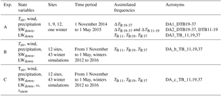
Table 3Experiment setup information. Exp. is the experiment identifier (see text). TBs are in V-pol.
Ensemble degeneracy is often caused by extreme precipitation events resulting in very high TB values difficult to represent with the model. The online adjustment technique mitigates the consequences of this model deficiency on the snow simulations over the rest of the season. The other side of the coin is that a “good” observation can be ruled out if the model is not able to reproduce it, thereby reducing the accuracy of the snowpack estimation.
3.4.3 Experimental setup
To study the sensitivity and the quality of TB assimilation for SWE improvements, three experiments were performed.
(a) Experiment A: to test the feasibility of the DA scheme for several environmental conditions, and to find the best DA configuration to apply, TB assimilation for three representative sites was performed in a preliminary experiment for winter 2014–2015. Following a north–south gradient, we selected Site 12 (fcover=24.2 %, northern coniferous area), Site 1 (fcover=63.7 %, coniferous area), and Site 9 (fcover=84.0 %, mixed forest area), each representing a different environmental condition. Over these three sites, we estimated the quality of the DA scheme according to the assimilated frequencies: (a) assimilation of the TB difference between 19 and 37 GHz (referred to as ΔTB 19-37); (b) assimilation of the ΔTB 19-37 and the TB difference between 11 and 19 GHz, in V-pol (referred to as “ΔTB 11-19”); and (c) assimilation of the three TBs at 11, 19, and 37 GHz in V-pol (TB 11, TB 19, TB 37). Table 3 summarizes the experiment setup information (acronyms of the experiments, sites, time period). We used V-pol TB because H-pol TB is more sensitive to the stratigraphy of the snowpack and to the presence of ILs (Mätzler, 1987). While the DA of TBs at 11, 19, and 37 GHz in V-pol should give best results since this combination of frequencies imposes more constraints, the risk of encountering a degeneracy problem is higher. The combination of both ΔTB 19-37 and ΔTB 11-19 is commonly used in the literature for SWE retrievals (Chang et al., 1987; Tedesco et al., 2004; Tedesco and Nervekar, 2010). The assimilation of the ΔTB 19-37 only was also studied to analyze the sensitivity of TB assimilation for deep snowpack when TB 37 saturates for a SWE up to about 150 mm (Mätzler et al., 1994) and to evaluate the supply of information from 11 GHz in the assimilation of both ΔTB 19-37 and ΔTB 11-19 for SWE improvements.
To quantify the performance of the DA scheme, the daily RMSEs of ensembles of simulated SWE obtained with and without the DA scheme were compared by using Eq. (11):
where N is the ensemble size, Xsim i, t is the simulated variable from the member i at time t, and XObs t is the diagnostic variable at time t obtained from AMSR-2 observations.
Table 4Effective parameters calibrated for the 12 studied sites to quantify soil contributions esurf (calibrated surface roughness “cal. σs” and calibrated polarization ratio “cal. βν”) and vegetation contributions (controlled by the calibrated (ω, ην) parameters “cal. ω” and “cal. ην” according to the daily LAI) measured at the top of the atmosphere. The parameterization of frozen ground was estimated by Montpetit et al. (2018). εeff is the effective dielectric constant estimated with the permittivity of frozen and unfrozen soils derived from Dobson's equations (1985). Annual and seasonal TB TOA RMSEs estimated for the summer and the winter period (RMSEsummer and RMSEwinter) are calculated from 2012 to 2016 with the calibrated parameters.
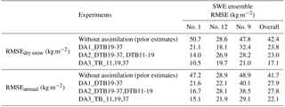
(b) Experiment B: the best configuration of the DA scheme (DA of the three TBs at 11, 19, and 37 GHz in V-pol, called the “DA_b_TB_11, 19, 37” experiment in Table 3) was applied over the 43 winters. To estimate the accuracy for hydrological applications, the median of the resampled SWE ensemble obtained with the DA_b_TB_11, 19, 37 experiment (called “SWEDA”further) was compared to SWE measurements. The median was used instead of the mean to reduce the potential impact of extreme perturbations. The evaluation of this experiment was performed by comparing SWEDA RMSE and the relative percentage of error (“RPE”) values to the original SWE simulations (SWECrocus), obtained by driving Crocus with original meteorological forcing data. The RPE is defined as
The mean biases of SWE estimates obtained without and with assimilation were also compared. Performance was estimated for SWE higher than 48 kg m−2(about 20 cm of snow depth), derived from measurements, to attenuate problems of shallow snow cover variability or heterogeneity in the AMSR-2 grid cells. To analyze the impact of the vegetation, results were separated according to the fraction of fcover: moderate fcover (fcover < 75 %, 10 sites) and high fcover (fcover > 75 %, 2 sites) (see Table 2 for fcover site information).
The accuracy needed for hydrological applications is a SWE RPE lower than 15 % (Vachon, 2009; Larue et al., 2017), which is the same performance objective as the CoreH2O project (10 % for SWE >30 cm and 3 cm for SWE <30 cm, Rott et al., 2010) and the GlobSnow2 product (Luojus et al., 2014). This error threshold corresponds to an RMSE of about 45 kg m−2 for a measured average Quebec snowpack about 300 kg m−2 of SWE. The ability to accurately estimate the annual SWE maximum (SWEmax) was also studied since it is one of the most important variables for hydrological applications. It allows the amount of water stored in the snowpack before the spring snowmelt to be described. To avoid extreme values, the SWEmax is estimated as the average of the SWE for a time period of ±2 days around the detected SWEmax.
(c) Experiment C: the quality of the DA scheme could strongly depend upon the choice of state variables. In the A and B experiments, we chose to pre-calibrate forest and soil parameters and to use a constant snow stickiness parameter (τsnow) fixed at 0.17 (Larue et al., 2018). Nevertheless, these calibrations are empirical and should be adjusted for each site. It depends on several parameters that are difficult to measure at a 10×10 km2 spatial scale (snow grains, canopy, biomass, etc.). The forest parameter ω strongly affects the PMW emission from the vegetation, which can represent more than 60 % of the signal measured by satellite sensors (see discussion in Sect. 5.2). Kwon et al. (2017) have shown that the contribution of TB Veg to TB TOA was better represented by considering ω free in the DA scheme, and improvements in the resulting SD were evident for the forest land cover type (about 5 % with DMRT-ML). In Experiment C, the DA scheme was thus tested using ω and τsnow as free variables in the assimilation process (called the “DA_c_TB_11,19,37” experiment). The DA_c_TB_11,19,37 experiment is identical to the DA_b_TB_11,19,37 experiment (over the 43 winters); only the state variables were changed. The ω parameter was perturbed with Gaussian noise, centered on 0.07 (as calibrated), with a standard deviation of 0.02 and bounded by 0.05 and 0.12 (reasonable range of TB TOA RMSE values; Fig. 3). The snow stickiness parameter was perturbed by Gaussian noise, centered on 0.17, with a standard deviation of 0.15 and bounded by 0.1 and 0.46. These limits correspond to the range of τsnow values extracted from Larue et al. (2018) over the same study area. The ensemble size was kept to 150 members.
Table 5Averaged SWE ensemble RMSE (see Eq. 11) obtained with and without DA, according to the experiment (see Sect. 3.4.3, Table 3 for acronyms) for each tested site. RMSEdry-snow is the SWE ensemble RMSE obtained from 1 December to 15 March. RMSEannual is estimated over the whole winter (when snowpack is detected). No. corresponds to the site (see Table 1).
4.1 Results of model inversions
The mean optimal values of the ην and βν factors were estimated for the optimal (ω, σs) set of values (0.07 and 0.2, respectively; see Table 4). The (σs, βν) soil parameters are given in Table 4 and are used to estimate the TB TOA RMSE obtained with the calibrated chain of models. Without parameter inversions, the annual mean RMSE of the original TB simulations varies from 12.9 to 47.1 K for the three frequencies (not shown). With parameter inversions over the summer period, the three frequencies have a similar TB RMSEsummer (8.6–10.1 K, Table 4), while over the year (using parameters inverted over the summer period) the annual TB TOA RMSE significantly increases at 37 GHz due to the presence of the snowpack (26.0 K). The inversions make it possible to reduce the annual TB,37 RMSE by 21.1 K. Figure 4a, b, and c show the multiyear TB TOA variations for Sites 12, 1, and 9, respectively, from 2012 to 2016 and at 37 GHz. At this frequency, the simulated TB TOA is strongly underestimated when a snowpack is observed. This is likely due to an overestimation of the SWE or snow grain sizes since TB,37 are attenuated in the snowpack as snow grains act as diffusers while the TB,19 and TB,11 are relatively unaffected by snow grains (RMSEsummer similar to RMSEwinter at 11 and 19 GHz; Table 2). Simulated SWE values were overestimated by 16 % and 20.2 % compared to SWE measurements for Sites 1 and 9, respectively, for winter 2014–2015. The objective of TB assimilation is to reduce these overestimations. Note that the SWE simulated at Site 12 is underestimated by 19 %. The underestimation of TB,37 can also be caused by an underestimation of the vegetation contributions. This aspect is further discussed in Sect. 5.2.
By integrating ILs within the snowpack when the PR11 is above 0.06, the annual TB TOA RMSE at 37 GHz is reduced and goes from 28.9 to 26.0 K.
In winter, the overall TB TOA RMSE (all frequencies) is equal to 17.4 K from 2012 to 2016 (not shown), similar to the overall RMSE estimated for the τsnow-calibrated DMRT-ML driven by in situ measurements in an open area and equal to 19.9 K compared to surface-based radiometric measurements in Quebec (Larue et al., 2018).

Figure 4Multi-year variations of simulated TB TOA (red dotted lines) and measured TB TOA (black full lines) from 2012 to 2016 at 37 GHz in vertical polarization: (a) Site 12 (fcover of 24 %), (b) Site 1 (fcover of 64 %), and (c) Site 9 (fcover of 84 %) (see Table 2).
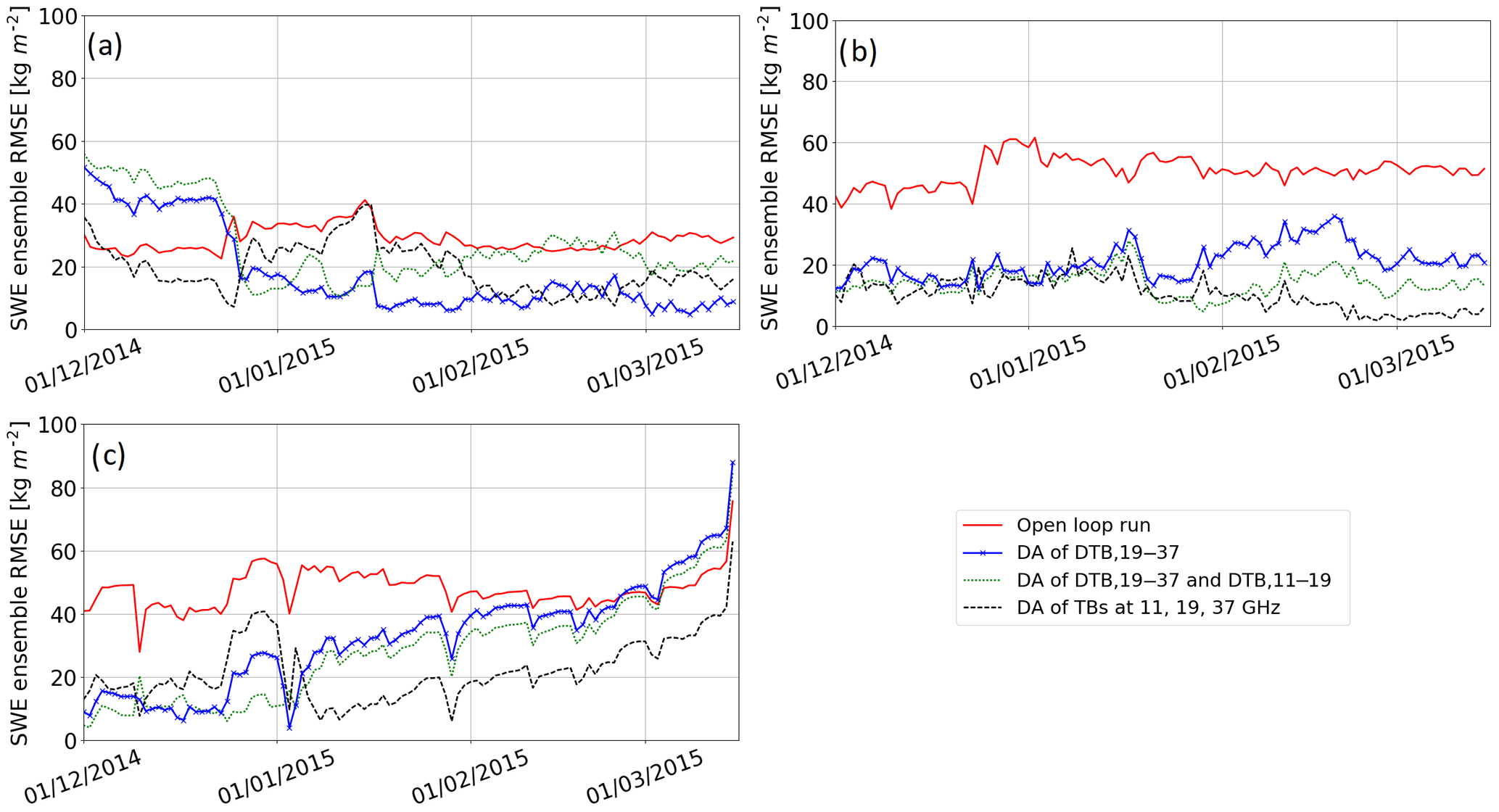
Figure 5Variations of the SWE ensemble RMSE (Eq. 11) obtained with and without DA for the dry snow period (from 1 December to 15 March). Experiments are performed for (a) Site 12, (b) Site 1, and (c) Site 9, over the winter 2014–2015. The red line is the SWE ensemble RMSE obtained without DA (open loop runs), the blue line is the RMSE obtained with the DA1_TB19-37 experiment, the green dashed line the RMSE with the DA2_TB19-37,TB11-19 experiment, and the black dotted line the RMSE with the DA3_TB_11,19,37 experiment.
4.2 Results of AMSR-2 data assimilation (DA)
4.2.1 Experiment A
Figure 5 shows variations of the daily RMSE of the SWE ensemble (see Eq. 11) obtained without and with DA (prior and posterior estimates) according to the combination of frequencies used as observations (DA1_DTB19-37, DA2_DTB19-37, DTB11-19 and DA3_TB_11,19,37 experiments; see Table 3). Table 5 summarizes these averaged RMSEs for the studied period (dry snow period and whole winter) for tested sites.
Over the three sites and for the dry snow period, the DA reduced the overall SWE ensemble RMSE by 43.9 %, 45.8 %, and 59.7 % with the DA1_DTB19-37, DA2_DTB19-37,DTB11-19, and DA3_TB_11,19,37 experiments, respectively, compared to the SWE ensemble RMSE obtained with prior estimates (Table 5). The assimilation of the three frequencies (DA3_TB_11,19,37) helps to improve SWE simulations, giving the lowest RMSE compared to other scenarios. The same trend is observed over the whole winter and the assimilation of the three frequencies reduces the overall SWE ensemble RMSE by 47.0 % (SWE ensemble RMSE of 22.1 kg m−2) compared to the SWE ensemble RMSE of prior estimates (SWE ensemble RMSE of 41.7 kg m−2).
In our previous work (Larue et al., 2018), we have shown a reduction of 82 % of the SWE RMSE by assimilating both the ΔTB 19-37 and ΔTB 11-19 and using synthetic observation data over a dry snow period. The differences between results using synthetic and real data in DA experiments are likely due to two aspects. Firstly, the snow model does not resolve the intra-pixel surface variability. We assumed homogeneous snow cover within the pixel in open areas, thus with no interactions between snow and vegetation. Even if we compare simulations with surface-based measurements in open areas, this could introduce large uncertainties (Roy et al., 2016). Secondly, the land cover variability and heterogeneity within each pixel also induce uncertainties in the mean TB simulation over a pixel (TB weighted by the fraction of forest cover; see Eq. 2).
Table 6Averaged SWE RMSE, bias, and RPE (Eq. 12) over the 43 winters for original SWE simulation (SWECrocus) and assimilated SWEDA(Experiment B). Statistical performances were estimated for SWEobs>48 kg m−2 (snow depth higher than ∼20 cm). and are the averaged observed and simulated SWE, respectively.
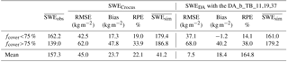
Figure 6 illustrates the comparison between SWE measurements, the original SWE Crocus simulations (SWECrocus), and the median of the SWE ensemble obtained with the DA3_TB_11,19,37 experiment. The yellow envelope corresponds to the SWE ensemble obtained without DA (prior estimates) and shows a large ensemble spread in response to meteorological forcing uncertainties. The gray envelope is the resampled SWE ensemble (posterior estimates). SWE simulations are very sensitive to the uncertainties of meteorological forcing data at the beginning of the winter season. If an event (melting or precipitation) is missed, a constant bias on SWE estimates is kept throughout the winter. For Sites 1 and 9, the DA scheme allows the correction of these uncertainties at the beginning of the season: the SWE ensemble RMSEs of posterior estimates are reduced by about 30 kg m−2 at the beginning of the season, compared to the RMSE of prior estimates (Fig. 5). For these two sites, the SWE ensemble RMSE obtained with the DA1_DTB19-37 experiment increases as the snowpack becomes deeper, especially from mid-January when the snowpack becomes deeper than 100 kg m−2 (Fig. 6). The PMW signal from the snowpack at 37 GHz saturates for such deep snowpack (Mätzler et al., 1982; Mätzler, 1994; De Sève et al., 1997, 2007) and the assimilation of only does not give enough information to significantly improve SWE retrievals. For Site 9, posterior estimates are deteriorated at the end of the season compared to prior estimates with the DA1_DTB19-37 experiment. By adding (DA2_DTB19-37,DTB11-19), this effect is reduced but stays sensitive to the depth of the snowpack (Fig. 5).
Note that the gray envelope does not always include the observations (Fig. 6a, c). This could be due to an under-estimation of the R matrix. In the developed approach, the inflation technique of the R matrix is limited by a threshold on the α factor fixed at 5 since the simulations are limited by the simplifications of physical parameters in the models and we may introduce a bias if we force them to follow the observation by perturbing meteorological forcings only. Further work is needed to quantify the model errors in order to consider it in the DA scheme and to improve the representativeness of the simulations. To represent the uncertainties about the physical processes simulated with the Crocus snow model, a new system based on snow model ensembles could be an alternative. Such an approach was recently developed by implementing different configurations estimating the physical parameters of the Crocus snow model (ESCROC, Lafaysse et al., 2017).
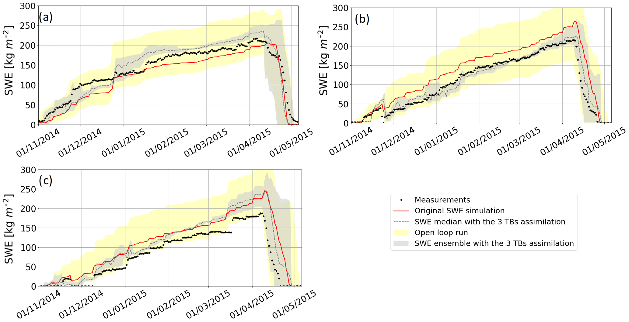
Figure 6Evolution of SWE measurements (black points) and SWE simulations. The SWECrocus is the red line, and the SWE obtained with the DA3_TB_11,19,37 experiment is the gray dotted line. The yellow envelope is the spread of the SWE ensemble obtained with open loop runs (prior estimates). The gray envelope is the spread of the SWE ensemble obtained with the assimilation of the three frequencies (posterior estimates). Both spreads are delimited by the 5th and the 95th percentiles. Experiments are computed for (a) Site 12, (b) Site 1, and (c) Site 9, over the winter 2014–2015.
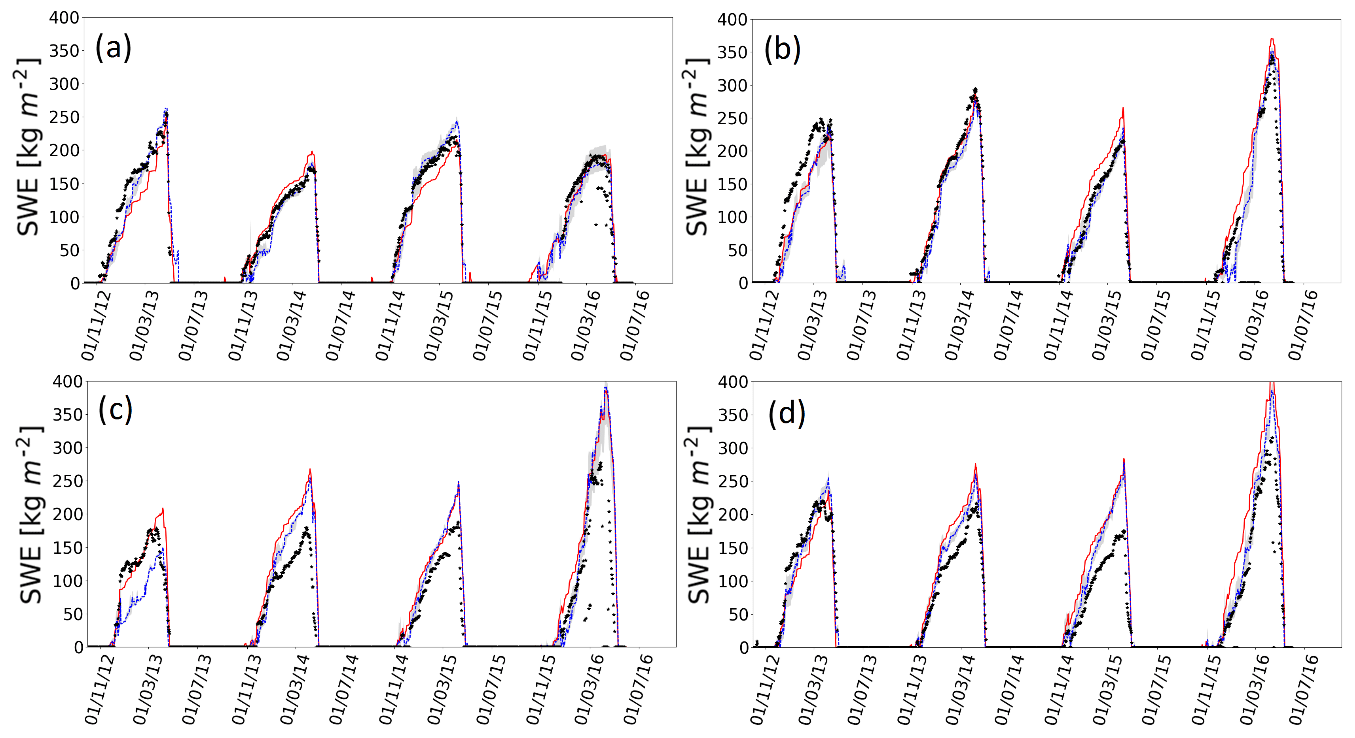
Figure 7Evolution of SWE measurements (black points), original SWE simulations (red full line), and the median of the SWE ensemble obtained with the DA_b_TB_11,19,37 experiment (SWEDA) (blue dotted line). The gray envelope is the spread of the SWEDA ensemble (posterior estimates). Experiments are computed for (a) Site 5 (fcover=31.5 %), (b) Site 1 (fcover=63.7 %), (c) Site 9 (fcover=84 %), and (d) Site 10 (fcover=61.8 %), from 2012 to 2016.
4.2.2 Experiment B
The median of the resampled ensemble of SWE obtained with the DA of the three frequencies (SWEDA) is used to estimate the global performance of the DA scheme for SWE improvements. Table 6 details the statistical performance of simulated SWEDA compared to measurements and to the original SWE Crocus simulations (SWECrocus) over the 43 winters. Figure 7 compares the SWEDA, SWECrocus, and SWE measurements (SWEobs) from 2012 to 2016 for four sites with different fcover taken as an example: Site 5 (fcover=31.5 %), 10 (fcover=61.8 %), 1 (fcover=63.7 %), and 9 (fcover=84.0 %). In this section, we first analyze the overall SWE improvements obtained with TB assimilation compared to original SWE simulations, and the impact of the vegetation on the quality of the DA scheme is discussed.
Overall SWE improvements compared to original Crocus simulations
The overall SWECrocus RMSE, bias, and RPE are of 45.0 kg m−2, 23.7 kg m−2, and 22.1 %, respectively (Table 6). In comparison, the overall SWEDA RMSE, bias, and RPE are improved and equal to 41.2 kg m−2, 7.5 kg m−2, and 18.4 %, respectively. The overall bias is reduced by 16.2 kg m−2 (68 % of SWECrocus bias) with the DA scheme. The DA of the three frequencies thus helps to improve SWE estimates over Quebec. Correlation between SWEDA simulations and SWE measurements gives a similar R coefficient to the one obtained with SWECrocus simulations (R=0.79 and R=0.78, respectively), but the offset is significantly reduced with SWEDA compared to SWECrocus (offset =10 and 29 kg m−2, respectively). We analyzed the number of cases with significant improvements for the total of 43 simulations studied by considering a 5 % threshold on the bias and RMSE differences before and after assimilation. The SWEDA bias is significantly reduced for 26 winters (60 % of cases) compared to original SWE simulations. However, the RMSE is significantly improved for only 35 % of simulations, and in 35 % of cases, RMSEs are similar.
Evaluation of SWEmax
The mean observed SWEmax is equal to 235.6 kg m−2 from 2012 to 2016, and the mean simulated SWEmax is equal to 278.3 and 266.8 kg m−2 without and with the assimilation, respectively. Compared to original SWE simulations, the DA scheme improves 63 % of SWEmax simulations with an overall improvement of 12.2 kg m−2, corresponding to 8 % of SWE measurements (Table 6). Such an uncertainty extended over the whole territory could have a strong impact, considering that 1 mm of SWE in the LG watershed could represent USD 1 million in hydroelectric power production (Brown and Tapsoba, 2007).
SWE accuracy for sites according to the fcover
The overall RPE obtained with the DA scheme is below 15 % (RPE =14.1 %) for sites with an fcover below 75 % (Table 6), which is the accuracy required for hydrological applications (Larue et al., 2017). Hence, the accuracy of SWEDA estimates, obtained without the use of any surface-based data, is very encouraging for hydrological needs in remote areas. In comparison, the GlobSnow-2 SWE product (Takala et al., 2011), which assimilates both TBs and in situ snow depth measurements, has a SWE RPE equal to 35.9 % over the same area in Quebec (Larue et al., 2017), twice the uncertainty of SWEDA. Figure 7a and b (Sites 5 and 1) show that for a single site, the original SWECrocus simulation works well for some years but can be underestimated or overestimated over other years. The DA scheme allows a more stable solution when the overall fcover is under 75 % (not the case for Site 9, for example).
Nevertheless, even if the overall RMSE is improved, the DA scheme does not help to improve SWE estimates for sites with an fcover above 75 % (RMSE of 66 kg m−2) compared to original SWE simulations (RMSE of 62.0 kg m−2). The presence of vegetation is a major source of uncertainty in TB TOA simulations. The emission of the trees is superimposed on the signal emitted by the underlying snowpack and increases the TB measured at the satellite level (Chang et al., 1996; Brown et al., 2003). At same time, the canopy also attenuates the surface emission toward the satellite. These contributions are complex to quantify since it depends not only on the tree fraction within the pixel but also on the tree species and states which emit/attenuate a different PMW signal depending on their biomass (liquid water content), volume, and structure (stem, leaf, trunk) (Franklin, 1987). Also, the presence of trees modifies snow accumulation on the ground, depending on interception, shade, and sublimation effects (Dutra et al., 2011; Wang et al., 2009), which increases the spatial variability of the snowpack within the same pixel. These interactions between the vegetation and the snowpack are not taken into account in Crocus, and this might induce uncertainties due to model errors. Note that SWE sensors are mostly installed in clearings, which reduces this impact in comparisons against surface-based measurements.
Kwon et al. (2016) used a similar snow radiance assimilation system to correct SD by updating the Community Land Model, version 4 (CLM4), snow and soil states, and radiative transfer model with the assimilation of the 19 and 37 GHz of AMSR-E. Over North America, it produced significant improvements of SD for the tundra type, but also produced degradations for taiga snow class and forest land cover (7.1 % and 7.3 % degradations, respectively). In the present study, the use of a multilayer snowpack model makes it possible to represent PMW emission from the snowpack with DMRT-ML well, and to improve overall snowpack simulations with TB assimilation in boreal areas when the fcover is below 75 %. Kwon et al. (2017) obtained better results for areas with a high fcover in comparison to their previous study (Kwon et al., 2016) over North America by using the vegetation parameter ω as a free variable in the DA scheme, instead of pre-calibrating it as we chose to do. This aspect is further studied with the experiment C.
4.2.3 Experiment C
Table 7 shows the statistical SWE performances obtained with the DA_c_TB_11,19,37 experiment (see Table 3 for definitions), where ω and τsnow are taken as free variables in the DA scheme (“SWE”) over the 43 winters.
Table 7Same as Table 6 but using the forest parameter ω and the snow stickiness parameter (τsnow) as free variables in the DA scheme (Experiment C) to improve SWE retrievals (SWE).
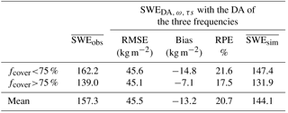
The overall SWE RMSE, bias, and RPE are equal to 45.5 kg m−2, −13.2 kg m−2, and 20.7 %, respectively, very close to the statistical performances of the original SWECrocus simulations. The use of ω and τsnow as free variables does not help to improve SWECrocus simulations for sites with an fcover below 75 %, but the bias is significantly reduced for sites with an fcover above 75 % (−7.1 kg m−2 and a RPE of 17.5 %). In addition, the simulated SWEmax is improved for 86 % of the 43 simulations (37 cases), with a reduction of the SWEmax bias of 26.6 kg m−2 (17 % of SWE measurements) compared to the original SWECrocus simulation.
The use of pre-calibrated parameters is justified because the parameters ω and τsnow were not measurable and could not be directly validated. Furthermore, if parameters are added as state variables in the DA scheme, a larger ensemble size in the DA scheme would be needed to improve the representativeness of TB uncertainties and to ensure the solution's stability (or at least to prevent a degeneracy problem). The ensemble size was kept to 150 here but this DA_c_TB_11,19,37 experiment should produce improved results with a larger ensemble size. However, this would require a significant computational effort. This study is a preliminary step of a PMW DA implementation for operational hydrological applications, so there was a need to limit computing time. These results suggest that the developed approach using pre-calibrated ω and τsnow parameters helps to improve the retrievals for sites with an fcover below 75 %, and the use of ω and τsnow parameters as free variables in the DA scheme should be investigated in further work for sites with more than 75 % forest cover.
In this section, we discuss (a) the sensitivity of wet snow conditions for TB assimilation, and (b) the percentage of surface, vegetation, and atmospheric contributions in the PMW signal measured by satellite sensors.
5.1 Wet snow conditions
In wet snow conditions, water droplets act as emission sources (especially at frequencies above 30 GHz), and the snowpack becomes close to a blackbody (Brucker et al., 2011; Picard et al., 2013; Klehmet et al., 2013). The PMW observations are thus complex to use for SWE retrievals, especially at the end of the season before the spring snowmelt when the SWE is maximal. Figure 8 illustrates the SWEDA obtained with the DA of the three frequencies applied over the whole winter and when the snow is dry only (with an LWC equal to 0 kg m−2), for Site 3 (winter 2013/2014). SWE estimates are strongly deteriorated when TB assimilation is performed in wet snow conditions. For this example, the SWEDA RMSE is equal to 31.1 kg m−2 with a DA performed over the dry snow period only and significantly increases to 70.2 kg m−2 by assimilating TBs over the whole winter (dry and wet snow conditions).
Here we used the LWC simulated by Crocus to detect wet and dry snow. This variable is subject to model errors and is linked to the original atmospheric forcing data and to their uncertainties. Further studies are needed to automatically detect wet snow events by using direct satellite observations. Previous studies have shown the potential to use the gradient ratio (GR =TB 37–) to detect rain-on-snow events in arctic areas (Langlois et al., 2017; Dolant et al., 2016), and this approach should be investigated for boreal forest areas in further work. The use of active microwave observations is also a promising approach with a good spatial resolution (Roy et al., 2010).
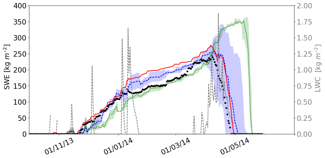
Figure 8Evolutions of measured SWE (black points) for Site 3 from 2013 to 2014, original SWE Crocus simulation (red full line), and SWEDA obtained with a DA of the three frequencies applied for the entire winter (green dotted line) and when LWC = 0 only (blue full line). The simulated total liquid water content (LWC) in the snowpack (dotted gray lines) is also shown.
5.2 Land cover contributions within the simulated TB TOA
To properly assimilate PMW satellite observations, all contributions that affect the observed signal need to be well identified and quantified. The estimation of TB TOA (see Eqs. 5 and 6) can be written as the sum of the PMW contributions of the open surface (TB surf), vegetation (TB veg), and atmosphere (TB atm) according to the fraction of forest (fcover, estimated with the LAI as in Eqs. 2 and 3) and open area (1−fcover) with Eqs. (13), (14), and (15) as
Figure 9 illustrates the percentage of each contribution before DA at 11, 19, and 37 GHz in V-pol from 2012 to 2016, for the summer and for the winter periods (defined when snowpack is detected) for Site 12 (fcover of 24.2 %), Site 1 (fcover of 63.7 %), and Site 9 (fcover of 84.0 %). The percentages of each contribution are similar at 11 and 19 GHz. The contributions from the atmosphere are weak. As expected for all frequencies, the surface contributions increase for the winter period with the presence of the snowpack, while the vegetation contributions decrease as the LAI decreases, especially at 37 GHz. For Site 12, the surface contributions represent more than 80 % of the PMW signal in winter when the vegetation contributions represent less than 10 % of the PMW signal (same magnitude as atmosphere contributions). For Site 1, the surface and the vegetation contributions are similar in winter (40 %–55 %), whereas the vegetation contributions were more than 60 % of the PMW signal in summer. For Site 9, the vegetation contributions remain the main contribution to the PMW signal in comparison to the surface contributions, even in winter (50 %–70 % of the PMW signal for 37–10 GHz). In this dense boreal forest area, the measured snowpack emission represents less than 30 % of the measured signal, and SWE improvements using only TB observations are challenging. This high vegetation contribution (emission and attenuation) explains why the developed DA scheme does not succeed in significantly improving SWE estimates for these sites with an fcover exceeding 75 %.
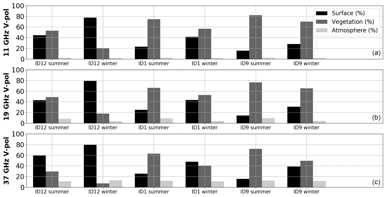
Figure 9Percentage of surface (black), vegetation (dark gray), and atmosphere (light gray) contributions to the simulated PMW signal at the top of the atmosphere (before DA) at the three frequencies 11 (a), 19 (b), and 37 GHz (c). ID12, ID1, and ID9 are Site 12 (fcover of 24.2 %), 1 (fcover of 63.7 %), and 9 (fcover of 84.0 %), respectively (see Table 2). Summer and winter periods are defined as periods when snowpack is observed or not.
An ensemble data assimilation (DA) scheme was implemented in a calibrated chain of models (Crocus/DMRT-ML, soil, vegetation, and atmosphere radiative transfer models) to improve SWE estimates by updating forcing data and snowpack states with the AMSR-2 satellite observations. The developed approach does not use any surface-based data and was tested over a boreal forest area in Quebec (eastern Canada). The proposed DA scheme is a particle filter with a resampled SIR algorithm, using an inflation technique of the R matrix to avoid degeneracy problems. The multilayer snowpack model, Crocus, coupled to the surface land model ISBA, was used to simulate the evolution of the snowpack. The DMRT-ML, the (ω-τopt) model, an atmospheric model, and the Wegmüller and Mätzler (1999) radiative transfer model were pre-calibrated to simulate the PMW contributions from the snowpack, the vegetation, and the soil, respectively, at the top of the atmosphere. The DA scheme was performed over 43 winters (12 sites from 2012 to 2016; Table 1), only in the presence of dry snow. Ice lenses were detected and integrated in the snowpack by using a thresholding approach on the polarization ratio at 11 GHz. The study shows the following.
-
TB TOAcan be well simulated with the developed chain of models. By calibrating soil and forest parameters (ω=0.07 and σs=0.2 cm), the annual TB TOA RMSE (all frequencies) is equal to 14.5 K from 2012 to 2016. This RMSE is similar to the overall RMSE estimated with the τsnow-calibrated DMRT-ML model driven by in situ measurements in an open area (19.9 K compared to surface-based radiometric measurements in Quebec; Larue et al., 2018).
-
The assimilation of TBs at 11, 19, and 37 GHz (V-pol) improves the SWE estimates compared to the assimilation of ΔTB 19−37 only (sensitive to snowpack depth) or to the assimilation of both ΔTB 19−37 and ΔTB 11−19. For three sites (with different fcover), the SWE ensemble RMSE of posterior estimates is reduced by 47 % over the whole winter compared to the SWE ensemble RMSE of prior estimates (open loop runs).
-
By using pre-calibrated ω and τsnow parameters in the DA scheme, the overall bias (for 43 winters) of the original SWECrocus simulations is significantly reduced by assimilating TBs at 11, 19, and 37 GHz (from 23.7 to 7.5 kg m−2). The bias on SWEmax is reduced by 12.2 kg m−2 (8 % of SWE measurements). The overall RPE goes from 22.1 % to 18.4 %, which is close to the range of accuracy needed for hydrological applications (SWE RPE <15 %). This accuracy is achieved with the TB assimilation for sites with an fcover below 75 %, but the DA deteriorates SWE simulations for sites with an fcover above 75 %. However, by using ω and τsnow as free variables, the DA significantly improves SWE simulations for sites with an fcover above 75 % (RPE =17.5 %).
Even with the difficulties associated with quantifying all the different factors that contribute to the PMW signal measured by satellite sensors in remote boreal areas (canopy, ice crust, frozen/unfrozen ground, presence of lakes, moisture in the snow, topography, etc.) (Kelly et al., 2003; Koenig and Forster, 2004), and even when vegetation contributions are 50 % of the PMW signal, the implementation of a DA scheme in a well-calibrated chain of models reduces SWE uncertainties without using any surface-based data. This assimilation scheme can be easily implemented in an operational system using real satellite-borne observations, despite the relatively significant computing time required. This research opens the way for global applications to obtain more accurate SWE estimates over large and remote areas where few meteorological weather stations are present.
The daily SWE data provided by Hydro-Québec are used for hydrological purposes and are not available to the public due to legal constraints on the data's availability. For the SWE and SD data, and field campaign measurements provided by the University of Sherbrooke, please contact the coauthor Alain Royer (Alain.Royer@USherbrooke.ca). Meteorological GEM data are freely available on the government of ECCC's website (Environment and Climate Change Canada) at https://weather.gc.ca/grib/grib2_reg_10km_e.html, last access: 10 October 2018). Other data used are listed in the references.
Online adjustment of covariance matrices in data assimilation is quite a common approach with the ensemble Kalman filter (Dee, 1995; Miyoshi, 2011; Brankart et al., 2010) but not with the particle filter. However, in many implementations of the particle filter, the measurement pdf is considered Gaussian, so the particle weights are computed using the observation error covariance matrix R. This matrix can therefore also be subject to adjustment in the context of the particle filter. Online adjustment can be and is often performed by tuning a simple inflation of the initial covariance matrix. This is the approach chosen here.
Noting , the innovation for particle i, the weight of this particle, is
where
An inflation of matrix R by a factor 1∕α (larger than 1) can be interpreted as an exponent α (smaller than 1) to wei. Because the weights wei are nonlinear functions of R, inflating R tends to flatten their distribution. Online adjustment consists in finding a value for α that flattens the distribution of weights to the point at which Nkeep particles are selected with certainty, Nkeep being a number to be prescribed. If the number Nkeep is fixed, when the resampling step is performed using Arakawa's procedure (Arakawa, 1997), the weight of the Nkeep−th particle to be selected, , must become equal to . Consequently,
or, written differently after taking the logarithm:
This equation for α is not solvable analytically. Instead, we find α after the convergence of the series:
The result of this adjustment is illustrated in Fig. A1. The blue dots show the first 20 weights of a sorted distribution for an ensemble of 50 particles strongly prone to degeneracy: only 4 particles have a weight larger than . The minimum number of particles to be selected is fixed to Nkeep=10. After the adjustment procedure, the identified inflation factor for matrix R is 3.6 (α=0.277), and the weight wekeep of the 10th particle is exactly equal to 0.02.
Obviously, this procedure is only used if the number of selected particles is below the Nkeep threshold with the initial weights.
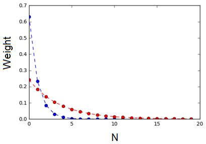
Figure A1Weight distribution of the first 20 weights of a sorted distribution for an ensemble of 50 particles: distribution before the adjustment (blue dotted points), showing a degeneracy problem, and distribution after the adjustment procedure (red dotted points), in which weight distribution is flattened and significant weights are distributed around Nkeep particles (10 particles for this example).
FL, AR, DS, and EC contributed to the conception and design of the work. All authors contributed to the acquisition, analysis, and interpretation of data. FL created new software used in the work. FL and AR wrote the manuscript, and all authors contributed to revisions of the manuscript.
The authors declare that they have no conflict of interest.
This article is part of the special issue “Integration of Earth observations and models for global water resource assessment”. It is not associated with a conference.
The authors would like to thank the data providers:
Hydro-Québec, Environment Canada (CMC-ECCC), and the University of Laval.
This project was supported by financial contributions from NSERC, Canada,
FRQ-NT and MITACS Quebec, and the CFQCU France–Quebec collaboration
program.
Edited by: Jaap Schellekens
Reviewed by: two anonymous referees
Andreadis, K. M. and Lettenmaier, D. P.: Implications of representing snowpack stratigraphy for the assimilation of passive microwave satellite observations, J. Hydrometeorology, 13, 1493–1506, https://doi.org/10.1175/JHM-D-11-056.1, 2012.
Arakawa, A.: Adjustment mechanisms in atmospheric motions, J. Meteor. Soc. Japan, Special issue of collected papers, 75, 155–179, 1997.
Arulampalam, M. S., Maskell, S., Gordon, N., and Clapp, T.: A tutorial on particle filters for online nonlinear/non-Gaussian Bayesian tracking, IEEE T. Signal Proces., 50, 174–188, 2002.
Brankart, J.-M., E. Cosme, C.-E. Testut, P. Brasseur, and J. Verron: Efficient Adaptive Error Parameterizations for Square Root or Ensemble Kalman Filters: Application to the Control of Ocean Mesoscale Signals, Mon. Weather Rev., 138, 932–950, 2010.
Brown, R. and Tapsoba, D.: Improved mapping of snow water equivalent over Quebec, 64th Eastern Snow Conference, St. John's, Newfoundland, Canada, 2007.
Brown, R. D., Brasnett, B., and Robinson, D.: Gridded North American monthly snow depth and snow water equivalent for GCM evaluation, Atmos. Ocean, 41, 1–14, https://doi.org/10.3137/ao.410101, 2003.
Brown, R., Tapsoba, D., and Derksen, C.: Evaluation of snow water equivalent datasets over the Saint-Maurice river basin region of southern Québec, Hydrol. Process., 32, 2748–2764, https://doi.org/10.1002/hyp.13221, 2018.
Brucker, L., Royer, A., Picard, G., Langlois, A., and Fily, M.: Hourly simulations of the microwave brightness temperature of seasonal snow in Quebec, Canada, using a coupled snow evolution-emission model, Remote Sens. Environ., 115, 1966–1977, 2011.
Brun, E., Martin, E., Simon, V., Gendre, C., and Coleou, C.: An energy and mass model of snow cover suitable for operational avalanche forecasting, J. Glaciol., 35, 333–342, 1989.
Brun, E., David, P., Sudul, M., and Brunot, G.: A numerical model to simulate snow cover stratigraphy for operational avalanche forecasting, J. Glaciol., 38, 13–22, 1992.
Carmagnola, C. M., Morin, S., Lafaysse, M., Domine, F., Lesaffre, B., Lejeune, Y., Picard, G., and Arnaud, L.: Implementation and evaluation of prognostic representations of the optical diameter of snow in the SURFEX/ISBA-Crocus detailed snowpack model, The Cryosphere, 8, 417–437, https://doi.org/10.5194/tc-8-417-2014, 2014.
Cavalieri, D. J., Gloersen, P., and Campbell, W. J.: Determination of sea ice parameters with the Nimbus 7 SMMR, J. Geophys. Res., 89, 5355–5369, 1984.
Chang, A. T. C., Foster, J. L., and Hall, D. K.: Nimbus-7 derived global snow cover parameters, Ann. Glaciol., 9, 39–44, 1987.
Chang, A. T. C., Foster, J. L., and Hall, D. K.: Effects of forest on the snow parameters derived from microwave measurements during the BOREAS winter field campaign, Hydrol. Process., 10, 1565–1574, 1996.
Charrois, L., Cosme, E., Dumont, M., Lafaysse, M., Morin, S., Libois, Q., and Picard, G.: On the assimilation of optical reflectances and snow depth observations into a detailed snowpack model, The Cryosphere, 10, 1021–1038, https://doi.org/10.5194/tc-10-1021-2016, 2016.
Choquette, Y., Lavigne, P., Nadeau, M., Ducharme, P., Martin, J. P., Houdayer, A., and Rogoza, J.: GMON, a new sensor for snow water equivalent via gamma monitoring, Proceedings Whistler 2008 International Snow Science Workshop, 21–27 September 2008, Whistler, B. C., 2008.
Côté, J., Gravel, S., Méthot, A., Patoine, A., Roch, M., and Staniforth, A.: The operational CMC-MRB Global Environmental Multiscale model: Part I – Design considerations and formulation, Mon. Weather Rev., 126, 1373–1395, 1998.
DeChant, C. and Moradkhani, H.: Radiance data assimilation for operational snow and streamflow forecasting, Adv. Water Res., 34, 351–364, 2011.
Decharme, B., Boone, A., Delire, C., and Noilhan, J.: Local evaluation of the Interaction between Soil Bio- sphere Atmosphere soil multilayer diffusion scheme using four pedotransfer functions, J. Geophys. Res., 116, D20, https://doi.org/10.1029/2011JD016002, 2011.
Dee, D. P.: On-line Estimation of Error Covariance Parameters for Atmospheric Data Assimilation, Mon. Weather Rev., 123, 1128–1145, 1995.
De Lannoy, G. J. M., Reichle, R., Houser, P., Arsenault, K., Verhoest, N., and Pauwels, V.: Satellite-Scale Snow Water Equivalent Assimilation into a High-Resolution Land Surface Model, J. Hydrometeorol., 11, 352–369, https://doi.org/10.1175/2009JHM1192.1, 2010.
De Lannoy, G. J. M., Reichle, R. H., Arsenault, K. R., Houser, P. R., Kumar, S., Verhoest, N. E. C., and Pauwels, V. R. N.: Multiscale assimilation of AMSR-E snow water equivalent and MODIS snow cover fraction observations in northern Colorado, Water Resour. Res., 48, W01522, https://doi.org/10.1029/2011WR010588, 2012.
De Sève, D., Bernier, M., Fortin, J. P., and Walker, A. E.: Preliminary analysis of the snow microwave radiometry using SSM/I passive microwave data: The case of the La Grande River watershed (Québec), Ann. Glaciol., 25, 353–361, 1997.
De Sève, D., Bernier, M., Fortin, J. P., and Walker, A.: Spatio-temporal analysis of microwave radiometry of snow cover with SSM/I data in a taïga area, Eastern Snow Conference, Fredericton, Canada, 200–205, 1999.
De Sève, D., Evora, N. D., and Tapsoba, D.: Comparison of three algorithms for estimating Snow Water Equivalent (SWE) over the La Grande River watershed using SSM/I data in the context of Hydro-Québec's hydraulic power management, Int. Geosci. Remote Se., IGARSS 23–28 July 2007, https://doi.org/10.1109/IGARSS.2007.4423791, 2007.
Derksen, C., Toose, P., Lemmetyinen, J., Pulliainen, J., Langlois, A., Rutter, N., and Fuller, M.: Evaluation of passive microwave brightness temperature simulations and snow water equivalent retrievals through a winter season, Remote Sens. Environ., 117, 236–248, 2012.
Derksen, C., Lemmetyinen, J., Toose, P., Silis, A., Pulliainen, J., and Sturm, M.: Physical properties of Arctic versus subarctic snow: Implications for high latitude passive microwave snow water equivalent retrievals, J. Geophys. Res.-Atmos., 119, 7254–7270, 2014.
Dobson, M. C., Ulaby, F. T., Hallikainen, M. T., and El-Rayes, M. A.: Microwave dielectric behavior of wet soil-part II: dielectric miximg models, IEEE T. Geosci. Remote, 1, 35–46, 1985.
Dolant, C., Langlois, A., Montpetit, B., Brucker, L., Roy, A., and Royer, A.: Development of a rain-on-snow detection algorithm using passive microwave radiometry, Hydrol. Process., 30, 3184–3196, https://doi.org/10.1002/hyp.10828, 2016.
Ducharme, P.: Estimation de l'équivalent en eau du couvert nival (Plan de projet étape 3), Technical report, Plate-forme Production, Hydro-Québec publication, Varennes, QC, Canada, 2003.
Durand, M. and Margulis, S.: Feasibility test of multi-frequency radiometric data assimilation to estimate snow water equivalent, J. Hydrometeorol., 7, 443–457, 2006.
Durand, M. and Margulis, S. A.: Correcting first-order errors in snow water equivalent estimates using a multifrequency, multiscale radiometric data assimilation scheme, J. Geophys. Res., 112, D13121, https://doi.org/10.1029/2006JD008067, 2007.
Durand, M., Kim, E. J., and Margulis, S. A.: Radiance assimilation shows promise for snowpack characterization, Geophys. Res. Lett., 36, L02503, https://doi.org/10.1029/2008GL035214, 2009.
Durand, M., Kim, E., Margulis, S., and Molotch, N.: A first-order characterization of errors from neglecting stratigraphy in forward and inverse passive microwave modeling of snow, IEEE Geosci. Remote Se., 8, 730–734, 2011.
Dutra, E., Kotlarski, S., Viterbo, P., Balsamo, G., Miranda, P. M. A., Schär, C., Bissolli, P., and Jonas, T.: Snow cover sensitivity to horizontal resolution, parameterizations and atmospheric forcing in a land surface model, J. Geophys. Res., 116, D21109, https://doi.org/10.1029/2011JD016061, 2011.
Foster, J., Sun, C., Walker, J., Kelly, R., Chang, A., Dong, J., and Powell, H.: Quantifying the uncertainty in passive microwave snow water equivalent observations, Remote Sens. Environ., 94, 187–203, 2005.
Franklin, S. E.: Terrain analysis from digital patterns in geomorphometry and Landsat MSS spectral response, Photogramm. Eng. Rem. S., 53, 59–65, 1987.
Gordon, N. J., Salmond, D. J., and Smith, A. F.: Novel approach to nonlinear/non-Gaussian Bayesian state estimation, IEEE Proc.-F, 140, 107–113, 1993.
Grant, J. P., Saleh, K., Wigneron, J.-P., Guglielmetti, M., Kerr, Y. H., Schwank, M., Skou, N., and Van de Griend, A.: Calibrationof the L-MEB model over a coniferous and a deciduous forest, IEEE Trans. Geosci. Remote Sens., 46, 808–818, https://doi.org/10.1109/TGRS.2007.914801, 2008.
Grant, A., Van de Griend, A., Schwank, M., and Wigneron, J.-P.: Observations and modeling of a pine forest floor at L-band, IEEE T. Geosci. Remote, 47, 2024–2034, https://doi.org/10.1109/TGRS.2008.2010252, 2009.
Hallikainen, M.: Retrieval of Snow Water Equivalent from Nimbus-7 SMMR Data: Effect of Land-Cover Categories and Weather Conditions, IEEE J. Oceanic Eng., OE-9, 372–376, https://doi.org/10.1109/JOE.1984.1145656, 1984.
Imaoka, K., Kachi, M., Kasahara, M., Nakagawa, K., and Oki, T.: Instrument performance and calibration of AMSR-E and AMSR2, International Archives of the Photogrammetry, Remote Sensing and Spatial Information Science, ISPRS, Kyoto, Japan, 2010.
Jordan, R. E.: A one-dimensional temperature model for a snow cover: Technical documentation for SNTHERM.89, Special Rep. 91-16, U.S. Army Cold Regions Research and Engineering Laboratory, Hanover, NH, 49 pp., 1991.
Kelly, R., Chang, A. T. C., Tsang, L., and Foster, J.: A prototypeAMSR-E global snowarea and snow depth algorithm, IEEE Trans. Geosci. Rem. Sens, 41, 23, 2003.
Kelly, R., Chang, A. T. C., Tsang, L., and Foster, J.: A prototype AMSR-E global snow area and snow depth algorithm, IEEE T. Gesoci. Remote, 41, 230–242, 2010.
Klehmet, K., Geyer, B., and Rockel, B.: A regional climate model hindcast for Siberia: analysis of snow water equivalent, The Cryosphere, 7, 1017–1034, https://doi.org/10.5194/tc-7-1017-2013, 2013.
Koenig, L. S. and Forster, R. R.: Evaluation of passive microwave snow water equivalent algorithms in the depth-hoar dominated snowpack of the Kuparuk River Watershed, Alaska, USA, Remote Sens. Environ., 93, 511–527, 2004.
Kwon, Y., Yang, Z.-L., Zhao, L., Hoar, T. J., Toure, A. M., and Rodell, M.: Estimating snow water storage in North America using CLM4, DART, and snow radiance data assimilation, J. Hydrometeorol., 17, 2853–2874, 2016.
Kwon, Y., Yang, Z.-L., Hoar, T. J., and Toure, A. M.: Improving the Radiance Assimilation Performance in Estimating Snow Water Storage across Snow and Land-Cover Types in North America, J. Hydrometeorol., 18, 651–668, 2017.
Lafaysse, M., Cluzet, B., Dumont, M., Lejeune, Y., Vionnet, V., and Morin, S.: A multiphysical ensemble system of numerical snow modelling, The Cryosphere, 11, 1173–1198, https://doi.org/10.5194/tc-11-1173-2017, 2017.
Langlois, A., Royer, A., Derksen, C., Montpetit, B., Dupont, F., and Goïta, K.: Coupling of the snow thermodynamic model SNOWPACK with the Microwave Emission Model for Layered Snowpacks (MEMLS) for subarctic and arctic Snow Water Equivalent retrievals, Water Resour. Res., 48, W12524, https://doi.org/10.1029/2012WR012133, 2012.
Langlois, A. et al.: Detection of rain-on-snow (ROS) events and ice layer formation using passive microwave radiometry: a context for Peary caribou habitat in the Canadian Arctic, Remote Sens. Environ., 189, 84–95, https://doi.org/10.1109/TGRS.1982.4307521, 2017.
Larue, F., Royer, A., De Sève, D., Langlois, A., Roy, A., and Brucker, L.: Validation of GlobSnow-2 snow water equivalent over Eastern Canada, Remote Sens. Environ., 194, 264–277, https://doi.org/10.1016/j.rse.2017.03.027, 2017.
Larue, F., Royer, A., De Sève, D., Roy, A., Picard, G., Vionnet, V., and Cosme, E.: Simulation and assimilation of passive microwave data using a snowpack model coupled to a calibrated radiative transfer model over northeastern Canada, Water Resour. Res., 54, 4823–4848, https://doi.org/10.1029/2017WR022132, 2018.
Lehning, M., Bartelt, P., Brown, R. L., and Fierz, C.: A physical SNOWPACK model for the Swiss avalanche warning; Part III: meteorological forcing, thin layer formation and evaluation, Cold Reg. Sci. Technol., 35, 169–184, 2002.
Leppänen, L., Kontu, A., Vehviläinen, J., Lemmetyinen, J., and Pulliainen, J.: Comparison of traditional and optical grain size field measurements with SNOWPACK simulations in a taiga environment, J. Glaciol., 61, 151–162, 2015.
Liebe, H.: MPM – an atmospheric millimeter-wave propagation model, Int. J. Infrared Milli., 10, 631–650, 1989.
Luojus, K., Pulliainen, J., Takala, M., Lemmetyinen, J., Smolander, T., and Derksen, C.: The GlobSnow Snow Water Equivalent Product, 22 July 2014, SnowPEX ISSPI-1, College Park, Maryland, USA, 2014.
Masson, V., Le Moigne, P., Martin, E., Faroux, S., Alias, A., Alkama, R., Belamari, S., Barbu, A., Boone, A., Bouyssel, F., Brousseau, P., Brun, E., Calvet, J.-C., Carrer, D., Decharme, B., Delire, C., Donier, S., Essaouini, K., Gibelin, A.-L., Giordani, H., Habets, F., Jidane, M., Kerdraon, G., Kourzeneva, E., Lafaysse, M., Lafont, S., Lebeaupin Brossier, C., Lemonsu, A., Mahfouf, J.-F., Marguinaud, P., Mokhtari, M., Morin, S., Pigeon, G., Salgado, R., Seity, Y., Taillefer, F., Tanguy, G., Tulet, P., Vincendon, B., Vionnet, V., and Voldoire, A.: The SURFEXv7.2 land and ocean surface platform for coupled or offline simulation of earth surface variables and fluxes, Geosci. Model Dev., 6, 929–960, https://doi.org/10.5194/gmd-6-929-2013, 2013.
Mätzler, C.: Applications of the interaction of microwaveswith the natural snow cover, Remote Sens. Rev., 2, 259–387, https://doi.org/10.1080/02757258709532086, 1987.
Mätzler, C.: Passive microwave signatures of landscapes in winter, Meteorol. Atmos. Phys., 54, 241–260, 1994.
Mätzler, C., Schanda, E., and Good, W.: Towards the definition of optimum sensor specifications for microwave remote sensing of snow, IEEE T. Geosci. Remote, GE-20, 57–66, 1982.
Meissner, T. and Wentz, F.: Intercalibration of AMSR-E and WINDSAT brightness temperature measurements over land scenes, presented at the 11th Specialist Meeting on Microwave Radiometry and Remote Sensing of the Environment (MicroRad 2010), 1–4 March 2010, Washington, DC, USA, 2010.
Mo, T., Choudhury, B. J., Schmugge, T. J., Wang, J. R., and Jackson, T. J.: A model for microwave emission from vegetation-covered fields, J. Geophys. Res., 87, 11 229–11 237, 1982.
Molotch, N. P. and Bales, R. C.: Scaling snow observations from the point to the grid element: Implications for observation network design, Water Resour. Res., 41, W11421, https://doi.org/10.1029/2005WR004229, 2005.
Montpetit, B., Royer, A., Roy, A., Langlois, A., and Derksen, D.: Snow microwave emission modeling of ice lenses within a snowpack using the microwave emission model for layered snowpacks, IEEE T. Geosci. Remote, 51, 4705–4717, https://doi.org/10.1109/TGRS.2013.2250509, 2013.
Montpetit, B., Royer, A., Roy, A., and Langlois, A.: In-situ passive microwave parameterization of sub-arctic frozen organic soils, Remote Sens. Environ., 205, 112–118, 2018.
Myneni, R. B., Hoffman, S., Knyazikhin, Y., Privette, J. L., Glassy, J., Tian, Y., Wang, Y., Song, X., Zhang, Y., Smith, G. R., Lotsch, A., Friedl, M., Morisette, J. T., Votava, P., Nemani, R. R., and Running, S. W.: Global products of vegetation leaf area and fraction absorbed PAR from year one of MODIS data, Remote Sens. Environ., 83, 214–231, 2002.
Miyoshi, T.: The Gaussian Approach to Adaptive Covariance Inflation and Its Implementation with the Local Ensemble Transform Kalman Filter, Mon. Weather Rev., 139, 1519–1535, 2011.
Pampaloni, P. and Paloscia, S.: Microwave emission and plant water content: A comparison between field measurements and theory, IEEE T. Geosci. Remote, GE-24, 900–905, https://doi.org/10.1109/TGRS.1986.289705, 1986.
Pellarin, T., Kerr, Y. H., and Wigneron, J. P.: Global simulation of brightness temperatures at 6.6 and 10.7 GHz over land based on SMMR data set analysis, IEEE T. Geosci. Remote, 44, 2492–2505, 2006.
Picard, G., Brucker, L., Roy, A., Dupont, F., Fily, M., Royer, A., and Harlow, C.: Simulation of the microwave emission of multi-layered snowpacks using the Dense Media Radiative transfer theory: the DMRT-ML model, Geosci. Model Dev., 6, 1061–1078, https://doi.org/10.5194/gmd-6-1061-2013, 2013.
Pietroniro, A. and Leconte, R.: A review of Canadian Remote Sensing and Hydrology 1999–2003, Hydrol. Process., 19, 285–301, 2005.
Pulliainen, J. T., Grandel, J., and Hallikainen, M. T.: HUT snow emission model and its applicability to snow water equivalent retrieval, IEEE T. Geosci. Remote, 37, 1378—1390, 1999.
Quéno, L., Vionnet, V., Dombrowski-Etchevers, I., Lafaysse, M., Dumont, M., and Karbou, F.: Snowpack modelling in the Pyrenees driven by kilometric-resolution meteorological forecasts, The Cryosphere, 10, 1571–1589, https://doi.org/10.5194/tc-10-1571-2016, 2016.
Raleigh, M. S., Lundquist, J. D., and Clark, M. P.: Exploring the impact of forcing error characteristics on physically based snow simulations within a global sensitivity analysis framework, Hydrol. Earth Syst. Sci., 19, 3153–3179, https://doi.org/10.5194/hess-19-3153-2015, 2015.
Rott, H., Yueh, S. H., Cline, D. W., Duguay, C., Essery, R., Haas, C., Hélière, F., Kern, M. G., Malnes, E., Nagler, T., Pulliainen, J., Rebhan, H., and Thompson, A.: Cold regions hydrology high-resolution observatory for Snow and Cold Land Processes, Proc. IEEE,, 98, 752–765, https://doi.org/10.1109/JPROC.2009.2038947, 2010.
Roy, A., Royer, A., and Turcotte, R.: Analyse de l'identification de la fonte de neige printanière avec QuickSCAT dans le Sud du Québec, Canada, Can. J. Remote Sens., 36, 89–98, 2010.
Roy, A., Royer, A., Wigneron, J.-P., Langlois, A., Bergeron, J., and Cliche, P.: A simple parameterization for a boreal forest radiative transfer model at microwave frequencies, Remote Sens. Environ., 124, 371–383, 2012.
Roy, A., Picard, G., Royer, A., Montpetit, B., Dupont, F., Langlois, A., Derksen, C., and Champollion, N.: Brightness Temperature Simulations of the Canadian Seasonal Snowpack Driven by Measurements of the Snow Specific Surface Area, IEEE T. Geosci. Remote., 51, 4692–4704, 2013.
Roy, A., Royer, A., and Hall, R.: Relationship between forest microwave transmissivity and structural parameters for Canadian boreal forest, IEEE Geosci. Remote S., 11, 1802–1806, 2014.
Roy, A., Royer, A., St-Jean-Rondeau, O., Montpetit, B., Picard, G., Mavrovic, A., Marchand, N., and Langlois, A.: Microwave snow emission modeling uncertainties in boreal and subarctic environments, The Cryosphere, 10, 623–638, https://doi.org/10.5194/tc-10-623-2016, 2016.
Royer, A., Roy, A., Montpetit, B., Saint-Jean-Rondeau, O., Picard, G., Brucker, L., and Langlois, A.: Comparison of commonly-used microwave radiative transfer models for snow remote sensing, Remote Sens. Environ., 190, 247–259, 2017.
Sandells, M., Essery, R., Rutter, N., Wake, L., Leppänen, L., and Lemmetyinen, J.: Microstructure representation of snow in coupled snowpack and microwave emission models, The Cryosphere, 11, 229–246, https://doi.org/10.5194/tc-11-229-2017, 2017.
Sun, C., Walker, J. P., and Houser, P. R.: A methodology for snow data assimilation in a land surface model, J. Geophys. Res., 109, D08108, https://doi.org/10.1029/2003JD003765, 2004.
Takala, M., Luojus, K., Pulliainen, J., Derksen, C., Lemmetyinen, J., Kärnä, J.-P., Koskinen, J., and Bojkov, B.: Estimating northern hemisphere snow water equivalent for climate research through assimilation of space-borne radiometer data and ground-based measurements, Remote Sens. Environ., 115, 3517–3529, 2011.
Tapsoba, D., Fortin, V., Anctil, F., Haché, M.: Apport de la technique du krigeage avec dérive externe pour une cartographie raisonnée de l'équivalent en eau de la neige: application aux bassins de la rivière Gatineau, Can. J. Civ. Eng., 32, 289–297, 2005.
Tapsoba, D., Fortin, V., Anctil, F., and Haché, M.: Apport de la technique du krigeage avec dérive externe pour une cartographie raisonnée de l'équivalent en eau de la neige: Application aux bassins de la rivière Gatineau, Can. J. Civil Eng., 32, 289–297, 2009.
Tedesco, M. and Narvekar, P. S.: Assessment of the NASA AMSR-E SWE product, IEEE J. Sel. Top. Appl., 3, 141–159, 2010.
Tedesco, M., Kelly, R., Foster, J. L., and Chang, A. T. C.: AMSR-E/Aqua Daily L3 Global Snow Water Equivalent EASE-Grids, Version 2, NASA National Snow and Ice data center Distributed Active Archive Center, Boulder, Colorado, USA, https://doi.org/10.5067/AMSR-E/AE_DYSNO.002, 2004.
Touré, A., Goïta, K., Royer, A., Kim, E., Durand, M., Margulis, S. A., and Huizhong, Lu: A Case Study of Using a Multi-Layered Thermo-Dynamical Snow Model for Radiance Assimilation, IEEE T. Geosci. Remote, 49, 2828–2837, 2011.
Tsang, L. and Kong, J. A.: Scattering of Electromagnetic Waves, vol. 3, Advanced Topics, Wiley Intersci., Hoboken, N. J., 2001.
Tsang, L., Ding, K. H., and Wen, B.: Dense Media Radiative Transfer Theory for Dense Discrete Random Media with Particles of Multiple Sizes and Permitivities, Pr. Electromagn. Res., 6, 181–230, 1992.
Turcotte, R., Fortier-Filion, T.-C., Fortin, V., Roy, A., and Royer, A.: Simulation hydrologiques des derniers jours de la crue du printemps: le problème de la neige manquante, Hydrolog. Sci. J., 55, 872–882, 2010.
Vachon, F.: Estimation de l'équivalent en eau de la neige en milieu subarctique du Québec par télédétection micro-ondes passives, Mémoire de thèse, Université de Sherbrooke, Sherbrooke, Canada, Mai 2009.
Van Leeuwen, P. J.: Particle filtering in geophysical systems, Mon. Weather Rev., 137, 4089–4114, https://doi.org/10.1175/2009MWR2835.1, 2009.
Van Leeuwen, P. J.: Particle filters for the geosciences, Advanced Data Assimilation for Geosciences: Lecture Notes of the Les Houches School of Physics: Special Issue, June 2012, in: Advanced Data Assimilation for Geosciences, 291–318, https://doi.org/10.1093/acprof:oso/9780198723844.003.0013, 2014.
Vionnet, V., Brun, E., Morin, S., Boone, A., Faroux, S., Le Moigne, P., Martin, E., and Willemet, J.-M.: The detailed snowpack scheme Crocus and its implementation in SURFEX v7.2, Geosci. Model Dev., 5, 773–791, https://doi.org/10.5194/gmd-5-773-2012, 2012.
Wang, N., Liu, C., Ferraro, R., Wolff, D., Zipser, E., and Kummerow, C.: TRMM 2A12 land precipitation product-status and future plans, J. Met. Soc. of Japan, 87, 237–253, 2009.
Wegmüller, U. and Mätzler, C.: Rough bare soil reflectivity model, IEEE T. Geosci. Remote, 37, 1391–1395, 1999.
Xu, X., Li, J., and Tolsonv, B. A.: Progress in integrating remote sensing data and hydrologic modeling, Prog. Phys. Geog., 38, https://doi.org/10.1177/0309133314536583, 2014.