the Creative Commons Attribution 4.0 License.
the Creative Commons Attribution 4.0 License.
 | 05 Oct 2018
Design water demand of irrigation for a large region using a high-dimensional Gaussian copula
Yiliang Du
Vijay P. Singh
Xiaohong Chen
Kairong Lin
Haiou Wu
Spatial and frequency distributions of precipitation should be considered in determining design water demand of irrigation for a large region. In Guangdong Province, South China, as a study case, an eight-dimensional joint distribution of precipitation for agricultural sub-regions was developed. A design procedure for water demand of irrigation for a given frequency of precipitation of the entire region was proposed. Water demands of irrigation in the entire region and its sub-regions using three design methods, i.e., equalized frequency (EF), typical year (TY) and most-likely weight function (MLW), were compared. Results demonstrated that the Gaussian copula efficiently fitted the high-dimensional joint distribution of eight sub-regional precipitation values. The Kendall frequency was better than the conventional joint frequency to analyze the linkage between the frequency of precipitation of the entire region and individual sub-regions. For given frequencies of precipitation of the entire region, design water demands of irrigation of the entire region among the MLW, EF and TY methods slightly differed, but those of individual sub-regions of the MLW and TY methods fluctuated around the demand lines of the EF method. The alterations of design water demand in sub-regions were more complicated than those in the entire region. The design procedure using the MLW method in association with a high-dimensional copula, which simulated individual univariate distributions, captured their dependences for multi-variables, and built a linkage between regional frequency and sub-regional frequency of precipitation, is recommended for design water demand of irrigation for a large region.
- Article
(1424 KB) - Full-text XML
- BibTeX
- EndNote


Water demand of irrigation in a region is associated with exploitation and utilization of land and water resources, such as farm area, cultivation pattern, category of crops, canal technology, etc., and is also impacted by natural factors, for example precipitation volume and soil properties (Tarjuelo et al., 2005; Griffin, 2006; Leenhardt et al., 2004, 2011; Wriedt et al., 2009; Davidson and Hellegers, 2011). Among the many factors, precipitation, which is regarded as stochastic, is an uncertain factor influencing irrigation (Wisser et al., 2008; Thomas, 2008; Cai et al., 2011; Meza et al., 2012). In general, the more the precipitation, the less the water demand of irrigation, and vice versa. In practical regional water resources planning, water demands of irrigation are estimated in association with various frequencies of regional precipitation (Gohari et al., 2013).
For design water demand in a large region, it is important that the heterogeneity of those factors in geographical space is considered (Lankford, 2010; Leenhardt et al., 2011). Hence, water demand should generally be analyzed in separate sub-regions in which the factors are homogenous, and can eventually be summed up. However, for a given precipitation frequency of the entire region in the design water demand of irrigation, the difficulty is how to obtain a reasonable combination of precipitation frequencies of multiple sub-regions, even though other factors influencing irrigation have previously been demonstrated in water resources planning.
A method, named typical year (TY), has been used for design water demand of irrigation in China (Cai et al., 2001). A combination of observed sub-regional precipitation in a certain year in which the precipitation frequency for the entire region weighted by individual sub-regions was the nearest to the given frequency, was selected and was zoomed in or out. Due to the limited observed samples, the representation of the typical year has been questionable. In actuality, the frequency of regional precipitation in a large region corresponds to various combinations of sub-regional frequencies.
Moreover, design water demand of irrigation in a large region not only presents the stochastic characteristic of precipitation in the entire region and its sub-regions, but also addresses the relationship between sub-regional precipitation and heterogeneity. The multi-variable statistical simulation and joint design theory can be considered to improve the selection of an appropriate combination. Due to the multivariate dependence and the flexibility of unbounded marginal distributions, copula functions have been widely applied in the simulation and design of hydrological multi-variables, e.g., extreme properties of heavy precipitation (Zhang et al., 2011, 2013; Abdul Rauf and Zeephongsekul, 2014), floods (Zhang and Singh, 2006; Chowdhary et al., 2011; Zhang et al., 2015a) and droughts (Ganguli and Reddy, 2014; Zhang et al., 2015b; Tu et al., 2016). In recent years, they have been used to analyze floods or droughts encountered in multiple hydrological regions in China (Yan et al., 2010a; Xie et al., 2012; Tu et al., 2017b). These studies on multivariate hydrology mostly focused on bivariate and trivariate issues, but less on higher dimensional hydrological statistical analyses (Chen et al., 2015). A high-dimensional meta-Gaussian copula beyond three variables has been applied in other fields, e.g., economic analysis (Aussenegg and Cech, 2012; Creal and Tsay, 2015).
As a multidimensional copula and its marginal distributions are determined according to observed samples, the joint frequency and probability density for any combination of precipitation frequencies of sub-regions can be calculated. In a practical design combination, a large quantity of combinations can be randomly generated using the Monte Carlo method on the basis of the determined copula. It is clear that a given joint frequency corresponds to quite a number of combinations. In order to select one from various combinations, a simple method, based on the equalized frequency (EF) method, which refers to all marginal frequencies being identical, is used for design flood peak and volume (Liu et al., 2015).
Another improved method is that the combination can be exclusively determined by using the most-likely weight function (MLW) in association with the products of joint and marginal probability densities (Salvadori et al., 2011). The most-likely weight design method has been applied for the design combination of hydrological multivariables, such as flood and drought properties (Gräler et al., 2013; Zhang et al., 2015c), flood and tide or heavy precipitation and tide in coastal rivers (Corbella and Stretch, 2012; Lian et al., 2013; Zheng et al., 2013; Tu et al., 2017a), and the precipitation or streamflow of multiple regions (Yan et al., 2010b).
Furthermore, in practical water resources planning, the main concern is that water demand of irrigation of the entire region and that of sub-regions are designed for a given frequency of precipitation for the entire region, not for a given joint frequency of precipitation of sub-regions. The relationship between regional frequency and joint frequency of precipitation is also required to be investigated in determining design water demand of irrigation in a large region.
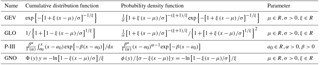
Table 1Theoretical cumulative distribution and probability density function of three parameter univariate distribution.
This paper considered water demand of irrigation of paddies in Guangdong Province, South China, as a case study of a large region. Annual precipitation data of eight agricultural sub-regions and their net quotas of irrigation in association with precipitation frequency were used. A high-dimensional meta-Gaussian copula and several conventional univariate distributions were applied to fit the joint and marginal distributions of sub-regional precipitation, respectively. Combinations of cumulative frequency for sub-regional precipitation were generated by using the Monte Carlo simulation method on the basis of the determined copula. The link between the joint frequency of sub-regional precipitation and the frequency of precipitation of the entire region was established. The methods, i.e., typical year, equalized frequency, and the most-likely weight function, were used for design combinations of sub-regional precipitation for given frequencies of precipitation of the entire region. Water demand of irrigation of the entire region and individual sub-regions among design methods was compared in order to improve design water demand of irrigation in a large region.
2.1 Water demand of irrigation of paddy
In a paddy field, water demand of irrigation per unit area, i.e., the net quota of irrigation, is determined by various factors, such as crop and soil types, cultivation pattern and precipitation process, etc. In regional planning of water resources, as other factors are demonstrated in advance, the net quota of irrigation mainly changes with annual precipitation due to the stochastic property of precipitation. In practice, the net quota of irrigation per unit area q(u) in association with the frequency of precipitation is determined via field experiments. Then, for a given frequency of annual precipitation, u, water demand of irrigation, W(u), which refers to water withdrawn from river or other water sources engineering, can be calculated as
where A and q(u) refer to the paddy area and the net quota of irrigation, respectively, and η is the utilization coefficient of irrigation, which refers to the ratio of net water supply in the field to water withdrawn from river or other water sources engineering.
In a large region, for example Guangdong Province, China, the differences of annual precipitation and the net quota of irrigation among individual agricultural regions are required to be considered. Then, for a given regional frequency of annual precipitation, u0, for a large region with sub-regions, water demand of irrigation, W(u0), can be deduced as follows:
where Ai refers to the irrigation area of the ith sub-region and qi(ui) is the net quota of irrigation per unit area at the frequency of precipitation of the ith sub-region, ui.
Therefore, the key point to design water demand of irrigation for a given precipitation frequency of the entire region, u0, is how to determine a combination of sub-regional precipitation frequencies, .
2.2 Annual precipitation distribution
If a large region consists of d sub-regions, let Xi be the series of annual precipitation in which and refer to sub-region d and n years, respectively. The theoretical cumulative distribution of annual precipitation in a sub-region, , can be fitted by several conventional three parameter univariate distributions, which have been widely used in hydrology, such as generalized extreme value (GEV), generalized logistic (GLO), Pearson III (P-III) and generalized normal (GNO). Their cumulative distribution and probability density functions are presented in Table 1.
The Kolmogorov–Smirnov (K–S) statistic, D, for the goodness-of-fit test of annual precipitation distribution of a sub-region was computed as (Dobric and Schmid, 2007; Massey, 2012; Tu et al., 2016)
The parameters of all recommended univariate distributions were estimated by the L-moment method. The critical values at the significance level of 0.05 for the goodness-of-fit test of all distributions were obtained by the Monte Carlo method with 5000 or more simulations. If the K–S statistic, D, which was computed from the samples, was less than the corresponding critical value, the tested distribution was accepted. The optimal distribution was selected from the accepted distributions by comparing their root-mean-square error (RMSE) and Akaike information criterion (AIC) values. In addition, empirical and theoretical distributions were compared to evaluate the goodness of fit of the observed samples of precipitation. In hydrological practice, the empirical distribution functions are defined and transformed by Gringorten (1963).
Subsequently, based on the areal weight method, the annual precipitation in the entire region, X0(j), was calculated as
Where αi refers to the areal ratio of the ith sub-region to the entire region. Then, the theoretical distribution of annual precipitation for the entire region, , can also be fitted by using the above recommended univariate distributions and the K-S test method.
2.3 Conventional design methods
2.3.1 Typical year method (TY)
In practical design, water demand of irrigation for a large region, a combination of observed sub-regional precipitation in a certain year, in which the precipitation of the entire region weighted by individual sub-regions is the nearest to that of a given frequency for the entire region, has been the only selection (Cai et al., 2001). The selected year was called the typical year corresponding to the given frequency of precipitation. Let be a given cumulative distribution frequency (CDF) of precipitation of the entire region. Then, the corresponding precipitation can be calculated by using the inverse function of the frequency distribution as follows:
Further, the relative alteration, , of the observed precipitation in each year compared to the precipitation of the given frequency, was defined as
Then,
where J is the selected rank of a certain year, which corresponds to the typical year for the given frequency .
In addition, due to the limited length of annual precipitation observations, the relative alteration R(J) of the typical selected year might be large. Namely, annual precipitation of the entire region weighted by sub-regional precipitation in a typical selected year, in terms of magnitude, may differ from that of the given frequency. Therefore, a scaling method was applied to zoom in or out for the sub-regional precipitation in the typical selected year as follows:
where β is a scale coefficient and Xi(J) and refer to the ith sub-regional precipitation before and after zooming in or out, respectively.
For a given precipitation frequency of the entire region, , individual sub-regional frequencies, , can eventually be deduced by their frequency distributions as follows:
2.3.2 Equalized frequency method (EF)
In order to get a combination of sub-regional frequencies for a given precipitation frequency of the entire region, the equalized frequency method (Liu et al., 2015) is also used for downscaling precipitation for a large region. As the name implies, the EF assumes that the frequencies of sub-regional precipitation are identical. That is, for a given precipitation frequency , let , and then can be found as follows:
where and refer to the precipitation in the entire region and sub-regions calculated by using the inverse function of individual frequency distributions, respectively. In practical design, the sub-regional frequency is determined by applying the method of successive search approximation within an available range.
2.4 Joint design based on copula function
2.4.1 Multidimensional joint distribution
For a large region, the difference of precipitation between any two sub-regions is associated with geographical location. Though annual precipitation in any sub-region is regarded as stochastic, there exists dependence between two sub-regions, in particular for adjacent sub-regions due to similar geographic and climate conditions. Herein, a multidimensional copula function was used for modeling the joint distribution of sub-regional precipitation. Assume that annual precipitation of each sub-region, , is a continuous random variable with a d-dimensional joint distribution and individual marginal distribution functions . Then, on the basis of the Sklar theorem (Nelsen, 2006), the joint distribution, , can be defined as
where is the d-dimensional copula function which is the joint distribution function of standard uniform random variables, and , refer to individual CDFs of sub-regional precipitation.
The copula function, which accommodates different marginal distributions of individual variables and captures their dependence, has been widely applied in multivariate hydrology. More details on the theoretical properties of various copula families can be found in Nelsen (2006). Owing to its flexibility, accessibility and simple copula parameters in association with a correlation coefficient matrix, a d-dimensional meta-Gaussian copula was selected for modeling the joint distribution of multiple sub-regional precipitations. Its theoretical cumulative distribution function, , and density function, , were deduced as follows (Genest et al., 2007):
where
where , in which refers to the inverse function of the standard normal distribution. and are the matrices of variables in the integrand. The correlation coefficient matrix Σ was expressed as
where, refers to the correlation coefficient between any two sub-regional precipitations.
For the goodness-of-fit test of multi-dimensional meta-Gaussian copula, the Cramér–von Mises test statistic on the basis of the Rosenblatt transform was used (Rosenblatt, 1952; Genest et al., 2009). For the joint distribution of sub-regional precipitation with a d dimension, the goodness-of-fit test statistics, , were formulated as
where , refers to the pseudo-observations of individual sub-regional precipitation. Let Ei=u1, and be assigned as (Rosenblatt, 1952; Dobric and Schmid, 2007)
A parametric bootstrap procedure for , deduced from the literature, is addressed in Appendix D (Genest et al., 2009). In multivariate practice, the joint empirical distribution functions are defined (Dobric and Schmid, 2007; Genest et al., 2009; Tu et al., 2016) and transformed by Gringorten (1963).
In addition, the Kendall function, which is a univariate expression of multivariate information (Genest and Rivest, 1993; Barbe et al., 1996; Salvadori et al., 2011, 2013), has been shown to be an appropriate tool for calculating the copula-based joint frequency of multivariate events (Nappo and Spizzichino, 2009; Salvadori et al., 2011) and is widely applied in discussing the joint probability or return period of hydrological multivariables (Salvadori and Michele, 2004; Michele et al., 2013). The Kendall CDF, , which was transformed from the joint CDF of eight sub-regional precipitation and was used in comparing it with the frequency of entire regional precipitation, was estimated as
where is the probability level and n refers to the length of observed or simulated samples. The function I(⋅) is an indicator function, which is equal to 1 when the enclosed expression is true, and 0 otherwise.
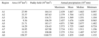
Table 2Area, paddy field and precipitation of the sub-regions and entire region. The A0 region refers to the entire region of Guangdong Province.
2.4.2 Most-likely weight function (MLW)
In multivariate design practice, using sample data of annual precipitation of all sub-regions, the univariate distribution of the entire region, joint and marginal distributions of sub-regions, and parameters of all distributions can be determined by the recommended univariate models and Gaussian copula. The Monte Carlo method can be used to simulate new combinations of CDFs of precipitation using the determined distributions and parameters. Then, the CDFs of precipitation of the entire region corresponding to each combination of sub-regional CDFs can be achieved. However, there are a large number of combinations which lead to the CDFs of the entire region, which can be almost identical within a predefined small difference. That is, a given CDF of precipitation of the entire region can correspond to many combinations of sub-regional CDFs with enough further simulations. The design realization using the most-likely weight function was proposed by Salvadori et al. (2011) as follows:
where is eventually selected as the design combination of CDFs of sub-regional precipitation for a given CDF of the entire region, . refers to the product of joint probability densities, , and their individual marginal probability densities, . Therefore, the procedure for design combination of sub-regional precipitation for a given CDF of the entire region was as follows.
-
The joint and marginal distributions and parameters of sub-regional precipitation were determined by the goodness of fit of the recommended d-dimensional meta-Gaussian copula and univariate distributions for the observed samples.
-
Using the Monte Carlo method according to the determined d-dimensional joint distribution, large quantities of combinations of CDFs of sub-regional precipitation, , with the number of simulations, m, were generated, and the corresponding combinations of sub-regional precipitation, , and precipitation and CDFs of the entire region, and , were calculated.
-
For a given CDF of precipitation of the entire region, , the allowable relative error, was defined as
where Re refers to the threshold value of allowable relative error. Then, in the simulated u0(j), those which satisfied Eq. (22) were selected. That is, with the length of l were found to satisfy and the selected combinations, and , corresponded to the given .
-
For all selected combinations, the products of the probability densities, , on the basis of the joint probability densities, and marginal , respectively, were calculated, and with the maxima of the product from was the design combination for the given CDF of precipitation of the entire region, .

In addition, in order to better present the relationship of the Kendall CDF of sub-regional precipitation and the CDF of precipitation of the entire region, a confidence interval (CI) was defined by the distance which deviated from the diagonal (Serinaldi, 2013; Volpi and Fiori, 2014) and transformed herein by the normal distribution. The CI with a probability of 1−α was involved.
The Guangdong Province as a study case is located in South China with a land area of 158.57×10³ km2 (illustrated in Fig. 1). The entire region mostly belongs to the monsoon climate zone, varying from the tropic to southern sub-tropic. Annual precipitation is abundant, but uneven in terms of spatial and temporal distribution. Since China's reform and opening up in the late 1970s, the water demand of the province has been increasing with the rapid development of the regional socio-economy. In 2015, the total water consumption of the province accounted for 44.31 billion m3, in which approximately one-half was for irrigation.
According to the report of the Irrigation Quota of Guangdong Province, the entire region marked by A0, in terms of agriculture on the basis of climate, soil type, cropping system and other management measures, was zoned into eight sub-regions marked by A1–A8 in Fig. 1. Areal data of sub-regions and their paddy fields were used (see Table 2). Annual precipitation data of eight sub-regions for the period of 1953–2013, in terms of multi-site average, were transformed from 25 hydro-meteorological stations.
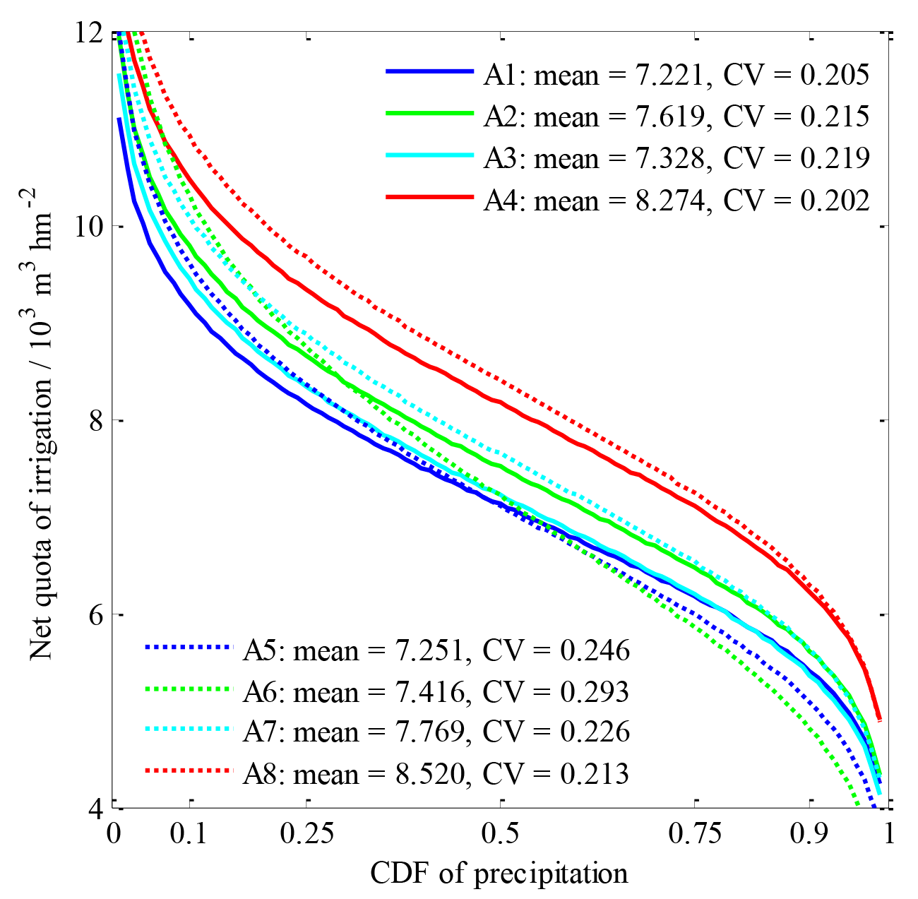
The net quotas of irrigation of individual sub-regions in association with precipitation frequency resulted from the previous field experiments of irrigation in the late twentieth century. According to the distribution and statistical properties on the basis of field experiments in a research report entitled Annual irrigation Quota in Guangdong Province (1999), the net quotas of irrigation per unit area in the paddy fields of individual sub-regions in association with the precipitation frequency are illustrated in Fig. 2. They ranged from 7221 to 8520 m3 hm−2 in terms of annual average with coefficients of variation of 0.205–0.293, and precipitation was regarded to follow the Pearson III distribution whose three parameters were transformed using the given mean values and coefficients of variation marked in Fig. 2.
The utilization coefficient of irrigation of Guangdong Province has been at a low level, which approximately accounted for 0.46 in terms of average value in 2000 according to the Water Resources Comprehensive Planning of Guangdong Province. In order to respond to tough national water management measures of China, the utilization coefficient is expected to be no less than 0.51 by 2020 in the Tough Water Management Assessing Performance of Guangdong Province. Therefore, the utilization coefficients of eight agricultural sub-regions were uniformly predefined as a fixed value of 0.51 in this paper.
4.1 Univariate properties and distribution of precipitation
Annual precipitation in the entire region and individual sub-regions remarkably changed and was typically random. Precipitation in terms of average varied mostly from 1500 to 2000 mm, except for the A5 sub-region with a larger value of 2789 mm (see Table 2). The regional maximum of precipitation accounted for 4071 mm that occurred in 1973 in the A5 sub-region, and the regional minimum of precipitation less than 800 mm occurred in 1963 in the A6 sub-region. In general, the average precipitation of the entire region accounted for 1835 mm, with a maximum of 2421 mm and a minimum of 1152 mm. The general statistical characteristics of annual precipitation are illustrated in Fig. 3. All values in the range of extended boundaries were generally regarded as normal, and otherwise abnormal. The box plot shows that most samples of precipitation fell within the extended boundaries, except for several samples from the A1 and A6 sub-regions.
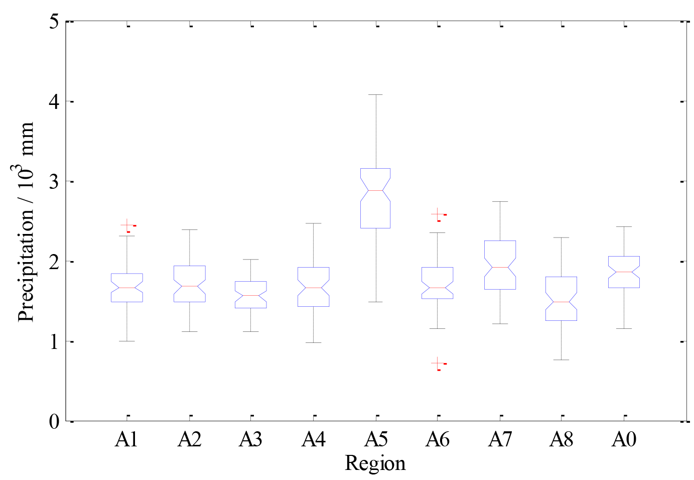
Figure 3Box plot of precipitation of sub-regions and the entire region. The upper and lower boundaries of the box were set to the values of their percentiles as one-quarter and three-quarters, Q1 and Q3, respectively. The red solid line refers to the median. The upper and lower boundaries extended along the dashed line were further set to the values as and , respectively. The values beyond extended boundaries were generally regarded as abnormal, marked by the red plus sign.
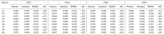
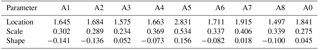
The statistics of the goodness-of-fit test of four alternative univariate distributions were smaller than those of the significance level of 0.05 (see Table 3), which implied that the GEV, GLO, P-III and GNO distributions fitted annual precipitation of the sub-regions and the entire region. The RMSE and AIC values among the distributions slightly differed and those of the GNO distribution were the smallest for most regions. Then, as illustrated in Fig. 4, all lines of the theoretical CDF almost overlapped the points of the empirical CDF. They demonstrated that the GNO satisfactorily fitted the frequency distributions of annual precipitation for the entire region and sub-regions. As shown in Table 4, the shape parameters of the GNO in the A1 and A2 sub-regions were clear minus, that in the A5 sub-region was clear positive and others were close to zero, which implied significantly left-skewed, right-skewed and normal distributions, respectively.
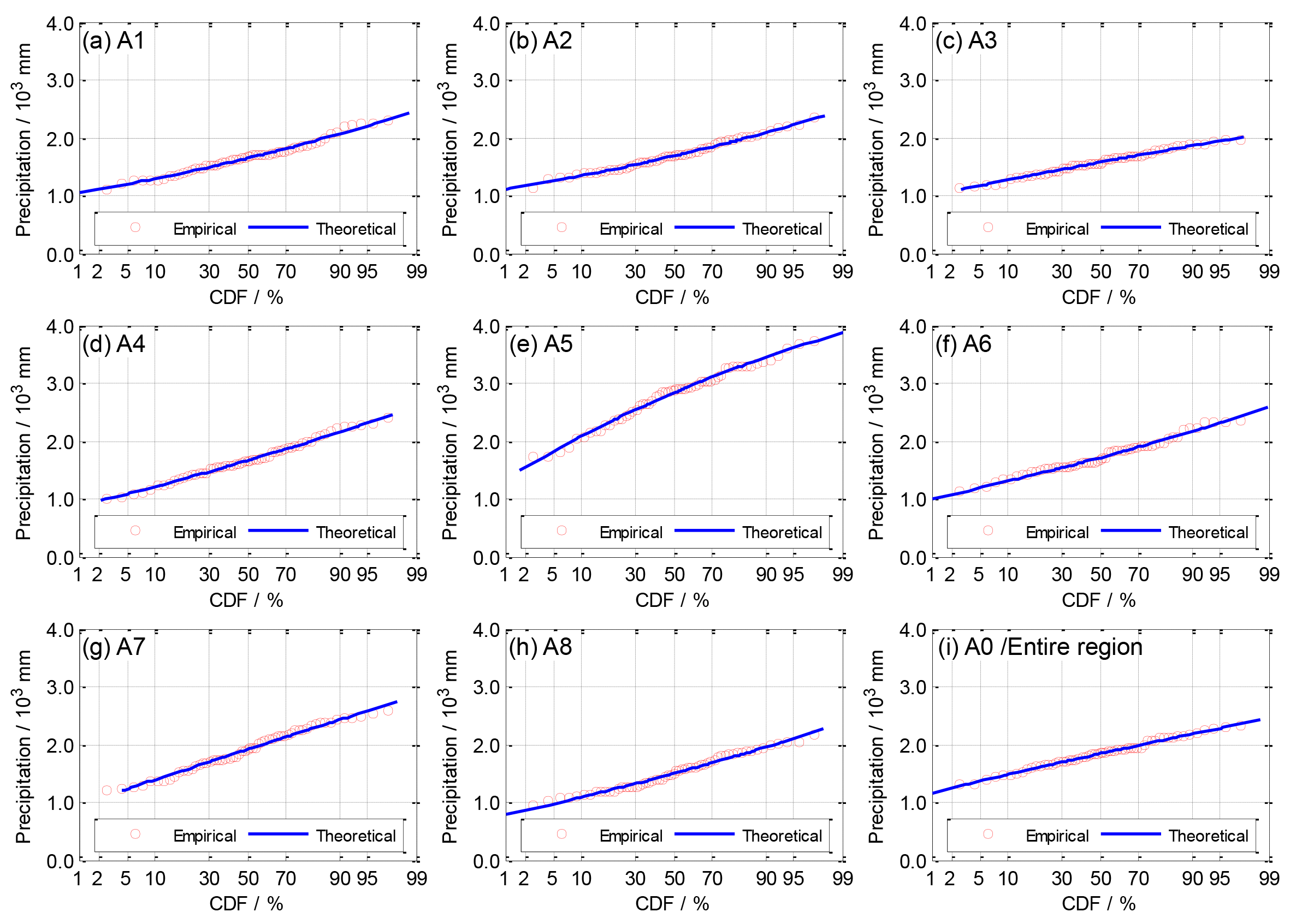
Figure 4Empirical and theoretical CDFs of precipitation of sub-regions and the entire region using the GNO distribution. On the x axis, the Hessian scale transferred by using the standard normal distribution was used.
Table 3Goodness-of-fit test of univariate distributions of precipitation of sub-regions and the entire region. The standard (value) refers to the statistic of the significance level of 0.05.
4.2 Eight-dimensional joint distribution of sub-regional precipitation
A matrix of correlation coefficients between sub-regional precipitations is illustrated in Fig. 5. Due to the geographical distance and direction, the coefficients varied from different pairs of sub-regions, but most of them were quite large except between A8 and other sub-regions, such as both A8–A6 and A8–A4, which were less than 0.1. In actuality, the correlation coefficient implied dependence between sub-regional precipitation values. The larger the coefficient was, the larger the dependence was.
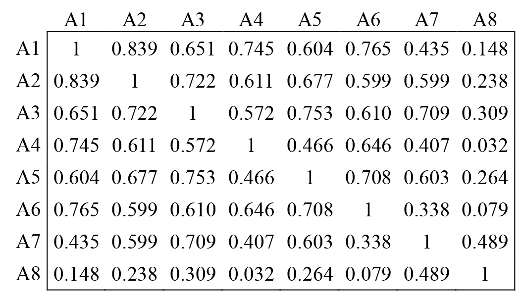
Table 4Parameters of the GNO distribution of precipitation of sub-regions and the entire region.
The Q-Q plot of empirical and theoretical joint CDFs showed that the sample points fell near the diagonal of 1:1, though more fell in the lower tail (see Fig. 6). For the goodness-of-fit test of the eight-dimensional meta-Gaussian copula, the p-value accounted for 0.262 beyond the significance level of 0.05. This demonstrated that the high-dimensional Gaussian copula better fitted the joint distribution of precipitation of eight sub-regions. However, eight-dimensional joint CDFs of sub-regional precipitation on the basis of observed data were limited and the maximum was less than 0.75.
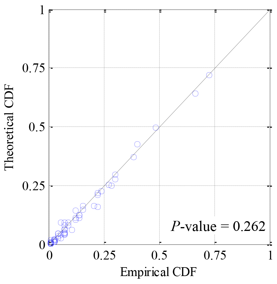
Figure 6Q–Q plot of empirical and theoretical CDFs of sub-regional precipitation using the eight-dimensional Gaussian copula.
When the conventional joint CDF of sub-regional precipitation was transformed into the Kendall CDF, the CDF was indeed enlarged (see Fig. 7a). For example, using observed data, the minimum of 0.00005 and the maximum of 0.71957 for the conventional joint CDF corresponded to 0.00916 and 0.99084 for the Kendall CDF, respectively. Using the Hessian axes in which the scales of dual axes were transferred following the standard normal distribution (see Fig. 7b), the conventional joint CDF and the Kendall CDF showed a linear relationship, which demonstrated that it was appropriate to use the Kendall instead of the conventional joint CDF.
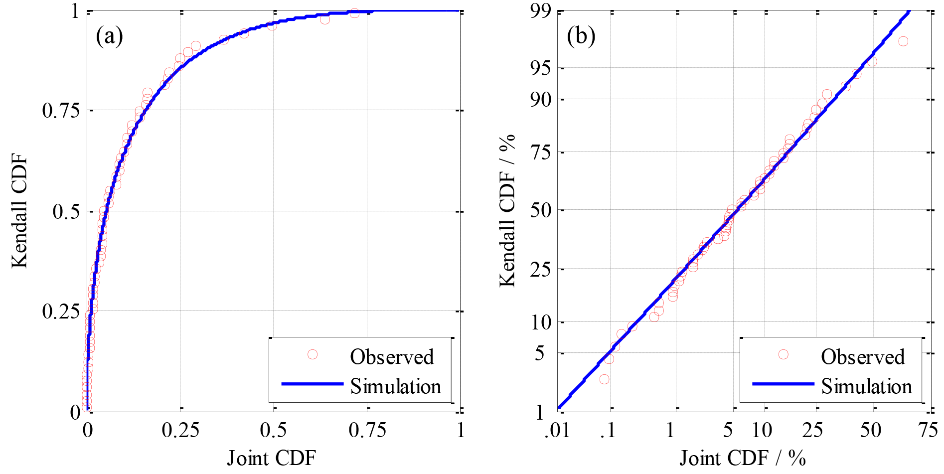
Figure 7Comparison of conventional joint CDF and Kendall CDF in subfigures (a) with the general axes and (b) with the Hessian axes.
4.3 Relationship between sub-regional joint and entire region CDFs of precipitation
According to the determined eight-dimensional Gaussian copula, a million combinations of CDFs of sub-regional precipitation were generated by using Monte Carlo simulation. Correspondingly, the conventional joint and Kendall CDFs of sub-regions and the CDFs of the entire region were achieved (illustrated in Fig. 8). Comparing the conventional joint and the entire region CDFs (see Fig. 8a), the combination points tended to happen in the northwest and had an up-convex lower boundary. When the CDF of the entire region was given a certain value, the corresponding joint CDFs varied within the limited upper bound on which the joint CDFs were less than the given value of the entire region.
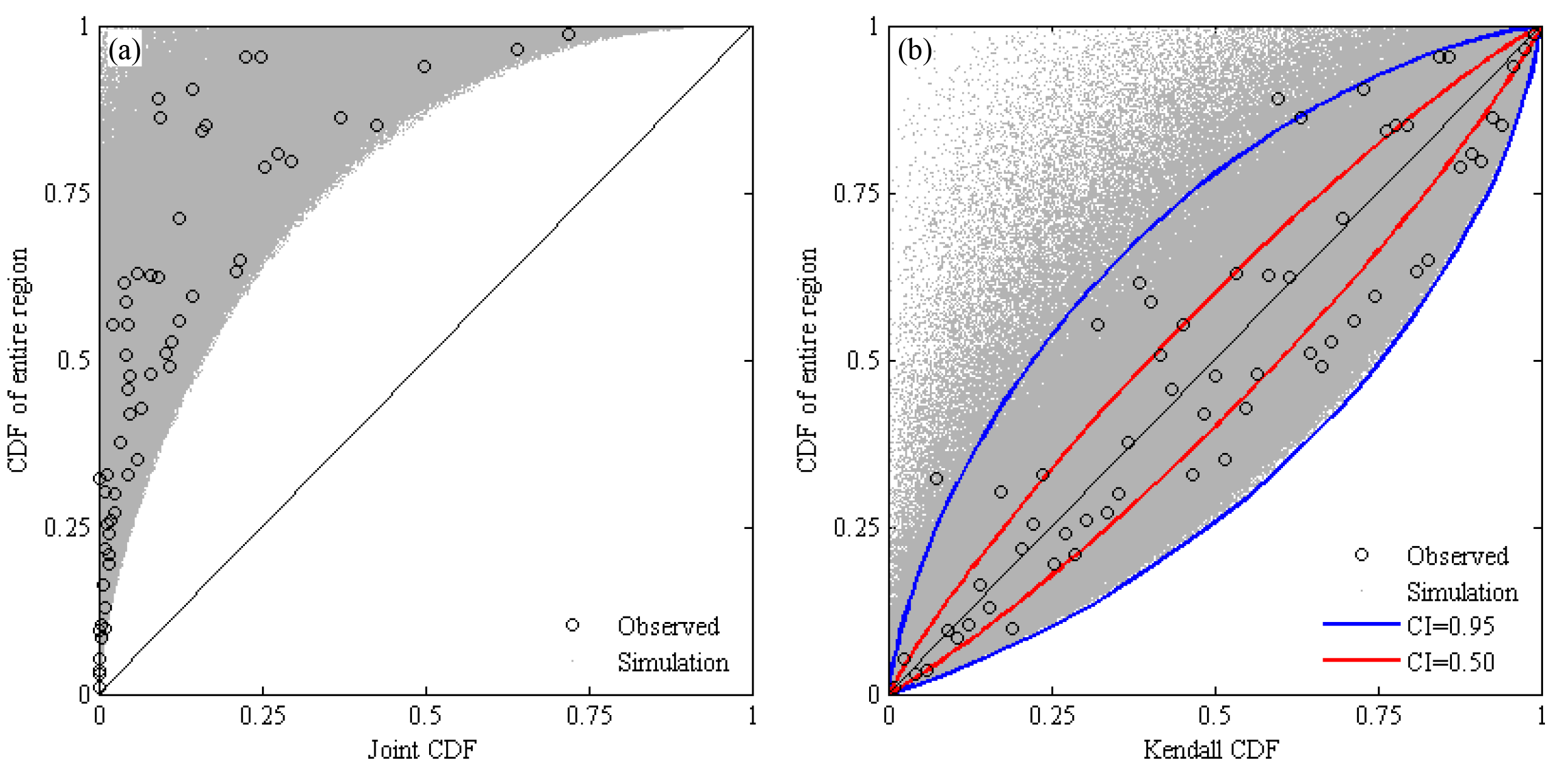
Figure 8CDF of precipitation of the entire region responding to (a) the conventional joint CDF and (b) the Kendall CDF of eight sub-regions.
Using the Kendall CDF instead of the conventional joint CDF (see Fig. 8b), the combination points scattered near the diagonal of 1:1 with a concave upper lower boundary. It also showed that most observed samples fell within the envelope of CI with a probability of 0.95. In addition, between the Kendall CDF and the CDF of the entire region, there were large correlation coefficients of 0.9221 and 0.9153 for the observed and simulated samples, respectively. These showed that the Kendall CDF instead of the conventional CDF was convenient to analyze the relationship of the CDF between the entire region and the sub-regional joint CDF.
4.4 Design combinations of the CDF of sub-regional precipitation
The given CDFs of precipitation of the entire region can be predefined to change in the range from 0.05 to 0.95 with a step of 0.05, which refers to the alteration of regional precipitation from extreme dry to extreme wet. Considering the uncertainty of Monte Carlo simulation, those simulated combinations (see grey points in Fig. 9), in which the allowable relative error of their calculated CDFs of the entire region compared to a given CDF was less than 0.05 %, were selected to be an alternate for further design combination.
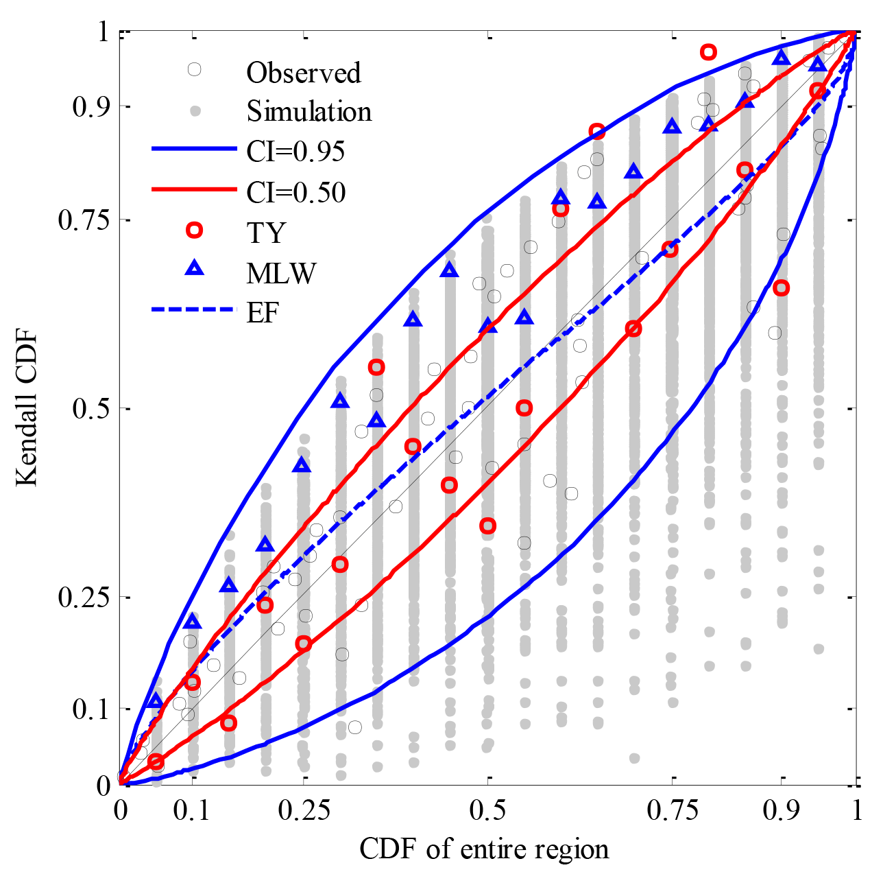
Figure 9Design Kendall CDFs for given CDFs of precipitation of the entire region which varied from 0.05 to 0.95 with a step of 0.05.
Using the EF method (see the blue dashed line in Fig. 9), design points consisted of a better smooth curve which mostly fell within 0.5 of the CI. The Kendall CDF was very close to the CDF of the entire region, but that of the former was larger than that of the latter, with lower CDFs being less than 0.55 in the study case, and vice versa in larger CDFs. Using the TY method (see the red circles in Fig. 9), design points were irregularly scattered on the two sides of the diagonal of 1:1, and even several points were beyond 0.95 of the CI, for example for the given CDFs of 0.8 and 0.9. Using the MLW method (see the blue triangles in Fig. 9), design points fell within the range between 0.5 and 0.95 of the CI, and design Kendall CDFs were larger than the given CDFs.
In general, if the CDF of sub-regional precipitation was equalized, the differences between the design Kendall CDF and the given CDF of the entire region were almost no more than a CI of 0.5. On the basis of maximum joint probability density, design Kendall CDFs were larger than the given CDFs and preferred to the upper limited bound. By zooming in or out according to the typical year, design points almost fell within 0.95 of the CI, but they were relatively scattered in comparison to other methods.
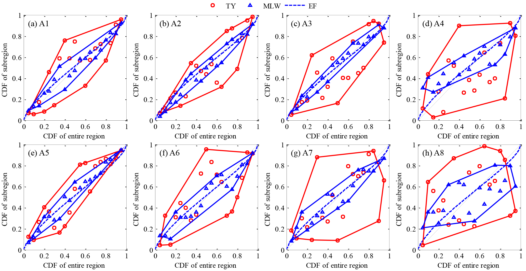
In addition, between individual CDFs of eight sub-regional precipitations and the CDF of the entire region, the design points maintained a smooth curve and were undifferentiated for all sub-regions when using the EF method (see the blue dashed line in Fig. 10). The design individual CDFs of sub-regions were very close to the CDF of the entire region, but the former were larger than the latter in the lower CDFs and vice versa in the larger CDFs. Using TY and MLW methods, design points were scattered on the two sides of the diagonal of 1:1. Design CDFs differed from sub-regions, but their differences were undetermined. However, as seen from the envelope of design points of individual sub-regions, the ranges of the MLW design were comparatively narrow and concentrated around the diagonal of 1:1 except for the A8 sub-region, but those of the TY design were much wider, in particular for the A4, A7 and A8 sub-regions.
4.5 Design water demand of irrigation
For given CDFs of precipitation of the entire region, the water demand of irrigation of the entire region for all selected simulations and design points are illustrated in Fig. 11a. As the given CDF changed from 0.05 to 0.95, the average value of water demand decreased from 22.79 to 12.78 billion m3, correspondingly representing the range from extremely dry to extremely wet (see the black dashed line in Fig. 11a). The difference between the maximum and minimum demands for a given CDF (see the blue and red dashed lines in Fig. 11a) varied in the range of 1.15–1.72 billion m3. Design demands of the MLW and EF methods (see the blue and black solid lines in Fig. 11a) were slightly smaller than the average values, but those of the TY method (see the red line in Fig. 11a) fluctuated around the line of average value. Compared to the average values (see Fig. 11b), the maximum and minimum demands increased and decreased by 3.0 %–7.5 % and 2.5 %–3.8 %, respectively. Design demands of the MLW and EF methods decreased within 1.4 % and 2.1 %, respectively, and those of the TY method increased or decreased within 2.8 % or 2.1 %, respectively. These values demonstrated that the differences of water demand among three design methods for the entire region were quite small.
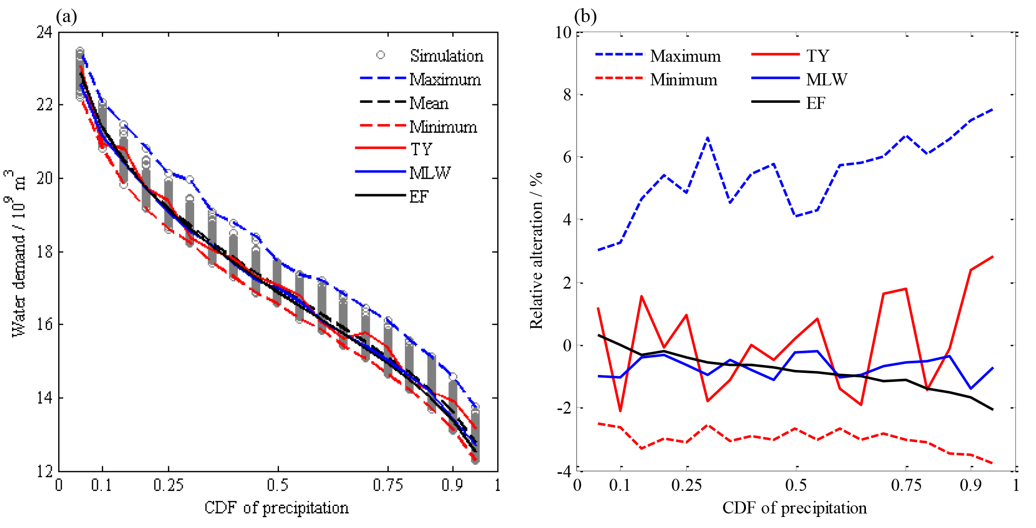
Figure 11(a) Design water demand of irrigation of the entire region and (b) their relative alteration compared to the average demand.
Design water demands of irrigation in individual sub-regions are illustrated in Fig. 13. As the given CDF changed from 0.05 to 0.95, sub-regional demands of the EF method smoothly decreased from 2.16–3.73 to 1.16–2.29 billion m3, correspondingly representing the range from extremely dry to extremely wet (see the black lines in Fig. 12). Then, the demands of the TY and MLW methods fluctuated around the lines of the demand of the EF method, and the fluctuations of the former were remarkably larger than those of the latter (see the red and blue lines in Fig. 12). Compared to the EF method (see Fig. 13), the increase or decrease in the water demand of the MLW design accounted for less than 13 % in most sub-regions, except for the A8 sub-region with a maximum of 26.1 %, but that of the TY method accounted for 15.4 %–24.3 % for the A1, A2, A3 and A5 sub-regions and 39.8 %–45.7 % for the A4, A6, A7 and A8 sub-regions. These values demonstrated that the alterations of design water demand in sub-regions were more complicated in comparison with those in the entire region.
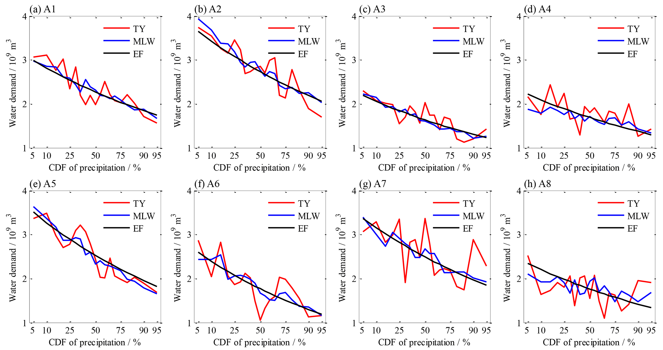
Figure 12Design water demand of irrigation in sub-regions for given CDFs of precipitation of the entire region.
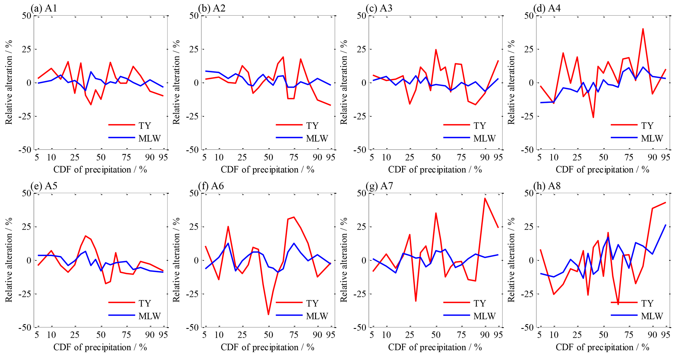
Figure 13Relative alteration of design water demand compared to the EF method for given CDFs of precipitation of the entire region.
Using Guangdong Province of South China as a case study of a large region, a high-dimensional meta-Gaussian copula was applied for fitting the joint distribution of multiple regional precipitation. A large number of combinations of CDFs of precipitation of eight sub-regions were generated by using the Monte Carlo method. The relationship among the CDFs of the entire region, the conventional joint CDF, and the Kendall CDF of sub-regions was determined. Three design methods, including the EF and TY design methods, and a new design procedure of the MLW method in association with the joint probability density, were used for design combinations of sub-regional CDFs for given CDFs of precipitation of the entire region. Then, design water demands of irrigation of the entire region and individual sub-regions were compared. The main conclusions of this study are as follows.
-
The frequency distributions of annual precipitation of the entire region and of sub-regions were fitted well by the GNO distribution. The shape parameters in the A1 and A2 sub-regions were a clear minus, those in the A5 sub-region were a clear positive, and others were close to zero, which implied significantly left-skewed, right-skewed and normal distributions, respectively. The eight-dimensional Gaussian copula satisfactorily fitted the joint distribution of sub-regional precipitation.
-
There was a clear linear dependence between the conventional joint and Kendall CDFs of sub-regional precipitation when both of them were transferred by the standard normal distribution. Comparing the Kendall CDFs of sub-regions and the CDF of the entire region, most observed samples fell within the envelope of CI of a probability of 0.95 around the diagonal of 1:1, and there were greater dependences between them with correlation coefficients of 0.9221 and 0.9153 for the observed and simulated samples, respectively. The use of the Kendall CDF instead of the conventional joint CDF can better link the joint frequency of sub-regions and the univariate frequency of the entire region. However, any one given CDF of the entire region corresponded to a large number of joint CDFs varying from very small to limited large CDFs. That is, there was an upper bound in larger values of the joint CDFs of sub-regions corresponding to given CDFs of the entire region.
-
For given CDFs of precipitation of the entire region, design Kendall CDFs and individual CDFs of eight sub-regions of the EF method maintained a smooth curve and were very close to their diagonal of 1:1. The design Kendall CDFs of the MLW method which were larger than the given CDFs of the entire region fell between 0.5 and 0.95 probabilities for the CI far from the diagonal, and those of the TY method were irregularly scattered on the two sides of the diagonal. Then, design CDFs of individual sub-regions of the MLW and TY methods were also scattered on the two sides of the diagonal, but they differed for individual sub-regions. The change ranges of the MLW design were comparatively narrow and were concentrated around the diagonal, but those of the TY design were much wider.
-
For given CDFs varying from 0.05 to 0.95 representing the range from extremely dry to extremely wet, the simulated water demand of irrigation of the entire region in terms of the average value accounted for from 22.79 to 12.78 billion m3. Design demands of the MLW and EF methods were slightly smaller than the average values, and those of the TY method fluctuated around the average values. Compared to the average demand, design demands of the MLW, EF and TY methods decreased or increased, respectively, within 1.4 %, 2.1 %, and 2.8 %, which demonstrated that the differences of design demand of the entire region among the three methods were quite small.
-
For given CDFs varying from 0.05 to 0.95 representing the range from extremely dry to extremely wet, design water demands of individual sub-regions of the EF method decreased smoothly from 2.16–3.73 to 1.16–2.29 billion m3, and those of the MLW and TY methods fluctuated around the demand lines of the EF method, but the fluctuations of the TY method were remarkably larger than those of the MLW method. Compared to the EF method, the increase or decrease in the water demand of the MLW design accounted for less than 13 % in most sub-regions, except for the A8 sub-region with a maximum of 26.1 %, but those of the TY method accounted for 39.8 %–45.7 % for the A4, A6, A7 and A8 sub-regions. These values demonstrated that the alterations of design water demand in sub-regions were more complicated in comparison with those in the entire region.
All in all, in practical planning of regional water resources, using the EF method can realize water demand of irrigation for the entire region and its sub-regions for a given frequency of precipitation, but it is arbitrary that the series of sub-regional precipitation are regarded to be undifferentiated for a large region, for example the case region. The TY method was constrained by the limited observed data of precipitation and it cannot be chosen when several different combinations of sub-regional precipitation made the frequency of precipitation of the entire region approximately identical. Therefore, a design procedure using the MLW method in association with a high-dimensional copula, which simulated individual univariate distributions, captured their dependences for multi-variables and built a linkage between regional frequency and sub-regional frequency of precipitation, is recommended for design water demand of irrigation for a large region.
Precipitation data used in this study were obtained from the Surface Climate Daily Data Set of China and are available upon request. Address inquiries to the corresponding author.
XJT conceived this study and developed the method and wrote the paper. YLD conducted modelling experiments and performed the analysis. VPS revised the manuscript. XHC and KRL contributed comments on the method and writing. HOW conducted data analysis.
The authors declare that they have no conflict of interest.
Support by the National Key R&D Program of China (2017YFC0405900), the
National Natural Science Foundation of China (51479217; 51879288), and the
Outstanding Youth Science Foundation of NSFC (51822908) is gratefully
acknowledged.
Edited by: Luis
Samaniego
Reviewed by: two anonymous referees
Abdul Rauf, U. F. and Zeephongsekul, P.: Copula based analysis of rainfall severity and duration: a case study, Theor. Appl. Climatol., 115, 153–166, 2014.
Aussenegg, W. and Cech, C.: A new copula approach for high-dimensional real world portfolios, Working Paper Series by the University of Applied Sciences bfi Vienna, 68, 1–33, https://www.researchgate.net/publication/267391266, 2012.
Barbe, P., Genest, C., Ghoudi, K., and Remillard, B.: On Kendall's process, J. Multivar. Anal., 58, 197–229, 1996.
Cai, J. B., Liu, Y., Cai, L. Z., and Wu, Y. Y.: A method of determining suitable probability for irrigation project design, Irrig. Drain., 20, 30–31, 2001 (in Chinese).
Cai, X., Hejazi, M. I., and Wang, D.: Value of probabilistic weather forecasts: assessment by real–time optimization of irrigation scheduling, J. Water Resour. Plann. Manage., 137, 391–403, 2011.
Chen, L., Singh, V. P., Guo, S., and Zhou, J.: Copula-based method for multisite monthly and daily streamflow simulation, J. Hydrol., 528, 369–384, 2015.
Chowdhary, H., Escobar, L. A., and Singh, V. P.: Identification of suitable copulas for bivariate frequency analysis of flood peak and flood volume data, Hydrol. Res., 42, 193–215, 2011.
Corbella, S. and Stretch, D. D.: Multivariate return periods of sea storms for coastal erosion risk assessment, Nat. Hazards Earth Syst. Sci., 12, 2699–2708, https://doi.org/10.5194/nhess-12-2699-2012, 2012.
Creal, D. D. and Tsay, R. S.: High dimensional dynamic stochastic copula models, J. Econometrics, 189, 335–345, 2015.
Davidson, B. and Hellegers, P.: Estimating the own–price elasticity of demand for irrigation water in the Musi catchment of India, J. Hydrol., 408, 226–234, 2011.
Dobric, J. and Schmid, F.: A goodness of fit test for copulas based on Rosenblatt's transformation, Comput. Stat. Data Anal., 51, 4633–4642, 2007.
Ganguli, P. and Reddy, M. J.: Evaluation of trends and multivariate frequency analysis of droughts in three meteorological subdivisions of western India, Int. J. Climatol., 34, 911–928, 2014.
Genest, C. and Rivest, L. P.: Statistical inference procedures for bivariate Archimedean copulas, J. Am. Stat. Assoc., 88, 1034–1043, 1993.
Genest, C., Favre, A. C., Béliveau, J., and Jacques, C.: Metaelliptical copulas and their use in frequency analysis of multivariate hydrological data, Water Resour. Res., 43, 223–236, 2007.
Genest, C., Remillard, B., and Beaudoin, D.: Goodness–of–fit tests for copulas: a review and a power study, Insur. Math. Econ., 44, 199–213, 2009.
Gohari, A., Eslamian, S., Abedi-Koupaei, J., Bavani, A. M., Wang, D. B., and Madani, K.: Climate change impacts on crop production in Iran's Zayandeh-Rud River Basin, Sci. Total Environ., 442, 405–419, 2013.
Gräler, B., van den Berg, M. J., Vandenberghe, S., Petroselli, A., Grimaldi, S., De Baets, B., and Verhoest, N. E. C.: Multivariate return periods in hydrology: a critical and practical review focusing on synthetic design hydrograph estimation, Hydrol. Earth Syst. Sci., 17, 1281–1296, https://doi.org/10.5194/hess-17-1281-2013, 2013.
Griffin, R. C.: Achieving water use efficiency in irrigation districts, J. Water Resour. Plann. Manage., 132, 434–442, 2006.
Gringorten, I. I.: A plotting rule for extreme probability paper, J. Geophys. Res., 68, 813–814, 1963.
Lankford, B.: Localising irrigation efficiency, Irrig. Drain., 55, 345–362, 2010.
Leenhardt, D., Trouvat, J. L., Gonzalès, G., Peramaud, V., Prats, S., and Bergez, J. E.: Estimating irrigation demand for water management on a regional scale: II. Validation of ADEAUMIS, Agr. Water Manage., 68, 207–232, 2004.
Leenhardt, D., Angevin, F., Biarnès, A., Colbach, N., and Mignolet, C.: Describing and Locating Cropping Systems on a Regional Scale, in: Sustainable Agriculture, Vol. 2, Springer, Netherlands, 85–95, 2011.
Lian, J., Xu, K., and Ma, C.: Joint impact of rainfall and tidal level on flood risk in a coastal city with a complex river network: a case study of Fuzhou City, China, Hydrol. Earth Syst. Sci., 17, 679-689, doi: 10.5194/hess-17-679-2013, 2013. Liu, Z., Guo, S., Li, T., Hu, Y., and Li, L.: Interval estimation method for design flood region composition, J. Hydraul. Eng., 46, 543-550, doi: 10.13243/j.cnki.slxb.20140928, 2015. (in Chinese)
Liu, Z., Guo, S., Li, T., Hu, Y., and Li, L.: Interval estimation method for design flood region composition, J. Hydraul. Eng., 46, 543–550, 2015 (in Chinese).
Massey, F. J.: The Kolmogorov–Smirnov test for goodness of fit, J. Am. Stat. Assoc., 46, 68–78, 2012.
Meza, F. J., Wilks, D. S., Gurovich, L., and Bambach, N.: Impacts of climate change on irrigated agriculture in the Maipo Basin, Chile: reliability of water rights and changes in the demand for irrigation, J. Water Resour. Plann. Manage., 138, 421–430, 2012.
Michele, C., Salvadori, G., Vezzoli, R., and Pecora, S.: Multivariate assessment of droughts: frequency analysis and dynamic return period, Water Resour. Res., 49, 6985–6994, 2013.
Nappo, G. and Spizzichino, F.: Kendall distributions and level sets in bivariate exchangeable survival models, Inform. Sci., 179, 2878–2890, 2009.
Nelsen, R. B.: An Introduction to Copulas, Springer, New York, 2006.
Rosenblatt, M.: Remarks on a multivariate transformation, Ann. Math. Stat., 23, 470–472, 1952.
Salvadori, G. and Michele, C. D.: Frequency analysis via copulas: Theoretical aspects and applications to hydrological events, Water Resour. Res., 40, 229–244, 2004.
Salvadori, G., De Michele, C., and Durante, F.: On the return period and design in a multivariate framework, Hydrol. Earth Syst. Sci., 15, 3293–3305, https://doi.org/10.5194/hess-15-3293-2011, 2011.
Salvadori, G., Durante, F., and Michele, C. D.: Multivariate return period calculation via survival functions, Water Resour. Res., 49, 2308–2311, 2013.
Serinaldi, F.: An uncertain journey around the tails of multivariate hydrological distributions, Water Resour. Res., 49, 6527–6547, 2013.
Tarjuelo, J. M., Olalla, F. D. S., and Pereira, L. S.: Land and water use: environmental management tools and practices – Preface, Agr. Water Manage., 77, 1–3, 2005.
Thomas, A.: Agricultural irrigation demand under present and future climate scenarios in China, Global Planet. Change, 60, 306–326, 2008.
Tu, X., Singh, V. P., Chen, X., Ma, M., Zhang, Q., and Zhao, Y.: Uncertainty and variability in bivariate modeling of hydrological droughts, Stoch. Environ. Res. Risk A., 30, 1317–1334, 2016.
Tu, X., Du, Y., Chen, X., Chai, Y., and Qing, Y.: Modeling and design on joint distribution of precipitation and tide in the coastal city, Adv. Water Sci., 28, 49–58, 2017a (in Chinese).
Tu, X., Du, X., Singh, V. P., Chen, X., Du, Y., and Li, K.: Joint Risk of Interbasin Water Transfer and Impact of the Window size of Sampling low flows under Environmental Change, J. Hydrol., 554, 1–11, 2017b.
Volpi, E. and Fiori, A.: Hydraulic structures subject to bivariate hydrological loads: Return period, design, and risk assessment, Water Resour. Res., 50, 885–897, 2014.
Wisser, D., Frolking, S., Douglas, E. M., Fekete, B. M., Vorosmarty, C. J., and Schumann, A. H.: Global irrigation water demand: Variability and uncertainties arising from agricultural and climate data sets, Geophys. Res. Lett., 35, L24408, https://doi.org/10.1029/2008GL035296, 2008.
Wriedt, G., Velde, M. V. D., Aloe, A., and Bouraoui, F.: Estimating irrigation water requirements in Europe, J. Hydrol., 373, 527–544, 2009.
Xie, H., Luo, Q., and Huang, J.: Synchronous asynchronous encounter analysis of multiple hydrologic regions based on 3D copula function, Adv. Water Sci., 23, 186–193, 2012 (in Chinese).
Yan, B., Guo, S., Chen, L., and Liu, P.: Flood encountering risk analysis for the Yangtze River and Qingjiang River, J. Hydraul. Eng., 41, 553–559, 2010a (in Chinese).
Yan, B., Guo, S., Guo, J., Chen, L., Liu, P., and Chen, H.: Regional design flood composition based on copula function, J. Hydraul. Eng., 29, 60–65, 2010b (in Chinese).
Zhang, L. and Singh, V. P.: Bivariate flood frequency analysis using the copula method, J. Hydrol. Eng., 11, 150–164, 2006.
Zhang, Q., Li, J., Chen, X., and Bai, Y.: Spatial Variability of Probability Distribution of Extreme Precipitation in Xinjiang, Acta Geogr. Sin., 66, 3–12, 2011 (in Chinese).
Zhang, Q., Li, J., Singh, V. P., and Xu, C.: Copula-based spatio-temporal patterns of precipitation extremes in China, Int. J. Climatol., 33, 1140–1152, 2013.
Zhang, Q., Gu, X., Singh, V. P., Kong, D., and Chen, X.: Spatiotemporal behavior of floods and droughts and their impacts on agriculture in China, Global Planet. Change, 131, 63–72, 2015a.
Zhang, Q., Sun, P., Li, J., Singh, V. P., and Liu, J.: Spatiotemporal properties of droughts and related impacts on agriculture in Xinjiang, China, Int. J. Climatol., 35, 1254–1266, 2015b.
Zhang, Q., Xiao, M. Z., and Singh, V. P.: Uncertainty evaluation of copula analysis of hydrological droughts in the East River basin, China, Global Planet. Change, 129, 1–9, 2015c.