the Creative Commons Attribution 4.0 License.
the Creative Commons Attribution 4.0 License.
 | 06 Sep 2018
A geostatistical data-assimilation technique for enhancing macro-scale rainfall–runoff simulations
Alessio Pugliese
Simone Persiano
Stefano Bagli
Paolo Mazzoli
Juraj Parajka
Berit Arheimer
René Capell
Alberto Montanari
Günter Blöschl
Attilio Castellarin
Our study develops and tests a geostatistical technique for locally enhancing macro-scale rainfall–runoff simulations on the basis of observed streamflow data that were not used in calibration. We consider Tyrol (Austria and Italy) and two different types of daily streamflow data: macro-scale rainfall–runoff simulations at 11 prediction nodes and observations at 46 gauged catchments. The technique consists of three main steps: (1) period-of-record flow–duration curves (FDCs) are geostatistically predicted at target ungauged basins, for which macro-scale model runs are available; (2) residuals between geostatistically predicted FDCs and FDCs constructed from simulated streamflow series are computed; (3) the relationship between duration and residuals is used for enhancing simulated time series at target basins. We apply the technique in cross-validation to 11 gauged catchments, for which simulated and observed streamflow series are available over the period 1980–2010. Our results show that (1) the procedure can significantly enhance macro-scale simulations (regional LNSE increases from nearly zero to ≈0.7) and (2) improvements are significant for low gauging network densities (i.e. 1 gauge per 2000 km2).
- Article
(5454 KB) - Full-text XML
- BibTeX
- EndNote


The steady increase in computational capabilities together with the expanding accessibility of regional and global datasets (e.g. soil properties, land-cover, morphology, climate characteristics, satellite-based gridded precipitation) trigger the development of regional- to continental-scale and global-scale hydrological models (Archfield et al., 2015), hereafter referred to as macro-scale models.
During the last decade, several of these macro-scale models have become operational and thus continuously provide data automatically for decision-making. For instance, the distributed rainfall–runoff-routing model LISFLOOD (De Roo et al., 2000) provides daily forecast for operational warning services through the systems of EFAS (Pappenberger et al., 2013) and GLOFAS (Alfieri et al., 2013); the LARSIM models (Haag and Luce, 2008) are used operationally for simulating streamflow at large areas in southern Germany, Luxembourg, Austria, Switzerland, and the eastern part of France; the WATFLOOD, developed at the University of Waterloo, is used operationally in Canada (Kouwen et al., 1993); and the S-HYPE model (Strömqvist et al., 2012) is running operationally for flood or drought forecasting and water quality assessments for the Swedish landmass, providing high-resolution information to authorities and citizens (Hjerdt et al., 2011).
Other macro-scale models are used for off-line water assessments and research purposes. For instance, the global WaterGAP Global Hydrological model (Alcamo et al., 2003) assists in water accounting; the SAFRAN-ISBA-MODCOU model (Habets et al., 2008) has been applied over the entire French territory to combine a meteorological analysis system, a land surface model, and a hydrogeological model; the PGB-IPH model (Pontes et al., 2017) has been applied to many South American basins; and the SWIM model (Krysanova et al., 1998) couples water balance simulations with water quality for small to mid-size watersheds, i.e. regional meso-scale.
The macro-scale hydrological models are getting more and more popular due to three main reasons: (1) they can provide users with a large-scale representation of hydrological behaviour, which is fundamental information for effectively addressing several water resources planning and management problems (e.g. surface water availability assessment, instream water quality studies, ecohydrological studies); (2) they can be used to compute a variety of hydrological signatures everywhere along the stream network at the resolution of the model; (3) model outputs in some cases are open-access and freely distributed, so that their regional runs represent a wealth of information for addressing the problem of hydrological predictions in data-scarce regions of the world (Beck et al., 2016; Donnelly et al., 2016; Pechlivanidis and Arheimer, 2015). Accurate regional hydrological simulations undoubtedly foster and support the implementation of improved large-scale and trans-boundary policies for water resources system management and flood-risk mitigation or climate change adaptation (Arheimer et al., 2017; Falter et al., 2016; Sampson et al., 2015; de Paiva et al., 2013).
However, improved accuracy in terms of average regional performance does not necessarily imply homogeneous improvements in local performance. In fact, due to the difficulties to perform local calibrations and validations of macro-scale models over the entire modelled regions, local performance can be rather diverse (Donnelly et al., 2016; de Paiva et al., 2013). Factors controlling the heterogeneity of local performance may be various, for instance the quality of macro-scale input data, local water management, representativeness of model structure chosen, the influence of local geophysical and micro-climatic factors.
There is a recognized and noteworthy value in readily available and easy accessible simulated daily streamflow series for scarcely gauged, or ungauged, areas of the world to enhance awareness and decision-making (Arheimer et al., 2011; Hjerdt et al., 2011). Nevertheless, the harmonization and enhancement of local performances of macro-scale models is still a scientific challenge that is worth addressing in operational hydrology, and which raises different research questions, such as the following:
-
How could we deal with locally biased simulations?
-
Can we assimilate additional data to improve model performance without re-calibration?
-
Is there a minimum gauging network density that makes the post-modelling data assimilation viable and effective?
Recent literature shows the significant potential of kriging-based techniques for performing regional prediction of streamflow indices in ungauged locations (Castiglioni et al., 2011; Pugliese et al., 2014; Skøien et al., 2006). Among such techniques, topological kriging, or top-kriging (Skøien et al., 2006), has shown high prediction accuracy and excellent adaptability to a variety of water-related applications, such as prediction of low-flow indices (Castiglioni et al., 2009), interpolation of river temperatures (Laaha et al., 2013), estimation of flood quantiles (Archfield et al., 2013), regionalization of flow–duration curves (Castellarin, 2014; Castellarin et al., 2018; Pugliese et al., 2014, 2016), estimation of daily runoff in ungauged basins (Parajka et al., 2015) and reconstruction of historical daily streamflow series (Farmer, 2016).
Our study aims to develop and test a geostatistical data-assimilation procedure for better agreement between locally observed streamflow and model results from macro-scale rainfall–runoff models. The procedure employs top-kriging for geostatistically interpolating empirical period-of-record flow–duration curves (FDCs) along the stream network available at gauged basins. Interpolated FDCs are assimilated into simulated daily streamflow series at ungauged stream-network nodes, enhancing the local accuracy of simulated daily streamflow series. We test our method by improving E-HYPE model simulations (Donnelly et al., 2016; Hundecha et al., 2016), which provides approximately 30 years of simulated daily streamflows freely and openly accessible for 35 408 prediction nodes in Europe (mean catchment size of 215 km2, see also http://hypeweb.smhi.se/europehype/time-series/, last access: 30 July 2018). We address the Tyrolean region, as this area gives particularly poor simulations in the E-HYPE version 3 and thus would benefit from statistical enhancement of results. For the geostatistical interpolation, we use a group of 46 gauged catchments obtained from Austrian and Italian water services, and not used when setting up E-HYPE. With the observed streamflows we construct and interpolate empirical FDCs. Then, we assess the value and potential of assimilating this streamflow information into E-HYPE simulated series. In particular, (1) we cross-validate the proposed data-assimilation procedure for 11 E-HYPE prediction nodes located nearby an existing stream gauge, and (2) we assess the enhancement of simulated series resulting from the geostatistical data assimilation under different hypotheses on the spatial density of the stream-gauging network.
The paper is structured as follows: first, methods and procedures are presented in a general way, then we illustrate the case study and application. In particular, Sect. 2 presents the proposed procedure, while Sect. 3 details the system of cross-validations and sensitivity analyses we adopted for assessing the procedure. Section 4 illustrates the study area and E-HYPE simulation data. The last three sections report results, discussion and conclusions, respectively.
2.1 Geostatistical interpolation of empirical flow–duration curves (TNDTK)
Top-kriging is a powerful geostatistical procedure developed by Skøien et al. (2006) for the prediction of hydrological variables. Like all kriging approaches, top-kriging produces predictions of hydrological variables at ungauged sites with a linear combination of the empirical information collected at neighbouring gauging stations. Through this method, the unknown value of the streamflow index of interest at prediction location x0, Z(x0) can be estimated as a weighted average of the regionalized variable, measured within the neighbourhood:
where λj is the kriging weight for the empirical value Z(xj) at location xj, and n is the number of neighbouring stations used for interpolation. Kriging weights λj can be found by solving the typical ordinary kriging linear system (Eq. 2a) with the constraint of unbiased estimation (Eq. 2b):
where θ is the Lagrange parameter and γi,j is the semi-variance between catchment i and j (Isaaks and Srivastava, 1990). The semi-variance, or variogram, represents the spatial variability of the regionalized variable Z. Unique from any other method of kriging, top-kriging considers the variable defined over a non-zero support S, the catchment drainage area (Cressie, 1993; Skøien et al., 2006). The kriging system of Eqs. (2a) and (2b) remains the same, but the semi-variances between the measurements need to be obtained by regularization, i.e. smoothing the point variogram over the support area.
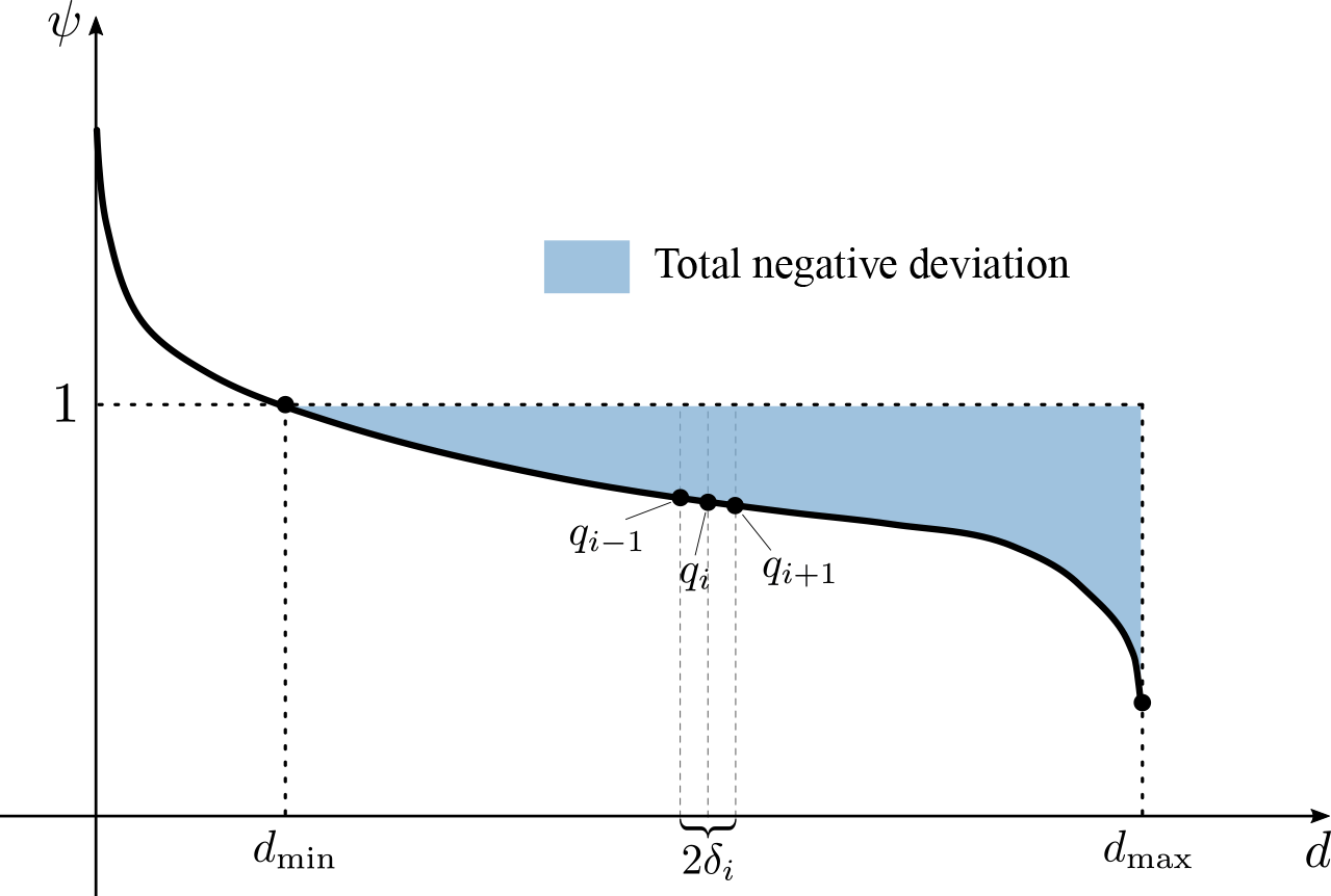
The point variogram can then be back-calculated by fitting aggregated variogram values to the sample variogram (Skøien et al., 2006). Pugliese et al. (2014) proposed a method for using top-kriging to predict FDCs at ungauged locations that they termed total negative deviation top-kriging (TNDTK). The authors reduce the dimensionality of the problem by seeking a unique index of site-specific FDCs. Unlike other regional approaches (Castellarin et al., 2013), the kriging-based method interpolates the entire curve, therefore ensuring its monotonicity (Castellarin, 2014; Pugliese et al., 2014). This is accomplished by first standardizing the empirical FDCs at site x, Ψ(x, d), for some reference value, Q*(x), to yield a dimensionless FDC:
where d denotes a specific duration. Pugliese et al. (2014) identified an overall point index that effectively summarizes the entire curve. This index, which the authors termed total negative deviation (TND), is derived by integrating the area between the lower limb of the FDC and the reference streamflow value Q* (see Fig. 1). Empirical TND values are computed as follows:
where represents the ith empirical dimensionless quantile standardized for the selected reference value Q*, δi is half of the frequency interval between the (i+1)th and (i−1)th quantile and the summation involves only the m standardized quantiles lower than 1. The equality between a given streamflow value and the reference value Q* is represented by a horizontal dashed line in Fig. 1, i.e. the threshold given by the equation . The range of the summation, m, in Eq. (4) is a function of the maximum duration dmax, which is itself a function of that sample with minimum length across gauged sites in the study region. Having calculated empirical TNDs, Pugliese et al. (2014) propose using the TNDs as a regionalized variable to develop site-specific weighting schemes. The same weights, derived through the solution of the linear kriging system (Eqs. 2a and 2b), are used for a batch prediction of the continuous, dimensionless FDC for the ungauged site x0:
where λj, with j=1, …, n, is the weights resulting from the kriging interpolation of TNDs, ψ(xj, d) is the dimensionless empirical FDC at the donor site xj, and , d) is the predicted dimensionless FDC. It is worth highlighting that the computation of the linear kriging system (Eqs. 2a and 2b) depends on n, the number of neighbouring sites on which to base the spatial interpolation, a fact that will be explored below.
If a reliable model for predicting Q* at the ungauged site x0 can be developed, the prediction of the dimensional FDC, , d), is obtained as follows:
where is the prediction of Q* at the ungauged site x0 and , d) has the same meaning as in Eq. (5).
The main objective of our study is to improve rainfall–runoff model simulations, whereas an assessment of the reliability of the regional metric TND is out of the scope of this paper. Nevertheless, further details on TNDTK (i.e. cross-validations in different geomorphological and climatic regions, sensitivity analyses, comprehensive assessments and comparisons to state-of-the-art models for predicting FDCs in ungauged basins) are reported in recent studies to which an interested reader is referred (Kim et al., 2017; Pugliese et al., 2014, 2016).
2.2 Algorithm for assimilation of local streamflow data
Following the approach proposed by Smakhtin and Masse (2000), we present a novel procedure for predicting the model residuals that may be associated with macro-scale rainfall–runoff model simulations (e.g. LISFLOOD, HYPE, PGB-IPH; see Introduction). This method relies on a regional prediction of the long-term FDC in the same site where these simulations are available.
For instance, let Ψ(x0, d) be the “true” unknown FDC for a given catchment x0 and , d) be its prediction constructed on the basis of the daily streamflows simulated through the macro-scale model. We can assume that a general relationship between the two curves exists and reads as follows:
where ε(x0, d) are the model residuals defined over the duration domain d, which we may term the residual–duration curve (εDC). Evidently, although the “true” residual–duration curve is unknown at ungauged basins, one can nevertheless estimate such a curve on the basis of geostatistically interpolated flow–duration curves , d) introduced in Sect. 2.1,
The estimated residual–duration curve obtained from the regional prediction of the long-term flow–duration curve can then be used for assimilating local streamflow information into the simulated daily streamflow series. The procedure is sketched in Fig. 2: (1) given a simulated streamflow series (red line in the top-right), select a specific day t and the corresponding discharge Q(t); (2) retrieve the duration d associated with Q(t) from the flow–duration curve constructed from simulated data (red line in the top-left quadrant); (3) read the estimated residual off of the predicted residual–duration curve (blue line in the bottom-left quadrant); and (4) assimilate the residual into the simulated series as . The iteration of the algorithm through all time steps leads to an enhanced simulated series (blue line in the top-right quadrant).
This new assimilation procedure shares some analogies with a technique called “quantile mapping”, used in the context of bias corrections for global climate model predictions (Komma et al., 2007). The procedure we propose in this context, though, is a rather general tool that can be applied to, for example, any macro-scale rainfall–runoff model for locally enhancing long simulated streamflow series without the need to re-run computationally intensive simulations, provided that the model itself is behavioural and validated on the basis of streamflow data that were not available for model calibration. The performance of the assimilation procedure depends on a variety of drivers, e.g. the quality of the simulated streamflows, which can be severely impacted by the local quality of input data even for a behavioural and well-calibrated model, the quality of streamflow data and the density of the stream-gauging network (see Sect. 3.1.3), the accuracy of the chosen regional model for predicting FDCs (Castellarin, 2014; Castellarin et al., 2013). Regarding the latter element, indeed, the proposed procedure deeply relies on accurate regional FDC predictions by means of an unbiased regional model, which necessarily must be validated beforehand for the area of interest. Otherwise, detriments are likely to be expected.
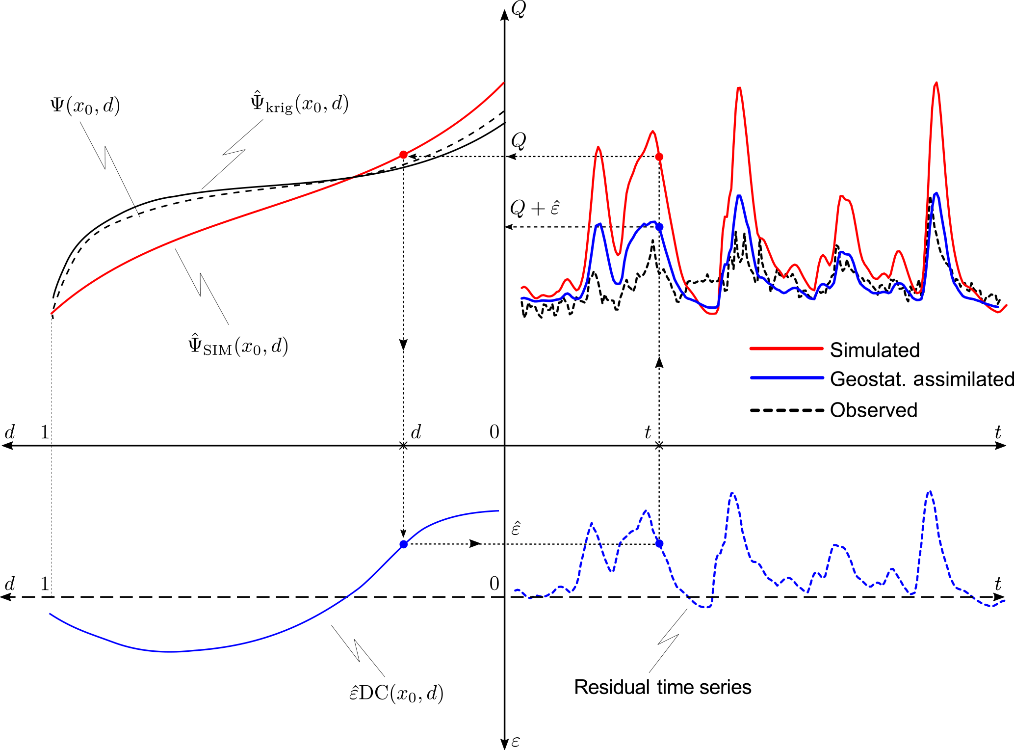
Figure 2Illustration of the proposed data-assimilation procedure for a given simulated time series. Top-right panel: real streamflow series (unknown, since the basin is ungauged, black dashed line); macro-scale model simulation (red solid line); geostatistically enhanced streamflow series (blue solid line). Top-left panel: FDC predictions obtained from simulated streamflows (red solid line) and via geostatistical interpolation (black solid line), with real (unknown) FDC (black dashed line). Bottom-left panel: estimated residual–duration curve (blue solid line) computed as the difference between the two predicted FDCs in the top-left panel. Bottom-right panel: time series of residuals (blue dashed line).
3.1 Structure of the analysis
The rationale of the analyses implemented in this study drives a sequence of operations, which can be summarized as follows:
-
Streamflow simulations from a given model, e.g. a rainfall–runoff macro-scale model, are available in a well-defined study area.
-
We suppose that recorded streamflow data are made available for a reasonable number of stream gauge stations within the study area, and we apply a suitable model for the regionalization of FDCs.
-
We validate the regional model with respect to available streamflow observations. In this case we adopted a leave-one-out cross-validation (Kroll and Song, 2013; Salinas et al., 2013; Srinivas et al., 2008; Wan Jaafar et al., 2011), even though different validation schemes might be preferred in other regions (Castellarin et al., 2018; Pugliese et al., 2016).
-
We validate the assimilation procedure by sequentially (a) neglecting all the streamflow information at a given nodes of the river network, (b) predicting FDCs, and (c) applying the assimilation method illustrated in Sect. 2.2.
-
We evaluate the sensitivity of the assimilation procedure to the stream gauge density of the study area.
The methodologies adopted for addressing points 3–5 are illustrated in Sects. 3.1.1, 3.1.2, and 3.1.3, in this order; the accuracy of predictions (e.g. regional FDCs, assimilated and simulated streamflow series) relative to their empirical or observed counterparts is quantified through performance indices described in Sect. 3.2.
3.1.1 Cross-validation of the FDC geostatistical interpolator (point 3 above)
We proposed to assess the accuracy of the geostatistical predictor of FDCs (i.e. TNDTK, see Sect. 2.1) in cross-validation with respect to available streamflow observations from a sufficient number of gauged catchments. We chose the mean annual flow (MAF), computed as the average flow of recorded historical streamflow series, as the reference value Q* (see details in Sect. 2.1).
TNDTK operates by first applying top-kriging to empirical TND values (see Sect. 2.1), which we performed by calculating a binned sample variogram first, and then by modelling binned empirical data with a five-parameter “modified” exponential theoretical variogram (Skøien et al., 2006). The fitted theoretical point variogram and its five parameters were obtained through the weighted least squares (WLS) regression method from Cressie (1993) by simultaneously fitting all regularized binned variograms that were computed for various area classes (Skøien, 2018). Recent applications of TNDTK indicate n=6 as an optimal number of neighbouring donor stations, and thus we chose the same value for this case study as well (Pugliese et al., 2014, 2016). Then, TNDTK uses the kriging weights obtained for predicting TND values for interpolating the dimensionless FDCs at the location of interest as the weighted average of dimensionless empirical FDCs constructed from the n=6 neighbouring gauged sites (see Eq. 5, in which λj, with j=1, …, 6 and n=6, is the kriging weights). While the computation of TNDs does not require any specific resampling scheme of the FDCs, the prediction of the curves in ungauged locations is carried out using a fixed number of quantiles that should be selected to thoroughly represent the variability from high to low flows. Thus, observed FDCs are resampled to 20 equally spaced points, in the normal space, leading to the widest range of durations compatible with the shorter observed streamflow series in the dataset. We adopted a LOOCV procedure (Pugliese et al., 2014, 2016) to test the accuracy and uncertainty associated with FDC predictions. This simulates the ungauged conditions at each and every gauged site in the study area by (1) removing it in turn from the dataset and (2) referring to the n=6 neighbouring gauges for predicting its dimensionless FDC. Given that the geostatistical assimilation procedure uses dimensional FDCs, we also tested the suitability of standard top-kriging for predicting MAF at ungauged locations in the study area, still through a LOOCV procedure (Blöschl et al., 2013). For MAF interpolation, we adopted the same settings used for predicting TND values (i.e. a five-parameter “modified” exponential theoretical variogram and n=6 neighbouring sites). We then used cross-validated dimensionless FDCs and MAF predictions at each and every gauging station in the study area to obtain cross-validated predictions of dimensional FDCs for each measuring node through Eq. (6).
3.1.2 Cross-validation of the geostatistical assimilation procedure (point 4 above)
We applied the proposed assimilation procedure as outlined in Sect. 2.2, by, firstly, assessing the efficiency of the procedure through a leave-one-out cross-validation. We predicted the FDC associated with each simulation node by using TNDTK and by, also, neglecting the hydrological information coming from the closest (i.e. immediately upstream or downstream) gauged catchment, therefore assuming that no streamflow information is available near the simulation node. The workflow of the validation algorithm is as follows:
- a.
We select one pair among np possible pairs, let us term it pair i–j, where i stands for simulation node and j stands for the corresponding stream gauge.
- b.
We drop the daily streamflow series observed at stream gauge j from the set of observed series.
- c.
We interpolate FDC at simulation node i through TNDTK (as illustrated in Sect. 2.1) using the remaining ng−1 gauged sites, where ng is total number of stream gauges in the study region.
- d.
We apply the assimilation procedure outlined in Sect. 2.2 and depicted in Fig. 2 to the streamflow series simulated for the simulation node i.
- e.
We compare the original simulated daily streamflow series and the geostatistically enhanced one at prediction node i with the daily streamflow series observed at stream gauge j times the corresponding area ratio Ai∕Aj (i.e. Ai is the drainage area of simulation node i, Aj is the drainage area of stream gauge j; see also Sect. 4.1).
- f.
We repeat all previous steps for each one of the remaining np pairs.
For the sake of consistency, we anticipate here that we will refer to the procedure presented above as GAE-HYPE (i.e. geostatistically assimilated E-HYPE) in the remainder of the paper. The acronym clearly recalls the rainfall–runoff model used in this study (see Sect. 4.2); however, the procedure disregards a specific rainfall–runoff model.
Finally, it is worth highlighting here that FDCs obtained from either the geostatistical model or the rainfall–runoff simulation model are resampled to 20 equally spaced points across the normally transformed duration intervals (Pugliese et al., 2014). Thus, as a result, the produced εDCs reflect the same sampling scheme of the curves. Nevertheless, the procedure does not foresee any restriction to the resolution of the resampled curve, allowing for a finer resampling scheme in other analyses.
3.1.3 Stream-gauging network density and effectiveness of geostatistical data assimilation (point 5 above)
Since the proposed geostatistical data-assimilation procedure (GAE-HYPE) relies upon the local availability of stream gauges records, understanding to what extent the performances of the assimilation method are driven by gauging network density is a fundamental of paramount importance. Therefore, we performed a sensitivity analysis and assessed the degree of enhancement of simulated daily streamflow sequences associated with different scenarios of streamflow data availability, repeating for each scenario the procedure described in Sect. 3.1.2. Thus, we randomly discarded some of the gauges available over the study area and varied the total number of available stations continuously from the lowest to the highest gauge density. At each density scenario, we performed exactly the same kriging settings and same LOOCV illustrated in detail in Sect. 3.1.1 and 3.1.2, respectively.
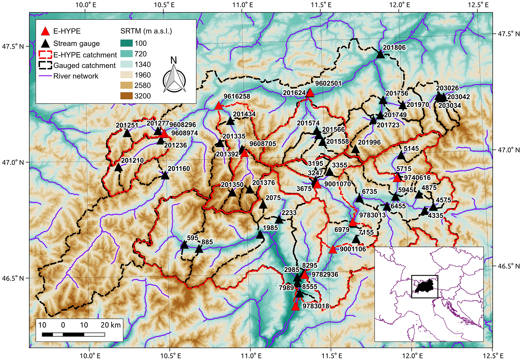
Figure 3Study area: Tyrol. Catchment boundaries for 11 E-HYPE prediction nodes (red) and 46 stream gauges (black).
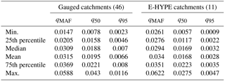
Table 1Study catchments: streamflow properties standardized by drainage area (m3 s−1 km−2) for either gauged catchments or E-HYPE catchments, mean annual flow (qMAF), and 50 % and 95 % streamflow quantiles (q50 and q95, respectively).
3.2 Performance indices
We assessed the performances for predicting regional FDCs by means of Nash–Sutcliffe efficiency (Nash and Sutcliffe, 1970) computed for log-transformed streamflows (LNSEs). These indices are computed as follows:
where Ψ(xj, dk) and , dk) are the empirical and the predicted kth streamflow quantiles at site xj, respectively, μj is the mean of empirical log-transformed streamflow quantiles at site xj, nd is the number of discretization points throughout duration range, and ng is the number of stream gauges.
Another useful metric of performance for the assessment of FDC predictions is the overall absolute curve error (Ganora et al., 2009), which reads as follows:
where Ψ(xj, dk) and , dk) have the same meaning as in Eq. (9).
Similarly, concerning streamflow time series, the assessment of modelled streamflows is carried out with LNSE, but, in this case, it reads as follows:
where Qemp,j(t) and Qmod,j(t) are the empirical and predicted streamflow at site xj and time t, respectively, ωj is the mean of empirical log-transformed streamflow at site xj, ts and np is the number of selected simulation nodes.
Furthermore, we assessed the efficiency of the data-assimilation procedure through the following metric:
LNSEratio quantifies the degree of enhancement of “model 2” relative to “model 1” standardized by the maximum possible improvement (i.e. 1−LNSEmod1). An LNSEratio close to zero means no significant enhancement (detriment of original sequences in case of negative values), whereas an LNSEratio close to 1 indicates that no further enhancement is possible. Such an index is derived from the reciprocal root-mean-squared error ratio between the two models.
Finally, in order to verify whether or not the proposed assimilation procedure GAE-HYPE outperforms rainfall–runoff simulations, for different gauge density scenarios (see Sect. 3.1.3), we used the Wilcoxon signed-rank test with the null hypothesis that simulation model LNSEs are greater than GAE-HYPE ones at 5 % significance level (Hollander and Wolfe, 1999).
4.1 Study region
We focus on a large alpine region located in Tyrol (Italy, Austria and, for small portion only, Switzerland). Our analyses consider two types of data, observed daily streamflows and E-HYPE simulated daily streamflows (see Sect. 4.2), representing different sets of catchments (Fig. 3). In this study, E-HYPE represents the rainfall–runoff model selected to evaluate the procedure presented in Sect. 2.2, which has shown significantly poor results in this region. Indeed, this alpine area is particularly suitable for hydro-power generation, and therefore the presence of dams along the stream network could likely alter the streamflow regime downstream, producing a significant alteration of the natural flow conditions. E-HYPE only simulates the dams present in the global database of GranD (Lehner et al., 2011), which might not be representative for hydropower production at the local scale (Arheimer et al., 2017). Thus, we removed from the initial group of gauged catchments all basins for which the streamflow regime is highly or significantly altered by upstream dams. Table 1 reports the main characteristics of streamflow regimes for 46 gauged basins and 11 selected E-HYPE prediction nodes. Among all E-HYPE prediction nodes available in Tyrol we selected only those whose catchments were the closest to gauged ones, i.e. difference in terms of drainage areas < 14 % and distance between catchment centroids < 15 km. These criteria resulted in the selection of 11 E-HYPE prediction nodes that are evenly distributed in the study region (see red lines in Fig. 3). We addressed the limited differences existing between drainage areas of E-HYPE and gauged basins by adopting the drainage-area ratio technique (Farmer and Vogel, 2013), that is by rescaling daily streamflows according to drainage areas of the corresponding catchment. Such a method assumes the same unit daily streamflow for any pair of hydrologically similar catchments i and j, which reads as follows:
where Qi(t) represents the daily streamflow at day t for catchment i, and Qj(t) is the daily streamflow at day t for catchment j. In our application, i and j could correspond to any given pair (stream gauge, E-HYPE prediction node), and Ai and Aj the corresponding drainage areas. Finally, it is worth pointing out that neither the observed nor the E-HYPE series present zero values in their recording (or simulation) periods for each of the 11 selected nodes.

Figure 4Schematic concept of the HYPE model (all equations are available at http://hypecode.smhi.se/, last access: 30 July 2018).
4.2 Pan-European rainfall–runoff simulation: E-HYPE
The HYdrological Predictions for the Environment (HYPE) model is a hydrological model for small-scale and large-scale assessments of water resources and water quality, developed at the Swedish Meteorological and Hydrological Institute (SMHI) during 2005–2007 (Lindström et al., 2010). The European application, E-HYPE, has been proved to be a powerful tool for water resources managers and practitioners, addressing nutrient concentration in river flow as well as water forecasts on short or seasonal timescale. It is also widely used to estimate snow storage and accumulated TWh (terawatt hour) of water inflow to hydropower dams and in climate change impact analysis (Donnelly et al., 2017). The website Hypeweb (http://hypeweb.smhi.se, last access: 30 July 2018) provides visualization and free downloading of 30 years of continuous and consistent daily streamflow simulations across the European river network at rather fine scale (i.e. the average size of elementary catchments is equal to 215 km2) as well as forecasts and climate change impact analysis.
The HYPE model is open-access and can be downloaded with documentation and model set-up guidelines from the model website (http://hypecode.smhi.se/, last access: 30 July 2018). It simulates water flow and substances on their way from precipitation through soil, river and lakes to the river outlet (Lindström et al., 2010). River basins are divided into sub-basins, which in turn are divided into classes (the finest calculation units) depending on land use, soil type and elevation (Fig. 4).
The soil is modelled as several layers, which may have different thicknesses for each class. In E-HYPE, each sub-basin can have up to some 40 soil and land-use classes, which are lumped within the sub-basins, while the watercourses are routed through the river network. The model parameters can be associated with land use (e.g. evapotranspiration) or soil type (e.g. water content in soil), or be common for the whole catchment or a region with geophysical similarities (Hundecha et al., 2016). This way of coupling the parameters with geographic information makes the model better suited for simulations in ungauged catchments.
The application of the geostatistical method TNDTK through an LOOCV procedure reveals an agreement between empirical values and predictions as shown in Figs. 5 and 6. Specifically, Fig. 5 reports empirical (x axis) against geostatistically predicted (y axis) MAF values as well as LNSEs obtained in cross-validation (i.e. 0.96). Figure 6a shows a scatter diagram between observed (x axis) and predicted streamflows (y axis) from FDCs. This agreement is also confirmed by the distributions of on-site LNSE values (see box plots in Fig. 6b); the median LNSE is equal to 0.97, while mean LNSE is ca. 0.90. The performance obtained in cross-validation legitimizes the use of TNDTK for predicting FDCs in the study area at the 11 E-HYPE prediction nodes of interest, for which TNDTK delivers high prediction capability, with LNSE values above 0.97 (see the spatial distribution of efficiency values in Fig. 10a).
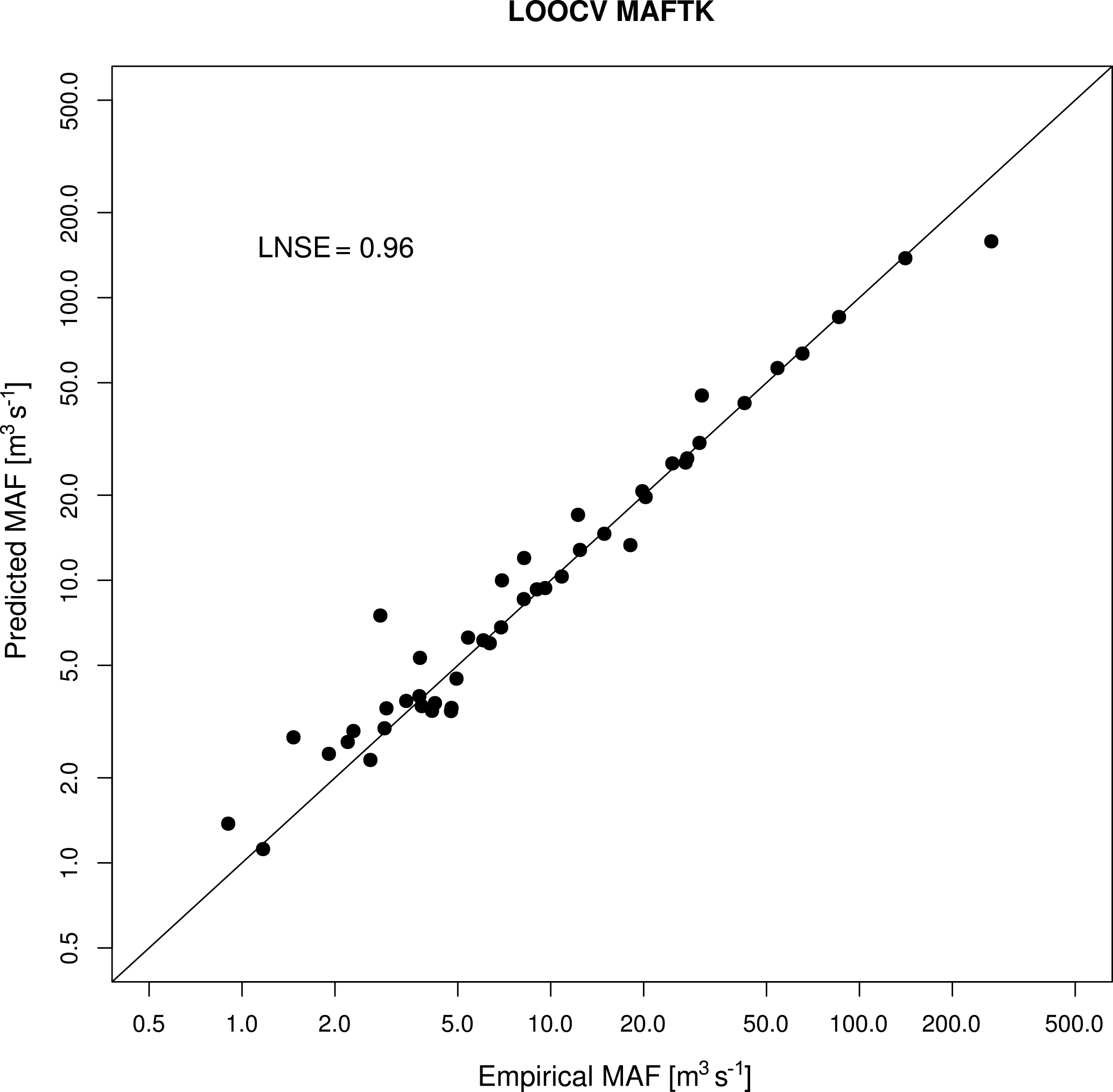
Table 2Nash–Sutcliffe Efficiencies computed on log-transformed daily streamflows for E-HYPE and GAE-HYPE: median values for the 11 prediction nodes considered in the study; smallest enhancement (IDs 3675 – 9001070), largest enhancement (IDs 201236 – 9608296).
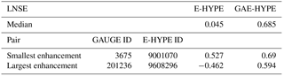
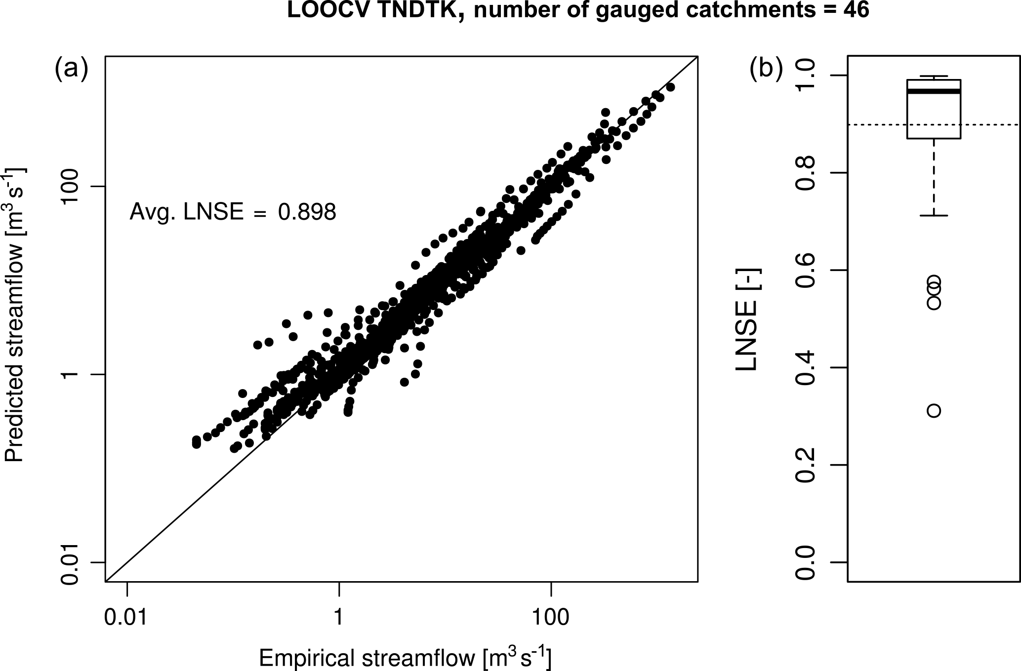
Figure 6(a) Scatter diagrams of empirical (x axis) vs. predicted (y axis) streamflows. (b) Box-plot representation of on-site LNSE values, summarizing the first, second (median) and third quartiles along with whiskers extending to the most extreme non-outlying data point (outliers are highlighted as circles and lay at more than 1.5 times the interquartile-range from the nearest quartile); the average on-site LNSE value is reported in (a) and illustrated as a dashed line in (b).
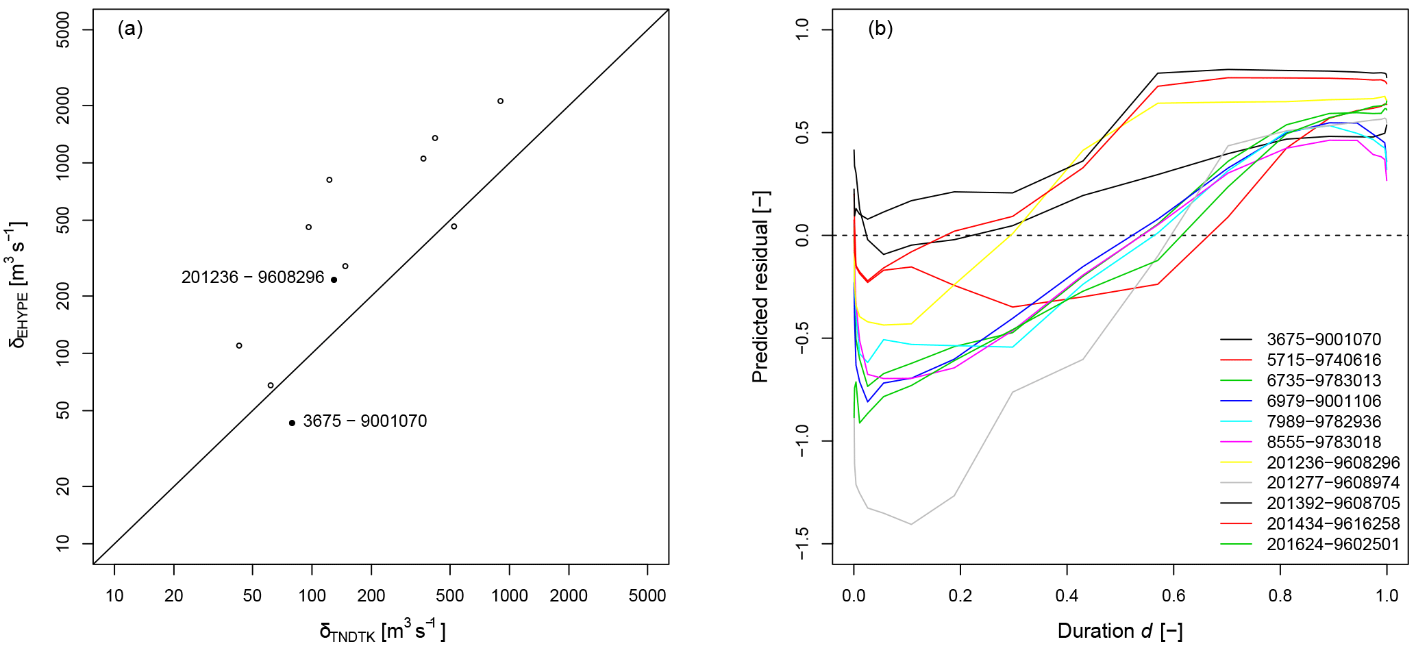
Figure 711 E-HYPE prediction nodes: (a) comparison between TNDTK (x axis) and E-HYPE (y axis) in terms of distances δs between empirical and predicted FDCs; the 1:1 line represents equivalent performance for TNDTK and E-HYPE; (b) standardized residual–duration curves computed as illustrated in Eq. (8) (TNDTK streamflow quantiles are used for standardization).
Figure 7 reports the results obtained by applying the aforementioned cross-validation algorithm. Circles in Fig. 7a represent the cumulative absolute error δ (see Eq. 10) computed for each catchment pair i–j, between empirical FDCs and predicted FDCs for either E-HYPE (δEHYPE on the y axis) or TNDTK (δTNDTK on the x axis) predictions. This figure clearly shows that for 9 out of 11 target sites the geostatistical method TNDTK outperforms E-HYPE in predicting FDCs. Moreover, one of the two sites for which E-HYPE outperforms TNDTK shows nearly the same performance as TNDTK (i.e. the circle is very close to the 1:1 line), while the other one (i.e. site 3675-9001070, highlighted with a black dot in the figure) is associated with the worst performance of TNDTK relative to E-HYPE (see also Sect. 6 on this). Figure 7b reports estimated residual–duration curves (DCs) for the selected sites. For the sake of representation, we report standardized residuals in the y axis, i.e. residuals divided by the corresponding streamflow quantiles predicted via TNDTK; we referred to TNDTK quantiles for standardization since the real empirical FDC is supposed to be unknown (see cross-validation algorithm illustrated in Sect. 3.1.2). Overall, DCs show negative values for lower durations and positive values for higher durations (see also Fig. 8). This means that, in Tyrol, E-HYPE tends to overestimate streamflow in wet periods as well as to underestimate streamflows in drier ones relative to the geostatistically predicted FDCs (i.e. TNDTK, see the left panels in Fig. 8). We eventually used the DC curves, which are estimates of E-HYPE residuals, to assimilate locally available streamflow data into E-HYPE simulated series as illustrated in Fig. 2, obtaining what we termed GAE-HYPE simulations (see right panels of Fig. 8).
Representativeness of simulations (i.e. E-HYPE and GAE-HYPE simulated daily streamflows) is assessed through a Nash–Sutcliffe efficiency of log-flows (LNSE) computed by referring to a recorded streamflow time period of the paired stream gauge (see pairing method adopted in Sect. 4.1). Improvements are obtained with the proposed data-assimilation procedure relative to E-HYPE (Fig. 9). Indeed, we obtained an enhancement of LNSE values of GAE-HYPE simulations relative to the original E-HYPE ones for all the 11 selected sites, which show LNSE increments from −0.462 to 0.594 in the best case (catchment pair IDs: 201236–9608296) and from 0.527 to 0.690 in the worst case (catchment pair IDs: 3675–9001070, see also Table 2). The median on-site LNSE value increases from 0.045 to 0.685, which ultimately underlines the benefits introduced with the proposed method. Figure 9, also, illustrates the impact of geostatistical data assimilation for the two E-HYPE prediction nodes mentioned above (i.e. the one characterized by the best improvements in terms of overall LNSE value, and the one associated with the most limited improvement).
Moreover, looking at the spatial distribution of LNSE values across the 11 selected prediction nodes within the study area depicted in Fig. 10, it is clear how the proposed enhancement strategy benefits from the unbiased estimations of FDCs. In fact, TNDTK shows homogeneous and rather high performance for predicting FDCs (Fig. 10a); also, Fig. 10b and c reveal that the enhancement capabilities of the assimilation procedure are lower for those catchments where E-HYPE performs better (see elementary catchments filled in yellow to green in Fig. 10), whereas the assimilation procedure proves to be powerful when E-HYPE performs worse (see elementary catchments coloured in orange to red), bringing efficiencies from negative to positive values in all cases (from green to blue).

Figure 8Examples of comparison between observed streamflow series (black dashed lines) and simulated daily streamflows via E-HYPE (red solid lines) and GAE-HYPE (blue solid lines) for two representative sites and a given year, showing two cases for which the geostatistical assimilation procedure resulted in sizeable (a) and limited (b) improvements, respectively.
The assessment of gauge density impacts on the proposed procedure reveals that enhancements are obtained even with the lowest gauge density scenario (i.e. seven gauging stations). Figure 11 displays a clear pattern, showing an improvement in the degree of enhancement associated with an increasing gauge density. Moreover, Fig. 11 shows how the degree of enhancement flattens out in cases in which there are more than approximately 25 gauges available per 10 000 km2. Finally, the p values resulting from the Wilcoxon signed-rank tests (see Sect. 3.2) highlight that the assimilation procedure outperforms E-HYPE: the null hypothesis is rejected, with p values always lower than 0.04 %, regardless of the particular stream gauge density scenario.
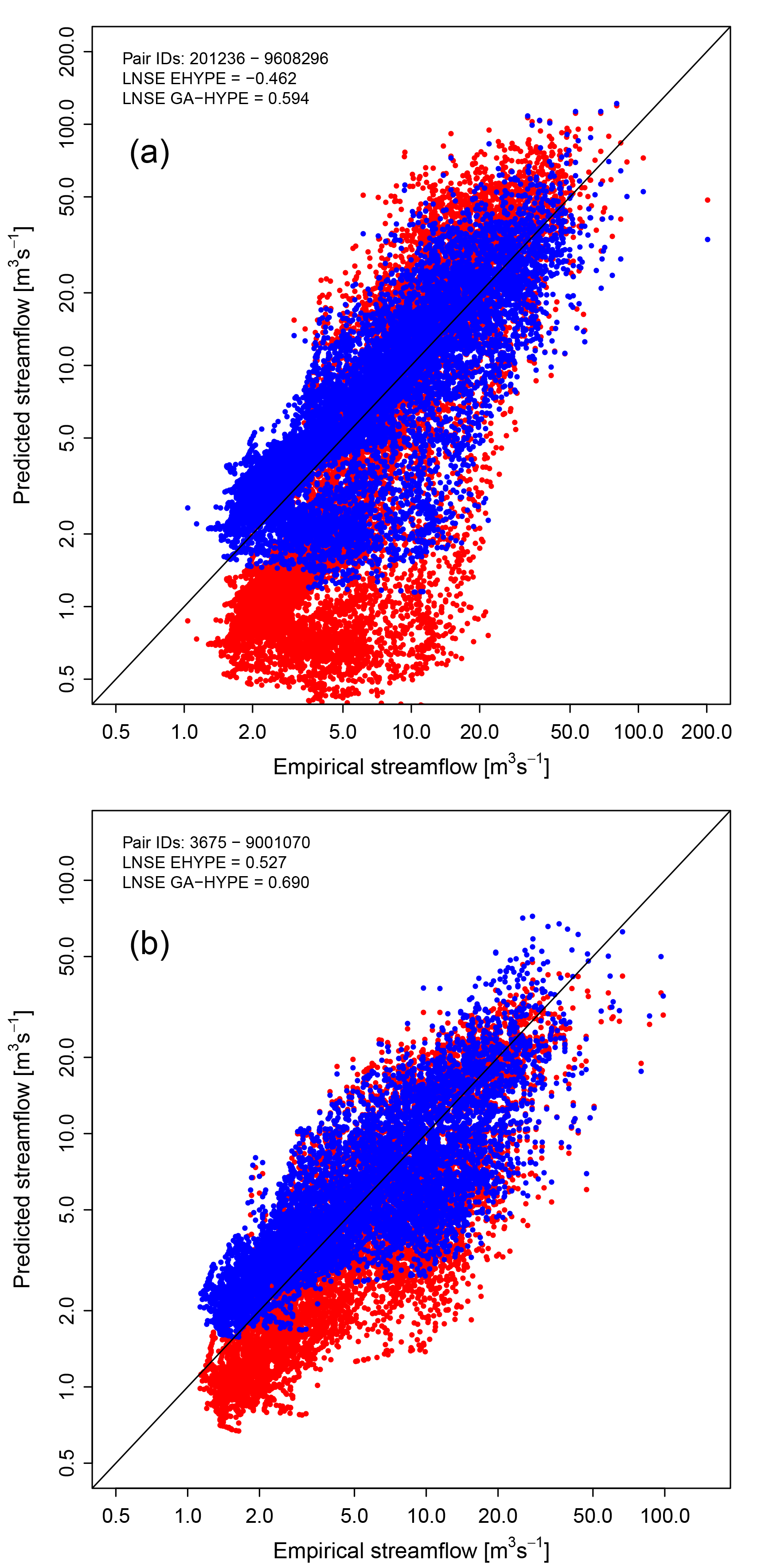
Figure 9Scatter diagrams of empirical vs. simulated daily streamflows for either E-HYPE (red dots) and GAE-HYPE (blue dots) for two representative sites, showing the cases in which the data-assimilation procedure respectively produced the largest (a) and smallest (b) degree of enhancement for the study area, respectively.
This new geostatistical procedure enables practitioners and water resources managers and planners to profit from the wealth of hydrological information, by adjusting open-data products with local observations. We enhanced the streamflow series simulated by macro- and continental-scale rainfall–runoff models at ungauged prediction nodes by assimilating streamflow observations, which are locally available in the region of interest, without having to redo the original hydrological model calculations. This is a recurrent condition since local streamflow data are released under different license terms and policies: some of them could be public and open-access, while some others might not be openly and freely accessible by the broad public. The E-HYPE model obviously lacks storage capacity in the Tyrol region and the proposed approach to enhance the results should be seen as temporary until a new model version accounting for this is available. We do not propose the procedure as a general fix for structurally unsuitable (Beven and Binley, 1992) models, which have been proved to be unfit for either the area of interest or the water problem at hand. For a more sustainable solution, we suggest using another model structure or re-calibrating the model, instead of post-processing the output. However, this procedure makes sense for making a first assessment of water issues in regions where information is otherwise missing, but only macro-scale models are readily available.
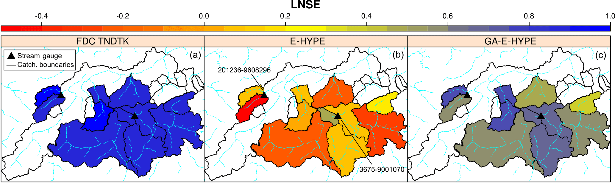
Figure 10Spatial distribution of Nash–Sutcliffe efficiency computed for log-transformed streamflows (LNSEs) at the 11 E-HYPE prediction nodes considered in the study: geostatistically predicted flow–duration curves (FDC TNDTK, a); predicted daily streamflow time series (E-HYPE, b, and GAE-HYPE, c, respectively); the locations of the two sites considered in Figs. 9 and 8 are highlighted with black triangles.
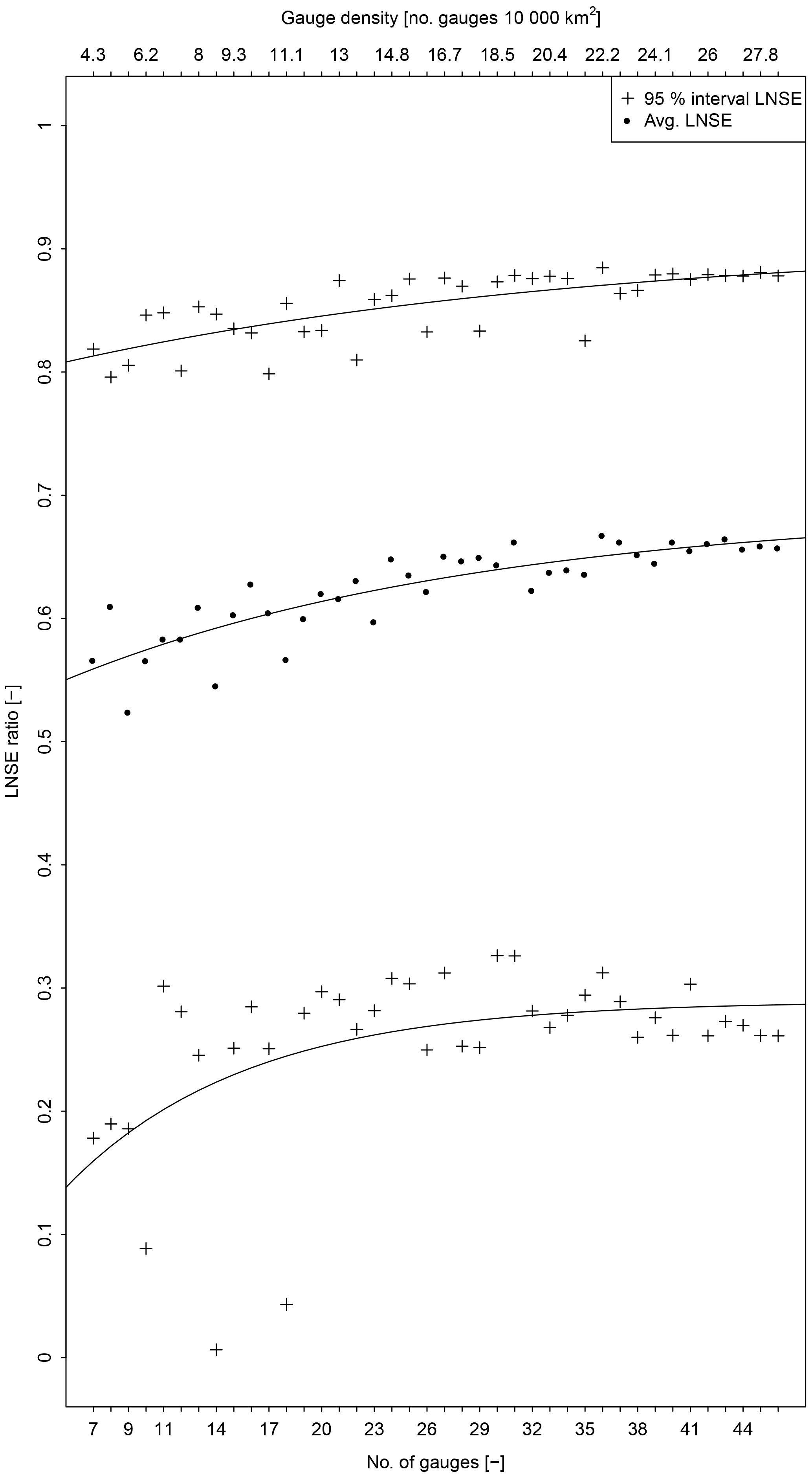
Figure 11LNSE ratio (see Eq. 12) as a function of stream gauge availability: black dots represent the average of 11 LNSE ratio values, while crosses indicate their 95 % confidence interval.
Our study shows for Tyrol that it is possible to significantly enhance rainfall–runoff simulations resulting from macro-scale, regional or continental hydrological models by geostatistically assimilating (geographically sparse) streamflow observations (see e.g. Figs. 8, 9 and 10); provided that available streamflow series are long enough to obtain a good empirical approximation of the long-term FDC for the site of interest (Castellarin et al., 2013). Indeed, series length of the observed streamflow dataset controls the magnitude of duration extremes (i.e. duration boundary interval), which, in turn, might affect the adopted resampling scheme needed for predicting FDCs at simulation nodes. Nonetheless, in some specific application, very high or very low durations might be of particular interest (e.g. studies focused on flood or drought only); therefore a preliminary investigation on the resampling scheme (e.g. duration extremes, duration intervals, resolution of the points to represent correctly the whole curve) should always be taken into account.
One of the main advantages of the proposed method is that the end user can get enhanced streamflow simulations without any further model calibration or refinement. Even though one could argue that when additional streamflow data become available at neighbouring gauges it should be used for improving the performance of the model at the site of interest, calibrating and validating macro-scale and regional model could be a time-consuming and computationally demanding task. The proposed procedure, instead, is neither computational nor data-intensive, and is implemented only using observed streamflow data and a GIS vector layer with catchment boundaries (see e.g. Fig. 3). The application requires the identification of a suitable regional model for predicting FDC in ungauged basis (see e.g. Fig. 6). However, it has advantages, such as (a) a regional model can be a very informative and useful tool for water resources managers and planners, and (b) the subsequent advantages obtained from the data-assimilation procedure is transferred downstream in the entire regional river network (see Fig. 11).
One important limitation of the proposed method is that, once a target prediction node is considered, any given simulated streamflow value is associated with a single duration, which corresponds to a particular estimated residual, which will be used in turn for correcting the streamflow value itself (see Figs. 2 and 8). Essentially, this means that the volumes from E-HYPE are discarded while the sequencing of E-HYPE simulations is retained. Moreover, this algorithm cannot possibly account for seasonal (or interannual) modifications in the hydrological behaviour of the catchment. Indeed, as shown in the time series comparison in Fig. 8, when the geostatistical prediction of FDCs is unreliable, the assimilation procedure reflects such low accuracy (i.e. the procedure fails to correctly capture high-flow and low-flow regimes; see e.g. the resulting FDC from GAE-HYPE simulations at the catchment pair 3675–9001070 in Fig. 8), propagating this bias throughout the whole simulated series. Finally, designing a theoretical framework that combines statistical data-driven approaches with deterministic process-driven ones is seen by many as the correct way for tackling the “prediction in ungauged basins” (PUB) problem and further advancing the scientific research in this area (Di Prinzio et al., 2011). We believe that our geostatistical data-assimilation procedure for macro-scale hydrological models is one example in this direction. Future analyses will focus on the relaxation of the main limitation of the approach (i.e. the incorporation of seasonal patterns in a data-assimilation procedure) and on the extension of its applicability to anthropologically altered streamflow regimes.
This research work focuses on the development of an innovative method for enhancing streamflow series simulated by macro-, continental-, and global-scale rainfall–runoff models by means of a geostatistical prediction of model residuals. We focus on Tyrol as study region and E-HYPE (European-HYdrological Predictions for the Environment, from the Swedish Meteorological and Hydrological Institute, SMHI) as a macro-scale hydrological model; nevertheless, the geostatistical data-assimilation procedure is general and can be applied to simulated streamflow series coming from other macro-scale rainfall–runoff models. The proposed data-assimilation procedure utilizes streamflow data that are locally available for the area of interest, which were not considered in the implementation of the macro-scale hydrological model; it (1) adopts top-kriging for regionally interpolating empirical period-of-record flow–duration curves (FDCs) that can be constructed from locally available streamflow data; (2) constructs residual–duration relationships at any prediction node in the study region where simulated streamflow series are available, by comparing FDCs resulting from geostatistical interpolation (top-kriging) and rainfall–runoff simulation (E-HYPE); and (3) uses the residual–duration curve to enhance macro-scale simulated streamflows.
The cross-validation tests of the proposed approach with different scenarios of streamflow data availability show the significant advantages of geostatistical data assimilation even for very low stream-gauging network densities (i.e. ca. 1 gauge per 2000 km2). It can become a stand-alone numerical tool to be used for enhancing results from macro-scale models anywhere along the stream network of a given region. Potential applications are envisaged for a variety of water resources management and planning problems that require accurate streamflow series (e.g. regional assessment of hydropower potential, habitat suitability studies, surface water allocation, civil protection management strategies, climate change trends, safety of river structures). Future analyses will address the main limitation of the proposed geostatistical data-assimilation procedure, aiming to incorporate observed seasonal and inter-annual variations of the hydrological behaviour of the study region as well as other hydrological features (e.g. baseflow index or peak-flow data) into the geostatistical regionalization of model residuals.
The analysis was carried out in the Virtual Water Science Lab developed within the FP7 funded research project SWITCH-ON (grant agreement no. 603587). We invite the interested reader to explore the experiment protocol here: http://dl-ng005.xtr.deltares.nl/view/462/ (Pugliese et al., 2017).
AP performed the numerical analyses, data handling and homogenization. SP contributed to the algorithm coding. AC, AP, AM, SP, BA, RC, GB, and JP had an essential role in designing the framework of the analysis, developing methods and testing procedures, while SB and PM contributed to large dataset pre-processing. All authors made a substantial contribution to the critical interpretation of results and provided important ideas to further improve the study. All authors actively took part in drafting, writing, and revising the paper.
The authors declare that they have no conflict of interest.
The analyses presented in the study are the main outcomes of the
international experiment Geostatistical enhancement of European hydrological
predictions (GEEHP), which was performed in the Virtual Water-Science Lab
developed within the European Commission FP7 funded research project
SWITCH-ON (Sharing Water-related Information to Tackle Changes in the
Hydrosphere – for Operational Needs, grant agreement no. 603587). The
overall aim of the project is to promote data sharing to exploit open data
sources. The study also contributes to developing the framework of the
“Panta Rhei” Research Initiative of the International Association of
Hydrological Sciences (IAHS).
Edited by: Fuqiang Tian
Reviewed by: Three anonymous referees
Alcamo, J., Döll, P., Henrichs, T., Kaspar, F., Lehner, B., Rösch, T., and Siebert, S.: Development and testing of the WaterGAP 2 global model of water use and availability, Hydrolog. Sci. J., 48, 317–337, https://doi.org/10.1623/hysj.48.3.317.45290, 2003. a
Alfieri, L., Burek, P., Dutra, E., Krzeminski, B., Muraro, D., Thielen, J., and Pappenberger, F.: GloFAS – global ensemble streamflow forecasting and flood early warning, Hydrol. Earth Syst. Sci., 17, 1161–1175, https://doi.org/10.5194/hess-17-1161-2013, 2013. a
Archfield, S. A., Pugliese, A., Castellarin, A., Skøien, J. O., and Kiang, J. E.: Topological and canonical kriging for design flood prediction in ungauged catchments: an improvement over a traditional regional regression approach?, Hydrol. Earth Syst. Sci., 17, 1575-1588, https://doi.org/10.5194/hess-17-1575-2013, 2013. a
Archfield, S. A., Clark, M., Arheimer, B., Hay, L. E., McMillan, H., Kiang, J. E., Seibert, J., Hakala, K., Bock, A., Wagener, T., Farmer, W. H., Andréassian, V., Attinger, S., Viglione, A., Knight, R., Markstrom, S., and Over, T.: Accelerating advances in continental domain hydrologic modeling, Water Resour. Res., 51, 10078–10091, https://doi.org/10.1002/2015WR017498, 2015. a
Arheimer, B., Wallman, P., Donnelly, C., Nyström, K., and Pers, C.: E-HypeWeb: Service for Water and Climate Information – and Future Hydrological Collaboration across Europe?, in: Environmental Software Systems. Frameworks of eEnvironment, IFIP Advances in Information and Communication Technology, Springer, Berlin, Heidelberg, 657–666, https://doi.org/10.1007/978-3-642-22285-6_71, 2011. a
Arheimer, B., Donnelly, C., and Lindström, G.: Regulation of snow-fed rivers affects flow regimes more than climate change, Nat. Commun., 8, 62, https://doi.org/10.1038/s41467-017-00092-8, 2017. a, b
Beck, H. E., van Dijk, A. I. J. M., de Roo, A., Miralles, D. G., McVicar, T. R., Schellekens, J., and Bruijnzeel, L. A.: Global-scale regionalization of hydrologic model parameters, Water Resour. Res., 52, 3599–3622, https://doi.org/10.1002/2015WR018247, 2016. a
Beven, K. and Binley, A.: The future of distributed models: Model calibration and uncertainty prediction, Hydrol. Process., 6, 279–298, https://doi.org/10.1002/hyp.3360060305, 1992. a
Blöschl, G., Sivapalan, M., Thorsten, W., Viglione, A., and Savenije, H.: Runoff prediction in ungauged basins: synthesis across processes, places and scales, Cambridge University Press, Cambridge, 2013. a
Castellarin, A.: Regional prediction of flow-duration curves using a three-dimensional kriging, J. Hydrol., 513, 179–191, https://doi.org/10.1016/j.jhydrol.2014.03.050, 2014. a, b, c
Castellarin, A., Botter, G., Hughes, D. A., Liu, S., Ouarda, T. B. M. J., Parajka, J., Post, M., Sivapalan, M., Spence, C., Viglione, A., and Vogel, R.: Prediction of flow duration curves in ungauged basins, in: chap. 7, Cambridge University Press, Cambridge, 135–162, 2013. a, b, c
Castellarin, A., Persiano, S., Pugliese, A., Aloe, A., Skøien, J. O., and Pistocchi, A.: Prediction of streamflow regimes over large geographical areas: interpolated flow–duration curves for the Danube region, Hydrolog. Sci. J., https://doi.org/10.1080/02626667.2018.1445855, 63, 845–861, 2018. a, b
Castiglioni, S., Castellarin, A., and Montanari, A.: Prediction of low-flow indices in ungauged basins through physiographical space-based interpolation, J. Hydrol., 378, 272–280, https://doi.org/10.1016/j.jhydrol.2009.09.032, 2009. a
Castiglioni, S., Castellarin, A., Montanari, A., Skøien, J. O., Laaha, G., and Blöschl, G.: Smooth regional estimation of low-flow indices: physiographical space based interpolation and top-kriging, Hydrol. Earth Syst. Sci., 15, 715–727, https://doi.org/10.5194/hess-15-715-2011, 2011. a
Cressie, N. A. C.: Statistics for spatial data, Wiley series in probability and mathematical statistics: Applied probability and statistics, J. Wiley, New York, USA, ISBN: 978-0-471-00255-0, 1993. a, b
de Paiva, R. C. D., Buarque, D. C., Collischonn, W., Bonnet, M.-P., Frappart, F., Calmant, S., and Bulhões Mendes, C. A.: Large-scale hydrologic and hydrodynamic modeling of the Amazon River basin, Water Resour. Res., 49, 1226–1243, https://doi.org/10.1002/wrcr.20067, 2013. a, b
De Roo, A. P. J., Wesseling, C. G., and Van Deursen, W. P. A.: Physically based river basin modelling within a GIS: the LISFLOOD model, Hydrol. Process., 14, 1981–1992, https://doi.org/10.1002/1099-1085(20000815/30)14:11/12<1981::AID-HYP49>3.0.CO;2-F, 2000. a
Di Prinzio, M., Castellarin, A., and Toth, E.: Data-driven catchment classification: application to the pub problem, Hydrol. Earth Syst. Sci., 15, 1921–1935, https://doi.org/10.5194/hess-15-1921-2011, 2011. a
Donnelly, C., Andersson, J. C. M., and Arheimer, B.: Using flow signatures and catchment similarities to evaluate the E-HYPE multi-basin model across Europe, Hydrolog. Sci. J., 61, 255–273, https://doi.org/10.1080/02626667.2015.1027710, 2016. a, b, c
Donnelly, C., Greuell, W., Andersson, J., Gerten, D., Pisacane, G., Roudier, P., and Ludwig, F.: Impacts of climate change on European hydrology at 1.5, 2 and 3 degrees mean global warming above preindustrial level, Climatic Change, 143, 13–26, https://doi.org/10.1007/s10584-017-1971-7, 2017. a
Falter, D., Dung, N., Vorogushyn, S., Schröter, K., Hundecha, Y., Kreibich, H., Apel, H., Theisselmann, F., and Merz, B.: Continuous, large-scale simulation model for flood risk assessments: proof-of-concept, J. Flood Risk Manage., 9, 3–21, https://doi.org/10.1111/jfr3.12105, 2016. a
Farmer, W. H.: Ordinary kriging as a tool to estimate historical daily streamflow records, Hydrol. Earth Syst. Sci., 20, 2721–2735, https://doi.org/10.5194/hess-20-2721-2016, 2016. a
Farmer, W. H. and Vogel, R. M.: Performance-weighted methods for estimating monthly streamflow at ungauged sites, J. Hydrol., 477, 240–250, https://doi.org/10.1016/j.jhydrol.2012.11.032, 2013. a
Ganora, D., Claps, P., Laio, F., and Viglione, A.: An approach to estimate nonparametric flow duration curves in ungauged basins, Water Resour. Res., 45, W10418, https://doi.org/10.1029/2008WR007472, 2009. a
Haag, I. and Luce, A.: The integrated water balance and water temperature model LARSIM-WT, Hydrol. Process., 22, 1046–1056, https://doi.org/10.1002/hyp.6983, 2008. a
Habets, F., Boone, A., Champeaux, J. L., Etchevers, P., Franchistéguy, L., Leblois, E., Ledoux, E., Le Moigne, P., Martin, E., Morel, S., Noilhan, J., Quintana Seguí, P., Rousset-Regimbeau, F., and Viennot, P.: The SAFRAN-ISBA-MODCOU hydrometeorological model applied over France, J. Geophys. Res., 113, D06113, https://doi.org/10.1029/2007JD008548, 2008. a
Hjerdt, N., Arheimer, B., Lindström, G., Westman, Y., Falkenroth, E., and Hultman, M.: Going Public with Advanced Simulations, in: Environmental Software Systems. Frameworks of eEnvironment: Proceedings 9th IFIP WG 5.11 International Symposium, ISESS 2011, 27–29 June 2011, Brno, Czech Republic, edited byL Hřebíček, J., Schimak, G., and Denzer, R., Springer, Berlin, Heidelberg, 574–580, https://doi.org/10.1007/978-3-642-22285-6_62, 2011. a, b
Hollander, M. and Wolfe, D. A.: Nonparametric Statistical Methods, Wiley, New York, USA, 1999. a
Hundecha, Y., Arheimer, B., Donnelly, C., and Pechlivanidis, I.: A regional parameter estimation scheme for a pan-European multi-basin model, J. Hydrol.: Reg. Stud., 6, 90–111, https://doi.org/10.1016/j.ejrh.2016.04.002, 2016. a, b
Isaaks, E. H. and Srivastava, R. M.: An Introduction to Applied Geostatistics, Oxford University Press, New York, USA, ISBN: 0195050134, 1990. a
Kim, D., Jung, I. W., and Chun, J. A.: A comparative assessment of rainfall–runoff modelling against regional flow duration curves for ungauged catchments, Hydrol. Earth Syst. Sci., 21, 5647–5661, https://doi.org/10.5194/hess-21-5647-2017, 2017. a
Komma, J., Reszler, C., Blöschl, G., and Haiden, T.: Ensemble prediction of floods – catchment non-linearity and forecast probabilities, Nat. Hazards Earth Syst. Sci., 7, 431–444, https://doi.org/10.5194/nhess-7-431-2007, 2007. a
Kouwen, N., Soulis, E., Pietroniro, A., Donald, J., and Harrington, R.: Grouped Response Units for Distributed Hydrologic Modeling, J. Water Resour. Pl. Manage.-ASCE, 119, 289–305, 1993. a
Kroll, C. N. and Song, P.: Impact of multicollinearity on small sample hydrologic regression models, Water Resour. Res., 49, 3756–3769, https://doi.org/10.1002/wrcr.20315, 2013. a
Krysanova, V., Müller-Wohlfeil, D.-I., and Becker, A.: Development and test of a spatially distributed hydrological/water quality model for mesoscale watersheds, Ecol. Model., 106, 261–289, https://doi.org/10.1016/S0304-3800(97)00204-4, 1998. a
Laaha, G., Skøien, J., Nobilis, F., and Blöschl, G.: Spatial Prediction of Stream Temperatures Using Top-Kriging with an External Drift, Environ. Model Assess., 18, 671–683, https://doi.org/10.1007/s10666-013-9373-3, 2013. a
Lehner, B., Liermann, C. R., Revenga, C., Vörösmarty, C., Fekete, B., Crouzet, P., Döll, P., Endejan, M., Frenken, K., Magome, J., Nilsson, C., Robertson, J. C., Rödel, R., Sindorf, N., and Wisser, D.: High-resolution mapping of the world's reservoirs and dams for sustainable river-flow management, Front. Ecol. Environ., 9, 494–502, https://doi.org/10.1890/100125, 2011. a
Lindström, G., Pers, C., Rosberg, J., Strömqvist, J., and Arheimer, B.: Development and testing of the HYPE (Hydrological Predictions for the Environment) water quality model for different spatial scales, Hydrol. Res., 41, 295–319, https://doi.org/10.2166/nh.2010.007, 2010. a, b
Nash, J. and Sutcliffe, J.: River flow forecasting through conceptual models part I – A discussion of principles, J. Hydrol., 10, 282–290, https://doi.org/10.1016/0022-1694(70)90255-6, 1970. a
Pappenberger, F., Stephens, E., Thielen, J., Salamon, P., Demeritt, D., van Andel, S. J., Wetterhall, F., and Alfieri, L.: Visualizing probabilistic flood forecast information: expert preferences and perceptions of best practice in uncertainty communication, Hydrol. Process., 27, 132–146, https://doi.org/10.1002/hyp.9253, 2013. a
Parajka, J., Merz, R., Skøien, J. O., and Viglione, A.: The role of station density for predicting daily runoff by top-kriging interpolation in Austria, J. Hydrol. Hydromech., 63, 228–234, https://doi.org/10.1515/johh-2015-0024, 2015. a
Pechlivanidis, I. G. and Arheimer, B.: Large-scale hydrological modelling by using modified PUB recommendations: the India-HYPE case, Hydrol. Earth Syst. Sci., 19, 4559–4579, https://doi.org/10.5194/hess-19-4559-2015, 2015. a
Pontes, P. R. M., Fan, F. M., Fleischmann, A. S., de Paiva, R. C. D., Buarque, D. C., Siqueira, V. A., Jardim, P. F., Sorribas, M. V., and Collischonn, W.: MGB-IPH model for hydrological and hydraulic simulation of large floodplain river systems coupled with open source GIS, Environ. Model. Softw., 94, 1–20, https://doi.org/10.1016/j.envsoft.2017.03.029, 2017. a
Pugliese, A., Castellarin, A., and Brath, A.: Geostatistical prediction of flow–duration curves in an index-flow framework, Hydrol. Earth Syst. Sci., 18, 3801–3816, https://doi.org/10.5194/hess-18-3801-2014, 2014. a, b, c, d, e, f, g, h, i, j
Pugliese, A., Farmer, W. H., Castellarin, A., Archfield, S. A., and Vogel, R. M.: Regional flow duration curves: Geostatistical techniques versus multivariate regression, Adv. Water Resour., 96, 11–22, https://doi.org/10.1016/j.advwatres.2016.06.008, 2016. a, b, c, d, e
Pugliese, A., Bagli, S., Mazzoli, P., Parajka, J., Arheimer, B., Capell, R., and Castellarin, A.: Geostatistical Enhancement of European Hydrological Predictions (GEEHP): a SWITCH-ON experiment protocol, available at: http://dl-ng005.xtr.deltares.nl/view/462/ (last access: 30 July 2018), 2017. a
Salinas, J. L., Laaha, G., Rogger, M., Parajka, J., Viglione, A., Sivapalan, M., and Blöschl, G.: Comparative assessment of predictions in ungauged basins – Part 2: Flood and low flow studies, Hydrol. Earth Syst. Sci., 17, 2637–2652, https://doi.org/10.5194/hess-17-2637-2013, 2013. a
Sampson, C. C., Smith, A. M., Bates, P. D., Neal, J. C., Alfieri, L., and Freer, J. E.: A high-resolution global flood hazard model, Water Resour. Res., 51, 7358–7381, https://doi.org/10.1002/2015WR016954, 2015. a
Skøien, J. O.: rtop: Interpolation of data with variable spatial support, r package version 0.5–14, http://CRAN.R-project.org/ package=rtop, last access: 30 July 2018. a
Skøien, J. O., Merz, R., and Blöschl, G.: Top-kriging – geostatistics on stream networks, Hydrol. Earth Syst. Sci., 10, 277–287, https://doi.org/10.5194/hess-10-277-2006, 2006. a, b, c, d, e, f
Smakhtin, V. Y. and Masse, B.: Continuous daily hydrograph simulation using duration curves of a precipitation index, Hydrol. Process., 14, 1083–1100, https://doi.org/10.1002/(SICI)1099-1085(20000430)14:6<1083::AID-HYP998>3.0.CO;2-2, 2000. a
Srinivas, V., Tripathi, S., Rao, A. R., and Govindaraju, R. S.: Regional flood frequency analysis by combining self-organizing feature map and fuzzy clustering, J. Hydrol., 348, 148–166, https://doi.org/10.1016/j.jhydrol.2007.09.046, 2008. a
Strömqvist, J., Arheimer, B., Dahné, J., Donnelly, C., and Lindström, G.: Water and nutrient predictions in ungauged basins: set-up and evaluation of a model at the national scale, Hydrolog. Sci. J., 57, 229–247, https://doi.org/10.1080/02626667.2011.637497, 2012. a
Wan Jaafar, W. Z., Liu, J., and Han, D.: Input variable selection for median flood regionalization, Water Resour. Res., 47, W07503, https://doi.org/10.1029/2011WR010436, 2011. a