Precipitation downscaling using a probability-matching approach and geostationary infrared data: an evaluation over six climate regions

Precipitation is one of the most important components of the global water cycle. Precipitation data at high spatial and temporal resolutions are crucial for basin-scale hydrological and meteorological studies. In this study, we propose a cumulative distribution of frequency (CDF)-based downscaling method (DCDF) to obtain hourly 0.05^∘ × 0.05^∘ precipitation data. The main hypothesis is that a variable with the same resolution of target data should produce a CDF that is similar to the reference data. The method was demonstrated using the 3-hourly 0.25^∘ × 0.25^∘ Climate Prediction Center morphing method (CMORPH) dataset and the hourly 0.05^∘ × 0.05^∘ FY2-E geostationary (GEO) infrared (IR) temperature brightness (T_b) data. Initially, power function relationships were established between the precipitation rate and T_b for each 1^∘ × 1^∘ region. Then the CMORPH data were downscaled to 0.05^∘ × 0.05^∘. The downscaled results were validated over diverse rainfall regimes in China. Within each rainfall regime, the fitting functions' coefficients were able to implicitly reflect the characteristics of precipitation. Quantitatively, the downscaled estimates not only improved spatio-temporal resolutions, but also performed better (bias: −7.35–10.35 %; correlation coefficient, CC: 0.48–0.60) than the CMORPH product (bias: 20.82–94.19 %; CC: 0.31–0.59) over convective precipitating regions. The downscaled results performed as well as the CMORPH product over regions dominated with frontal rain systems and performed relatively poorly over mountainous or hilly areas where orographic rain systems dominate. Qualitatively, at the daily scale, DCDF and CMORPH had nearly equivalent performances at the regional scale, and 79 % DCDF may perform better than or nearly equivalently to CMORPH at the point (rain gauge) scale. The downscaled estimates were able to capture more details about rainfall motion and changes under the condition that DCDF performs better than or nearly equivalently to CMORPH.

1 Introduction

Precipitation is a critical component in the global water cycle (Barrett and Martin, 1981; Smith et al., 1998; Tobler, 2004). Precipitation data at spatio-temporal resolutions are favoured mainly for two reasons. First, the poor representativeness and uneven distribution of gauge stations make the data incapable of reflecting the precipitation variation spatially (Hughes, 2006, Collischonn et al., 2008; Javanmard et al., 2010). Second, ground radar systems can provide full coverage spatial data for most regions, but RADAR is very weak in view of the precipitation intensity and is subject to short time series. Moreover, the validation poses a big challenge for hydrological applications (Krajewski and Smith, 2002).

A number of techniques have been developed to estimate or retrieve precipitation (Kidd and Levizzani, 2011). Based on these technologies, precipitation datasets have been produced at various resolutions, including the Global Precipitation Climatology Project (GPCP) (Huffman et al., 1997, 2001, 2009), the Tropical Rainfall Measuring Mission (TRMM) Multi-Satellite Precipitation (TMPA) (Huffman et al., 2007), the Climate Prediction Center morphing method (CMORPH) (Joyce et al., 2004) and the Global Satellite Mapping of Precipitation (GSMaP) (Ushio et al., 2009), especially over the last 20 years. The typical spatial resolution of these products is 0.25^∘ × 0.25^∘ (Dinku et al., 2007; Ebert et al., 2007; Hirpa et al., 2010; Sohn et al., 2010; Bitew and Gebremichael, 2011; Romilly and Gebremichael, 2011; Thiemig et al., 2012; Hu et al., 2014). This coarse resolution generally impedes the applications of the data for basin-scale hydrological and meteorological studies (Mekonnen et al., 2008). A downscaling procedure would therefore be highly necessary to meet the requirements of small-scale (<10 km) applications.

Downscaling approaches were first used to interpolate regional-scale atmospheric predictor variables to point-scale meteorological series (Karl et al., 1990; Wigley et al., 1990; Hay et al., 1991, 1992). Currently, downscaling approaches are well developed and can be categorised into regression methods, weather pattern approaches, stochastic weather generators and limited-area climate modelling (Wilby and Wigley, 1997; Cannon, 2008). Most methods are based on meteorological or climate models, and assume that relationships can be established between atmospheric parameters at disparate temporal and/or spatial scales (Giorgi and Mearns, 1999; Willems and Vrac, 2011; Kenabatho et al., 2012). Downscaling approaches can also be categorised into dynamical methods (using regional climate models to translate large-scale weather evolution into physically consistent evolution at a higher resolution) and statistical methods (based on statistical relationships between the regional climate and large-scale predictor variables) (Schmidli et al., 2006). At present, these methods are generally available to downscale data from general circulation models.

Various downscaling techniques have been developed to improve the resolution of satellite precipitation data. Immerzeel et al. (2009) used an exponential relationship between the 1 km Normalized Difference Vegetation Index (NDVI) and precipitation to downscale TRMM 3B43 precipitation data on the Iberian Peninsula. Jia et al. (2011) used a linear regression relationship between a combination of NDVI and a digital elevation model and precipitation to downscale TRMM 3B43 precipitation data in the Qaidam Basin of China. Duan and Bastiaanssen (2013) used a two-degree polynomial regression model between NDVI and precipitation to downscale TRMM 3B43 precipitation data in the Lake Tana basin, Ethiopia, and the Caspian Sea region, Iran. These studies manifest the potential of downscaling methods to obtain fine-resolution precipitation (<10 km), while mainly focusing on precipitation data with low temporal resolutions (i.e. annual or monthly).

The main objective of this study is to develop a regression-based downscaling method to obtain precipitation estimates with a high spatio-temporal resolution (0.05^∘, hourly). Barrett et al. (1991) proposed a cumulative histogram method to relate precipitation observations to satellite estimates in an effort to avoid bias problems related to simple regression. In this study, we propose a cumulative distribution of frequency (CDF)-based downscaling method (DCDF) and perform preliminary validation using CMORPH and geostationary (GEO) infrared (IR) temperature brightness (T_b) data. This new method can (1) lead to a better understanding of satellite precipitation data and (2) stimulate scientific interests to engender the development of precipitation data with improved resolutions. The following section introduces study areas and datasets. Section 3 introduces the principles, framework and procedure of the downscaling method. Section 4 presents the major findings followed by discussion in Sect. 5. Finally, Sect. 6 concludes.

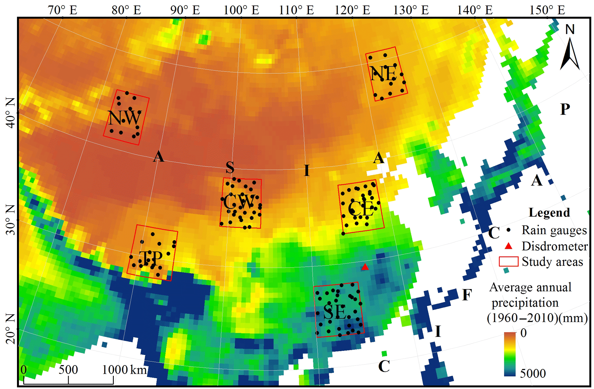
Figure 1 Geographic and climate situations of the six regions. The locations of the rain gauges are superimposed on the map.

2 Study areas and datasets

2.1 Study areas

Existing studies confirmed that the performances of satellite precipitation estimates are highly dependent on the rainfall regime (Arkin et al., 2006; Ebert et al., 2007; Gottschalck et al., 2005), which varies with climate zone, latitude, longitude and elevation. Thus, six 5^∘ × 5^∘ regions were selected for validation (Fig. 1). Their corresponding geographic and climatic characteristics are listed in Table 1. These areas are distributed from south to north and from east to west, and they incorporate most rainfall regimes.

Table 1 Geographic and climatic situations of the six regions in China.

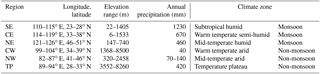
Among the six regions, regions SE (south-east), CE (central-east) and NE (north-east) are located in the eastern monsoon region. It is warm and rainy during the southeast monsoon in June–August, and cold and dry during the northwest monsoon in December–February. These three regions feature low-elevation hills and plains. Regions CW (central-west), NW (north-west) and TP (Tibetan Plateau) are located in the non-monsoon region with a continental climate. CW and NW belong to arid region, with 60–70 % precipitation occurring in June–August. CW has a relatively high elevation, mainly covered by plateaus, mountains and basins. NW is mainly covered by plateaus and basins. TP has a complex climate, mainly covered by plateaus and mountains. The seasonal precipitation distribution has two forms: a unimodal distribution in summer (June–August), and a bimodal distribution in spring (March–May) and autumn (September–November).

2.2 Datasets

2.2.1 Meteorological data

Rain gauge data were obtained from the National Meteorological Information Centre of the China Meteorological Administration (CMA) (http://data.cma.cn/, last access: 10 April 2017). The datasets include daily precipitation records at 137 rain gauge stations in 2014 (Fig. 1). Strict quality control has been applied to check extreme values (Ma, 1998). There are 33, 29, 14, 31, 12 and 18 rain gauges in regions SE, CE, NE, CW, NW and TP, respectively. In the case of more than one station located within a pixel, the rain gauge values are averaged to represent the grid value. Statistical analyses were used to evaluate precipitation estimates at the daily scale. In addition, a disdrometer installed at Xingzi station (29.45^∘ N, 116.05^∘ E) in Jiangxi Province (Fig. 1) provided hourly data in 2014, except June and July when the instrument was subject to a transmission error. Disdrometer data is used to evaluate the precipitation estimates.

2.2.2 Satellite data

IR data (10.7 µm) were collected from the Stretched Visible and Infrared Spin Scan Radiometer (S-VISSR) on board the FY2-E satellite. The data are available at the National Satellite Meteorology Center (http://satellite.nsmc.org.cn/portalsite/default.aspx, last access: 12 August 2017). FY2-E provides hourly coverage of eastern Asia from 75^∘ S to 75^∘ N. The IR T_b data were corrected for zenith angle viewing effects.

CMORPH was developed and produced by the Climate Prediction Center (CPC) in the National Oceanic and Atmospheric Administration (NOAA). CMORPH produces 0.25^∘ × 0.25^∘ 3-hourly global precipitation data using PMW and IR data. PMW data are from the Microwave Imager (TMI) on TRMM, the Special Sensor Microwave Imager (SSM/I) on Defense Meteorological Satellite Program (DMSP) satellites 13–15, the Advanced Microwave Scanning Radiometer Earth Observing System (AMSR-E) on Aqua and the Advanced Microwave Sounding Unit-B (AMSU-B) on NOAA satellite 15–18. Precipitation estimates are generated using the algorithms of Ferraro (1997) for SSM/I, Ferraro et al. (2000) for AMSU-B and Kummerow et al. (2001) for TMI. IR data are obtained from the GEO Operational Environmental Satellites (GOES) 8/10, European Meteorological Satellites (Meteosat) 5/7 and Japanese GEO Meteorological Satellites (GMS) 5. CMORPH uses motion vectors derived from GEO satellite IR imagery to propagate the relatively high-quality precipitation estimates derived from PMW data (Joyce et al., 2004). Hence, quantitative precipitation estimates are based solely on PMW data. GEO-IR data are not used to estimate precipitation but rather to interpolate between two PMW-derived precipitation rate fields.

3 Methodology

3.1 CDF matching

The CDF matching is a probability-based process. It assumes a variable (v) should produce a similar CDF to the reference variable (t). The frequencies of t and v are shown in Eqs. (1)–(2), and the cumulative frequencies in Eqs. (3)–(4).

$$\begin{array}{}\text{(1)}& {\displaystyle }& {\displaystyle }{P}_t=f_{\mathrm{1}}\left(t\right)\text{(2)}& {\displaystyle }& {\displaystyle }{P}_v=f_{\mathrm{2}}\left(v\right)\text{(3)}& {\displaystyle }& {\displaystyle }{C}_t\left(t\right)=\underset{T_{\mathrm{1}}}{\overset{t}{\int }}{f}_{\mathrm{1}}\left(t\right)\text{d}t\text{(4)}& {\displaystyle }& {\displaystyle }{C}_v\left(v\right)=\underset{V_{\mathrm{1}}}{\overset{v}{\int }}{f}_{\mathrm{2}}\left(v\right)\text{d}v\text{(5)}& {\displaystyle }& {\displaystyle }{C}_v^{-\mathrm{1}}\left[C_t\right(t\left)\right]\stackrel{f_{\mathrm{3}}}{⟶}t,\end{array}$$

where P_t and P_v are the probability of t and v, f₁(t) and f₂(v) are probability density functions of t and v and C_t(t) and C_v(v) are the cumulative density functions of t and v, respectively. f₃(v) represents the relationship between t and v.

Figure 2 Schematic of the cumulative distribution of frequency (CDF) matching method.

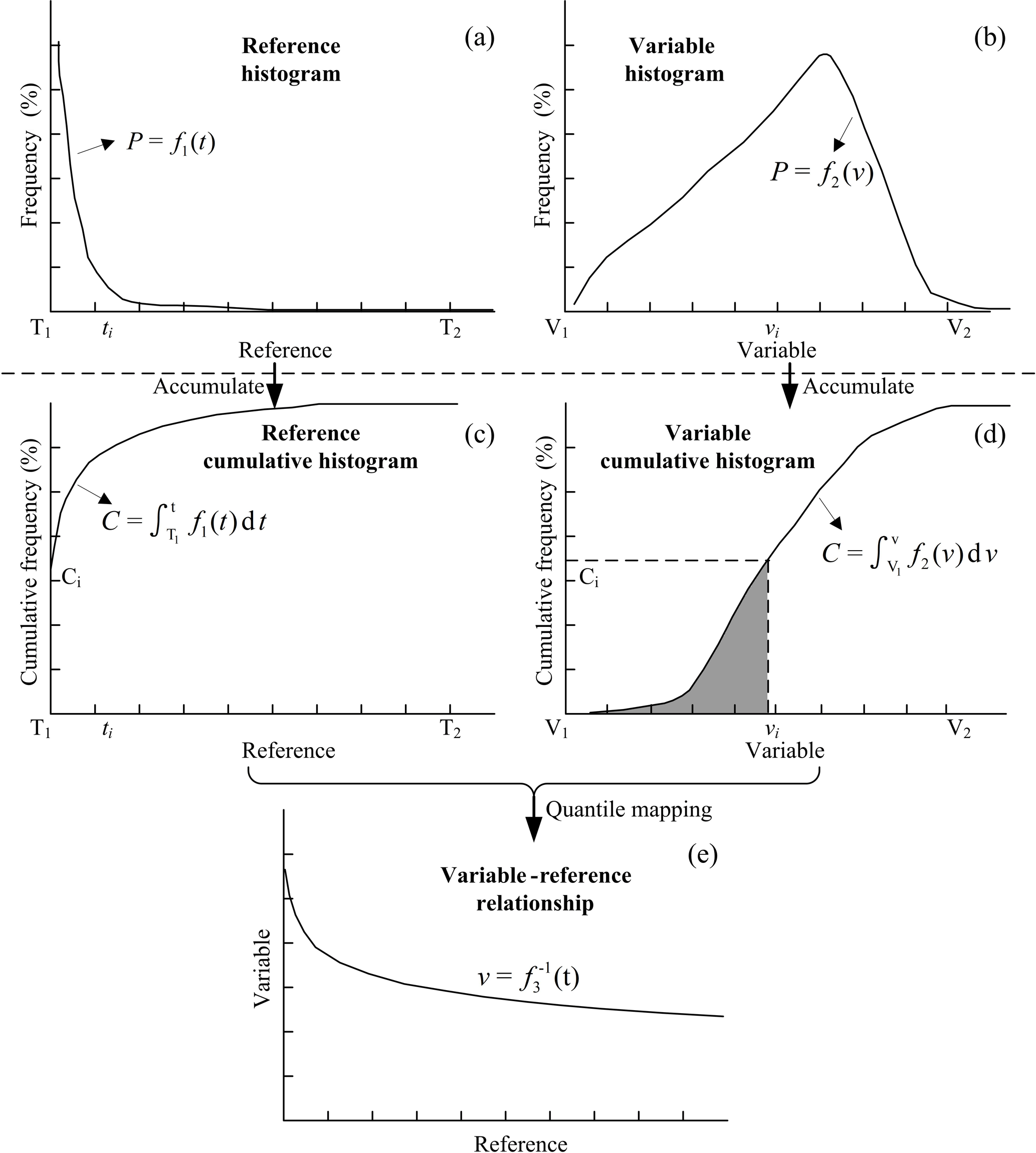
The steps for CDF matching are summarised in Fig. 2. First, t and v are shown in histograms (Fig. 2a, b). The frequency of an arbitrary point t_i (or v_i) on the f₁(t) [or f₂(v)] curve can be expressed as $P(t=t_i)=f_{\mathrm{1}}\left(t_i\right)$ [or $P(v=v_i)=f_{\mathrm{2}}\left(v_i\right)$]. Second, these histograms are transformed into cumulative histograms (Fig. 2c, d). The cumulative frequency of an arbitrary point t_i (or v_i) on the C_t(t) [or C_v(v)] curve can be expressed as $C(t<t_i)={\int }_{T_{\mathrm{1}}}^{t_i}{f}_{\mathrm{1}}\left(t\right)\text{d}t$ [or $C(v<v_i)={\int }_{V_{\mathrm{1}}}^{v_i}{f}_{\mathrm{2}}\left(v\right)\text{d}v$]. Third, these cumulative histograms are matched so that v has a cumulative histogram similar to t. The matching process is implemented by a one-to-one mapping CDF of the variable onto that of the reference (Eq. 5). Last, the v–t relationship is established (Eq. 5) (Fig. 2e). Magnusson et al. (2015) demonstrated that CDF matching works better than a histogram-matching method when low values have high frequencies, which is generally the case for precipitation.

3.2 Downscaling

Our method is based on the work of Barrett et al. (1991) and Kidd and Levizzani (2011). Rainfall can be inferred from IR imagery because heavy rainfall tends to be associated with large, tall clouds with cold cloud tops. Therefore, empirical relationships between the precipitation rate and T_b are derived (Arkin and Meisner, 1987; Greene and Morrissey, 2000; Prigent, 2010). However, these relationships are indirect and exhibit significant variations during the lifetime of a rainfall event. They also differ among rain systems and climatological regimes, which causes large uncertainties in precipitation estimations (Kidd and Levizzani, 2011). Ba and Gruce (2001) demonstrated that a two-degree polynomial model is more effective for describing the relationship, and that the coefficients of the model are region-dependent. Overall, the precipitation–T_b relationship is highly variable over time and space.

Microwave (MW) radiation reflects the physical structures of clouds. Emission from rain droplets increases MW radiation, and scattering by precipitating ice particles decreases MW radiation. Although MW techniques are physically more direct than those based on IR radiation, they can both reflect rainfall events. Therefore, we assume that an IR signal produces a similar frequency distribution of precipitation rates to a MW signal over a certain region during a certain period. Barrett et al. (1991) proposed a cumulative-histogram-matching method to relate rainfall observations to satellite precipitation data. Kidd et al. (2003) applied the same method to estimate rainfall using passive microwave (PMW) and IR data over Africa.

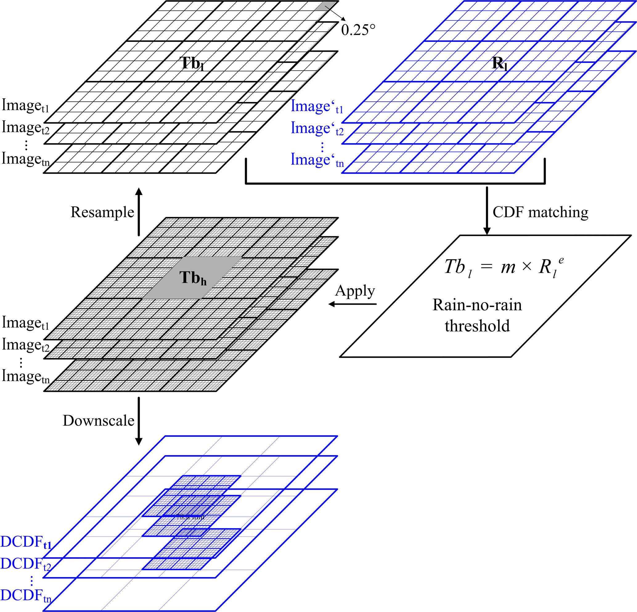
Figure 3 Schematic of the CDF-based downscaling method (DCDF) using CMORPH and FY2-E T_b in this study. R represents the precipitation rate.

The assumptions behind the downscaling method include the following: (1) T_b has a similar cumulative frequency to the precipitation rate at certain spatial and temporal scales, and (2) satellite precipitation products provide relatively accurate estimates with low spatial and temporal resolutions. In contrast, GEO-IR data have a high spatio-temporal resolution, yet low accuracy. Illustrated in Fig. 3, the downscaling method explores the advantages of the satellite precipitation product and GEO-IR data, specifically, (1) to aggregate T_b ($T_{{\text{b}}_{\text{h}}})$ from a high resolution to a low resolution ($T_{{\text{b}}_{\text{l}}})$ similar to the precipitation data (Eq. 6), and (2) to apply the CDF matching to the $T_{{\text{b}}_{\text{l}}}$ and precipitation rate (R_l) to obtain a $T_{{\text{b}}_{\text{l}}}$–R_l relationship and a rain–no-rain threshold (Eq. 7). The downscaled precipitation rates are estimated based on the $T_{{\text{b}}_{\text{l}}}$–R_l relationships (Eq. 8).

$$\begin{array}{}\text{(6)}& {\displaystyle }& {\displaystyle }{T}_{{\text{b}}_{\text{l}}}={\displaystyle \frac{\mathrm{1}}{n}}{\sum }_{i=\mathrm{0}}^n{T}_{{\text{b}}_{\text{h}}}\left(i\right)\text{(7)}& {\displaystyle }& {\displaystyle }{T}_{{\text{b}}_{\text{l}}}=m\times R_{\text{l}}^p\text{(8)}& {\displaystyle }& {\displaystyle }{R}_{\text{h}}=({\displaystyle \frac{T_{{\text{b}}_{\text{h}}}}{m}}{)}^{\mathrm{1}/e},\end{array}$$

where $T_{{\text{b}}_{\text{h}}}$ denotes high-resolution GEO-IR T_b data, $T_{{\text{b}}_{\text{l}}}$ denotes upscaled T_b data, R_l denotes the low-resolution precipitation product, R_h denotes the derived high-resolution estimates, m and e are coefficients of the T_b–R relationship and n is the number of high-resolution pixels within a low-resolution pixel.

Under the assumption that colder clouds are linked to higher rainfall than warmer clouds, the downscaling method assumes a monotonically increasing precipitation rate with decreasing T_b. Therefore, cumulative histograms of the precipitation rate and T_b are matched, so that the occurrence of the heaviest precipitation is associated with the T_b values linked to the heaviest rainfall. Decreasing T_b values are assigned to increasing precipitation rates so that the final distribution of T_b assigned to the precipitation rates is the same as that determined using precipitation rate data. Specially, all precipitation rate (T_b) are sorted in ascending (descending) order. Then both cumulative probability distributions are obtained. The cumulative probability is defined as critical probability when the precipitation rate equals zero. The rain–no-rain threshold is the T_b with a cumulative probability the same as the critical probability. As shown in Fig. 2c and d (T means precipitation rate; V represents T_b), the rain–no-rain threshold is set at about v_i, where the cumulative probability equals C_i (critical probability).

The specific steps used for downscaling with CMORPH and FY2-E IR data are described as follows.

• a.

  Aggregate IR–T_b data ($T_{{\text{b}}_{\mathrm{0.05}}}$) from 0.05 to 0.25^∘ by pixel averaging ($T_{{\text{b}}_{\mathrm{0.25}}}$).
  
  IR–T_b data ($T_{{\text{b}}_{\mathrm{0.05}}}$) were aggregated to a 0.25^∘ grid ($T_{{\text{b}}_{\mathrm{0.25}}})$ for each 3 h period (00:00–03:00, 03:00–06:00, …, 21:00–24:00 UTC), in order to match the spatial and temporal resolutions of CMORPH.

• b.

  Generate the histogram database for CDF matching.
  
  IR–T_b ($T_{{\text{b}}_{\mathrm{0.25}}})$ and the CMORPH precipitation rate (R_0.25) were recorded in a database. The sample area for CDF matching was determined as follows. The horizontal and temporal scales of stratiform precipitation range from 10¹ to 10³ km and from hours to days (Orlanski, 1975; Trapp, 2013), while those of cumuliform precipitation range from a few kilometres to tens of kilometres and from minutes to hours (Orlanski, 1975; Rickenbach, 2008). In combination with previous studies (Kidd et al., 2003; Huffman et al., 2007), the downscaling procedure was conducted at 1^∘ × 1^∘ grids over a 10-day period. To reduce the heterogeneity among grids, a 3 × 3 window was used for smoothing purposes.

• c.

  Build relationships between the precipitation rate and T_b.
  
  The histograms of T_b–precipitation rate were generated and converted to cumulative histograms, and then matched using the CDF matching. (As shown in Fig. 2, the precipitation rate is denoted by T; T_b represents V; v_i is the rain–no-rain threshold.) A power function relationship between the precipitation rate (R_0.25) and T_b ($T_{{\text{b}}_{\mathrm{0.25}}})$ was established for each 1^∘ × 1^∘ area over a 10-day period. Meanwhile, various parameters, including coefficients of the T_b–R relationship, rain–no-rain threshold and R², were obtained.

• d.

  Estimate the precipitation rate pixel by pixel at 1 h and 0.05^∘.
  
  All pixels in the T_b images ($T_{{\text{b}}_{\mathrm{0.05}}})$ were divided into two categories, raining ones below the rain–no-rain threshold and non-raining ones above the threshold. T_b–R relationships were applied to these “raining” pixels. Finally, CMORPH data were downscaled to 1 h and 0.05^∘ × 0.05^∘.

3.3 Variogram

A variogram describes how data correlate with distance. The variogram function γ(h) is defined as half of the mean value of the square of the difference between points separated by a distance h (Matheron, 1963). A variogram is generally an increasing function of distance h. The relationship between γ(h) and h is commonly described using the nugget effect (C₀), sill (C₀+C) and range (D). C₀ denotes micro-scale variations, equated to of γ(0). C₀+C denotes the limit of the variogram γ (+∞). D denotes the distance at which the difference of the variogram from the sill becomes negligible. A variogram is used here to describe the spatial structure of satellite precipitation data.

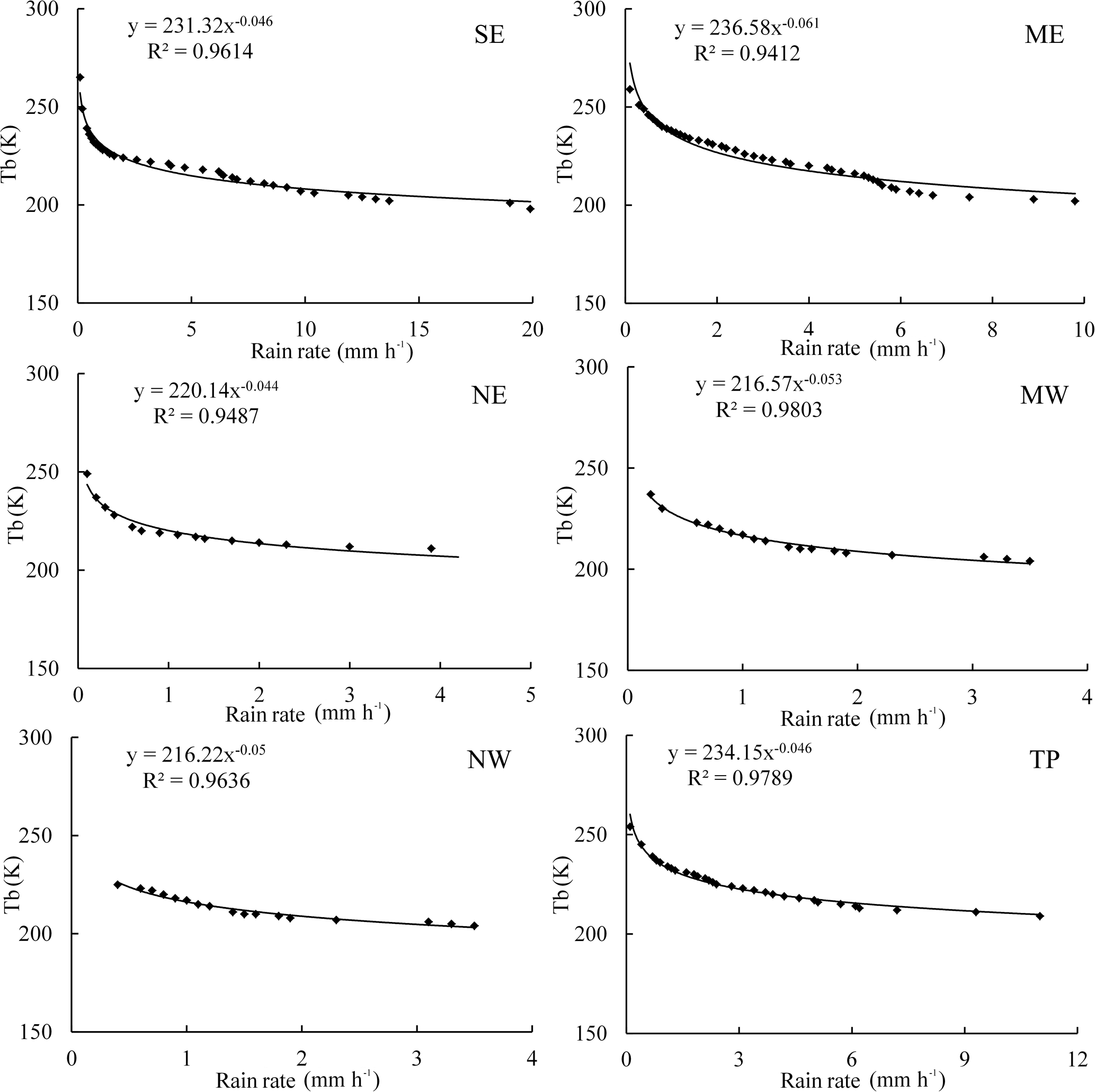
Figure 4 Examples of fitting of the precipitation rate and T_b for each region in China during 9–18 July 2014 for subregion SE (115^∘35^′ E, 27^∘28^′ N), subregion CE (115^∘39^′ E, 36^∘14^′ N), subregion NE (124^∘20^′ E, 51^∘42^′ N), subregion CW (101^∘38^′ E, 37^∘31^′ N), subregion NW (85^∘43^′ E, 46^∘47^′ N) and subregion TP (91^∘06^′ E, 30^∘29^′ N).

4 Results

4.1 T_b–precipitation rate relationship

Figure 4 shows fitting functions between the precipitation rate and T_b within each 1^∘ × 1^∘ grid. It was observed that T_b had a power function relationship with the precipitation rate. With an increase in the precipitation rate, T_b decreased, and the rate of change also reduced. The model fitting R² values were all higher than 0.90. From the region SE to NE, the precipitation rate decreases, mainly subject to latitude. The maximum precipitation rate, rain–no-rain threshold and R² all showed decreasing trends. The maximum precipitation rate was 19.9 mm h⁻¹ in region SE, 9.8 mm h⁻¹ in region CE and 4.3 mm h⁻¹ in region NE. The corresponding T_b values were 198, 202 and 210 K, respectively, and the rain–no-rain threshold values were 265, 259 and 249 K. The probability of the precipitation rate was the largest for a given T_b in region SE, followed by region CE and then region NE. Regions CW and NW are arid, while TP is humid. The maximum precipitation rate was 3.5 mm h⁻¹ for both regions CW and NW and 11 mm h⁻¹ for region TP. The rain–no-rain thresholds for regions CW and NW were approximately 230 K, while it was 254 K for region TP. The probability of the precipitation rate was the largest for a given T_b in region TP because region TP has a complex rain system and high elevation. Generally, the fitting relationships reflected precipitation characteristics well.

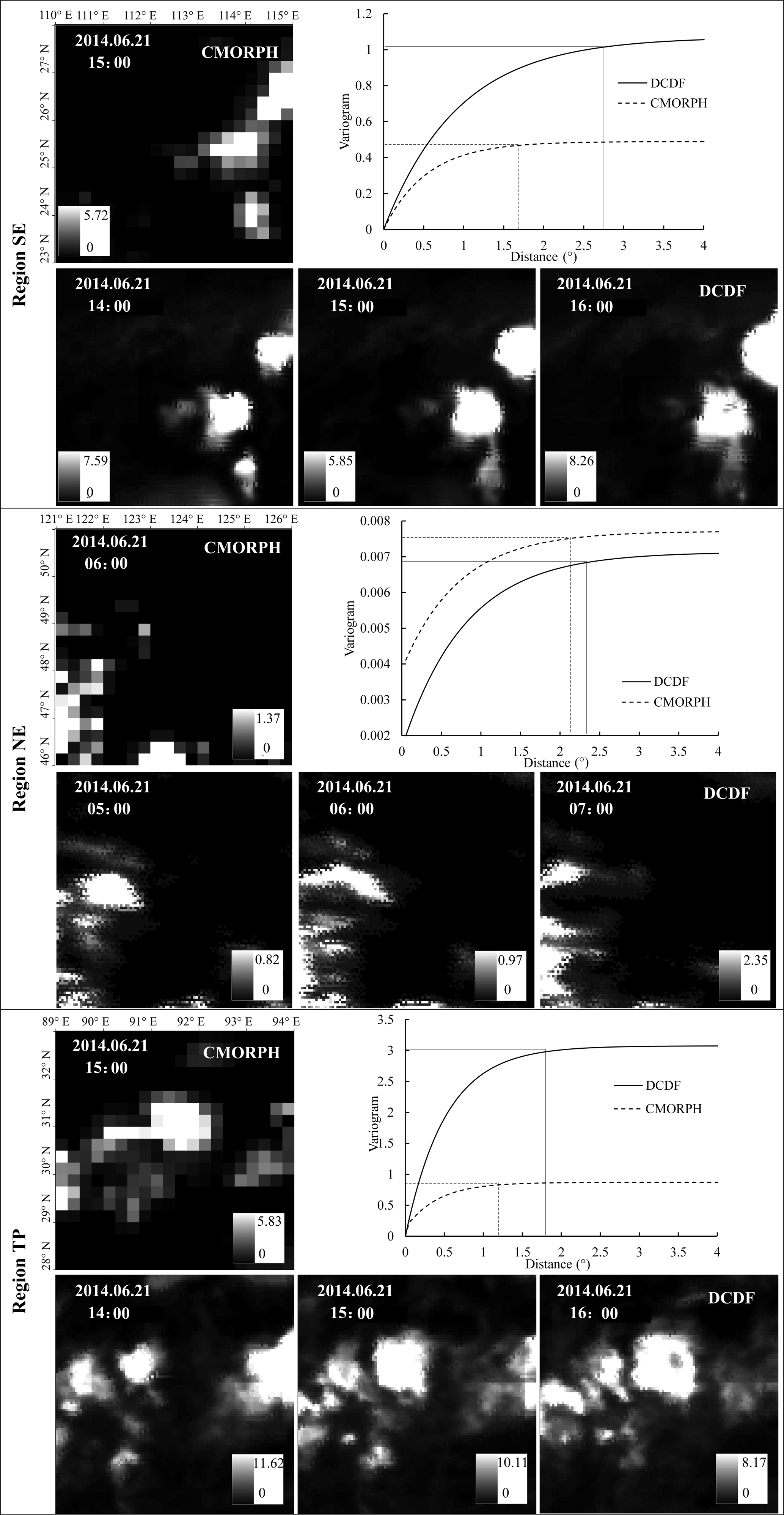
Figure 5 CMORPH precipitation estimates at a nominal resolution of 0.25^∘ and DCDF precipitation maps at a 0.05^∘ resolution for regions SE, NE and TP.

4.2 Estimation results

Figure 5 shows a comparison of the spatial distributions of CMORPH and DCDF precipitation estimates for regions SE, NE and TP. The downscaled precipitation showed a similar spatial distribution to CMORPH, yet it reflected more detailed moving and changing processes of rainfall. To demonstrate clouds captured through DCDF and CMORPH, region SE was exemplified (14:00 to 16:00, 21 June 2014). Three cloud centres were observed in the southeastern and mid-eastern parts at 14:00. One hour later, two centres in the southeast moved eastward and joined together, while another centre moved eastward. Two precipitation centres continued to move eastward at 16:00. In addition, D and sill values of DCDF (2.796 and 1.070) were higher than those of CMORPH (1.614 and 0.489). Large range and sill values indicate a high spatial dependence and high spatial variability. Thus, the spatial dependence and variability for high-resolution data were generally larger than those for low-resolution data.

In region SE, clouds were relatively centralised with a high precipitation rate and were small in size. In region NE, clouds were discrete with a low precipitation rate and were widely distributed. In region TP, both centralised and discrete clouds appeared. Cumuliform cloud is the main type in region SE, while stratiform cloud is dominant in region NE, and both are dominant in region TP. Thus, the cloud distributions obtained through satellite data, especially using the DCDF approach, were consistent with the local characteristics. Sill for cumuliform clouds was larger than that for stratiform clouds. A larger sill value was obtained for region SE (DCDF: 1.070; CMORPH: 0.489) than for region NE (DCDF: 0.007; CMORPH: 0.008). These results indicated that the DCDF method can reflect precipitation characteristics among rain systems and climatological regimes.

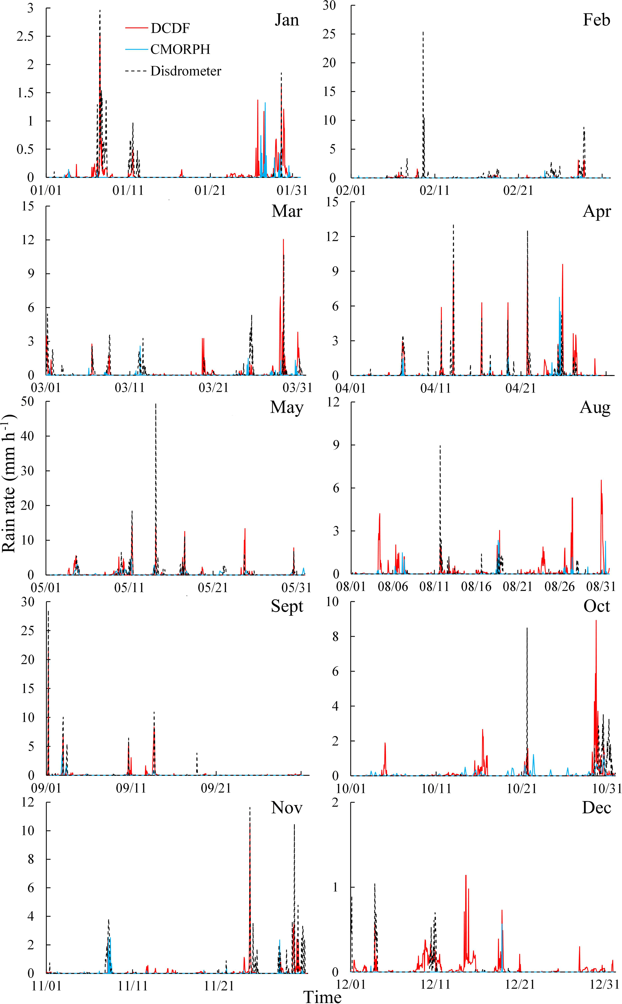
Figure 6 Time series of disdrometer data, original CMORPH and DCDF precipitation at an hourly scale in 2014.

4.3 Validation

Figure 6 shows a comparison among the DCDF, CMORPH and disdrometer at the hourly scale. The DCDF and CMORPH were able to capture rainfall events, although they differed in magnitude from the reference data in some cases. The DCDF effectively reflected the peak of each rainfall event, but could not exactly identify same starting and ending times of rainy events, resulting in somewhat delayed or advanced rainfall. The DCDF may detect non-rainy events as rainy events, especially in dry seasons. CMORPH reported low-rain events as non-rainy events. Both of the DCDF and CMORPH estimates coincided with disdrometer data at precipitation rates ranging from 1 to 10 mm h⁻¹, such as the events from 10:00 to 14:00 on 9 February and from 21:00 on 13 May to 10:00 on 14 May.

Figure 7 Time series of the average precipitation of each region derived from the gauge, DCDF and CMORPH at the daily scale in June 2014.

To demonstrate the performance of the DCDF method, a comparison of the DCDF and CMORPH estimates was conducted at the regional scale and at the point (rain gauge) scale. Figure 7 shows the average precipitation of each region derived from the rain gauge, DCDF and CMORPH. The daily average precipitation over each region showed almost identical temporal variations for DCDF and CMORPH. Both DCDF and CMORPH showed similar temporal patterns to the rain gauge observations, but they were probably subject to overestimation for regions CW and NW and underestimation for regions SE and TP. At the point (gauge) scale, the better fit between DCDF and gauge data than that between CMORPH and gauge data is 10 %. The nearly equivalent fit is 69 %. The poorer fit was mainly evident in regions NW, CW and TP. Figure 8 shows that cases of better fit in the time series of DCDF were generally more consistent with the rain gauge data than CMORPH, although the DCDF series occasionally deviated from gauge data or misreported non-rainy events as rainy events. These results indicated that both DCDF and CMORPH demonstrated nearly equivalent performances at the regional scale, and 79 % DCDF may perform better than or nearly equivalent to CMORPH at the point (gauge) scale.

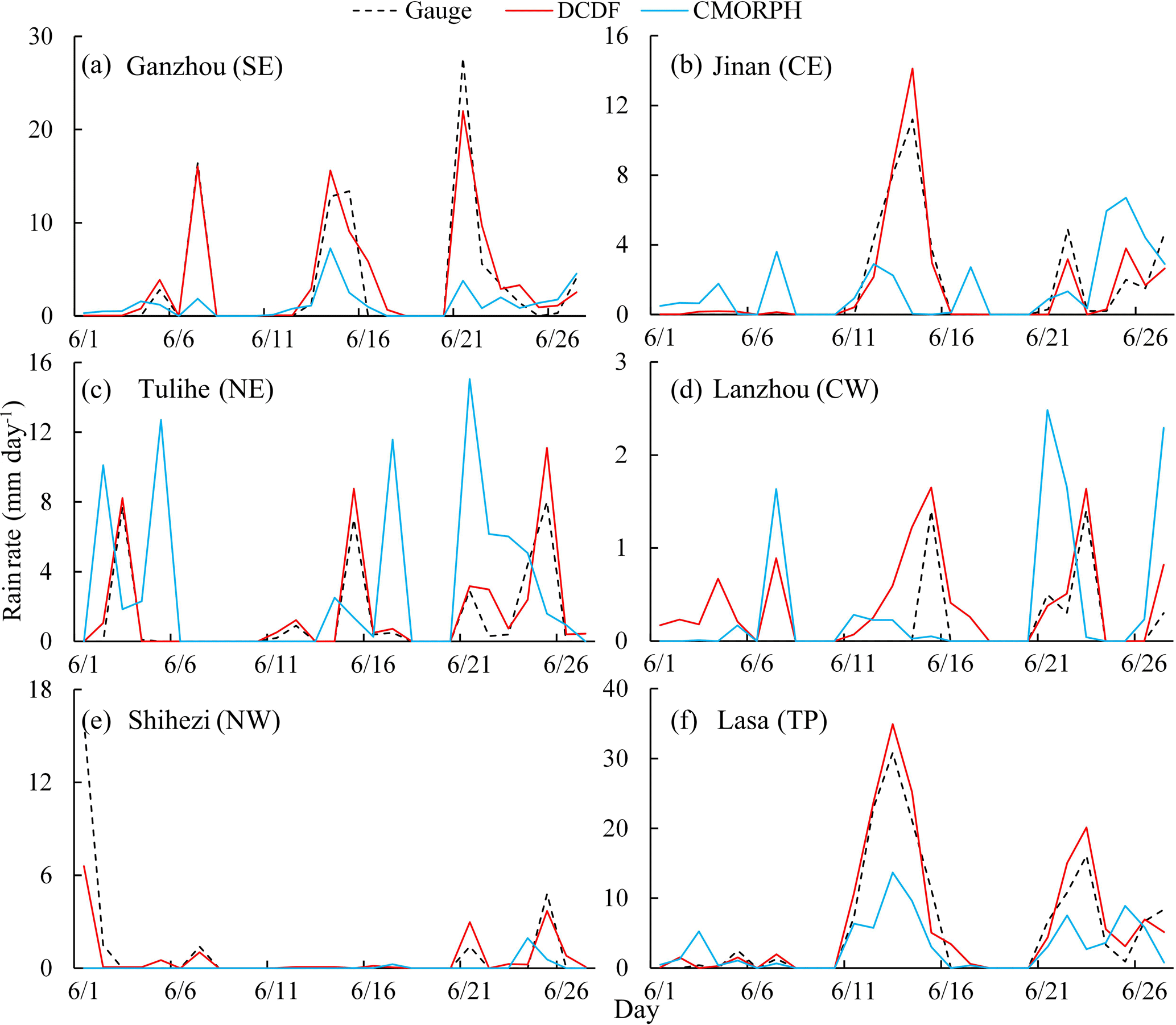
Figure 8 Time series of rain gauge data, original CMORPH and DCDF precipitation for each randomly selected gauge. (a) Ganzhou station (SE): 113.1667^∘ E, 25.8667^∘ N. (b) Jinan station (CE): 117.05^∘ E, 36.6^∘ N. (c) Tulihe station (NE): 121.6833^∘ E, 50.4833^∘ N. (d) Lanzhou station (CW): 103.8833^∘ E, 36.05^∘ N. (e) Shihezi station (NW): 86.05^∘ E, 44.3167^∘ N. (f) Lasa station (TP): 91.1333^∘ E, 29.6667^∘ N.

Table 2 Validation results of the daily precipitation for CMORPH and DCDF in 2014 in the six study regions.

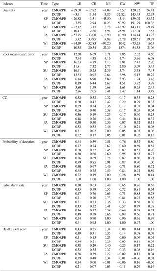
Table 2 lists the seasonal statistics for the six regions at the daily scale. Generally, DCDF performed better than CMORPH in region SE, while it performed equivalently to CMORPH in regions CE and NE. Both of the DCDF and CMORPH showed better performances during the rainy season. The DCDF generally showed the smallest biases between −7.35 and 10.35 % (correlation coefficient, CC: 0.48–0.60) in region SE, and overestimated precipitation by 2.66–33.95 % (CC: 0.05–0.53) in regions CE and NE. CMORPH underestimated precipitation by 20.82–94.19 % (CC: 0.31–0.59) in region SE and showed biases between −93.2 and 6.78 % (CC: 0.00–0.50) in regions CE and NE. DCDF and CMORPH both exhibited poor performances in regions CW, NW and TP, and showed large biases (−73.75–2106 %), low CC values (0.01–0.44) and high false alarm rate (FAR) values (0.33–1.00) during the winter. Further inspection showed that the DCDF overestimation was due to high probability of detection and FAR, which may be caused by a low rain–no-rain threshold. The large biases for regions CW, NW and TP were likely due to the insensitivity of precipitation data to very low precipitation in arid regions and the inability to estimate precipitation over mountainous or hilly areas where orographic rain systems dominate.

5 Discussion

Existing downscaling methods make an assumption that local-scale patterns are driven by large-scale climatic fluctuations (Wilby and Wigley, 1997; Wilby et al., 2002). Most of these methods rely on meteorological or climate models and utilise multiple parameters, such as temperature, humidity, pressure, vorticity and geostrophic airflow. These methods are not used to downscale satellite precipitation products, possibly due to a diversity of parameters and complexity of the meteorological and climate models. In contrast, the DCDF method in this study assumes that the IR retrieval should produce a frequency distribution of precipitation rates similar to that produced by MW retrievals over a certain region during a certain period; that is, IR estimations and MW retrievals from clouds have strong statistical frequency similarities.

Due to high spatial and temporal variability of precipitation, the DCDF method must be conducted over a certain region during a certain period. The area and time period must be large enough for a reasonable sample size, but small enough to represent local characteristics. In the TMPA algorithm, a relationship between IR and the precipitation rate is built within a 1^∘ × 1^∘ area by 3 × 3 windows over the period of a month (Huffman et al. 2007). Kidd et al. (2003) obtained the relationship within a 1^∘ × 1^∘ area with the use of a 5^∘ × 5^∘ Gaussian filter over a period of 5 days. Based on the horizontal and temporal scales of stratiform and cumuliform precipitation (Orlanski, 1975; Rickenbach, 2008, Trapp, 2013) and previous studies (Kidd et al., 2003; Huffman et al. 2007), the DCDF method is applied within a 1^∘ × 1^∘ area by 3 × 3 windows over a 10-day period. Nevertheless, the same gridded sample area is not the optimal selection. The size of sample area is determined according to local cloud type and varies over space and time. It likely is our future work to improve the precipitation estimates' algorithm.

It seems that IR data are used twice, one for original CMORPH generation and the other for downscaling CMORPH. In fact, IR data serve as an intermediate variable for an interpolation purpose in the first step, while IR data serve as an ancillary variable in the second step for developing a precipitation–T_b relationship. The CMORPH product is essentially derived from MW observations, and therefore the use of IR data is reasonable. We selected CMORPH as reference precipitation data mainly for the following reasons. Products with similar resolutions to GEO-IR data (0.05^∘) are not used, such as CMORPH at 0.072^∘ and GSMaP at 0.1^∘. TRMM 3B42 (RT) and the Naval Research Laboratory blended product (NRLB) (Turk, 2005) algorithm combine MW-calibrated IR estimates, which would result in IR reuse.

The DCDF method has two main disadvantages. The physical premise of the DCDF method is that cloud top temperature in the IR imagery is a simple empirical function of cloud top height, and that heavier rainfall tends to be associated with larger, taller clouds with colder cloud tops. Unfortunately, not all cold clouds precipitate, and precipitation does not always fall from cold clouds only (Barrett, 1970). This phenomenon results in misreporting. In addition, the rain–no-rain threshold is very critical for final precipitation estimates. The size of the sample area and the indirect relationship between IR–T_b and the precipitation rate both affect the rain–no-rain threshold. However, both of them have uncertainties among rain systems and climatological regimes, resulting in uncertainties of the rain–no-rain threshold.

Rain gauge measurements represent a space in a very small area, while satellite precipitation products have a spatial resolution of several kilometres or more. Thus, high-resolution data are generally more similar to gauge data than low-resolution data. Furthermore, the characteristic scale is small for convective systems and large for frontal rain systems. Convective precipitation dominates in region SE, while a frontal rain system dominates in regions CE and NE. Thus, a rain gauge measurement can represent a space in a smaller area in region SE than in regions CE and NE. Therefore, discrepancies between rain gauge observations and satellite estimates are lower in region SE than in regions CE and NE. CMORPH performed poorly in regions NW and TP, where orographic rain systems dominate (Hirpa et al., 2010; Romilly and Gebremichael, 2011; Gao and Liu, 2013). Our results are consistent with these findings.

It is expected that the DCDF method also applied to reanalysis precipitation data (e.g. ERA-Interim, 0.75^∘/6-hourly). First, the assumption that T_b has a similar cumulative frequency to the precipitation rate at certain spatial and temporal scales is also applied to reanalysis data. Second, most average R² values between T_b and CMORPH are higher than 0.90, which may infer that the poor performance of the DCDF approach in winter and in mountainous regions is mainly caused by the low accuracy of CMORPH. Therefore, using reanalysis data for downscaling may be better than satellite products.

6 Conclusions

Precipitation data with high spatial and temporal resolutions are highly needed in basin-scale hydrological and meteorological studies. Based on the works by Barrett et al. (1991) and Kidd and Levizzani (2011), this study proposed a DCDF method to obtain precipitation data at the hourly, 0.05^∘ scale. The method was demonstrated using the CMORPH dataset and FY2-E GEO-IR T_b data for 2014. With the establishment of a power function relationship, improved precipitation estimates at hourly and 0.05^∘ resolution were produced. The DCDF precipitation estimates were validated using rain gauge data from six 5^∘ × 5^∘ regions in China with different climate and geographical conditions.

There are three key points of the DCDF method. First, it explores the advantages of satellite precipitation estimates and GEO-IR data. The DCDF method assumes a monotonically decreasing T_b rate with an increase of precipitation rate, and it assumes that T_b data have the same cumulative frequency as that of the precipitation rate for certain spatial and temporal scales. The matching process is implemented by quantile-mapping the CDF of T_b onto that of the precipitation rate. Second, the sample area where the CDF matching was conducted needs to be large enough for a reasonable sample size, but small enough to represent the local characteristics. In this study, the size of the sample area was 1^∘ × 1^∘ grid over a 10-day period, based on the characteristic scale of precipitation clouds. Third, a power function relationship between the precipitation rate and T_b was established for each sample area. Meanwhile, a rain–no-rain threshold was obtained as the T_b value with the same cumulative frequency as that of the precipitation rate defined at the critical point of rain–no-rain. Generally, the threshold was the maximum T_b in the CDF-matching procedure.

The established fitting relationships generally reflected the precipitation characteristics well in the six validation regions. For the distributions of precipitation clouds, the DCDF precipitation estimates showed a similar spatial distribution to that produced by CMORPH, but it reflected more detailed moving and changing processes of rainfall under the condition that DCDF performed better than or nearly equivalent to CMORPH. The DCDF method can effectively reflect the precipitation characteristics among rain systems and climatological regimes. At the hourly scale, both DCDF and CMORPH coincided with the disdrometer data at precipitation rates ranging from 1 to 10 mm h⁻¹. The DCDF effectively reflected the peak of each rainfall event, but could not exactly identify the starting and ending times of rainy events. The DCDF may detect non-rainy events as rainy events especially in dry seasons, while CMORPH reported low-rain events as non-rainy events. At the daily scale, DCDF and CMORPH had nearly equivalent performances at the regional scale, and 79 % DCDF may perform better than or nearly equivalent to CMORPH at the point (rain gauge) scale. Generally, the DCDF performed better (bias: 7.35–10.35 %; CC: 0.48–0.60) than the original CMORPH product (bias: 20.82–94.19 %; CC: 0.31–0.59) over the regions where convective precipitation dominates. It performed as well as the CMORPH product over the regions where frontal rain systems dominate and relatively poorly over mountainous or hilly areas where orographic rain systems dominate.