the Creative Commons Attribution 4.0 License.
the Creative Commons Attribution 4.0 License.
 | 19 Apr 2018
Analysis of groundwater flow and stream depletion in L-shaped fluvial aquifers
Chao-Chih Lin
Ya-Chi Chang
Hund-Der Yeh
Understanding the head distribution in aquifers is crucial for the evaluation of groundwater resources. This article develops a model for describing flow induced by pumping in an L-shaped fluvial aquifer bounded by impermeable bedrocks and two nearly fully penetrating streams. A similar scenario for numerical studies was reported in Kihm et al. (2007). The water level of the streams is assumed to be linearly varying with distance. The aquifer is divided into two subregions and the continuity conditions of the hydraulic head and flux are imposed at the interface of the subregions. The steady-state solution describing the head distribution for the model without pumping is first developed by the method of separation of variables. The transient solution for the head distribution induced by pumping is then derived based on the steady-state solution as initial condition and the methods of finite Fourier transform and Laplace transform. Moreover, the solution for stream depletion rate (SDR) from each of the two streams is also developed based on the head solution and Darcy's law. Both head and SDR solutions in the real time domain are obtained by a numerical inversion scheme called the Stehfest algorithm. The software MODFLOW is chosen to compare with the proposed head solution for the L-shaped aquifer. The steady-state and transient head distributions within the L-shaped aquifer predicted by the present solution are compared with the numerical simulations and measurement data presented in Kihm et al. (2007).
- Article
(2441 KB) - Full-text XML
- BibTeX
- EndNote


Groundwater is an important water resource for agricultural, municipal and industrial uses. The planning and management of water resources through the investigation of groundwater flow is one of the major tasks for practicing engineers. The aquifer type and shape are important factors influencing the groundwater flow. Many studies have been devoted to the development of analytical models for describing flow in finite aquifers with a rectangular boundary (e.g., Chan et al., 1976, 1977; Daly and Morel-Seytoux, 1981; Latinopoulos, 1982, 1984, 1985; Corapcioglu et al., 1983; Lu et al., 2015), a wedge-shaped boundary (Chan et al., 1978; Falade, 1982; Holzbecher, 2005; Yeh et al., 2008; Chen et al., 2009; Samani and Zarei-Doudeji, 2012; Samani and Sedghi, 2015; Kacimov et al., 2016), a triangle boundary (Asadi-Aghbolaghi et al., 2010), a trapezoidal-shaped boundary (Mahdavi and Seyyedian, 2014), or a meniscus-shaped domain (Kacimov et al., 2017). So far, the case of re-entrant angle (L-shaped) boundaries has been treated analytically in different fields such as torsion of elastic bars (Kantorovich and Krylov, 1958), head fluctuation problems for tidal aquifers (Sun, 1997; Li and Jiao, 2002), and heat conduction in plates (Mackowski, 2011). However, none of the cited papers deals with pumping or stream depletion problems.
Many studies focused on the development of numerical approaches to model groundwater flow in an aquifer with irregular domain and various types of boundary conditions. The rapid increase in the computing power of PCs enables the numerical models to handle the groundwater-flow problems with complicated geometric shapes and/or a heterogeneous aquifer. Numerical methods such as finite element methods (FEMs) and finite difference methods (FDMs) are very commonly used in engineering simulations or analyses. For the application of FEMs, Taigbenu (2003) solved the transient flow problems based on the Green element method for multi-aquifer systems with arbitrary geometries. Kihm et al. (2007) used a general multidimensional hydrogeomechanical Galerkin FEM to analyze three-dimensional (3-D) problems of saturated–unsaturated flow and land displacement induced by pumping in a fluvial aquifer in the Yongpoong 2 Agriculture District, Gyeonggi-do, Korea. The domain of the aquifer is L-shaped and bounded by streams and impermeable bedrock. Their mathematical model was developed by considering the unsaturated flow and solid skeleton deformation, and thus a set of four coupled nonlinear equations in terms of one head variable and three displacement variables was derived. The Galerkin FEM was employed to simulate the steady-state spatial distribution of the hydraulic head before aquifer pumping and then the distributions of the hydraulic head and land displacement vector after 1-year pumping. Their simulation results were compared and validated with the field measurements of the hydraulic head and vertical displacement in the transient case. However, solving the simultaneous nonlinear equation required a lot of work which was difficult to apply because of the extensive calculation time and resource requirements for long-term simulations.
The FDMs have been widely utilized in the groundwater problems too. Mohanty et al. (2013) evaluated the performances of the finite difference groundwater model MODFLOW and the computational model artificial neural network (ANN) in the simulation of groundwater level in an alluvial aquifer system. They compared the results with field-observed data and found that the numerical model is suitable for long-term predictions, whereas the ANN model is appropriate for short-term applications. Serrano (2013) illustrated the use of Adomian's decomposition method to solve a regional groundwater-flow problem in an unconfined aquifer bounded by the main stream on one side, two tributaries on two sides, and an impervious boundary on the other side. He demonstrated an application to an aquifer bounded by four streams with a deep excavation inside where the head was kept constant. Jafari et al. (2016) incorporated Terzaghi's theory of one-dimensional (1-D) consolidation with MODFLOW to evaluate groundwater flow and land subsidence due to heavy pumping in a basin aquifer in Iran. So far, many computer codes developed based on either FDMs (e.g., FTWORK and MODFLOW), FEMs (e.g., AQUIFEM-N, BEMLAP, FEMWATER, and SUTRA), or boundary element methods (e.g., BEMLAP) have been employed to simulate a variety of groundwater-flow problems (Loudyi et al., 2007).
On the other hand, analytical solutions are convenient and powerful tools to explore the physical insight of groundwater-flow systems. The head solution is capable of predicting the spatiotemporal distribution of the drawdown at any location within the simulation time and the stream depletion rate (SDR) solution can estimate the stream filtration rate at any instance at a specific location in the groundwater-flow system. Thus, the development of analytical models for describing the groundwater flow in a heterogeneous aquifer with irregular outer boundaries and subject to various types of boundary conditions is of practical use from an engineering viewpoint. Kuo et al. (1994) applied the image well theory and Theis' equation to estimate transient drawdown in an aquifer with irregularly shaped boundaries. The aquifer is an oil reservoir bounded by three tortuous faults. However, the number of the image wells should be largely increased if the aquifer boundary is asymmetric and rather irregular. Insufficient number of the image wells might result in poor results or even divergence (Matthews et al., 1954). Read and Volker (1993) presented analytical solutions for steady seepage through hillsides with arbitrary flow boundaries. They used the least squares method to estimate the coefficients in a series expansion of the Laplace equation. Li et al. (1996) extended the results of Read and Volker (1993) in solving the two-dimensional (2-D) groundwater flow in porous media governed by Laplace's equation involving arbitrary boundary conditions. The solution procedure was obtained by means of an infinite series of orthonormal functions. Additionally, they also introduced a method, called the image-recharge method, to establish the recurrence relationship of the series coefficients. Patel and Serrano (2011) solved nonlinear boundary value problems of multidimensional equations by Adomian's method of decomposition for groundwater flow in irregularly shaped aquifer domains. Mahdavi and Seyyedian (2014) developed a semi-analytical solution for hydraulic head distribution in trapezoidal-shaped aquifers in response to diffusive recharge of constant rate. The aquifer was surrounded by four fully penetrating and constant-head streams. Kacimov et al. (2016) used the Strack–Chernyshov model to investigate the unconfined groundwater flows in wedge-shaped promontories with accretion along the water table and outflow from a groundwater mound into draining rays. Huang et al. (2016) presented 3-D analytical solutions for hydraulic head distributions and SDRs induced by a radial collector well in a rectangular confined or unconfined aquifer bounded by two parallel streams and no-flow boundaries. Currently, the distribution of groundwater-flow velocity in a circular meniscus aquifer was investigated analytically by the theory of holomorphic functions and numerically by FEM (Kacimov et al., 2016).
Groundwater pumping near a stream in a fluvial aquifer may cause the dispute of stream water rights, impact the aquatic ecosystem in the stream, and result in water allocation or management problems for agriculture, industry, and municipality. The impacts of groundwater extraction by wells should therefore be thoroughly investigated before pumping. Theoretically, numerical methods, such as FEM are good tools to simulate groundwater flow in irregularly shaped aquifer such as the approximately L-shaped aquifer in Kihm et al. (2007). However, they are generally time consuming and computationally demanding (Younger, 2007), and it is necessary to regenerate the mesh of problem domain for different sizes of L-shaped aquifers. The analytical solution can be easily applied for different sizes of L-shaped aquifers with similar boundaries and properties by replacing the length or width of the solution. Thus, an analytical solution is proposed in this study to evaluate the spatiotemporal distribution of the drawdown at any location in the L-shaped aquifer. This paper develops a 2-D mathematical model for describing the groundwater flow in an approximately L-shaped fluvial aquifer which is very close to the case of numerical simulations reported in Kihm et al. (2007). The aquifer is divided into two rectangular subregions. The aquifer in each subregion is assumed to be homogeneous but anisotropic in the horizontal plane with principal direction aligned with the borderline of the rectangular subregions. Three types of boundary conditions including constant head, linearly varying head, and no flow are adopted to reflect the physical reality at the outer boundaries of the problem domain. A steady-state solution is first developed to represent the hydraulic head distribution within the aquifer before pumping. The transient head solution of the model is then obtained using the Fourier finite sine and cosine transforms and the Laplace transform. The Stehfest algorithm is then taken to invert the Laplace-domain solution for the time-domain results. The software MODFLOW for the simulation of the 3-D groundwater flow is used to evaluate the present head solutions. The SDR solution is also derived based on the head solution and Darcy's law and then used to evaluate the contribution of filtration water from each of two streams toward the pumping well.
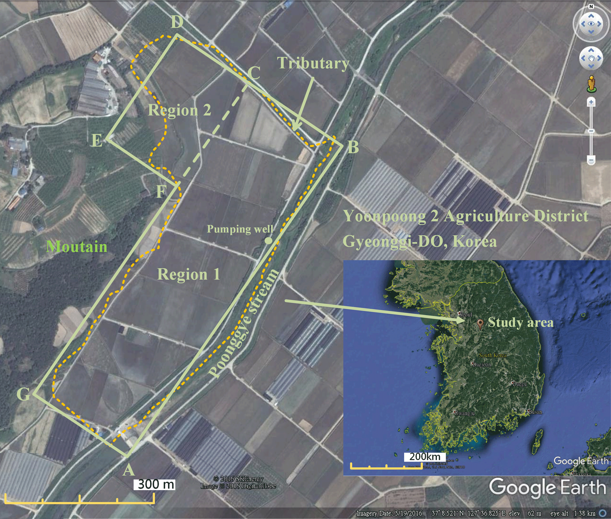
Figure 1Location of the fluvial aquifer. Note that this figure is modified from Google Earth.
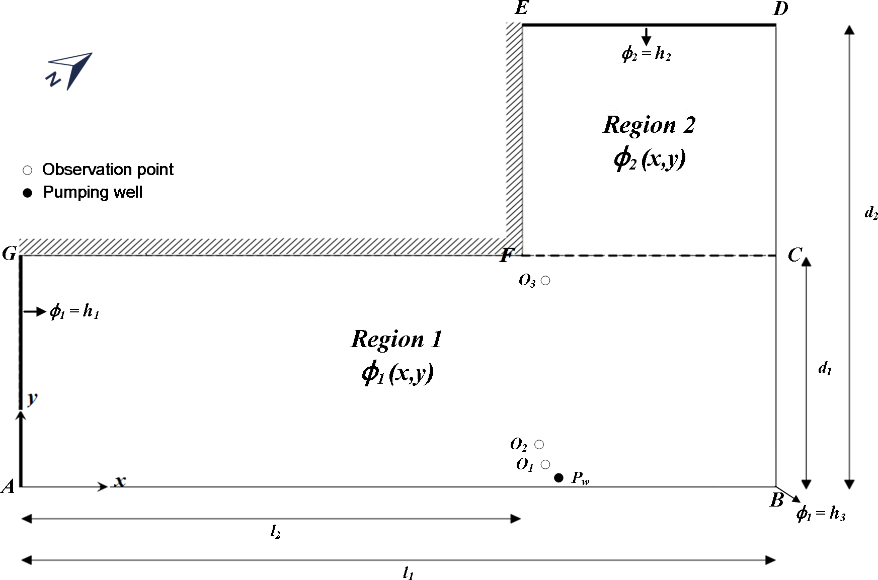
Figure 1 shows a fluvial plain located in the Yongpoong 2 Agriculture District, Gyeonggi-do, Korea whose characteristics are reported in Kihm et al. (2007). The west side of the plain is a mountainous area, where impermeable bedrock outcrops, and the Poonggye stream flows along the east side from the southwest corner toward the northeast corner. A tributary of Poonggye stream, entering the stream with nearly a right angle, is on the north side of the plain. The Poonggye stream and its tributary are perennial streams and almost fully penetrate the fluvial aquifer system (Kihm et al., 2007). The width of Poonggye stream is about 15 m as reported in River Information Management GIS (RIMGIS, 2013).
2.1 Conceptual model
The aquifer in the district is formed by fluvial deposits with a total thickness of 6 m and consists of a clay loam aquitard with a thickness of about 2.5 m underlain by a loamy sand layer with a thickness of about 3.5 m (Kihm et al., 2007). In order to develop an analytical model for solving the groundwater flow, the domain of the aquifer in this study is approximated to be L-shaped, as delineated in Fig. 2. Notice that in Fig. 1 the solid line denotes the outer boundary of the L-shaped aquifer in this study while the dashed line represents the simulation area in the work of Kihm et al. (2007). The origin of the coordinates in Fig. 2 is at the lower left corner of point A, which is at the intersection of boundary AB (i.e., a part of Poonggye stream) and boundary AG. The boundaries of the aquifer domain along EF and FG are impermeable bedrocks and thus regarded as impermeable boundaries. The annual average heads above the bottom of the aquifer are respectively identified as 5.18, 4.06, and 5.29 m at points A, B, and D (Kihm et al., 2007). The hydraulic heads along AG and DE are assumed equal to their average head values done by Kihm et al. (2007). In other words, the boundaries along AG and DE are assumed under the constant-head condition in our mathematical model. Physically, they do not coincide with streams and therefore do not contribute to SDR as calculated in Sect. 2.5 (“Stream depletion rate”). The boundaries AB and BD are designated to represent the Poonggye stream and its tributary, respectively. Kihm et al. (2007) fixed the hydraulic heads of Poonggye stream and its tributary at annual average water stages in their numerical simulations. Thus, this study considers that the stream has a perfect hydraulic connection with the aquifer and the stream stage varies linearly with distance. The average stream flow rate of the Poonggye stream with its tributary is about 100 m3 s−1 as reported by RIMGIS (2013, p. 90). Pumping wells in the conceptual model are assumed to fully penetrate the aquifer near the perennial stream AB as mentioned in Kihm et al. (2007), and therefore the hydraulic gradient in vertical direction is neglected. Todd and Mays (2005, p. 232) noticed that the discharge rates in a shallow well may range up to 500 m3 day−1 (0.01 m3 s−1) and the suction lifts should be less than 7 m for efficient and continuous service. Hence, the effect of pumping in a shallow well on the water table of the nearby stream is generally negligible. The annual average depth from the ground surface to the water table is 1.26 m with a spatial variation from 0.57 to 1.95 m in accordance with the average water stages in the streams AB and BD (Kihm et al., 2007). The depth for the aquifer system before pumping was estimated under the hydrostatic equilibrium condition and considering the effect of net annual average rainfall.
2.2 Mathematical model
As shown in Fig. 2, the aquifer is divided into two subregions named regions 1 and 2, and variables and are their corresponding hydraulic heads. Groundwater has been pumped by a total of M pumping wells in region 1 and N pumping wells in region 2, and all the pumping wells fully penetrate the aquifer. The coordinates of the kth well in region 1 and the lth well in region 2 are denoted as (x1k,y1k) and (x2l,y2l), respectively, and the pumping rate per unit thickness at the kth well is represented by Q1k [L2 T−1] and that at the lth well is Q2l [L2 T−1]. The governing equations describing 2-D hydraulic head distributions in region 1 and region 2 are respectively expressed as
where Kx [L T−1] and Ky [L T−1] are respectively the hydraulic conductivities in the x and y direction, and Ss [L−1] is the specific storage. The symbol δ represents the one-dimensional Dirac delta function [T−1]. The boundary conditions for region 1 are expressed as
Similarly, the boundary conditions for flow in region 2 are
The continuity requirements of the hydraulic head and flux along the interface CF are respectively
and
In order to express the solution in dimensionless form, the following dimensionless variables or parameters are introduced:
-
,
-
,
-
,
-
,
-
,
-
,
-
,
-
,
-
,
-
, and
-
,
where and stand for the dimensionless hydraulic heads in regions 1 and 2, respectively; t* refers to the dimensionless time during the test; κ1 and κ2 represent the anisotropic ratio of hydraulic conductivity in regions 1 and 2, respectively; x* and y*denote the dimensionless coordinates.
2.3 Steady-state solution for hydraulic head distribution
In order to compare the steady-state simulations of Kihm et al. (2007) without pumping, the steady-state solution for the hydraulic head distribution in the L-shaped aquifer is developed. Detailed derivation for the analytical solutions in steady state for regions 1 and 2 is given in Appendix A, and the results are expressed respectively as (Chu et al., 2012)
and
with
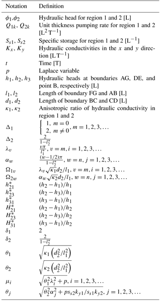
where the symbols and dimensionless variables Δ1, Δ2, λm, αn, Ω1m, Ω2n, , , , and are defined in Table 1. The coefficients C1m and D2n can be determined simultaneously by the continuity conditions of the hydraulic head and flux along the interface CF. The results are denoted as follows:
and
with
2.4 Transient solution for hydraulic head distribution
The semi-analytical solution of the model for transient hydraulic head distribution with the previous steady-state solution as the initial condition is developed via the methods of finite sine transform, finite cosine transform, and Laplace transform. The detailed derivation for the transient solution is given in Appendix B and the results of the dimensionless hydraulic heads in Laplace domain for regions 1 and 2 are respectively
and
with
where p is the Laplace variable and the symbols or dimensionless parameters δ1, δ2, αj, λi, μi, θ1, θ2, θj, Ω1i, Ω2j, and are introduced in Table 1.
The coefficients in Eqs. (26) and (27) are obtained via continuity requirements for the hydraulic head and flow flux at the interface CF. They can be solved simultaneously based on the following two equations
and
with
The coefficient can be determined by substituting Eq. (36) into Eq. (37); can then be obtained once is known. The hydraulic head distributions in the real time domain can be obtained by applying a numerical Laplace inversion scheme called the Stehfest algorithm (Stehfest, 1970), to Eqs. (26) and (27).
2.5 Stream depletion rate
Pumping in an aquifer near a stream often produces water filtration from the stream toward the well (Yeh et al., 2008). Water extracted by the pumping well comes from sources such as aquifer storage and nearby streams. The extraction rate from the stream is referred to as the stream depletion rate. Since the boundaries AG and ED do not correspond to streams in the physical world and are mathematically treated as constant head because they are far from the pumping well, only the water filtration from streams AB and BD to the nearby pumping well needs to be considered. The dimensionless solutions of SDR in the Laplace domain from the stream reaches AB and BD, denoted respectively as and , can be estimated by taking the derivatives of Eqs. (26) and (27) with respect to y and x, respectively, and then integrating along the reaches as
and
Further, the SDR solution for streams AB and BD in the real time domain are respectively denoted as SDRAB and SDRBD and also obtained by the Stehfest algorithm (Stehfest, 1970). The total dimensionless stream depletion rate (SDRT) in the time domain comes from the streams (AB and BD) and is expressed as
Since the depletion rate from constant-head boundaries AG and DE, which are far from the pumping well, can be neglected, the dimensionless storage release rate (SRR) representing the storage release rate due to compression of the aquifer matrix and expansion of groundwater in the pore space can be approximated as
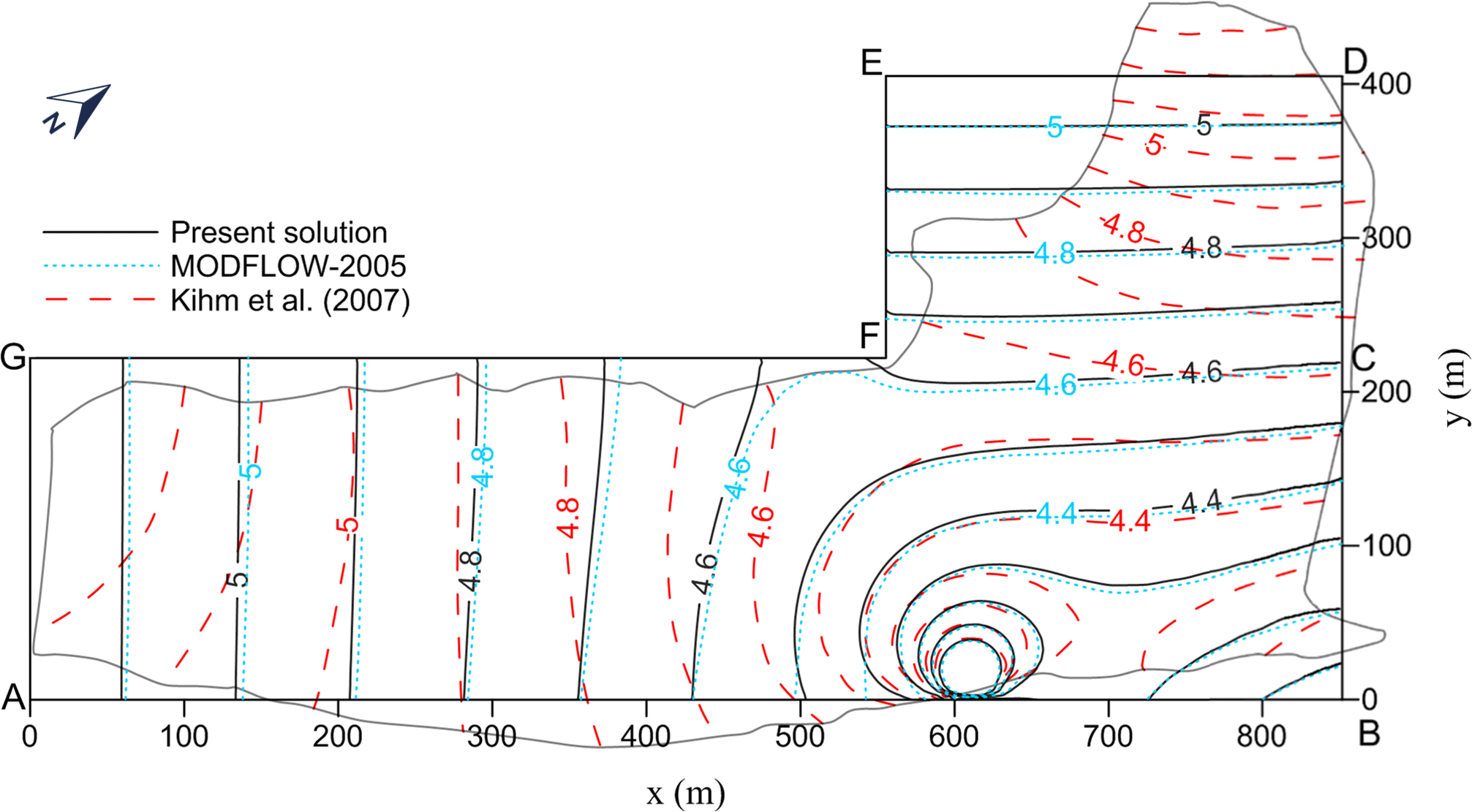
Figure 3Contours of the hydraulic head in the L-shaped aquifer predicted by the present solution, MODFLOW, and FEM simulations with an irregular outer boundary reported in Kihm et al. (2007).
3.1 Comparisons of the present solution with the MODFLOW solution
The software MODFLOW (USGS, 2005) is used to simulate the groundwater flow due to pumping in the L-shaped aquifer in the Yongpoong 2 Agriculture District with different hydraulic conductivities for the two layers. As shown in Fig. 1, region 1 has an area of 852 m × 222 m (i.e., l1×d1), while the area of region 2 is 297 m × 183 m (i.e., . Thus, the total area of these two regions is 243 495 m2, which is close to the area of the fluvial aquifer (246 500 m2) reported in Kihm et al. (2007). In the simulation of MODFLOW, the plane of the L-shaped aquifer is discretized with a uniform cell size of 3 m × 3 m. The aquifer thickness is 6 m and divided into two layers. The upper loam layer is 2.5 m thick and the lower sand layer is 3.5 m thick (Kihm et al. 2007). Within the aquifer domain, there is a total of 54 110 cells while the total number of cells are 42 032 and 12 078 respectively for region 1 and region 2. The boundary conditions specified for the L-shaped aquifer are the same as those defined in the mathematical model. The hydraulic heads along AG and DE are respectively h1=5.18 m and h2=5.29 m and the head at point B is h3=4.06 m. Following Kihm et al. (2007), the fluvial aquifer is considered isotropic and homogeneous in the horizontal direction. In other words, the hydraulic conductivities in the x and y directions are identical in both regions 1 and 2 (i.e., . However, the aquifer is heterogeneous in the vertical direction. It has two layers with hydraulic conductivity m s−1 for the upper layer and m s−1 for the lower layer. The specific storage of the aquifer in both regions 1 and 2 is 10−4 m−1 (Kihm et al., 2007). Consider that the pumping well Pw is located at (609 m, 9 m) in region 1 shown in Fig. 2 with a rate of 120 m3 day−1 for 1-year pumping. Figure 3 shows the hydraulic head distribution obtained from MODFLOW simulations and denoted as the dotted line.
The global behavior of a multilayered aquifer may be approximated with that of an equivalent homogeneous medium, whose hydraulic conductivity in the horizontal plane Kh may be evaluated as (Charbeneau, 2000):
where Ki is the hydraulic conductivity in the horizontal direction for layer i, bi is the thickness of layer i, and m is the number of the layers. Accordingly, the equivalent horizontal hydraulic conductivity Kh for the two-layered L-shaped aquifer is estimated as 1.2 × 10⁻⁴ m s−1. The solid line in Fig. 3 represents the hydraulic head distribution predicted by the present solution of Eqs. (26) and (27). The head distribution predicted by the present solution agrees with that of MODFLOW simulations except in the region near the no-flow boundary FG, where it has the largest relative deviation at 2.1 %. The comparison of the head distributions indicates that the use of equivalent hydraulic conductivity in the present model is appropriate and gives fairly good predicted results.
3.2 Steady-state head distribution without pumping in the Yongpoong 2 Agriculture District and impact of aquifer anisotropy
Kihm et al. (2007) reported the steady-state hydraulic head distribution, shown in Fig. 4 by the dashed line, for the FEM simulation without groundwater pumping in the two-layered irregular aquifer. Figure 4 also shows the steady-state head distributions predicted by the present solution of Eqs. (11) and (12) denoted as the solid line and by the MODFLOW denoted as the dotted line both for the L-shaped aquifer with m s−1 (i.e., evaluated based on Eq. (50) and other aquifer properties mentioned in Sect. 3.1. Similar to the pumping case, the predicted head distribution of the present solution conforms to the results of the MODFLOW simulation except in the area near the no-flow boundary FG. The result of the present solution shows that the predicted contour lines of the head distribution are nearly parallel to the boundary AG and perpendicular to the boundary FG in the region x≤200 m. Moreover, the predicted heads within the regions between 500 m 852 m and 0 m 200 m are reasonably close to the FEM results, which range from 4.3 to 4.7 m as shown in Fig. 4. The groundwater flows toward point B since it has the lowest water table within the problem domain.
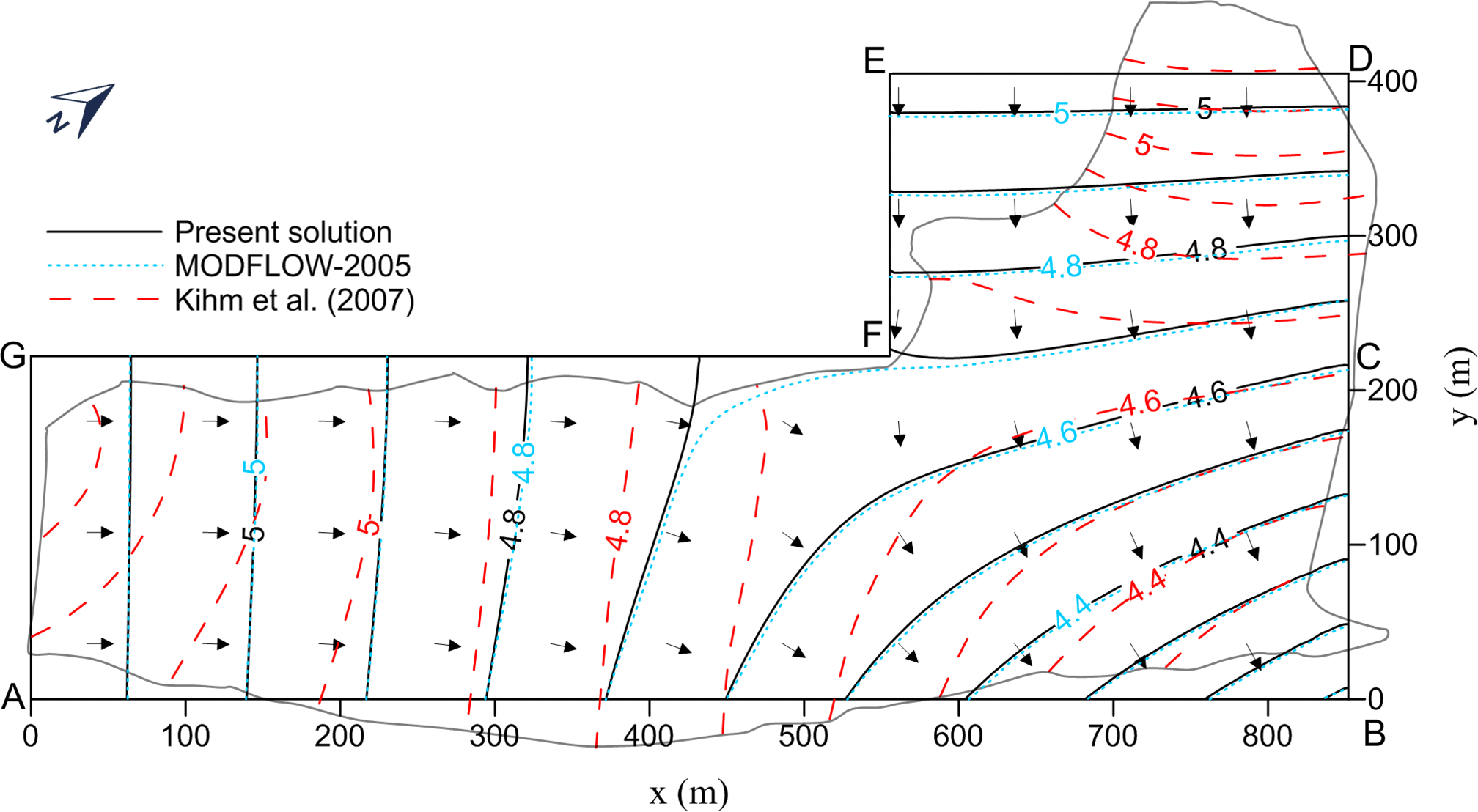
Figure 4Steady-state hydraulic head contours without pumping in the Yongpoong 2 Agriculture District.
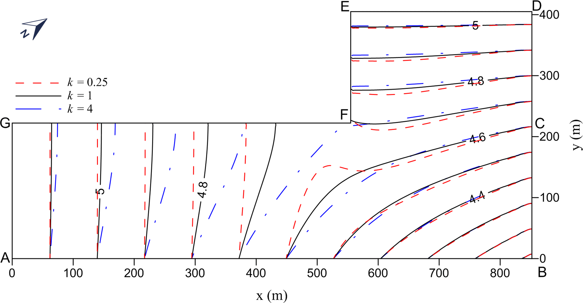
Figure 5Steady-state hydraulic head contours in the L-shaped aquifers with three different anisotropy ratios for .
Figure 5 shows the contour lines of the hydraulic head distribution for the isotropic case of by the solid line and for anisotropic cases of represented by the dashed–dotted line and by the dashed line. In these three cases, the head distributions are significantly different in the region where x≤600 m for the head ranging from 5 to 4.6 m. The largest head difference occurs near the upper boundary FG, reflecting the effects of no-flow condition and aquifer anisotropy on the flow pattern within this area.
3.3 Spatial head distributions due to pumping simulated by Kihm et al. (2007) and present solution after 1-year pumping
Figure 3 shows the spatial head distributions in the L-shaped aquifer predicted by the present solution and the MODFLOW for 1-year pumping at well Pw located at (609 m, 9 m) with a rate of 120 m3 day−1. In fact, Kihm et al. (2007) reported their FEM simulations for head distributions, groundwater-flow velocity, and land displacement for 1-year pumping at the well Pw with the same pumping rate mentioned above. They referred the simulated head results as initial steady-state distributions for the case of no pumping and final steady-state distributions for the case after 1-year pumping. The aquifer configuration in their FEM simulations and the simulated head distributions denoted as a dashed line are also demonstrated in Fig. 3. The figure indicates that the present solution gives good predicted head contours near the pumping well and a reasonably good result for the head distribution in region 1 as compared to those given by Kihm et al. (2007). The head distributions predicted by the FEM solution and present solution have obvious differences in the area far away from the pumping well. Those differences may be mainly caused by the difference in the physical domain considered in the FEM solution and the simplified domain used in the present solution. In addition, the mathematical model in Kihm et al. (2007) considered the unsaturated flow and deformation of the unsaturated soil, which may also affect the head distribution after pumping. Notice that the pumping well is very close to the stream boundary AB, which is the main stream in that area and provides a large amount of filtration water to the well. Hence, both groundwater flows in region 1 for x≤300 m (near boundary AG) and in region 2 for y≥200 m (near boundaries DE and EF) are not noticeably influenced by the pumping because these two regions are far away from the pumping well.
Three piezometers, O1, O2, and O3, were respectively installed at (597 m, 25 m), (594 m, 48 m), and (597 m, 204 m) as mentioned in Kihm et al. (2007) and indicated in Fig. 2. Note that O1 was installed near the stream AB while O3 was far away from the stream but close to the impermeable boundary FG. Figure 6 shows the temporal distributions of the hydraulic head measured at these three piezometers (i.e., HiO, and predicted by the FEM simulations (Kihm et al., 2007) (i.e., HiF), present solution (i.e., HiA), and MODFLOW simulations (i.e., HiM). This figure indicates that the hydraulic heads predicted by the present solution has a good agreement with those simulated by Kihm et al. (2007). The largest relative differences between the temporal hydraulic head predicted by the FEM and present solution are 0.58, 0.31, and 0.51 % m for O1, O2, and O3, respectively. As shown in Figs. 2 and 3, more than half of the aquifer boundary is surrounded by perennial streams and constant-head boundaries, and the pumping well is installed close to the main stream AB for stream filtration and screened in the highly permeable sand layer (Kihm et al., 2007). It is expected that the extracted water from the pumping well mainly comes from the stream AB, and the differences of the hydraulic heads from the observations (O1, O2, and O3) between the present solution and FEM simulation are insignificant because the boundary geometry near these observation in both the present solution and Kihm et al. (2007) are similar. These difference may be caused by the solid skeleton deformation and unsaturated flow considered in the FEM simulation of Kihm et al. (2007). Young's modulus (E) of the sand layer is 1.9×10⁷ N m−2 (Kihm et al., 2007), implying that the deformation of the sand layer due to pumping may be small. This is also seen in the vertical displacements reported in Kihm et al. (2007). The largest vertical displacement reported in Kihm et al. (2007) is only −0.003 m. Hence, the effect of land displacement during pumping may not significantly influence the hydraulic heads in piezometers. In addition, the unsaturated flow may slightly affect the saturated flow system. This is because the average thickness of the unsaturated zone is about 1.26 m, and it consists of a low permeability material (i.e., loam), which is 2 orders of magnitude less than that of the saturated zone (i.e., most of sand). As mentioned earlier, the pumping well is screened in the sand layer and the stream AB is the major source of extracted water. Therefore, the influence of the unsaturated zone on the saturated flow may be small. Under such hydrogeological conditions, the present solution yields a similar prediction for the temporal hydraulic head distribution as compared with those of FEM. Compared with the field observation, the differences of the predicted hydraulic head among FEM, the present solution, and MODFLOW are all less than 0.08 m at these three piezometers during 0.1 to 10 days. In addition, the largest relative differences between measured heads and predicted heads by the present solution at O1 to O3 during 0.1 to 5 days are respectively 1.64, 1.74, and 0.62 %, indicating that the present solution gives good predictions in the early pumping period. Moreover, the effects of unsaturated flow and land deformation on the groundwater flow in the Yongpoong aquifer are small and may be neglected. The hydraulic head at O1 drops more than those at O2 and O3, whereas the former is located closer to the pumping well Pw. Because Pw is very near the stream, the extracted water will be quickly contributed from the stream and therefore the drawdown at O1 will be soon stabilized. Figure 6 indicates that the hydraulic heads at O1−O3 predicted by the present solution reach steady state after t=100, 220, and 290 days, respectively.
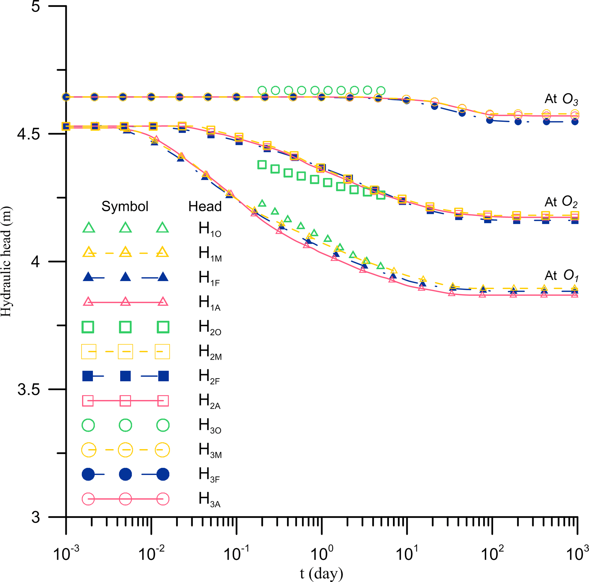
Figure 6Temporal distributions of the hydraulic head observed at piezometer Oi, HiO, and HiF are, respectively, the observations and FEM simulations reported in Kihm et al. (2007); HiA and HiM are the prediction of the present solution and MODFLOW, respectively, for i= 1, 2, 3.
3.4 Stream filtration in fluvial aquifer systems
Stream filtration can be considered as a problem associated with the interaction between the groundwater and surface water. The pumped water originated from the nearby stream is commonly supplied for irrigation, municipalities, and rural homes. In stream basins with several tributaries, pumping wells are often installed adjacent to the confluence of two tributaries in fluvial aquifers (Lambs, 2004).

Figure 7Temporal distributions of SDRs, SRR, and CHRs (constant head contribution rates) due to pumping at Pw.
It is of practical interest to know the temporal SDR distributions from both streams in the Yongpoong area when subject to pumping at Pw under a rate of 120 m3 day−1. The distances from Pw to the streams AB and BD are respectively 9 and 243 m. Figure 7 shows the temporal SDR distribution from each stream, indicating that SDRAB (i.e., SDR from stream AB) is significantly larger than SDRBD (SDR from stream BD) all the time. The steady-state values for SDRAB and SDRBD are respectively 0.81 and 0.19 when t≥220 days. This is due to the fact that the pumping well is closer to stream AB than stream BD and therefore water contributing to the pumping well from stream AB is much more than that from stream BD. Figure 7 also shows that the SDRT is zero and the aquifer storage release rate SRR is unity when t≤0.01 days, indicating that the well discharges totally from the aquifer storage in the early pumping period. Once the drawdown cone reaches the stream, the SDRT increases quickly with time while the SRR decreases continuously over the entire pumping period. It is interesting to mention that SDRT starts to contribute more water to the pumping than SRR when t≥5 days. Finally, the SDRT reaches unity and the SRR equals zero after t≥220 days, indicating that the aquifer system approaches steady state and all the extraction water comes from the streams.
A new semi-analytical model has been developed to analyze the 2-D hydraulic head distributions with and without pumping in a heterogeneous and anisotropic aquifer for an L-shaped domain bounded by two streams with linearly varying hydraulic heads. The method of domain decomposition is used to divide the aquifer into two regions for the development of the semi-analytical solution. The steady-state solution is first derived and used as the initial condition for the L-shaped aquifer system before pumping. The Laplace-domain solution of the model for transient head distribution in the aquifer subject to pumping is developed using the Fourier finite sine and cosine transform and the Laplace transform. The solution for SDR describing the filtration rate from two streams in an L-shaped aquifer is developed based on the head solution and Darcy's law. The Stehfest algorithm is then adopted to evaluate the time-domain results for both the head and SDR solutions in Laplace domain.
The 3-D finite difference model MODFLOW is first used to support the evaluation of the hydraulic head predictions by the present solution for the L-shaped two-layered aquifer system. The hydraulic head distributions predicted by present solutions agree fairly well over the entire aquifer except for the heads nearing the no-flow boundary. The solution for hydraulic head distribution in the L-shaped aquifer without pumping has been used to investigate the effect of anisotropic ratio (Kx∕Ky) on the steady-state flow system. It is interesting to note that the flow pattern in terms of lines of equal hydraulic head is strongly influenced by the value of anisotropic ratio for the region near the turning point of the L-shaped aquifer.
The transient solution for head distribution is employed to simulate the head distribution induced by pumping in the aquifer within the agriculture area of Gyeonggi-do, Korea. The aquifer is approximated as L-shaped in this study. The present solution delivers fairly good results in predicting the temporal hydraulic head distribution while comparing with those of FEM reported in previous study. Those simulation results seem to indicate that the effects of unsaturated flow and land displacement on the groundwater flow are not significant and may be ignorable. The largest relative differences between the measured heads and the predicted heads by the present solution at three piezometers are less than 1.74 %.
The SDR solution is first used to evaluate the steady-state SDR from each of the nearby streams for the Yongpoong aquifer subject to a specific pumping rate. The solution is also employed to determine the temporal contribution rates from the aquifer storage and the streams toward the extraction well.
All the required parameters are provided in the study. The data sets of observations and FEM model were collected from that reported in Kihm et al. (2007). In addition, the data sets of present solution and MODFLOW are freely available upon request by contacting the first or corresponding author.
On the basis of dimensionless variables and parameters defined in Sect. 2.2, Eqs. (1) and (2) can be written respectively as
and
The dimensionless boundary conditions for region 1 can be expressed as
and for region 2 as
The continuity requirements of the hydraulic head and flux at the region interface in dimensionless form are respectively expressed as
and
The steady-state solution for groundwater flow in an L-shaped aquifer without pumping can be solved after removing the source/sink term in Eqs. (A1) and (A2). Multiplying Eq. (A1) by sin (λmx*) and integrating it for x* from 0 to 1 in region 1 with boundary conditions Eqs. (A3) and (A4), Eq. (A1) is then transformed to
with
where , λm=mπ and .
Similarly, Eq. (A2) can be transformed via multiplying Eq. (A2) by and integrating it for x* from to 1 in region 2 with boundary conditions Eqs. (A7) and (A8). The result is
with
where , and .
The general solutions of Eqs. (A12) and (A14) can be written respectively as
and
The coefficients C1m and C2m in Eq. (A16) are determined by Eq. (A5) and the result is
Similarly, the coefficients D1n and D2n in Eq. (A17) are determined based on Eq. (A10) as
Substituting Eq. (A18) into Eq. (A16), the inversion of leads to Eq. (12) for the dimensionless hydraulic head distribution in region 1. Similarly, the inversion of for region 2 after substituting Eq. (A19) into Eq. (A17) results in Eq. (13). Based on Eqs. (A10) and (A11), the coefficients of C1m and D2n can be simultaneously determined and the results are respectively given in Eqs. (18) and (19).
Multiplying Eq. (A1) by sin (λix*) and integrating it for x* from 0 to 1 in region 1 with Eqs. (A3) and (A4), Eq. (A1) can be transformed as
with
where , , and λi=iπ, .
Similarly, Eq. (A2) can be transformed via multiplying Eq. (A2) by cos (αjx*) and integrating it for x* from to 1 in region 2 with Eqs. (A7) and (A8). The result is
with
where , and for . Then, taking Laplace transforms to Eq. (B1) results in
where is the steady-state solution of region 1. Hence, Eq. (B5) can be organized as
where , with the Laplace transform of defined as
Similarly, the Laplace transform of Eq. (B3) is obtained as
where is the steady-state solution of region 2. Thus, Eq. (B8) can be written as
where , with the Laplace transform of defined as
The general solution of Eq. (B6) can be expressed as
where the particular solution is
with
Moreover, Eq. (B9) can also be expressed as
in which is
with
On the basis of Eq. (A5), the coefficient T2i in Eq. (B11) can be determined in terms of T1i as
The solution for hydraulic head distribution in region 1 is given as Eq. (26), which is obtained by substituting Eq. (B17) into Eq. (B11) and then taking the following inverse Fourier transform to Eq. (B11) denoted as
with
Similarly, T1j in Eq. (B14) can be obtained based on Eq. (A9) as
The solution for region 2 is Eq. (27), which is acquired by substituting Eq. (B20) into Eq. (B14) and then taking the following inverse Fourier transform to Eq. (B14) expressed as
with
Furthermore, the coefficients of and can be simultaneously determined by Eqs. (A10) and (A11). The results are respectively given in Eqs. (36) and (37).
The authors declare that they have no conflict of interest.
This study was partly supported by the grants from Taiwan Ministry of Science
and Technology under the contract numbers MOST 105-2221-E-009-043-MY2 and
MOST 106-2221-E-009 -066. The authors would like to thank the editor, two
anonymous reviewers, and David Ferris for their valuable and constructive
comments that greatly improved the manuscript.
Edited by: Mauro Giudici
Reviewed by: two anonymous referees
Asadi-Aghbolaghi, M. and Seyyedian, H.: An analytical solution for groundwater flow to a vertical well in a triangle-shaped aquifer, J. Hydrol., 393, 341–348, https://doi.org/10.1016/j.jhydrol.2010.08.034, 2010.
Chan, Y. K., Mullineux, N., and Reed, J. R.: Analytic solutions for drawdowns in rectangular artesian aquifers, J. Hydrol., 31, 151–160, https://doi.org/10.1016/0022-1694(76)90026-3, 1976.
Chan, Y. K., Mullineux, N., and Reed, J. R.: Analytic solution for drawdown in an unconfined-confined rectangular aquifer, J. Hydrol., 34, 287–296, https://doi.org/10.1016/0022-1694(77)90136-6, 1977.
Chan, Y. K., Mullineux, N., Reed, J. R., and Wells, G. G.: Analytic solutions for drawdowns in wedge-shaped artesian aquifers, J. Hydrol., 36, 233–246, https://doi.org/10.1016/0022-1694(78)90146-4, 1978.
Charbeneau, R. J.: Groundwater Hydraulics and Pollutant Transport, Prentice Hall, Upper Saddle River, NJ, 2000.
Chen, Y. J., Yeh, H. D., and Yang, S. Y.: Analytical Solutions for Constant-Flux and Constant-Head Tests at a Finite-Diameter Well in a Wedge-Shaped Aquifer, J. Hydraul. Eng., 135, 333–337, 10.1061/(ASCE)0733-9429(2009)135:4(333), 2009.
Chu, Y. J., Lin, C. C., and Yeh, H. D.: Steady-state groundwater flow in an anisotropic aquifer with irregular boundaries, International Conference on Sustainable Environmental Technologies, Bangkok, Thailand, 2012.
Corapcioglu, M. Y., Borekci, O., and Haridas, A.: Analytical solutions for rectangular aquifers with third-kind (Cauchy) boundary conditions, Water Resour. Res., 19, 523–528, https://doi.org/10.1029/WR019i002p00523, 1983.
Daly, C. J. and Morel-Seytoux, H. J.: An integral transform method for the linearized Boussinesq Groundwater Flow Equation, Water Resour. Res., 17, 875–884, https://doi.org/10.1029/WR017i004p00875, 1981.
Falade, G. K.: On the flow of fluid in the wedged anisotropic porous domain, J. Hydrol., 58, 111–121, https://doi.org/10.1016/0022-1694(82)90072-5, 1982.
Holzbecher, E.: Analytical solution for two-dimensional groundwater flow in presence of two isopotential lines, Water Resour. Res., 41, W12502, https://doi.org/10.1029/2005WR004583, 2005.
Huang, C.-S., Chen, J.-J., and Yeh, H.-D.: Approximate analysis of three-dimensional groundwater flow toward a radial collector well in a finite-extent unconfined aquifer, Hydrol. Earth Syst. Sci., 20, 55–71, https://doi.org/10.5194/hess-20-55-2016, 2016.
Jafari, F., Javadi, S., Golmohammadi, G., Karimi, N., and Mohammadi, K.: Numerical simulation of groundwater flow and aquifer-system compaction using simulation and InSAR technique: Saveh basin, Iran, Environ. Earth Sci., 75, 833, https://doi.org/10.1007/s12665-016-5654-x, 2016.
Kantorovich, L. V. and Krylov, V. I.: Approximate Methods of Higher Analysis, Interscience, New York, 1958.
Kacimov, A. R., Kayumov, I. R., and Al-Maktoumi, A.: Rainfall induced groundwater mound in wedge-shaped promontories: The Strack–Chernyshov model revisited. Adv. Water Resour., 97, 110–119, https://doi.org/10.1016/j.advwatres.2016.08.011, 2016.
Kacimov, A. R., Maklakov, D. V., Kayumov, I. R., and Al-Futaisi, A.: Free Surface flow in a microfluidic corner and in an unconfined aquifer with accretion: The Signorini and Saint-Venant analytical techniques revisited, Transport in Porous Med., 116, 115–142, https://doi.org/10.1007/s11242-016-0767-y, 2017.
Kihm, J.-H., Kim, J.-M., Song, S.-H., and Lee, G.-S.: Three-dimensional numerical simulation of fully coupled groundwater flow and land deformation due to groundwater pumping in an unsaturated fluvial aquifer system, J. Hydrol., 335, 1–14, https://doi.org/10.1016/j.jhydrol.2006.09.031, 2007.
Kuo, M. C. T., Wang, W. L., Lin, D. S., Lin, C. C., and Chiang, C. J.: An Image-Well Method for Predicting Drawdown Distribution in Aquifers with Irregularly Shaped Boundaries, Ground Water, 32, 794–804, https://doi.org/10.1111/j.1745-6584.1994.tb00921.x, 1994.
Lambs, L.: Interactions between groundwater and surface water at river banks and the confluence of rivers, J. Hydrol., 288, 312–326, https://doi.org/10.1016/j.jhydrol.2003.10.013, 2004.
Latinopoulos, P.: Well recharge in idealized rectangular aquifers, Adv. Water Resour., 5, 233–235, https://doi.org/10.1016/0309-1708(82)90006-9, 1982.
Latinopoulos, P.: Periodic recharge to finite aquifiers from rectangular areas, Adv. Water Resour., 7, 137–140, https://doi.org/10.1016/0309-1708(84)90043-5, 1984.
Latinopoulos, P.: Analytical solutions for periodic well recharge in rectangular aquifers with third-kind boundary conditions, J. Hydrol., 77, 293–306, https://doi.org/10.1016/0022-1694(85)90213-6, 1985.
Li, P., Stagnitti, F., and Das, U.: A new analytical solution for Laplacian porous-media flow with arbitrary boundary shapes and conditions, Math. Comput. Model., 24, 3–19, https://doi.org/10.1016/S0895-7177(96)00160-4, 1996.
Li, H. and Jiao, J. J.: Tidal groundwater level fluctuations in L-shaped leaky coastal aquifer system, J. Hydrol., 268, 234–243, https://doi.org/10.1016/S0022-1694(02)00177-4, 2002.
Loudyi, D., Falconer, R. A., and Lin, B.: Mathematical development and verification of a non-orthogonal finite volume model for groundwater flow applications, Adv. Water Resour., 30, 29–42, https://doi.org/10.1016/j.advwatres.2006.02.010, 2007.
Lu, C., Xin, P., Li, L., and Luo, J.: Steady state analytical solutions for pumping in a fully bounded rectangular aquifer, Water Resour. Res., 51, 8294–8302, https://doi.org/10.1002/2015WR017019, 2015.
Mackowski, D. W.: Conduction Heat Transfer: Notes for MECH 7210, Mechanical Engineering Department, Auburn University, 2011.
Mahdavi, A. and Seyyedian, H.: Steady-state groundwater recharge in trapezoidal-shaped aquifers: A semi-analytical approach based on variational calculus, J. Hydrol., 512, 457–462, https://doi.org/10.1016/j.jhydrol.2014.03.014, 2014.
Matthews, C. S., Brons, F., and Hazebroek, P.: A method for determination of average pressure in bounded reservoir, T. AIME, 201, 182–191, 1954.
Mohanty, S., Jha, M. K., Kumar, A., and Panda, D. K.: Comparative evaluation of numerical model and artificial neural network for simulating groundwater flow in Kathajodi–Surua Inter-basin of Odisha, India, J. Hydrol., 495, 38–51, https://doi.org/10.1016/j.jhydrol.2013.04.041, 2013.
Patel, A. and Serrano, S. E.: Decomposition solution of multidimensional groundwater equations, J. Hydrol., 397, 202–209, https://doi.org/10.1016/j.jhydrol.2010.11.032, 2011.
Read, W. W. and Volker, R. E.: Series solutions for steady seepage through hillsides with arbitrary flow boundaries, Water Resour. Res., 29, 2871–2880, https://doi.org/10.1029/93WR00905, 1993.
River Information Management GIS (RIMGIS): Korean river list and related data, available at: http://mobile.river.go.kr/Mobiles/sub_03/Books/\% ED\% 95\% 9C\% EA\% B5\% AD\% ED\% 95\% 98\% EC\% B2\% 9C\% EC\% 9D\% BC\% EB\% 9E\% 8C(2012.12.31\% EA\% B8\% B0\% EC\% A4\% 80).pdf (last access: 4 September 2017), 2013 (in Korean).
Samani, N. and Zarei-Doudeji, S.: Capture zone of a multi-well system in confined and unconfined wedge-shaped aquifers, Adv. Water Resour., 39, 71–84, https://doi.org/10.1016/j.advwatres.2012.01.004, 2012.
Samani, N. and Sedghi, M. M.: Semi-analytical solutions of groundwater flow in multi-zone (patchy) wedge-shaped aquifers, Adv. Water Resour., 77, 1–16, https://doi.org/10.1016/j.advwatres.2015.01.003, 2015.
Serrano, S. E.: A simple approach to groundwater modelling with decomposition, Hydrol. Sci. J., 58, 177–185, 10.1080/02626667.2012.745938, 2013.
Stehfest, H.: Algorithm 368: Numerical inversion of Laplace transforms, Commun. ACM, 13, 47–49, https://doi.org/10.1145/361953.361969, 1970.
Sun, H.: A two-dimensional analytical solution of groundwater response to tidal loading in an estuary, Water Resour. Res., 33, 1429–1435, https://doi.org/10.1029/97WR00482, 1997.
Taigbenu, A. E.: Green element simulations of multiaquifer flows with a time-dependent Green's function, J. Hydrol., 284, 131–150, https://doi.org/10.1016/j.jhydrol.2003.07.002, 2003.
Todd, D. K. and Mays, L. W.: Groundwater Hydrology, 3rd edn., Wiley, 2005.
US Geological Survey: MODFLOW-2005: The US geological survey modular groundwater model- the groundwater flow process, US Geological Survey Techniques and Methods, 6-A16, 2005
Younger, P. L.: Groundwater in the Environment: An Introduction, 1st edn., Wiley, 2007.
Yeh, H.-D., Chang, Y.-C., and Zlotnik, V. A.: Stream depletion rate and volume from groundwater pumping in wedge-shape aquifers, J. Hydrol., 349, 501–511, https://doi.org/10.1016/j.jhydrol.2007.11.025, 2008.
- Abstract
- Introduction
- Methodology
- Comparisons of the present solution, numerical solutions, and field-observed data
- Conclusions
- Code and data availability
- Appendix A: Steady-state solution for flow in an L-shaped aquifer without pumping
- Appendix B: Transient solutions for an L-shaped aquifer
- Competing interests
- Acknowledgements
- References