the Creative Commons Attribution 4.0 License.
the Creative Commons Attribution 4.0 License.
 | 18 Apr 2018
Regional evapotranspiration from an image-based implementation of the Surface Temperature Initiated Closure (STIC1.2) model and its validation across an aridity gradient in the conterminous US
Kaniska Mallick
Nathaniel A. Brunsell
Ge Sun
Meha Jain
Recent studies have highlighted the need for improved characterizations of aerodynamic conductance and temperature (gA and T0) in thermal remote-sensing-based surface energy balance (SEB) models to reduce uncertainties in regional-scale evapotranspiration (ET) mapping. By integrating radiometric surface temperature (TR) into the Penman–Monteith (PM) equation and finding analytical solutions of gA and T0, this need was recently addressed by the Surface Temperature Initiated Closure (STIC) model. However, previous implementations of STIC were confined to the ecosystem-scale using flux tower observations of infrared temperature. This study demonstrates the first regional-scale implementation of the most recent version of the STIC model (STIC1.2) that integrates the Moderate Resolution Imaging Spectroradiometer (MODIS) derived TR and ancillary land surface variables in conjunction with NLDAS (North American Land Data Assimilation System) atmospheric variables into a combined structure of the PM and Shuttleworth–Wallace (SW) framework for estimating ET at 1 km × 1 km spatial resolution. Evaluation of STIC1.2 at 13 core AmeriFlux sites covering a broad spectrum of climates and biomes across an aridity gradient in the conterminous US suggests that STIC1.2 can provide spatially explicit ET maps with reliable accuracies from dry to wet extremes. When observed ET from one wet, one dry, and one normal precipitation year from all sites were combined, STIC1.2 explained 66 % of the variability in observed 8-day cumulative ET with a root mean square error (RMSE) of 7.4 mm/8-day, mean absolute error (MAE) of 5 mm/8-day, and percent bias (PBIAS) of −4 %. These error statistics showed relatively better accuracies than a widely used but previous version of the SEB-based Surface Energy Balance System (SEBS) model, which utilized a simple NDVI-based parameterization of surface roughness (zOM), and the PM-based MOD16 ET. SEBS was found to overestimate (PBIAS = 28 %) and MOD16 was found to underestimate ET (PBIAS = −26 %). The performance of STIC1.2 was better in forest and grassland ecosystems as compared to cropland (20 % underestimation) and woody savanna (40 % overestimation). Model inter-comparison suggested that ET differences between the models are robustly correlated with gA and associated roughness length estimation uncertainties which are intrinsically connected to TR uncertainties, vapor pressure deficit (DA), and vegetation cover. A consistent performance of STIC1.2 in a broad range of hydrological and biome categories, as well as the capacity to capture spatio-temporal ET signatures across an aridity gradient, points to the potential for this simplified analytical model for near-real-time ET mapping from regional to continental scales.
- Article
(13121 KB) - Full-text XML
-
Supplement
(453 KB) - BibTeX
- EndNote


Evapotranspiration (ET) is highly variable in space and time and plays a fundamental role in hydrology and land–atmosphere interactions. Over the past few decades, the use of satellite data to map regional-scale ET has advanced considerably. This is due to the advancements in ET modeling as well as progress in thermal remote sensing satellite missions, and our ability to retrieve the land surface temperature (LST) or radiometric surface temperature (TR) that is highly sensitive to evaporative cooling and surface moisture variations. Because LST governs the land surface energy budget (Kustas and Norman, 1996; Kustas and Anderson, 2009), thermal ET models principally focus on the surface energy balance (SEB) approach in which TR represents the lower boundary condition to constrain energy–water fluxes (Anderson et al., 2012). Contemporary SEB models emphasize estimating aerodynamic conductance (gA) and sensible heat flux (H) while solving ET (i.e., latent heat flux, λE) as a residual SEB component. Despite many advancements in mapping spatially distributed ET, some fundamental challenges remain in existing SEB algorithms including (a) the inequality between TR and the aerodynamic temperature (T0), which is essentially responsible for the exchanges of H and λE (Chávez et al., 2010; Boulet et al., 2012); (b) a non-unique relationship between T0 and TR due to differences between the roughness lengths (i.e., effective source/sink heights) for momentum (z0M) and heat (z0H) within vegetation canopy and substrate complex (Troufleau et al., 1997; Paul et al., 2014; van Dijk et al., 2015b); (c) the unavailability of a universally agreed model to estimate T0 (Colaizzi et al., 2004); and (d) the lack of a physically based or analytical gA model. To overcome these challenges, we implement the current version of a recently developed analytical ET model, the Surface Temperature Initiated Closure (STIC, version 1.2; Mallick et al., 2014, 2015, 2016), using the Moderate Resolution Imaging Spectroradiometer (MODIS) data to develop spatially distributed ET maps.
In state-of-the-art SEB models, an emphasis on estimating gA and H is laid due to the perception of the broad applicability of the Monin–Obukhov similarity theory (MOST) or Richardson number (Ri) criteria, and the requirement of minimum inputs for determining these variables. However, these approaches created additional uncertainties, particularly in accommodating T0 vs. TR inequalities, as well as adapting the differences between z0M and z0H (Paul et al., 2014). Compensating these temperature and roughness length disparities consequently led to the inception of the kB−1 term as a fitting parameter (Verhoef et al., 1997a), and later the progress of the two-source ET model (Kustas and Norman, 1997; Norman et al., 1995; Anderson et al., 2011). Although useful, the above approaches still rely on empirical response functions of roughness components to characterize gA that has an uncertain transferability in space and time (Holwerda et al., 2012; van Dijk et al., 2015b). In contemporary SEB modeling, gA sub-models are stand-alone and lack the necessary physical feedbacks between the conductances, T0, and vapor pressure deficit surrounding the evaporating surface (D0). The feedback of gA on gC and D0 is critical in semiarid and arid ecosystems (Kustas et al., 2016), where soil moisture stress and sparse vegetation can cause substantial disparities between TR and T0 (Kustas et al., 2016; Paul et al., 2014; Timmermans et al., 2013; Gokmen et al., 2012). Therefore, thermal-based ET modeling needs explicit consideration of these important biophysical feedbacks to overcome the existing gA and T0 uncertainties in regional-scale ET mapping (Kustas et al., 2016). Hence, a genuine question in regional ET mapping is the following: how can state-of-the-art SEB models overcome the existing challenges in regional evapotranspiration mapping that arise due to uncertain conductance parameterizations, and can analytical models help this verification process?
The STIC formulation provides analytical solutions to gA, T0, and canopy (or surface) conductance (gC), and simultaneously captures the critical feedbacks between gA,gC, T0, and vapor pressure deficit surrounding the evaporating surface (D0) thereby obtaining a “closure” of the SEB . The prime focus of STIC (Mallick et al., 2014, 2015, 2016) is based on physical integration of TR into the Penman–Monteith (PM) equation, which is fundamentally constrained to account for the necessary feedbacks between ET, TR, DA, gA, and gC (Monteith, 1965). Monteith (1981) highlighted the fact that the biophysical conductances (i.e., gA and gC) regulating ET are heavily temperature dependent, after which a stream of research demonstrated the dominant control of TR on gC and associated canopy-scale aerodynamics (Moffett and Gorelick, 2012; Blonquist et al., 2009). Somewhat surprisingly, the idea of integrating TR into the PM model was never attempted because of complexities associated with gC parameterization (Bell et al., 2015; Matheny et al., 2014), until the concept of STIC was formulated (Mallick et al., 2014, 2015). The recent version of STIC, STIC1.2, combines PM with the Shuttleworth–Wallace (SW) model (Shuttleworth and Wallace, 1985) to estimate the source/sink height temperature and vapor pressure (T0 and e0; Mallick et al., 2016). By algebraic reorganization of aerodynamic equations of H and λE, Bowen ratio evaporative fraction hypothesis (Bowen, 1926) and modified advection-aridity hypothesis (Brutsaert and Stricker, 1979), STIC1.2 formulates multiple state equations where the state equations were constrained with an aggregated moisture availability factor (M). Through physically linking M with TR and the source/sink height dew point temperature (TSD), STIC1.2 established a direct feedback between TR and ET, while simultaneously overcoming the empirical uncertainties in conductances and T0 estimations.
Despite providing analytical solutions for the key conductances in PM-based ET modeling, the STIC1.2 model has yet to gain a profound interest among the thermal remote sensing community and those interested in regional-scale ET modeling. This could largely be attributed to the fact that the model is only used for understanding ecosystem-scale ET partitioning and their biophysical controls at the eddy covariance (EC) footprints (Mallick et al., 2015, 2016), where all the necessary forcing variables were measured at the flux tower sites. In this paper, we present the first ever implementation of the STIC1.2 model using MODIS LST and associated land surface products, and its validation in 13 core AmeriFlux sites across an aridity gradient in the conterminous US in three different precipitation conditions representing dry, normal, and wet years. ET estimates from STIC1.2 are also compared against two parametric ET models, namely SEBS (Surface Energy Balance System; Su, 2002) and MOD16 (Mu et al., 2007, 2011). Through the implementation and validation of the STIC1.2 model at a regional-scale, the current study addresses the following research questions:
-
What is the performance of STIC1.2 when applied at the regional-scale across an aridity gradient and during contrasting rainfall years in the conterminous US?
-
How does STIC1.2-derived ET compare against other global ET models that are driven by TR and relative humidity (RH)?
-
Under which conditions do the models agree and which factors cause their differences?
-
How well do the models capture spatio-temporal ET variability across an aridity gradient?
A description of methods including models, study sites, dataset, and data processing is given in Sect. 2, followed by the results in Sect. 3. An extended discussion of the results and potential of the method in thermal remote sensing applications is elaborated in Sects. 4 and 5, respectively. Symbols used for variables in this study are listed in the Appendix in Table A1.
2.1 Model descriptions
Most SEB models consist of several modules for estimating net radiation (RN), ground heat flux (G), and partitioning of available energy (ϕ = RN − G) into H and λE through the derivation of evaporative fraction (Λ). Λ is defined as the ratio of λE to ϕ. In this paper, we used the widely used net radiation balance equation (Eq. 1) to compute RN (Allen et al., 2007, 2011) and the formulation of Bastiaanssen (2000) to compute G (Eq. 4) in SEBS and STIC1.2.
where RS is the incoming shortwave radiation, αo is the surface albedo, εo is the surface emissivity, NDVI is the normalized difference vegetation index, λ is the latent heat of vaporization, and Rld and Rlu are incoming and outgoing longwave radiation, respectively. Using the formulation of Allen et al. (2007) and Bastiaanssen (2000) for estimating RN and G, respectively, we found that the estimated 8-day mean RN and G during the Terra overpass time were within 14 % of the observed RN and G at the flux sites (Fig. S1 in the Supplement).
While the derivation of H in SEBS is based on an aerodynamic equation (Su, 2002), SEBS estimates λE as the residual of the SEB (i.e., λE = RN − G− H). On the contrary, STIC1.2 directly estimates H and λE through the PM equation (Mallick et al., 2016) by solving state equations for the conductances. MOD16 estimates λE directly using a modified PM framework (Mu et al., 2007, 2011), where the conductances are estimated based on a biome property lookup table (BPLUT) and meteorological scaling functions. As discussed in Sect. 1, there exist some fundamental differences among STIC1.2, SEBS, and MOD16. However, since the primary focus of the paper is the regional-scale implementation and evaluation of the STIC1.2 model, we only provide detailed descriptions of STIC1.2 and suggest readers follow associated literature for detailed descriptions of the other two models (see Sects. 2.1.2 and 2.1.3). The key model structures of SEBS and MOD16 are briefly explained in Sects. 2.1.2 and 2.1.3.
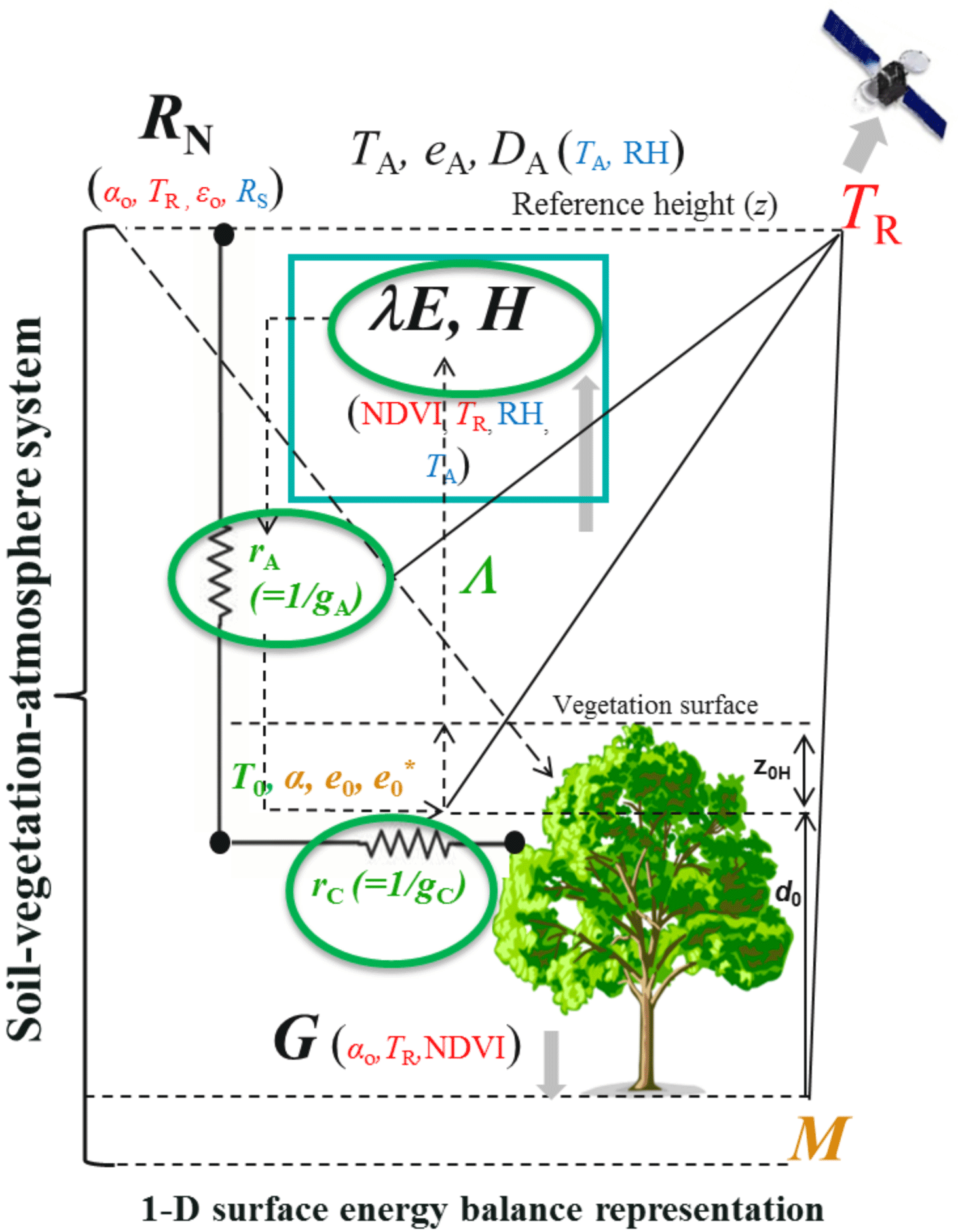
Figure 1Schematic representation of one-dimensional description of STIC1.2 showing how a feedback is established between the surface layer evaporative fluxes and source/sink height mixing and coupling (dotted arrows between e0, , gA and gC, and λE). Here rA and rC (gA and gC) are the aerodynamic and canopy resistances (conductances); is the saturation vapor pressure at the source/sink height; T0 is the source/sink height temperature (i.e., aerodynamic temperature) that is responsible for transferring the sensible heat (H); e0 and eS are the vapor pressure at the source/sink height and the surface, respectively; z0H is the roughness length for heat transfer, d0 is the displacement height; TR is the radiometric surface temperature; M is the surface moisture availability or evaporation coefficient; RN and G are net radiation and ground heat fluxes; TA, eA, and DA are temperature, vapor pressure, and vapor pressure deficit at the reference height (z); and λE and H are latent and sensible heat fluxes, respectively. Inputs from MODIS land surface products and gridded weather datasets for the regional implementation of STIC1.2 in this paper are shown in red and blue fonts, respectively. Text in green font represents the state variables for which an analytical solution was obtained by solving the “state equations” (Eqs. 7–10). Text in orange are the variables that were obtained iteratively along with the state variables.
2.1.1 STIC1.2
STIC1.2 is the most recent version of the original STIC formulation (Mallick et al., 2014, 2015), which is a one-dimensional physically based SEB model that treats the vegetation–substrate complex as a single unit (Fig. 1). The fundamental assumption in STIC1.2 is the first order dependency of gA and gC on T0 and soil moisture through TR. Such an assumption allows for a direct integration of TR in the PM equation (Mallick et al., 2016). The common expression for λE in the PM equation is
where ρA is the air density (kg m−3), cP is the specific heat of air (J kg−1 K−1), γ is the psychrometric constant (hPa K−1), s is the slope of the saturation vapor pressure vs. TA (hPa K−1), DA is the saturation deficit of the air (hPa) at the reference level, and ϕ is the net available energy (i.e., RN − G). The units for all the surface fluxes and conductances are W m−2 and m s−1, respectively.
In Eq. (5), the two biophysical conductances (gA and gC) are unknown and the STIC1.2 methodology is based on finding analytical solutions for the two unknown conductances to directly estimate ET (Mallick et al., 2014, 2015). The need for such analytical estimation of these conductances is motivated by the fact that gA and gC can neither be measured at the canopy nor larger spatial scales, and there is not an appropriate model of gA and gC that currently exists (Matheny et al., 2014; van Dijk et al., 2015b). By integrating TR with standard SEB theory and vegetation biophysical principles, STIC1.2 formulates multiple state equations (Eqs. 7–10 below) in order to eliminate the need for empirical parameterization for gA, gC, and T0. The state equations for the conductances and T0 were expressed as a function of those variables that can be estimated by remote sensing observations. In the state equations, a direct connection of TR is established by estimating an aggregated moisture availability index (M). The information of M is subsequently used in the state equations of gA, gC, T0, and evaporative fraction (Λ; Eqs. 7–10 below), which is eventually propagated into their analytical solutions. M is a unitless quantity, which describes the relative wetness of the surface and also controls the transition from potential to actual evaporation. Therefore, M is critical for providing a constraint against which the conductances can be estimated. Since TR is extremely sensitive to the surface water content variations, it is extensively used for estimating M in a physical retrieval scheme (details in Appendix A3, also in Mallick et al., 2016). We hypothesize that linking M with the biophysical conductances will simultaneously integrate the information of TR into the PM equation (Eq. 5) in the framework of STIC1.2.
In STIC1.2, the estimation of M is based on Venturini et al. (2008), where M is expressed as the ratio of the vapor pressure difference between the source/sink height and air to the vapor pressure deficit between source/sink height and the atmosphere as follows.
where e0 and are the actual and saturation vapor pressure at the source/sink height; eA is the atmospheric vapor pressure; is the saturation vapor pressure at the surface; TD is the air dew point temperature; s1 and s2 are the psychrometric slopes of the saturation vapor pressure and temperature between (TSD–TD) vs. (e0–eA) and (TR–TD) vs. (–eA) relationship (Venturini et al., 2008); and κ is the ratio between (–eA) and (–eA). Despite T0 driving the sensible heat flux, the comprehensive dry–wet signature of the underlying surface due to aggregated moisture variability is directly reflected in TR (Kustas and Anderson, 2009). Therefore, using TR in the denominator of Eq. (6) tends to give a direct signature of the surface moisture availability. In Eq. (6), both s1 and TSD are unknowns, and an initial estimate of TSD is obtained using Eq. (6) of Venturini et al. (2008) where s1 was approximated in TD. From the initial estimates of TSD, an initial estimate of M is obtained as M = s1(TSD − TD)∕s2(TR − TD). However, since TSD also depends on λE, an iterative updating of TSD (and M) is carried out by expressing TSD as a function of λE, which is described in detail in Appendix A3 (also in Mallick et al., 2016).
The state equations of STIC1.2 are provided below and their detailed descriptions are available in Mallick et al. (2014, 2015, 2016).
Here α is the Priestley–Taylor coefficient (unitless; Priestley and Taylor, 1972). In Eq. (10), α appeared due to using the advection-aridity (AA) hypothesis (Brutsaert and Stricker, 1979) for deriving the state equation of Λ (Mallick et al., 2015, 2016). However, instead of optimizing it as a “fixed parameter”, α is dynamically estimated by constraining it as a function of M, conductances, source/sink height vapor pressure, and temperature (Mallick et al., 2016). The derivation of the equation for α is described in Appendix A3.
Given values of M, RN, G, TA, and RH or eA, the four state equations (Eqs. 7–10) can be solved simultaneously to derive analytical solutions for the four unobserved state variables and to simultaneously produce a “closure” of the PM model that is independent of empirical parameterizations for both gA and gC (Appendix A2). However, the analytical solutions to the four state equations contain three accompanying unknowns: e0, , and α, and as a result there are four equations with seven unknowns. Consequently, an iterative solution must be found to determine the three unknown variables (Appendix A3, also in Mallick et al., 2016).
In STIC1.2, the key modifications to the original STIC formulation (Mallick et al., 2014) include estimation of the source/sink height vapor pressures by combining PM and Eq. (8) of Shuttleworth–Wallace (Shuttleworth and Wallace, 1985), as detailed in Appendix A3 (also in Mallick et al., 2016). STIC1.2 consists of a feedback loop describing the relationship between TR and λE, coupled with canopy-atmosphere components relating λE to T0 and e0 (Mallick et al., 2016). Upon finding an analytical solution of gA and gC, both variables are returned to Eq. (5) to directly estimate λE. For the image-based implementation of STIC1.2, we make a key adjustment to the original ecosystem-scale STIC1.2 version (Mallick et al., 2016) to apply the model at an instantaneous scale (i.e., MODIS image acquisition time) by removing the calculation of hysteresis occurrence using hourly data (Mallick et al., 2015). Such an adjustment was necessary to adapt the model to single time-of-day TR data from the MODIS acquisition.
2.1.2 SEBS model
The SEBS formulation uses an empirical model for estimating z0M, the bulk atmospheric similarity theory for planetary boundary layer scaling, and the Monin–Obukhov atmospheric surface layer similarity for surface layer scaling for the estimation of surface fluxes from thermal remote sensing data (Su, 2002; Su et al., 2001). To estimate H, SEBS solves the similarity relationships for the profile wind speed (u) and the mean difference between potential temperatures (Δθ; K) at the surface and reference height (z):
Here L is the Monin–Obukhov length (m), θv is virtual potential temperature (K) near the surface (Brutsaert, 2005), k is the von Kármán constant (0.41), u* is the friction velocity (m s−1), and g is the acceleration due to gravity (9.8 m s−2). ΨM and ΨH are the stability corrections for momentum and heat transport, respectively.
One of the key characteristics of the SEBS model is the use of a semi-physical adjustment factor (kB−1) to compensate for the differences between z0M and z0H (Su et al., 2001):
The pixel-level energy balance at a dry limit (λE = 0 or H = ϕ) and a wet limit (potential ET, Ep, rate based on Penman equation) is used in SEBS to estimate relative evaporation (ΛR, the ratio of actual to the maximum evaporation rates) to further compute Λ (Su, 2002).
where Hwet and Hdry are H under the wet and dry limiting conditions, respectively. λEwet is the λE at the wet limit.
Table 1An overview of the 13 core AmeriFlux sites used for the validation of the STIC1.2 model.
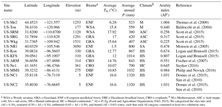
a WSA = Woody savanna, GRA = Grassland, ENF = Evergreen needleleaf forest, DBF = Deciduous broadleaf forest, CRO = croplands; b M = Mediterranean, ASC = Arid steppe cold, SA = sub arctic, HS = Humid subtropical, HC = Humid continental; c AI = P∕Ep (Food and Agriculture Organization, FAO, 2015). We categorized the sites into arid (AI < 0.30), semiarid (0.50 > AI > 0.30), subhumid (0.65 > AI > 0.50), and humid (AI > 0.65) zones, such that each AI category contained at least two validation sites.
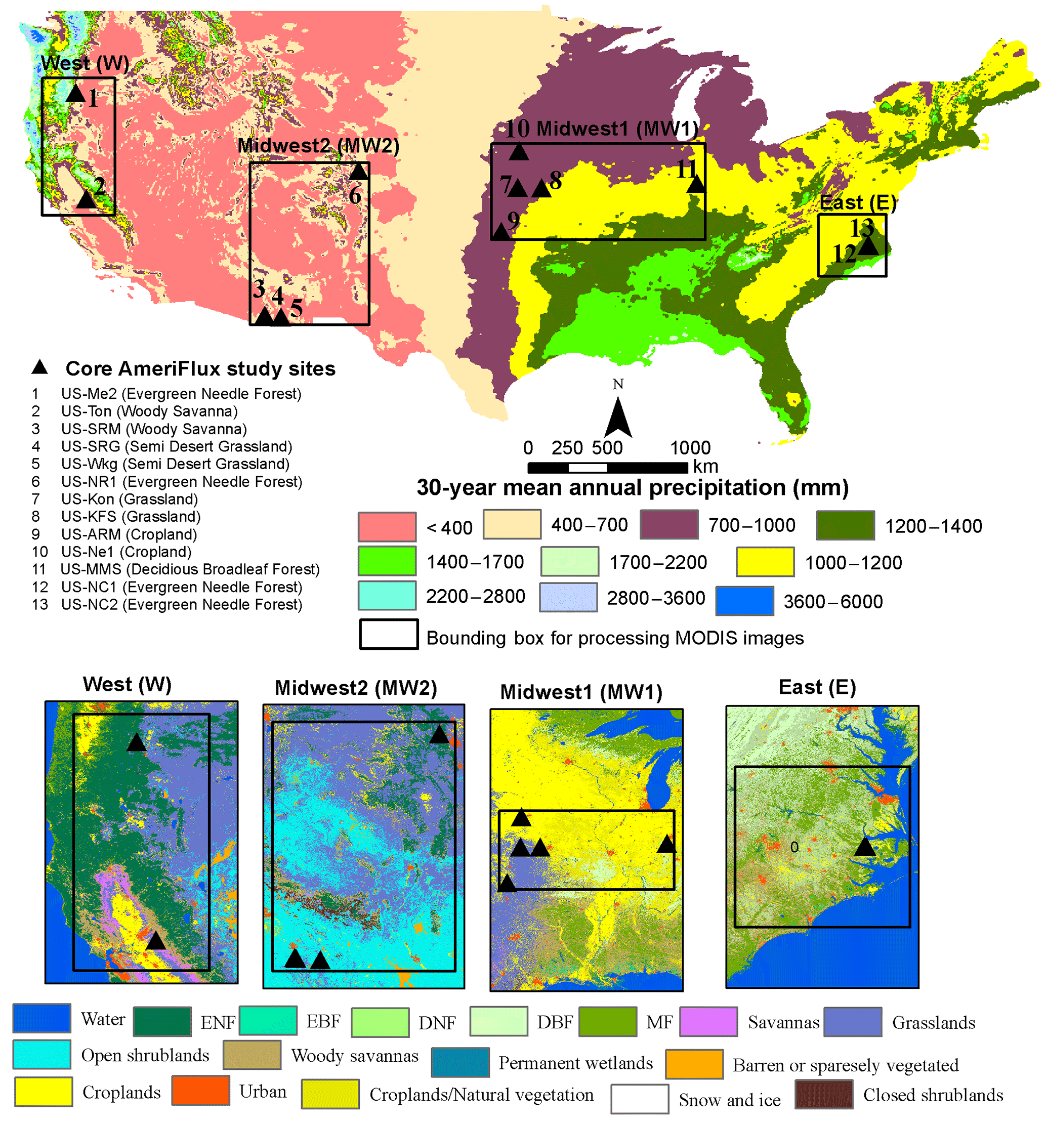
Figure 2Distribution of core AmeriFlux sites (13) used in this study shown over 30-year (1980–2010) mean annual precipitation of the US and the processing grids (MODIS subsets) used to estimate regional-scale ET from MODIS datasets. MODIS land cover maps for each processing grid represents the year 2013 and shows IGBP level 1 classes. EBF, DNF, and MF represent evergreen broadleaf forest, deciduous needle forest, and mixed forest, respectively.
2.1.3 MOD16 algorithm
The MOD16 algorithm is based on the PM equation (Eq. 5) and is designed to estimate ET by summing wet soil evaporation, interception evaporation from the wet canopy, and transpiration through canopy over vegetated land surfaces. The original PM equation was modified by Mu et al. (2007, 2011) for estimating global ET components and is primarily driven by MODIS-derived vegetation variables (leaf area index, LAI; fractional vegetation cover) and daily meteorological inputs including RS, TA, and DA.
Key inputs in the MOD16 ET product include the global 1 km × 1 km MODIS collections, including land cover (MOD12Q1), 8-day LAI/FPAR (MOD15A2), 8-day albedo (MCD43B2 and MCD43B3 products), and the global GMAO daily meteorological reanalysis data (1.00∘ × 1.25∘ resolution). The MODIS 8-day albedo products and daily surface downwelling shortwave radiation and air temperature from daily meteorological reanalysis data are used to calculate RN. The vegetation cover fraction from the MODIS 8-day FPAR products is used to allocate the RN between soil and vegetation. Daily TA, DA, RH, and 8-day MODIS LAI are used to estimate surface stomatal conductance, aerodynamic resistance, wet canopy, and soil heat flux. A biome property lookup table (BPLUT) is used to assign minimum and maximum resistances for all land cover categories, and the biome-specific resistances are constrained by different environmental scalars. Readers are referred to Mu et al. (2011) for a detailed description of the derivation of key ET components and the parameters used in the MOD16 algorithm for estimating ET.
2.2 Study sites
For validating the STIC1.2 model, we selected 13 core AmeriFlux sites covering a broad spectrum of biomes which also represent a wide range of climatic, elevation (5 to 3050 m), precipitation (P; 380 to 1320 mm yr−1), temperature (1.50 to 17.92 ∘C), and aridity gradients across the conterminous United States (Fig. 2; Table 1). AmeriFlux is a subnetwork of FLUXNET, which is a global micrometeorological EC network for measuring carbon, water vapor, and energy exchanges between the biosphere and atmosphere (Baldocchi and Wilson, 2001). AmeriFlux core sites are the EC flux tower sites that deliver high-quality continuous data to the AmeriFlux database (http://ameriflux.lbl.gov). Currently, there are 44 core sites distributed in 12 clusters. We selected 13 out of 44 sites, which also represent the primary EC sites of the selected clusters. These sites also cover a broad class of aridity index (AI; Food and Agriculture Organization, FAO, 2015): arid (AI < 0.30), semiarid (0.50 > AI > 0.30), subhumid (0.65 > AI > 0.50), and humid (AI > 0.65). Each of these four AI categories contained at least two validation sites. Four MODIS subsets (Fig. 2) covering at least two validation sites within each region (labeled as East – E, Midwest1 – MW1, Midwest2 – MW2, and West – W, from the east to west) were used for image processing to implement the STIC1.2 model. For the regional-scale intercomparison of ET models, similar MODIS subsets were used.
2.3 Datasets
Key remotely sensed data for model implementation were obtained from the MODIS Terra 8-day composites. Meteorological inputs were obtained from hourly NLDAS-2 (North American Land Data Assimilation System 2) forcing data (Xia et al., 2012). Daily meteorological variables, which were derived from hourly NLDAS and PRISM (Parameter-elevation Relationships on Independent Slopes Model; PRISM Climate Group, Oregon State University, http://prism.oregonstate.edu) data, were obtained from the University of Idaho (http://climate.nkn.uidaho.edu/METDATA/). A list of datasets used in the present analyses is given in Table 2. The PRISM precipitation dataset was used to select dry, wet, and normal years for each site.
2.4 Data processing
2.4.1 Selection of dry, wet, and normal rainfall years
Dry, wet, and normal years were selected based on 30-year (1980–2010) precipitation from PRISM data. For each site, we selected the driest (dry), wettest (wet), and closest to the 30-year mean (normal) years based on PRISM precipitation data (Fig. 3).
Table 2Descriptions of MODIS and meteorological datasets used in this study.
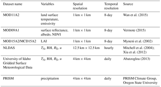
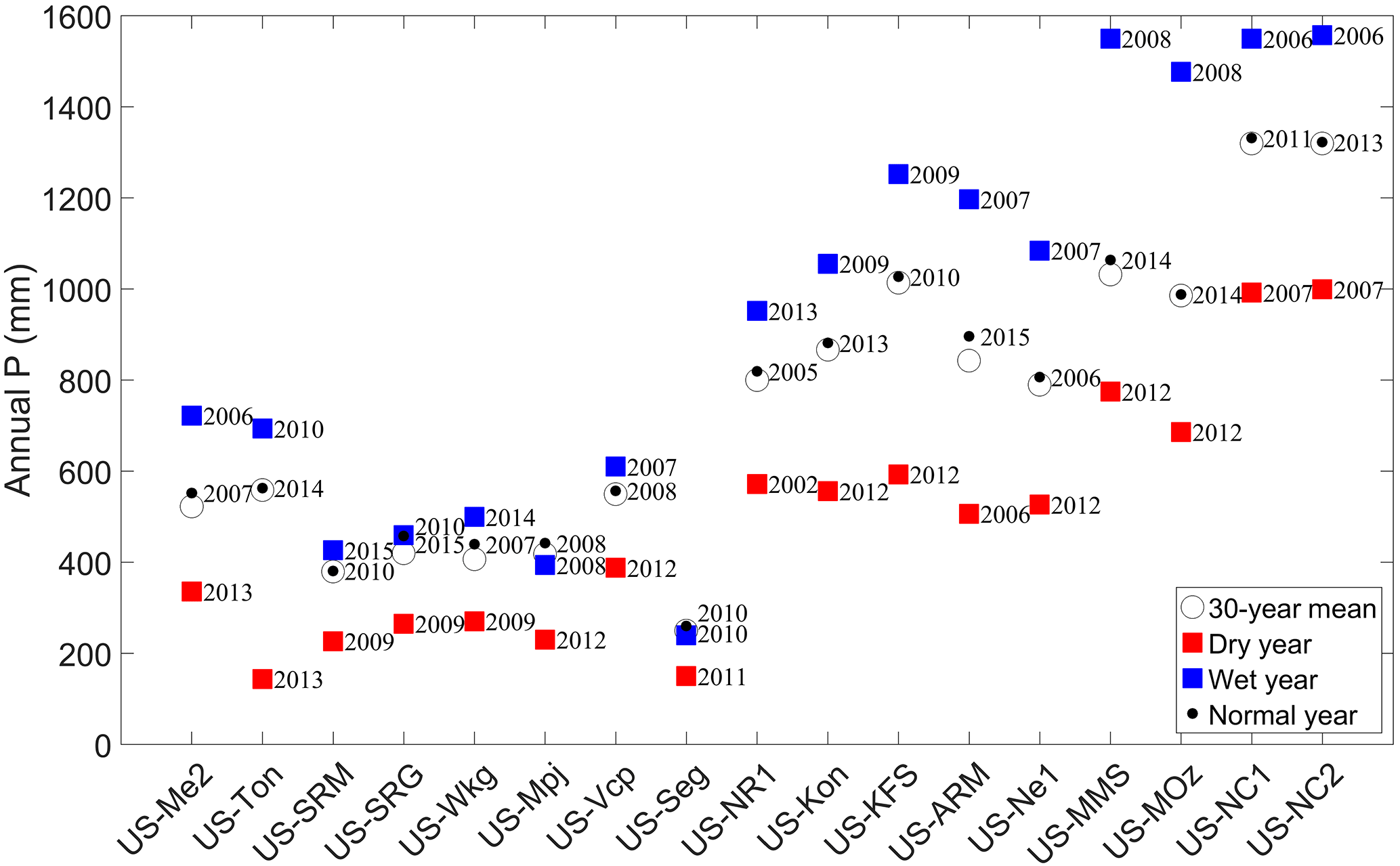
Figure 3Distribution of annual precipitation (P) during dry, wet, and normal years considered for ET evaluation at each site corresponding to its 30-year mean annual precipitation from the PRISM data.
2.4.2 MODIS-based variables: surface albedo, NDVI, LST, surface emissivity, and LAI
Broadband surface albedo was estimated using all the narrow band surface reflectances from MOD09A1, and NDVI (Tucker, 1979) was computed using near-infrared and red band surface reflectance of MOD09A1 products. TR information was obtained from the MOD11A2 LST product for the study years. For estimating surface emissivity, we took mean emissivity from bands 31 and 32 (Bisht et al., 2005) from the MOD11A2 products. While the information for LAI from MOD15A2 and MCD15A2 products (mean of the two) were used for computing the extra resistance parameter (kB−1) (Su, 2002; Su et al., 2001). NDVI was used to estimate z0M using a simple empirical relationship between the roughness length of momentum transfer (van der Kwast et al., 2009) in SEBS. Yang et al. (2002) was used to parameterize kB−1 for bare soil. This new parameterization of kB−1 was designed to improve the SEBS model performances on bare soil, low canopies, and snow surfaces, and was proposed by Chen et al. (2013).
2.4.3 Meteorological variables at the satellite overpass: RH, TA, u, and RS
Half-hourly gridded meteorological datasets from the North American Land Data Assimilation System (NLDAS-2) at 4 km × 4 km spatial resolution were used as inputs in the STIC1.2 (RS, TA, and RH) and SEBS (u, RS, TA, and RH) models. Because RH was not explicitly available in the NLDAS-2 dataset, we derived RH from surface pressure (Pa) and specific humidity (kg kg−1) information using the method developed by McIntosh and Thom (1978). The half-hourly meteorological variables at the time of MODIS Terra overpass during every 8-day period were averaged to ensure that the weather dataset is well representative of all the corresponding 8 days within each MODIS 8-day period. Additional inputs of daily meteorology (RS, TA, u, and RH) required for computing 8-day ET were obtained from the University of Idaho (http://climate.nkn.uidaho.edu/METDATA/), and these data products were derived from hourly NLDAS and PRISM datasets. Daily weather data were also aggregated to the corresponding MODIS 8-day periods.
2.4.4 Derivation of regional-scale 8-day and annual ET maps (STIC1.2 and SEBS)
The SEBS code in this study is adapted from Abouali et al. (2013), which is different from original and modified versions of Su (2002) and Chen et al. (2013), respectively. Here we used a simple NDVI-based parameterization of z0M to provide a spatial representation of canopy height (z0M∕0.13) and zero displacement height (0.67z0M) and zOH was estimated using Eq. (14). The STIC1.2 source code was modified from the original STIC1.2 code (Mallick et al., 2016) in Matlab (Mathworks Inc, Natick, USA).
Net available energy (ϕ = RN − G, W m−2) at MODIS Terra overpass time was partitioned into H and λE by both models as explained in Sects. 2.1.1 and 2.1.2. Instantaneous Λ was then computed as the ratio of λE to ϕ. For the extrapolation of instantaneous λE to daily ET under clear sky conditions, the instantaneous Λ is assumed to be constant for the day (Brutsaert and Sugita, 1992; Crago and Brutsaert, 1996) and 8-day cumulative ET (5-day for DOY 361) was estimated as follows:
where RN24-8day is the 8-day net radiation; and n is the number of days in the 8-day period (8; n = 5 for DOY 361) computed using the ASCE standardized PM equation using daily weather inputs (ASCE-EWRI, 2005). Combining all the sites, the estimated RN24-8day from MODIS was within 10 % (i.e., 9 % overestimation) of mean observed 8-day net radiation at the flux sites (coefficient of determination, R2, = 0.89, root mean squared error, RMSE, = 20 W m−2; Fig. S1).
Annual ET maps were derived by summing all the corresponding 8-day ET maps within a given year. To fill the missing 8-day ET values, Λ values from up to the two nearest 8-day periods were used (i.e., mean Λ values of n prior and after 8-day period, where n = 1 or 2). The filled Λ values were then used in Eq. (17) (RN24-8day from the current 8-day period is used) to fill the missing 8-day ET values. Since there were missing daily flux data in some years, we filled missing values using linear interpolation between available days. For the statistical analysis, we retained those annual ET values when observed λE was available for at least 300 days at each flux tower site. Similarly, annual ET from the models was only compared when at least 38 (out of the 46) 8-day cumulative ET values were available.
2.4.5 Regional-scale 8-day and annual ET maps from MOD16 ET
The MOD16 ET product provides global 8-day (MOD16A2), monthly, and annual (MOD16A3) terrestrial ecosystem evapotranspiration datasets at 1 km × 1 km spatial resolution over 109.03 million km2 of global vegetated land areas. The dataset is currently available for the period of 2000–2014 and will be updated for years beyond 2014 in the future. The 8-day and annual MOD16 ET products were acquired from the Numerical Terradynamic Simulation Group (ftp://ftp.ntsg.umt.edu/pub/MODIS/NTSG_Products/MOD16/MOD16A2.105_MERRAGMAO/) of the University of Montana. ET values of the corresponding flux sites for every 8-day period within each dry, wet, and normal year were extracted for model intercomparison. The annual ET maps from MOD16 products (MOD16A3) were used for regional-scale model intercomparison of annual ET estimates from STIC1.2 and SEBS.
2.4.6 Preparation of validation datasets
We used half-hourly SEB flux data from the 13 core EC sites of the AmeriFlux network that covers an aridity gradient (from arid to humid), and a wide range of elevation and biome types in the conterminous US (Table 1). A Bowen-ratio-based (Bowen, 1926) SEB closure method (Chávez et al., 2005; Twine et al., 2000) was used to force the SEB closure at half-hour timescales. The half-hourly λE (W m−2) was converted into ET (mm h−1) using the proportionality parameter between energy and equivalent water depth unit of ET (Mu et al., 2007; Velpuri et al., 2013).
Here λ is the latent heat of vaporization of water.
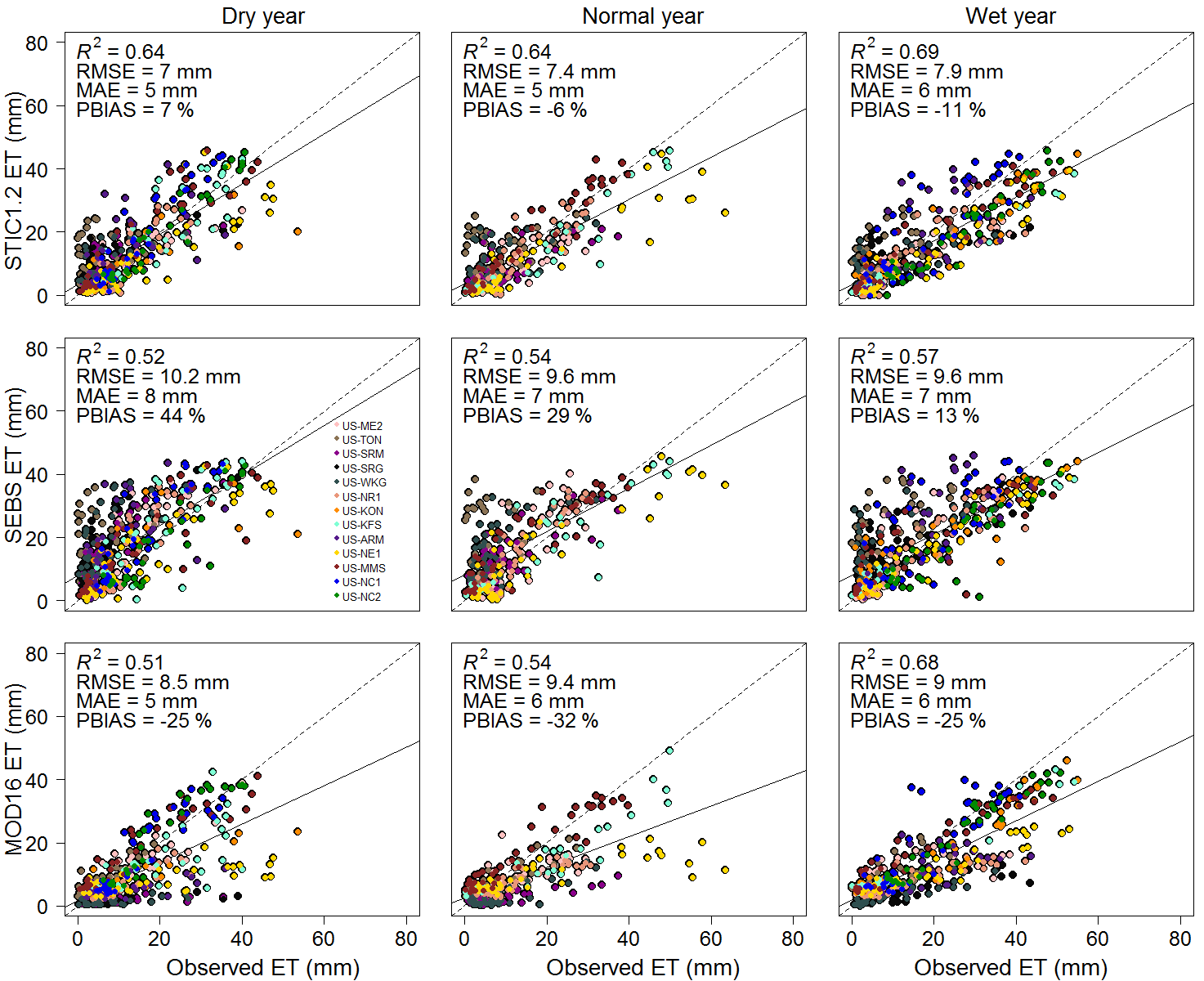
Figure 4Evaluation of 8-day cumulative ET from STIC1.2, SEBS, and MOD16 against observed ET from 13 core AmeriFlux sites in the US during dry, wet, and normal years.
Half-hourly ET were aggregated to hourly, daily, and 8-day timescales corresponding to the MODIS 8-day periods. The 8-day sum of ET was used for validating ET estimates from MOD16, SEBS, and STIC1.2 only when flux data were available for the entire 8-day period. Daytime fluxes (H, λE, RN, and G) close to the MODIS Terra overpass time were also averaged over 8-day periods corresponding to MODIS 8-day DOYs. We also utilized a recently developed global monthly ET product (5 km × 5 km; http://en.tpedatabase.cn/portal/MetaDataInfo.jsp?MetaDataId=249454) that employs the latest version of SEBS (SEBSChen hereafter; Chen et al., 2013, 2014) and compared against those from STIC1.2 outputs. SEBSChen uses an updated parameterization of the kB−1 parameter through improved canopy height and surface roughness schemes to better represent surfaces from bare soil to full canopies in SEBS. Since the focus of this study is to test the validity of the regional-scale implementation and ET mapping potential of STIC1.2 using remotely sensed data, a detailed model intercomparison or assessing the performances of SEBS model with different kB−1 parameters or input variables is beyond the scope of this study.
2.4.7 Statistical analysis
The three ET models were evaluated based on their ability to estimate 8-day cumulative ET at the flux tower sites during dry, normal, and wet years. Widely used statistical metrics, such as RMSE, R2, mean absolute error (MAE), and percent bias error (PBIAS) were used for evaluating the model performances. The location information of the AmeriFlux sites (Table 1) was used to extract the pixel values of ET (outputs from STIC1.2, SEBS, and MOD16 products) and other biophysical variables (Table 2) for the statistical analysis.
Comparisons were made for the 8-day periods when flux data were available for all 8 days corresponding to each MODIS 8-day period, and when MODIS inputs for STIC1.2, SEBS, and MOD16 ET data were available. Overall, the data available for statistical analysis ranged from 43 % (59 out of 138 MODIS 8-day periods) at the US-kon site to 93 % (128 out of 138 MODIS 8-day periods) at the US-Wkg site with an average of 65 % (Table S1 in the Supplement).
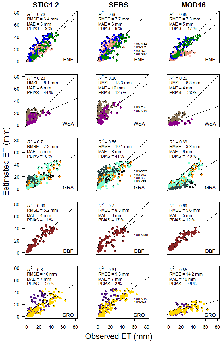
Figure 5Validation of 8-day cumulative ET from STIC1.2, SEBS, and MOD16 for each biome type.
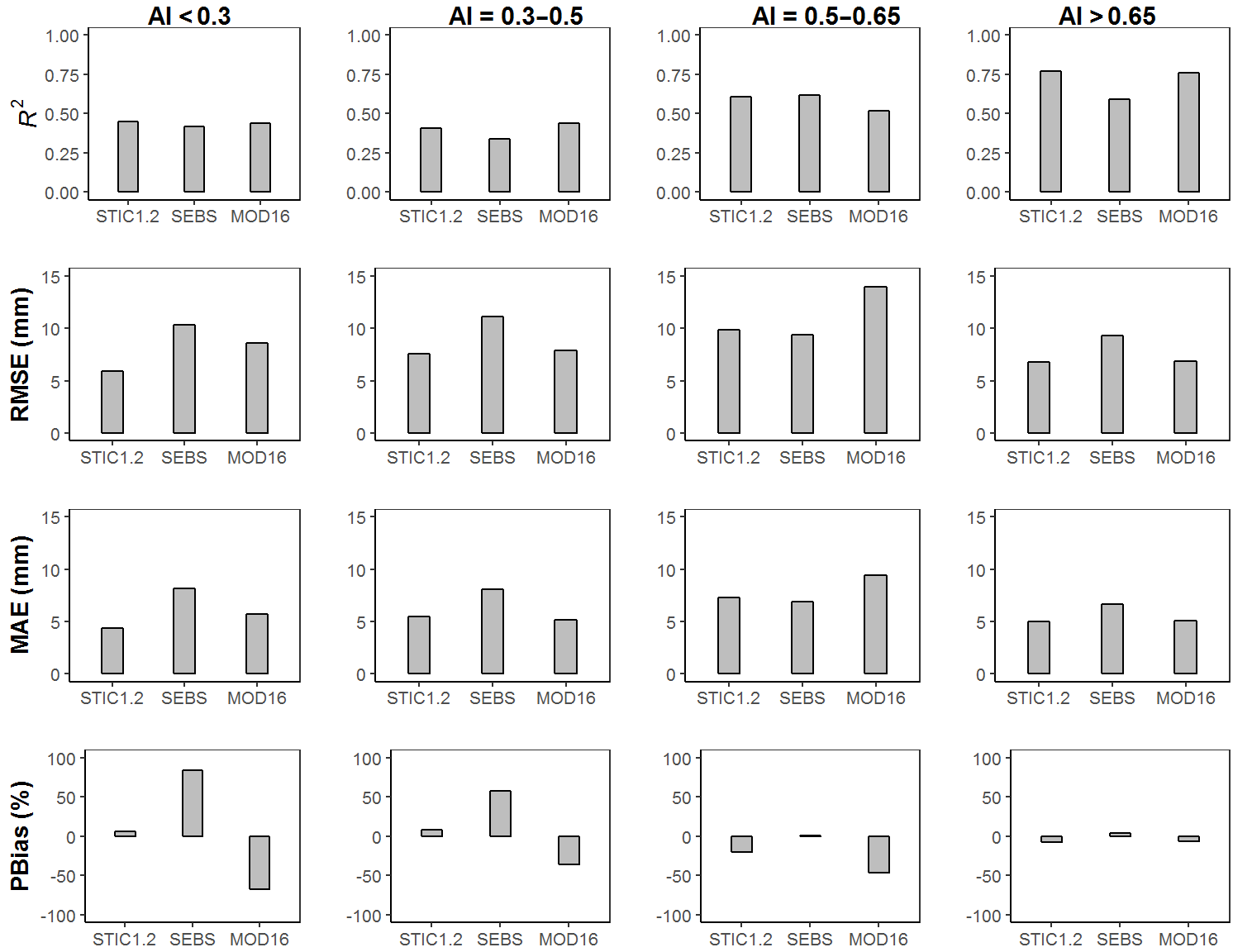
Figure 6Evaluation of 8-day cumulative ET from STIC1.2, SEBS, and MOD16 for each long-term aridity index (AI) category.
3.1 What is the performance of STIC1.2 at the regional-scale across an aridity gradient and during contrasting rainfall years in the conterminous US?
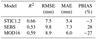
Combining results from 13 core AmeriFlux sites, it is apparent that STIC1.2 captured 66 % of the observed variability (R2 = 0.66) in 8-day cumulative ET (Table 3) with an overall RMSE, MAE, and PBIAS of 7.5 mm, 5.4 mm, and −3 %, respectively. Consistent performance of STIC1.2 was noted throughout dry, wet, and normal rainfall years, explaining about 64–69 % of the variability in 8-day cumulative ET (Fig. 4), with a slight overestimation in dry years (PBIAS 7 %) and an underestimation in wet years (PBIAS −11 %; Fig. 4). Biome-specific analysis revealed relatively better performance of STIC1.2 in forests as compared to non-forest sites (Fig. 5). STIC1.2 explained 73–89 % variability in ET from ENF (evergreen needleleaf forests) and DBF (deciduous broadleaf forests) with an RMSE of 5.2–6.4 mm. Among the non-forest sites, although STIC1.2 explained 60–70 % of the observed ET variability in CRO (croplands) and GRA (grasslands) (RMSE of 7.2–9.9 mm/8-day), it explained only 23 % of the observed ET variability in WSA (woody savanna) with a PBIAS of 44 % (Fig. 5).
At the CRO sites, STIC1.2 underestimated ET by about 20 %. At the GRA sites, a better performance of STIC1.2 was noted in the dry year as compared to the wet and normal years (Figs. S2–S4). Regardless of vegetation type, STIC1.2 had a tendency to underestimate ET under high wetness conditions.
Table 3Evaluation of 8-day cumulative ET from STIC1.2, SEBS, and MOD16 against observed ET from 13 core AmeriFlux sites in the US combining data from one dry, one wet, and one normal year.
Performance evaluation of STIC1.2 across an aridity gradient suggests the better predictive capacity of STIC1.2 in subhumid and humid sites as compared to arid and semiarid sites (Fig. 6). As seen in Fig. 6, 41–45 % of the variability in 8-day ET was explained in arid and semiarid ecosystems (RMSE of 5–7.5 mm/8-day and MAE 4.8–5.1 mm/8-day), which increased to 61–77 % in the humid and subhumid ecosystems (with RMSE of 7–10 mm/8-day and MAE of 5–7.5 mm/8-day). The key reason is that STIC1.2 does not effectively capture very low ET values in the semiarid and arid sites, particularly in woody savannas (Fig. 5).
3.2 Comparison of STIC1.2 against other global ET models that are constrained by TR and RH
STIC1.2 showed relatively high accuracy when independently compared against observed ET at 13 AmeriFlux sites than did SEBS and MOD16. Combining all sites, the predictive capability of STIC1.2 was found to be 7–17 % better than SEBS and MOD16, which explained about 53 and 59 % of the variability in observed 8-day ET, respectively (Table 3). As evident from PBIAS, SEBS has a tendency to overestimate and MOD16 has a tendency to underestimate 8-day cumulative ET by over 20 % (28 % from SEBS and −27 % from MOD16), while STIC1.2 has a small tendency to underestimate (−3 %) (Table 3). In addition to a high RMSE (9.6–10.2 mm for SEBS, 8.5–9.4 mm for MOD16), an overestimation tendency of SEBS (PBIAS 13–44 %) and underestimation tendency of MOD16 (PBIAS −25 to −32 %) were consistent throughout dry, wet, and normal years (Fig. 4).
The biome-specific performance intercomparison revealed that STIC1.2 produced a substantially lower RMSE than SEBS and MOD16 in ENF (12–17 % less RMSE), GRA (18–29 % less RMSE), and DBF (7–37 % less RMSE) in 8-day cumulative ET with better or tantamount skill in capturing the observed ET variability as compared to the two other models (Fig. 5). While MOD16 was found to produce relatively lower RMSE in WSA (16 % less than STIC1.2 and 49 % less than SEBS), SEBS performed relatively better in CRO (5 and 33 % less RMSE than STIC1.2 and MOD16, respectively).

Figure 7Scatter plots of differences in STIC1.2 and (a–c) SEBS and (d–f) MOD16 ET estimates against input land surface variables used in these models (TR, DA, and NDVI). The Pearson correlation coefficient, r (p-value was < 0.005 for all cases except dETMOD16-obs vs. NDVI relationship), is also shown in each plot.
Statistical intercomparison of the predictive capacity of STIC1.2 with respect to SEBS and MOD16 across an aridity gradient revealed notable differences in RMSE and MAE between the models (Fig. 6), despite general agreement on the capabilities of individual models to explain the variability in observed ET (R2 = 0.34–0.77). STIC1.2 was found to produce the lowest RMSE in 8-day cumulative ET in arid (31 and 43 % lower than MOD16 and SEBS, respectively), semiarid (5 and 32 % lower than MOD16 and SEBS, respectively), and humid (3 and 19 % lower than MOD16 and SEBS, respectively) ecosystems (Fig. 6). In the subhumid ecosystem, the performance of STIC1.2 was comparable with SEBS (PBIAS from STIC1.2 and SEBS were −20 and 2 %, respectively, and other error statistics were comparable) and substantially better than MOD16 (PBIAS = −48 %). A consistent overestimation (underestimation) tendency of SEBS (MOD16) in arid and semiarid ecosystems is reflected the in positive (negative) PBIAS (58 to 84 % for SEBS, −67 to −37 % for MOD16) in these two aridity classes.
3.3 Factors affecting agreements or disagreements between ET models
The residual differences in 8-day ET between STIC1.2 vs. SEBS (dETSTIC1.2-SEBS = ETSTIC1.2 − ETSEBS) as well as SEBS vs. observed ET (dETSEBS-obs = ETSEBS − ETobs) were found to be significantly associated with TR (r = −0.301 to 0.38, p-value < 0.005) and DA (r = −0.30 to 0.46, p-value < 0.005) (Fig. 7a and b). Negative dETSTIC1.2-SEBS (positive dETSEBS-obs) was found with increasing TR and DA above 290 K and 2 kPa, whereas ET differences were narrowed down below these limits (Fig. 7). A logarithmic pattern was found between dETSTIC1.2-SEBS (dETSEBS-obs) and NDVI, with a correlation of 0.31 and 0.35, respectively. Major ET differences (both dETSTIC1.2-SEBS and dETSEBS-obs; ±20 mm) were found in the NDVI range of 0.15–0.35, whereas ET differences were diminished within ±10 mm above NDVI of 0.5.
A similar analysis of ET differences between STIC1.2 and MOD16 (dETSTIC1.2-MOD16 = ETSTIC1.2 − ETMOD16) and between MOD16 and the observed ET (dETMOD16-obs = ETMOD16 − ETobs) also revealed a significant correlation with TR and DA (Fig. 7d, e and inset; r = −0.30 to 0.66, p-value < 0.005), but the direction of these correlations are opposite to those found with the ET differences between STIC1.2 and SEBS. dETMOD16-obs was found to have no significant relationship (p-value > 0.15) with NDVI, while dETSTIC1.2-MOD16 appears to have a significant negative relationship with NDVI, which was also opposite of what was found in ET differences between STIC1.2 and SEBS.
To examine the relative importance of the meteorological and land surface variables in explaining the variances in dETSTIC1.2-SEBS and dETSTIC1.2-MOD16, a random forest analysis (Liaw and Wiener, 2002) was performed between the residual ET differences and seven climatic/land surface variables (NDVI, DA, P, u, observed soil moisture – SM, TA, and TR) as predictors (Fig. S5). Overall, these variables explained 41 and 57 % of variances in dETSTIC1.2-SEBS and dETSTIC1.2-MOD16, respectively. The most important variables for explaining variance in dETSTIC1.2-SEBS were TA and NDVI. These two variables would lead to about 25–40 % increase in mean residual errors (MSEs) if they are permuted in the random forest model. For dETSTIC1.2-MOD16, all the variables expect u appeared to be important in determining the variance in ET difference, as each variable would lead to about 17–22 % increase in MSEs if they are permuted in the random forest model.
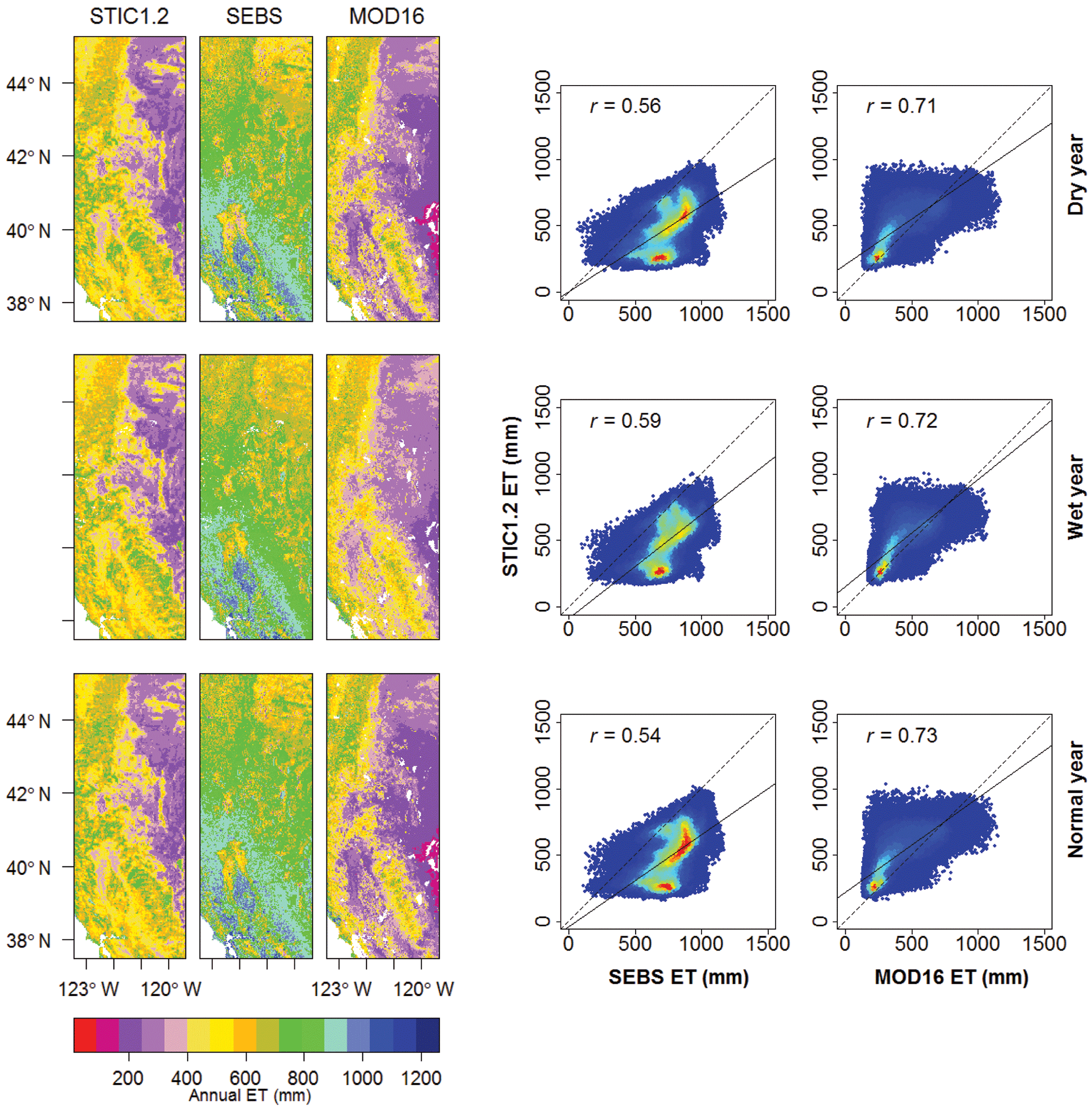
Figure 8Annual ET (mm) maps for the dry, wet, and normal years derived from STIC1.2, SEBS, and MOD16 for the western (W) bounding box covering US-Ton and US-Me2 flux sites (Fig. 1). Scatter plots between annual ET estimates from STIC1.2 vs. SEBS and MOD16 are shown on the right.
3.4 Regional-scale intercomparison of STIC1.2 vs. SEBS and MOD16 ET
Annual ETs from STIC1.2 for the driest, wettest, and normal precipitation years for each of four study zones during the period 2001–2014 were compared against those derived from SEBS and the MOD16A3 annual ET products. Because the study years were selected based on the spatial mean of precipitation across 4 km × 4 km PRISM grids, the study years (Table 4) do not necessarily match with those considered for ET analysis over the flux sites as presented in Sects. 3.1–3.3.
Figures 8–11 present annual ET maps for the driest, wettest, and normal years for each of the four study zones covering all 13 study sites and a distinct positive relationship was found between annual ET computed from the three models. However, the magnitude of annual ET from the three models varied widely, particularly in the relatively dry zones of the midwestern US (MW1 and MW2). Such differences in annual ET could be attributed to the systematic differences in 8-day cumulative ET among the three models (i.e., overestimation from SEBS and underestimation from MOD16).
Table 4Study years considered for regional-scale intercomparison of annual ETs from STIC1.2, SEBS, and MOD16.
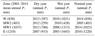

Figure 9Annual ET (mm) maps for the dry, wet, and normal years derived from STIC1.2, SEBS, and MOD16 for the Midwest2 (MW2) bounding box covering US-ARM, US-SRG, US-Wkg, and US-NR1 flux sites (Fig. 1). Scatter plots between annual ET estimates from STIC1.2 vs. SEBS and MOD16 are shown on the right.

Figure 10Annual ET (mm) maps for the dry, wet, and normal years derived from STIC1.2, SEBS, and MOD16 for Midwest1 (MW1) bounding box covering US-Kon, US-KFS, US-ARM, US-Ne1, and US-MMS flux sites (Fig. 1). Scatter plots between annual ET estimates from STIC1.2 vs. SEBS and MOD16 are shown on the right.
Table 5Mean percentage difference in annual ET (standard deviation in parentheses) between STIC1.2 vs. SEBS and MOD16 from all pixels within the bounding box of four study zones during dry, wet, and normal years.
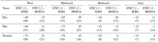
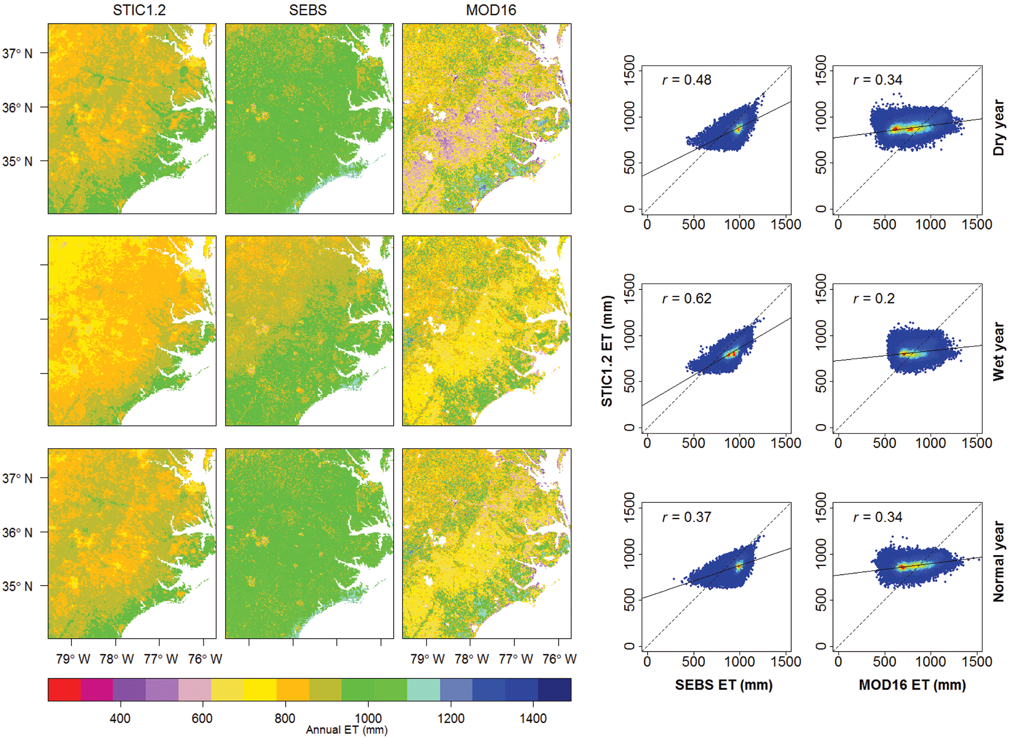
Figure 11Annual ET (mm) maps for the dry, wet, and normal years derived from STIC1.2, SEBS, and MOD16 for the eastern (E) bounding box covering US-NC1 and US-NC2 flux sites (Fig. 1). Scatter plots between annual ET estimates from STIC1.2 vs. SEBS and MOD16 are shown on the right.
The mean percent difference (and standard deviation) in ET between STIC1.2 vs. SEBS and MOD16 (Table 5) from all pixels within the bounding box of four study zones during the contrasting rainfall years (as in Figs. 8–11) showed noteworthy disagreements in arid and semiarid (W and MW2) zone, where annual ET from SEBS (MOD16) were 66–85 % more (11–55 % less) than STIC1.2. Conversely, major agreements between the models were found in the humid (E) zone where SEBS and MOD16 annual ET estimates were within 13 % of STIC1.2 ET.
We further compared annual ET estimates from the models against the flux tower estimates for the years listed in Table 5 and annual ET maps corresponding to Figs. 8–11. Comparison of annual ET at the core AmeriFlux sites revealed a consistent overestimation and underestimation from SEBS (PBIAS 23 %) and MOD16 (PBIAS −30 %) (Fig. 12). STIC1.2 produced the lowest RMSE (175 mm) and MAE (134 mm) as compared to SEBS (RMSE 239 mm, MAE 188 mm) and MOD16 (RMSE 261 mm, MAE 228 mm) and was comparable with annual ET estimates from SEBSChen (sum of monthly ET maps), with respect to RMSE and MAE (Fig. 12). Biases from STIC1.2 was better (PBIAS = −6 %) than SEBSChen (−14 %) although STIC1.2 only explained 32 % variation in observed annual ET, while SEBSChen explained about 56 % variability in observed annual ET.
Table 6Mean percent difference in annual ET (standard deviation in parentheses) between STIC1.2 vs. SEBS and MOD16 within the bounding box of the four study zones considering all pixels and five vegetation types based on MCD12Q1 products (Friedl et al., 2010). NA = not available.
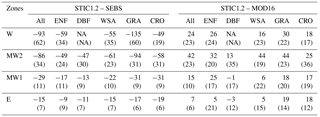
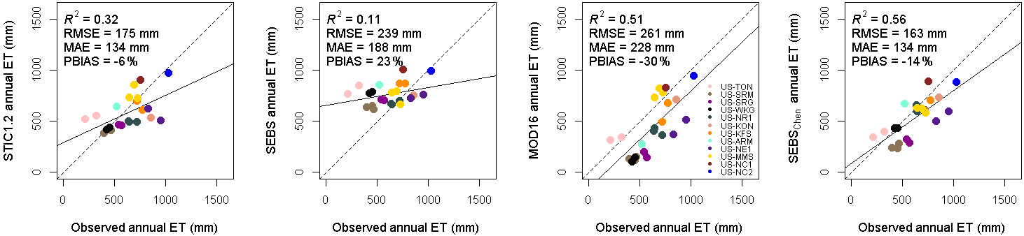
Figure 12Comparison of annual ET from STIC1.2, SEBS, MOD16, and SEBSChen against observed annual ET from the core AmeriFlux sites. Missing daily observed ET at the flux sites were filled using linear interpolation between available days. Missing 8-day cumulative ET from STIC1.2 and SEBS were filled using the constant evaporative fraction (EF) approach. Annual ET from the models and flux sites are compared when at least 38 (out of 46) 8-day cumulative ET were available for computation of annual ET and at least 300 days of observed λE were available at the flux tower sites. SEBSChen is a recently developed global monthly SEBS ET product based on improved kB−1 parameterization outlined in Chen et al. (2013).
Figure 12 provides evidence that errors in 8-day cumulative ET from SEBS and MOD16 were largely additive, as indicated by the consistent overestimation or underestimation from the models at different sites. In addition, the 8-day average net radiation was also overestimated by about 9 % (Fig. S1). Overestimation of annual ET from SEBS was mostly observed in the arid and semiarid sites (47 %). In the two cropland sites (US-ARM and US-Ne1), SEBS annual ET estimates were within 2 % of observed annual ET, where STIC1.2 showed 22 % underestimation and MOD16 revealed 49 % underestimation. Notably, MOD16 estimates were particularly poor in the MW2 zones, while SEBS was found to be poor both in the MW1 and MW2 zones. Apart from that, differences between STIC1.2 and the other two models were also noticed in other zones.
To further investigate the role of biomes on ET differences between STIC1.2 and other models, we computed the mean percent ET difference (standard deviation, similar to Table 5) on the five vegetation types, corresponding to those represented by the core AmeriFlux sites. The differences in annual ET between STIC1.2 vs. SEBS and STIC1.2 vs. MOD16 were mostly evident in all five vegetation classes, particularly in the W and MW2 spatial domains, with the maximum ET differences in grasslands (−135 to 44 %; Table 6). For almost all of the five vegetation types, ET differences between the models decreased across the aridity gradient from arid to humid ecosystems from western to the eastern US (±20 %; Table 6).
In order to quantify the relative contribution of these three categorical variables – e.g., (1) zones (W, MW2, MW2, E), (2) land cover types (five land cover classes), and (3) precipitation extremes (dry, wet, and normal years) – to variations in residual ET differences (annual) between STIC1.2 and the other two models, we performed a random forest analysis (Fig. S6). The three categories together explained 45 to 60 % of the variances in the residual ET difference between STIC1.2 vs. MOD16 and STIC1.2 vs. SEBS. However, study zone increases of 51–65 % in mean residual errors (MSEs) in ET if this group is permuted in the random forest model, thus appearing to be the most important factor among the three categorical variables. This finding is also consistent with the results presented in Tables 5 and 6 that the residual ET differences between the models progressively reduced across an aridity gradient from arid to humid ecosystems. The precipitation extremes appeared to have no effect on the residual ET difference between STIC1.2 and SEBS, similar to the land cover effect on the residual difference between STIC1.2 and MOD16.
Overall, STIC1.2 performed reasonably well across an aridity gradient and a wide range of biomes in the conterminous US. One noticeable weakness of STIC1.2 appears to be its tendency to underestimate ET in grassland and cropland land cover types (Figs. 4 and 5). These biases could be attributed to the nature of the MODIS LST product that aggregates sub-grid heterogeneity in TR, vegetation cover, and radiation at 1 km × 1 km area. Due to the relatively low tower heights in CRO and GRA sites (3–10 m), the EC towers aggregate fluxes at scales of approximately 0.009–0.10 km2. Such a critical mismatch of the scales between MODIS pixels and the flux tower footprint could be a potential source of disagreement between STIC1.2 and tower-observed ET (Stoy et al., 2013). Another source of error could be the presence of widely varied dry and wet patches within one MODIS 1 km × 1 km pixel as well as around the flux towers. For example, if more than 50 % of the area falling within a 1 km × 1 km MODIS pixel is predominantly dry, the lumped TR signal in MODIS LST product will be biased due to the dryness of the landscape (Stoy et al., 2013; Mallick et al., 2014, 2015) and the resultant ET will be underestimated. The overestimation tendency in WSA is mainly due to the poor performance of STIC1.2 in the Tonzi Ranch site (US-Ton), which could be associated with the uncertainties in surface emissivity correction and systematic underestimation of MODIS LST in arid and semiarid ecosystems (Wan and Li, 2008; Jin and Liang, 2006; Hulley et al., 2012). Since TR plays an important role in constraining the conductances in STIC1.2, an underestimation of TR would result in an overestimation of gC and underestimation of gA, which would result in overestimation of ET. The differences between STIC1.2 vs. observed ET in WSA may also largely be attributed to the Bowen ratio energy balance closure correction of EC λE observations (Chávez et al., 2005; Twine et al., 2000). Although the Bowen ratio correction forces SEB closure, in arid and semiarid ecosystems major corrections are generally observed in sensible heat flux, whereas λE is negligibly corrected (Chávez et al., 2005; Mallick et al., 2018). Besides, direct water vapor adsorption on the land surface occurs in arid and semiarid ecosystems when air close to the surface is drier than the overlying air (McHugh et al., 2015; Agam and Berliner, 2006), and this source of moisture is unaccounted for in the EC measurements. This will automatically result in a disagreement between STIC1.2 and observed ET. Nevertheless, the performance of STIC1.2 in forest ecosystems is encouraging, given the uncertainties associated with more complex SEB models that use MOST to parameterize the turbulent mixing in tall canopies (Finnigan et al., 2009; Garratt, 1978; Harman and Finnigan, 2007) that could induce substantial biases in estimated fluxes (Wagle et al., 2017; Numata et al., 2017; Bhattarai et al., 2016).
The overall performance metrics from the three models may be slightly biased due to their strikingly poor performances at some specific sites (Table S1). For example, although SEBS overestimated ET by over 64 % in the two semiarid WSA (US-Ton, US-SRM) and GRA (US-SRG and US-Wkg) sites (Table S1), its performance in US-Ne1 (CRO), two wet grasslands (US-Kon and US-KFS), and US-NR1 (ENF) were better or comparable than the other two models. This could be due to the inability of the kB−1 parameterization scheme in SEBS to account for the substantial differences between TR and T0 due to strong soil water limitations. MOD16 underestimated ET from all but three sites (US-Ton, US-MMS, US-NC1) and underestimated mean ET by over 50 % in US-Ne1 (CRO), US-SRM (WSA), US-SRG (GRA), and US-Wkg (GRA) sites. STIC1.2 appears to be relatively consistent among the three models, as the mean bias errors were within 20 % for all but three sites (US-Ton, US-Kon, US-Ne1).
Performance intercomparison of STIC1.2 with SEBS and MOD16 indicated overall low statistical errors for STIC1.2, and better agreement than SEBS and MOD16 with observed ET values. The principal differences between STIC1.2 and SEBS (as evident from Figs. 7a and 8–13), in particular the overestimation of ET through SEBS, is in cases of high TR and DA with low vegetation cover (i.e., low NDVI), a characteristic feature of arid and semiarid ecosystems. In these water-limited ecosystems, TR induced water stress and the diminishing ET rate leads to high atmospheric dryness (i.e., high DA), increased evaporative potential, and very high sensible heat flux. This leads to substantial differences between TR and T0, and the role of radiometric roughness length (z0H) becomes critical, which is estimated empirically through the adjustment factor kB−1 (Paul et al., 2014). Although there is a first order dependence of kB−1 on TR, radiation, and meteorological variables (Verhoef et al., 1997a), no physical model of kB−1 is available (Paul et al., 2014). Therefore, uncertainties in kB−1 estimation are propagated into z0H. Overestimation (or underestimation) of z0H would lead to underestimation (overestimation) of gA in SEBS, which is mirrored in ET differences between SEBS vs. observations (dETSEBS-obs; Zhou et al., 2012). This is also evident when a logarithmic pattern was found between dETSEBS-obs and kB−1, with a correlation of 0.39 (p-value < 0.005; Fig. 13a). Major ET differences were found (±20 mm) within a kB−1 range of 2–6 (arid, semiarid, heterogeneous vegetation), whereas ET differences were diminished within ±10 mm above kB−1 of 6 (subhumid, humid, homogeneous vegetation). Apart from z0H, empirical parameterization of z0M and a resultant ±50 % uncertainties in z0M can also lead to 25 % errors in gA estimation (Liu et al., 2007; Verhoef et al., 1997a), which will lead to more than 30 % uncertainty in ET estimates. This is also evident from the exponential scatter between z0M and dETSEBS-obs (Fig. 13b) that showed a significant negative correlation between z0M and the residual ET error (r = −0.40, p-value < 0.005).
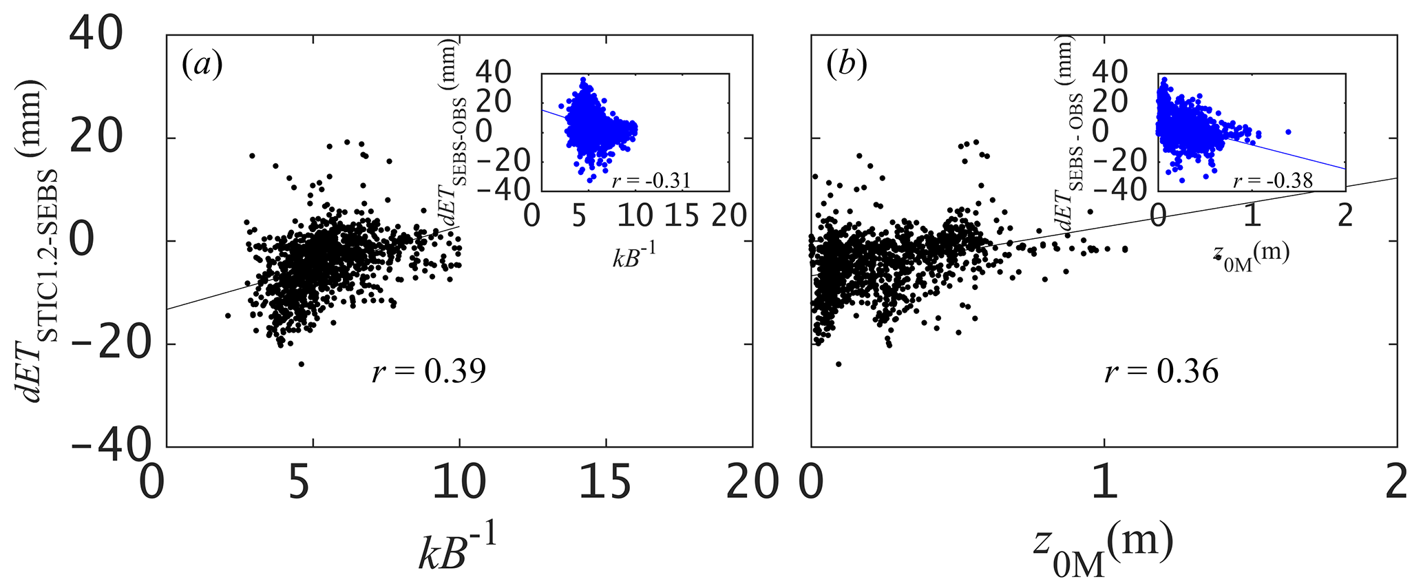
Figure 13Scatter plots of the residual differences in cumulative 8-day ET estimates from STIC1.2 and SEBS and the residual errors from SEBS (vs. the observations) against kB−1 and z0M. Pearson correlation coefficient, r (p-value was < 0.005 for all relationships shown above), are also shown in each plot. The z0M was estimated from NDVI (van der Kwast et al., 2009) using no prior canopy height information.
It is important to emphasize that the momentum transfer equation for estimating gA in SEBS is based on the semi-empirical MOST approach that mainly holds for extended, uniform, and flat surfaces (Foken, 2006; Verhoef et al., 1997b). MOST tends to become uncertain on rough surfaces due to a breakdown of the similarity relationships for heat and water vapor transfer in the roughness sub-layer, which results in an underestimation of the “true” gA by a factor of 1–3 (Holwerda et al., 2012; van Dijk et al., 2015a; Simpson et al., 1998). Since gA is the main anchor in SEBS, an underestimation of gA would lead to an underestimation of sensible heat flux and an overestimation of ET (Gokmen et al., 2012; Paul et al., 2014). Also, due to the priority of estimating gA and H, SEBS appears to ignore the important feedbacks between gC, DA, ϕ, and transpiration (which are included in STIC1.2), which consequently led to differences between STIC1.2 and SEBS. Relatively better performance of SEBS at croplands, as well as in wet years could be attributed to the ability of the model to perform well in predominantly homogeneous vegetation and under wet conditions where the differences between TR and T0 are not critical. The overestimation tendency of ET by SEBS was predominant during the dry year (Figs. 4 and S2). Notably, SEBS ET estimates were within 3, 8, and 17 % of observed ET in the CRO, ENF, and DBF sites, respectively, which were comparable or sometimes better than the other two models (Fig. 5 and Table S1). In addition, the performance of SEBS was relatively good in cropland (Fig. 5). Overestimation of ET from SEBS is mostly associated with the underestimation of sensible heat flux (H) in the arid and semiarid sites (nearly 41 % underestimation in this study). Such underestimation of H by SEBS is highlighted by Chen et al. (2013), who proposed an improved way of estimating roughness length for heat transfer through a new parameterization of kB−1 adopted from Yang et al. (2002) for bare soil and snow surfaces. This could be the main reason for the better performance of SEBSChen ET product (Fig. 12) than the other models. STIC1.2 ET estimates compared well against those from SEBSChen (R2 = 0.81 and 0.58, at monthly and annual scales) than the version of SEBS used in this study (Fig. 14). This comparison and better performance of SEBSChen demonstrated that improved kB−1 parameterization and better characterization of surface roughness are key to improve SEBS accuracies, typically in the arid and semiarid ecosystems. However, it is also important to emphasize that different meteorological forcing was used to generate annual ET in SEBSChen and an explicit comparison of STIC1.2 with SEBSChen with same meteorological forcing is beyond the scope of this study.
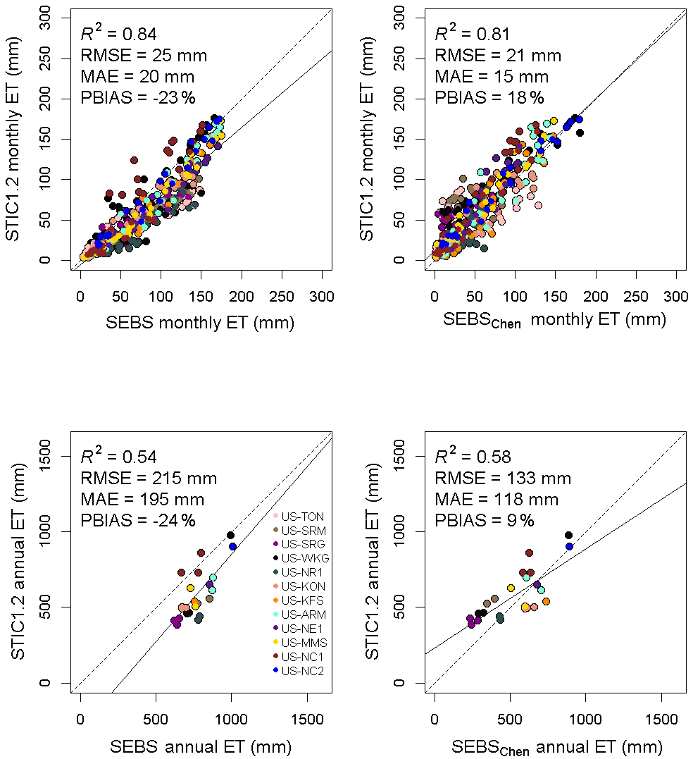
Figure 14Scatter plots of monthly and annual ET estimates from STIC1.2 against those from SEBS and a recently developed global SEBS products (Chen et al., 2013) with improved kB−1 characterization. Monthly SEBS and STIC1.2 ET estimates were produced using an aggregation of 8-day average EF multiplied by monthly total net radiation (similar to Eq. 17).
The wide use of the global MOD16 ET product for calculating regional water and energy balances should be evaluated on a case-by-case basis as one could come to different conclusions using ET outputs from the other two models considered in this study. A significant underestimation of actual ET by the MOD16 ET products, particularly in arid and semiarid conditions has already been reported (Hu et al., 2015; Ramoelo et al., 2014; Feng et al., 2012). Conversely, others have reported better performance of MOD16 ET products in humid climates (Hu et al., 2015) and forest ecosystems (Kim et al., 2012), consistent with the performance of the model in the two flux sites in North Carolina in our study (Table S1). Underestimation of ET by the MOD16 ET products in croplands has also been reported (Velpuri et al., 2013; Kim et al., 2012; Yang et al., 2015; Biggs et al., 2016), though not to the same extent as found in this study. Yang et al. (2015) highlighted four key uncertainties associated with the MOD16 algorithm (Mu et al., 2011), which could explain the relatively poor performance of MOD16 in this study. First, the dependency of the MOD16 algorithm on meteorological forcing (and not the TR) to account for the soil moisture restriction on evaporation and transpiration results in a slow response of variations in energy and heat fluxes (Long and Singh, 2010). Second, underestimation of transpiration in MOD16 could occur due to overestimation of environmental stresses on canopy conductance that is expressed as the potential canopy conductance multiplied by two empirical scaling factors that represent influences from TA and DA (Yang et al., 2013) Third, the empirical nature of the soil moisture constraint function (Fisher et al., 2008) based on the complementary hypothesis (Bouchet, 1963) using DA and RH leads to large uncertainties in evaporation from the unsaturated soil. Finally, the coarse resolution meteorological data (1∘ × 1.25∘) used in MOD16 may not be well representative of surfaces with high moisture variability. Additionally, the empirical scaling functions used for constraining the conductances and the spatial-scale mismatch between MODIS and flux towers could also introduce additional uncertainties in MOD16 ET. Similarly, our results suggest that caution should be taken when applying SEBS under the extreme dry condition, and also for grasslands, savannas, and deciduous broadleaf forests. The overestimation of grassland ET from SEBS is consistent with a recent study (Bhattarai et al., 2016), which could be attributed to the uncertain characterization of zOH (Gokmen et al., 2012). However, the performance of SEBS was relatively better under wet conditions, and in homogeneous croplands and evergreen needleleaf forests (Fig. 5, Table S1).
Apart from the simple parameterization of zOM and canopy heights using NDVI, another source of uncertainty in the implementation of STIC1.2 and SEBS at the 8-day timescale (using MOD11A2) could be the use of average 8-day daily time meteorological inputs that may not well correspond with LST observation days within each MODIS 8-day cycle. We found all 8-day daytime-averaged meteorological variables (those used in STIC1.2 and SEBS) except wind speed to be good representative of instantaneous measurements within the 8-day period (Table S2). This could be a source of additional uncertainty in SEBS since it uses wind speed to parameterize the aerodynamic conductance using MOST. Model implementation at an instantaneous timescale (i.e., MODIS overpass time and using daily MODIS products including MOD11A1 datasets) showed that the performance of STIC1.2 (R2 = 0.61, PBIAS = −5 %) was similar to its performance at the 8-day timescale. However, for SEBS (R2 = 0.53) the performance was marginally better with a PBIAS of 17 % (Table S3). In addition to the wind speed, the slight overestimation of 8-day average ϕ (PBIAS = 9 %), and variations in TR, TA, TR − TA, and other meteorological variables during days within the corresponding 8-day period could have added positive biases to SEBS (increase from 17 to 28 %), when evaluated at the 8-day timescale. Conversely, the overestimation in ϕ could have slightly reduced STIC1.2 biases (increase from −5 to −3 %). SEBS is sensitive to the meteorological input, especially the temperature gradient, and its performance is expected to degrade with the use of gridded forcing data (Ershadi et al., 2013; McCabe et al., 2016; van der Kwast et al., 2009; Vinukollu et al., 2011). Lewis et al. (2014) suggested that wind speed from NLDAS-2 may not be as reliable as other meteorological variables (TA and RH) in the western US. Overall, the application of STIC1.2 and SEBS at the instantaneous timescale showed similar predictive capacity and potential model strengths and weaknesses. STIC1.2 appears to be consistent through time, which could be due to the analytical nature, and STIC1.2 does not rely on wind speed to solve for gA and gC. Results also suggest that biases from SEBS could be within 20% if uncertainties associated with meteorological and radiative forcing are reduced.
This paper establishes the first ever regional-scale implementation of a simplified thermal remote-sensing-based model, Surface Temperature Initiated Closure (STIC1.2) for spatially explicit ET mapping, which is independent of any empirical parameterization of aerodynamic/surface conductances and aerodynamic temperature. By combining MODIS land surface temperature, surface reflectances, and gridded weather data, we demonstrate the promise of STIC1.2 to generate regional ET at 1 km × 1 km spatial resolution in the conterminous US. Independent validation of STIC1.2 using observed flux data from dry, wet, and normal precipitation years at 13 core AmeriFlux sites covering a wide range of climatic, biome, and aridity gradients in the US led us to the following conclusions.
- i.
Overall, STIC1.2 explained significant variability in the observed 8-day cumulative ET with a root mean square error (RMSE) of less than 1 mm day−1 and was robust throughout dry, wet, and normal years. Biome-wise evaluation of STIC1.2 suggests the smallest errors in forest ecosystems, followed by grassland, cropland, and woody savannas. Underestimation of ET in croplands is mainly attributed to the spatial-scale mismatch between a MODIS pixel and the flux tower footprint in croplands, and an overestimation of ET in woody savannas is mainly attributed to the large uncertainties in the MODIS LST product in savannas, and SEB closure correction of EC ET observations.
- ii.
STIC1.2 performed substantially better or comparable to SEBS and MOD16 in a broad spectrum of aridity, biome, and dry–wet extremes. Model evaluation in different aridity conditions suggests that all three models performed better under sub-humid and humid conditions as compared to arid or semi-arid conditions.
- iii.
The principal difference between STIC1.2 and SEBS ET appears to be associated with the differences in aerodynamic conductance estimation between the two models. Empirical characterization of z0M and kB−1 in SEBS are found to be the major factors creating uncertainties in aerodynamic conductance and ET estimations in SEBS, which is eventually responsible for large ET differences between the two models. Similarly, the differences in aerodynamic and surface conductance estimation between STIC1.2 and MOD16 could also be responsible for ET differences between the two models.
- iv.
STIC1.2 is highly sensitive to uncertainties in TR and hence accurate TR maps are needed for reliable ET estimates, which are currently missing in arid and semiarid ecosystems. However, with the improved emissivity corrected TR from the new MODIS LST product (MOD21; Hulley et al., 2014, 2016), an improved performance of STIC1.2 is expected in woody savannas. Alternatively, the use of time difference TR from MODIS Terra and Aqua can also help diminish STIC1.2 errors in woody savannas. Besides, gridded weather inputs (air temperature, RH, solar radiation), ideally at the resolution of TR, are required for STIC1.2 implementation and hence any errors associated with the weather inputs will create biased model outputs. These insights should provide guidance for future implementations of STIC1.2 in the US and other regions.
A1 Table of symbols and their description used in the study
| Symbol | Description |
|---|---|
| λ | Latent heat of vaporization of water (J kg−1 K−1) |
| H | Sensible heat flux (W m−2) |
| RN | Net radiation (W m−2) |
| RS | Shortwave radiation (W m−2) |
| Rld | Incoming longwave radiation (W m−2) |
| Rlu | Outgoing longwave radiation (W m−2) |
| G | Ground heat flux (W m−2) |
| ϕ | Available energy (W m−2) |
| ET | Evapotranspiration (evaporation + transpiration) as depth of water (mm) |
| λE | Latent heat flux (W m−2) |
| Ep | Potential evaporation as depth of water (mm) |
| gA | Aerodynamic conductance (m s−1) |
| gC | Canopy (or surface) conductance (m s−1) |
| rA | Aerodynamic resistance (s m−1) |
| rC | Canopy (or surface) resistance (s m−1) |
| M | Aggregated surface moisture availability (0–1) |
| TA | Air temperature (∘C) |
| TD | Dew point temperature of the air (∘C) |
| TR | Radiometric surface temperature (∘C) |
| TSD | Dew point temperature at the source/sink height (∘C) |
| T0 | Aerodynamic surface temperature (∘C) |
| RH | Relative humidity (%) |
| eA | Atmospheric vapor pressure (hPa) at the level of TA measurement |
| DA | Atmospheric vapor pressure deficit (hPa) at the level of TA measurement |
| eS | Vapor pressure at the surface (hPa) |
| Saturation vapor pressure at surface (hPa) | |
| Saturation vapor pressure at the source/sink height (hPa) | |
| e0 | Saturation vapor pressure at the source/sink height (hPa) |
| s | Slope of saturation vapor pressure vs. temperature curve (hPa K−1) |
| s1 | Slope of saturation vapor pressure and temperature between (TSD − TD) |
| vs. (e0 − eA), approximated at TD (hPa K−1) | |
| s2 | Slope of saturation vapor pressure and temperature between (TR − TD) |
| vs. ( − eA), estimated according to Mallick et al. (2015) (hPa K−1) | |
| γ | Psychrometric constant (hPa K−1) |
| ρA | Density of air (kg m−3) |
| cp | Specific heat of dry air (MJ kg−1 K−1) |
| Λ | Evaporative fraction |
| ΛR | Relative evaporation (–) |
| θ | Surface (0–5 cm) soil moisture (m3 m−3) |
| LAI | Leaf area index (m2 m−2) |
| NDVI | Normalized difference vegetation index (–) |
| β | Bowen ratio (–) |
| θv | Virtual potential temperature near the surface (K) |
| εo | Surface emissivity (–) |
| αo | Surface albedo (–) |
| u* | Friction velocity (m s−1) |
| Symbol | Description |
|---|---|
| RN24 | Daily net radiation (W m−2) |
| RN24,8-day | 8-day net radiation (W m−2) |
| kB−1 | Excess resistance to the heat transfer parameter (–) |
| λEwet | λE at wet limits (W m−2) |
| Hwet | H at wet limits (W m−2) |
| Hdry | H at dry limits (W m−2) |
| L | Monin–Obukhov length (m) |
| g | Acceleration due to gravity (9.8 m s−2) |
| d0 | Zero plane displacement height (m) |
| ΨH | Atmospheric stability correction for heat transport (–) |
| ΨM | Atmospheric stability correction for momentum transfer (–) |
| z0M | Roughness length for momentum transfer (m) |
| z0H | Roughness length for heat transfer (m) |
| z | Reference height (m) |
| zb | Blending height (m) |
| k | von Kármán constant (–) |
A2 Derivation of “state equations” in STIC1.2
After neglecting the horizontal advection and energy storage, the surface energy balance (SEB) equation is written as
While H is controlled by a single aerodynamic resistance (rA; or 1∕gA), λE is controlled by two resistances in series: the canopy (or surface) resistance (rC or 1∕gC) and the aerodynamic resistance to vapor transfer (rC + rA). For simplicity, it is implicitly assumed that the aerodynamic resistance of water vapor and heat are equal (Raupach, 1998), and both fluxes are transported from the same level from near-surface to the atmosphere. The sensible and latent heat flux can be expressed in the form of aerodynamic transfer equations (Boegh et al., 2002; Boegh and Soegaard, 2004) as follows:
where T0 and e0 are the air temperature and vapor pressure at the source/sink height and represent the vapor pressure and temperature of the quasi-laminar boundary layer in the immediate vicinity of the surface level. T0 can be obtained by extrapolating the logarithmic profile of TA down to z0H.
By combining Eqs. (A1)–(A3) and solving for gA, we get the following equation.
Combining the aerodynamic expressions of λE in Eq. (A3) and solving for gC, we can express gC as a function of gA and vapor pressure gradients.
In Eqs. (A4) and (A5), two more unknown variables (e0 and T0) are introduced resulting into two equations and four unknowns. Hence, two more equations are needed to close the system of equations. An expression for T0 is derived from the Bowen ratio (β; Bowen, 1926) and evaporative fraction (Λ; Shuttleworth et al., 1989) equation as
The expression for T0 introduces another new variable (Λ); therefore, one more equation that describes the dependence of Λ on the conductances (gA and gC) is needed to close the system of equations. In order to express Λ in terms of gA and gC, STIC1.2 adopts the advection-aridity (AA) hypothesis (Brutsaert and Stricker, 1979) with a modification introduced by Mallick et al. (2015). The AA hypothesis is based on a complementary connection between the potential evaporation (EP), sensible heat flux (H), and ET; and leads to an assumed link between gA and T0. However, the effects of surface moisture (or water stress) were not explicit in the AA equation and Mallick et al. (2015) implemented a moisture constraint in the original AA hypothesis while deriving a “state equation” of Λ (Eq. A8). A detailed derivation of the “state equation” for Λ is described in Mallick et al. (2014, 2015, 2016).
A3 Estimating e0, , M, and α in STIC1.2
In the early versions of STIC (Mallick et al., 2014, 2015), no distinction was made between the surface and source/sink height vapor pressures and hence was approximated as the saturation vapor pressure at TR. Then e0 was estimated from M with an assumption that the vapor pressure at the source/sink height scales between extreme wet–dry surface conditions. However, the level of and e0 should be consistent with the level of T0 from which the sensible heat flux is transferred (Lhomme and Montes, 2014). To use the PM equation predictively, it is imperative to consider the feedback between the surface layer evaporative fluxes and source/sink height mixing and coupling (McNaughton and Jarvis, 1984). Therefore, STIC1.2 uses physical expressions for estimating and e0 followed by estimating TSD and M as described below.
An estimate of is obtained by inverting the aerodynamic transfer equation of λE.
Following Shuttleworth and Wallace (1985; SW), the vapor pressure deficit (D0; = − e0) and e0 at the source/sink height are expressed as follows.
A physical equation of α is derived by expressing Λ as a function of the aerodynamic equations H and λE.
Combining Eqs. (A14) and (A8) (eliminating Λ), α can be expressed as
Following Venturini et al. (2008), and the theory of psychrometric slope of saturation vapor pressure vs. temperatures, M is expressed as the ratio of the dew point temperature difference between the source/sink height and air to the temperature difference between TR and dew point temperature of the air (TD).
where TSD is the dew point temperature at the source/sink height; s1 and s2 are the psychrometric slopes of the saturation vapor pressure and temperature between (TSD–TD) vs. (e0–eA) and (TR–TD) vs. (–eA) relationship (Venturini et al., 2008); and κ is the ratio between (–eA) and (–eA). Despite T0 driving the sensible heat flux, the comprehensive dry–wet signature of the underlying surface due to soil moisture variations is directly reflected in TR (Kustas and Anderson, 2009). Therefore, using TR in the denominator of Eq. (A16) tends to give a direct signature of the surface moisture availability (M).
In Eq. (A16), both s1 and TSD are unknowns, and an initial estimate of TSD is obtained using Eq. (6) of Venturini et al. (2008) where s1 was approximated in TD. From the initial estimates of TSD, an initial estimate of M is obtained as M = s1(TSD − TD)∕s2(TR − TD). However, since TSD also depends on λE, an iterative updating of TSD (and M) is carried out by expressing TSD as a function of λE as described below (also in Mallick et al., 2016). By decomposing the aerodynamic equation of λE, TSD can be expressed as follows.
An initial value of α is assigned as 1.26 and initial estimates of and e0 are obtained from TR and M as = 6.13753 and e0 = eA + − eA). Initial TSD and M were estimated from Eq. (6) of Venturini et al. (2008) and Eq. (A16), respectively. With the initial estimates of these variables, initial estimates of the conductances, T0, Λ, and λE are obtained. This process is then iterated by updating (using Eq. A9), D0 (using Eq. A10), e0 (using Eq. A11), TSD (using Eq. A18 with s1 estimated at TD), M (using Eq. A16), and α (using Eq. A15) with the initial estimates of gC, gA, and λE, and recomputing gC, gA, T0, Λ, and λE in the subsequent iterations with the previous estimates of , e0, TSD, M, and α until the convergence of λE is achieved. Stable values of λE, , e0, TSD, M, and α are obtained within ∼ 25 iterations.
All data used in this study are publicly available from different sources. Flux data from the AmeriFlux sites are available at http://ameriflux.lbl.gov/ (last access: 5 March 2017). MODIS (https://modis.gsfc.nasa.gov/data/, last access: 6 March 2017) and NLDAS-2 data (https://ldas.gsfc.nasa.gov/nldas/NLDAS2forcing.php, last access: 10 February 2017) are made freely available by NASA. PRISM data can be downloaded from http://prism.oregonstate.edu/ (last access: 9 March 2017), made available by the PRISM Climate Group at Oregon State University. MOD16 ET data, developed by the Numerical Terradynamic Simulation Group at the University of Montana, are available at http://files.ntsg.umt.edu/data/NTSG_Products/MOD16/ (last access: 15 March 2017). Daily GridMet data are available from the University of Idaho (http://www.climatologylab.org/gridmet.html, last access: 10 March 2017). Model codes used in this paper are available upon request to the corresponding author.
The supplement related to this article is available online at: https://doi.org/10.5194/hess-22-2311-2018-supplement.
The authors declare that they have no conflict of interest.
The study was party supported by the NASA new investigator program award (NNX16AI19G) and a NASA Land-Cover Land-Use Change Grant (NNX17AH97G) to Meha Jain. Kaniska Mallick was supported by the Luxembourg Institute of Science and Technology (LIST) through the project BIOTRANS (grant number 00001145) and CAOS-2 project grant (INTER/DFG/14/02) funded by FNR (Fonds National de la Recherche) – DFG (German Science Foundation). This project also contributes to HiWET consortium funded by the Belgian Science Policy (BELSPO) – FNR under the programme STEREOIII (INTER/STEREOIII/13/03/HiWET; CONTRACT NR SR/00/301).
Funding for AmeriFlux core site data was provided by the US Department of
Energy's Office of Science. The authors would like to thank all the principal
investigators: Russell Scott, USDA-ARS (US-Wkg, US-SRM, and US-SRG);
Asko Noormets, North Carolina State University (US-NC1 and US-NC2);
Sebastien Biraud, Lawrence Berkeley National Lab (US-ARM);
Dennis Baldocchi, University of California, Berkeley (US-Ton); Nathaniel A. Brunsell
(NAB), University of Kansas (US-KFS and US-Kon); Kim Novick,
Indiana University (US-MMS); Peter Blanken, University of Colorado
(US-NR1); Andy Suyker, University of Nebraska, Lincoln (US-Ne1); and
Bev Law, Oregon State University (US-Me2) for maintaining and providing
access to the flux data for free. Nathaniel A. Brunsell acknowledges funding for the US-Kon
site through the NSF Long Term Ecological Research grant to the Konza
Prairie (DEB-0823341), and for the US-Kon and US-KFS sites through AmeriFlux
core site funding from the US Department of Energy under a sub contract from
DE-AC02-05CH11231 and additional funding support through the USDA-AFRI
2014-67003-22070. The authors would also like to thank Bob Su and
Xuelong Chen from the University of Twente, the Netherlands for answering
queries related to the SEBS model. Special thanks to Julia Stuart
(undergraduate researcher) for helping out with the literature search. The
authors would like to acknowledge high-performance computing support from
Yellowstone (ark:/85065/d7wd3xhc) provided by NCAR's Computational and
Information Systems Laboratory, sponsored by the National Science
Foundation. Finally, the authors would also like to thank all the reviewers
for useful comments and suggestions to improve this manuscript.
Edited by: Bob Su
Reviewed by: three anonymous referees
Abatzoglou, J. T.: Development of gridded surface meteorological data for ecological applications and modelling, Int. J. Climatol., 33, 121–131, https://doi.org/10.1002/joc.3413, 2013.
Abouali, M., Timmermans, J., Castillo, J. E., and Su, B. Z.: A high performance GPU implementation of Surface Energy Balance System (SEBS) based on CUDA-C, Environ. Model. Softw., 41, 134–138, 2013.
Agam, N. and Berliner, P. R.: Dew formation and water vapor adsorption in semi-arid environments – A review, J. Arid Environm., 65, 572–590, https://doi.org/10.1016/j.jaridenv.2005.09.004, 2006.
Allen, R. G., Tasumi, M., and Trezza, R.: Satellite-based energy balance for mapping evapotranspiration with internalized calibration (METRIC) – Model, J. Irrig. Drain. Eng., 133, 380–394, https://doi.org/10.1061/(Asce)0733-9437(2007)133:4(380), 2007.
Allen, R. G., Irmak, A., Trezza, R., Hendrickx, J. M. H., Bastiaanssen, W., and Kjaersgaard, J.: Satellite-based ET estimation in agriculture using SEBAL and METRIC, Hydrol. Process., 25, 4011–4027, https://doi.org/10.1002/hyp.8408, 2011.
AmeriFlux Network: http://ameriflux.lbl.gov/, last access: 5 March 2017.
Anderson, M. C., Kustas, W. P., Norman, J. M., Hain, C. R., Mecikalski, J. R., Schultz, L., Gonzalez-Dugo, M. P., Cammalleri, C., d'Urso, G., Pimstein, A., and Gao, F.: Mapping daily evapotranspiration at field to continental scales using geostationary and polar orbiting satellite imagery, Hydrol. Earth Syst. Sci., 15, 223–239, https://doi.org/10.5194/hess-15-223-2011, 2011.
Anderson, M. C., Allen, R. G., Morse, A., and Kustas, W. P.: Use of Landsat thermal imagery in monitoring evapotranspiration and managing water resources, Remote Sens. Environ., 122, 50–65, https://doi.org/10.1016/j.rse.2011.08.025, 2012.
ASCE-EWRI: The ASCE standardized reference evapotranspiration equation, ASCE-EWRI Standardization of Reference Evapotranspiration Task Committe Report, 2005,
Baldocchi, D. D., and Wilson, K. B.: Modeling CO2 and water vapor exchange of a temperate broadleaved forest across hourly to decadal time scales, Ecol. Model., 142, 155–184, https://doi.org/10.1016/S0304-3800(01)00287-3, 2001.
Baldocchi, D. D., Xu, L., and Kiang, N.: How plant functional-type, weather, seasonal drought, and soil physical properties alter water and energy fluxes of an oak–grass savanna and an annual grassland, Agr. Forest Meteorol., 123, 13–39, https://doi.org/10.1016/j.agrformet.2003.11.006, 2004.
Bastiaanssen, W. G. M.: SEBAL-based sensible and latent heat fluxes in the irrigated Gediz Basin, Turkey, J. Hydrol., 229, 87–100, https://doi.org/10.1016/S0022-1694(99)00202-4, 2000.
Bell, D. M., Ward, E. J., Oishi, A. C., Oren, R., Flikkema, P. G., and Clark, J. S.: A state-space modeling approach to estimating canopy conductance and associated uncertainties from sap flux density data, Tree Physiol., 35, 792–802, https://doi.org/10.1093/treephys/tpv041, 2015.
Bhattarai, N., Shaw, S. B., Quackenbush, L. J., Im, J., and Niraula, R.: Evaluating five remote sensing based single-source surface energy balance models for estimating daily evapotranspiration in a humid subtropical climate, Int. J. Appl. Earth Obs., 49, 75–86, https://doi.org/10.1016/j.jag.2016.01.010, 2016.
Biggs, T. W., Marshall, M., and Messina, A.: Mapping daily and seasonal evapotranspiration from irrigated crops using global climate grids and satellite imagery: Automation and methods comparison, Water Resour. Res., 52, 7311–7326, https://doi.org/10.1002/2016WR019107, 2016.
Bisht, G., Venturini, V., Islam, S., and Jiang, L.: Estimation of the net radiation using MODIS (Moderate Resolution Imaging Spectroradiometer) data for clear sky days, Remote Sens. Environ., 97, 52–67, https://doi.org/10.1016/j.rse.2005.03.014, 2005.
Blonquist, J. M., Norman, J. M., and Bugbee, B.: Automated measurement of canopy stomatal conductance based on infrared temperature, Agr. Forest Meteorol., 149, 1931–1945, https://doi.org/10.1016/j.agrformet.2009.06.021, 2009.
Boegh, E. and Soegaard, H.: Remote sensing based estimation of evapotranspiration rates, Int. J. Remote Sens., 25, 2535–2551, https://doi.org/10.1080/01431160310001647975, 2004.
Boegh, E., Soegaard, H., and Thomsen, A.: Evaluating evapotranspiration rates and surface conditions using Landsat TM to estimate atmospheric resistance and surface resistance, Remote Sens. Environ., 79, 329–343, https://doi.org/10.1016/S0034-4257(01)00283-8, 2002.
Bouchet, R.: Evapotranspiration reelle, evapotranspiration potentielle, et production agricole, Annales Agronomiques, 14, 743–824, 1963.
Boulet, G., Olioso, A., Ceschia, E., Marloie, O., Coudert, B., Rivalland, V., Chirouze, J., and Chehbouni, G.: An empirical expression to relate aerodynamic and surface temperatures for use within single-source energy balance models, Agr. Forest Meteorol., 161, 148–155, https://doi.org/10.1016/j.agrformet.2012.03.008, 2012.
Bowen, I. S.: The ratio of heat losses by conduction and by evaporation from any water surface, Phys. Rev., 27, 779, 1926.
Brutsaert, W.: Hydrology: an introduction, Cambridge University Press, Cambridge, 2005.
Brutsaert, W. and Stricker, H.: An advection-aridity approach to estimate actual regional evapotranspiration, Water Resour. Res., 15, 443–450, https://doi.org/10.1029/WR015i002p00443, 1979.
Brutsaert, W. and Sugita, M.: Application of self-preservation in the diurnal evolution of the surface energy budget to determine daily evaporation, J. Geophys. Res.-Atmos., 97, 18377–18382, https://doi.org/10.1029/92JD00255, 1992.
Chávez, J., Neale, C. M. U., Hipps, L. E., Prueger, J. H., and Kustas, W. P.: Comparing Aircraft-Based Remotely Sensed Energy Balance Fluxes with Eddy Covariance Tower Data Using Heat Flux Source Area Functions, J. Hydrometeorol., 6, 923–940, https://doi.org/10.1175/jhm467.1, 2005.
Chávez, J., Howell, T., Gowda, P., Copeland, K., and Prueger, J.: Surface aerodynamic temperature modeling over rainfed cotton, T. ASABE, 53, 759–767, 2010.
Chen, X., Su, Z., Ma, Y., Yang, K., Wen, J., and Zhang, Y.: An Improvement of Roughness Height Parameterization of the Surface Energy Balance System (SEBS) over the Tibetan Plateau, J. Appl. Meteorol. Clim., 52, 607–622, https://doi.org/10.1175/jamc-d-12-056.1, 2013.
Chen, X., Su, Z., Ma, Y., Liu, S., Yu, Q., and Xu, Z.: Development of a 10-year (2001–2010) 0.1∘ data set of land-surface energy balance for mainland China, Atmos. Chem. Phys., 14, 13097–13117, https://doi.org/10.5194/acp-14-13097-2014, 2014.
Colaizzi, P. D., Evett, S. R., Howell, T. A., and Tolk, J. A.: Comparison of aerodynamic and radiometric surface temperature using precision weighing lysimeters, in: Optical Science and Technology, the SPIE 49th Annual Meeting, 2–6 August 2004. Denver, Colorado, 215–229, 2004.
Crago, R. and Brutsaert, W.: Daytime evaporation and the self-preservation of the evaporative fraction and the Bowen ratio, J. Hydrol., 178, 241–255, https://doi.org/10.1016/0022-1694(95)02803-X, 1996.
Domec, J.-C., King, J. S., Ward, E., Christopher Oishi, A., Palmroth, S., Radecki, A., Bell, D. M., Miao, G., Gavazzi, M., Johnson, D. M., McNulty, S. G., Sun, G., and Noormets, A.: Conversion of natural forests to managed forest plantations decreases tree resistance to prolonged droughts, Forest Ecol. Manage., 355, 58–71, https://doi.org/10.1016/j.foreco.2015.04.012, 2015.
Ershadi, A., McCabe, M. F., Evans, J. P., Mariethoz, G., and Kavetski, D.: A Bayesian analysis of sensible heat flux estimation: Quantifying uncertainty in meteorological forcing to improve model prediction, Water Resour. Res., 49, 2343–2358, 2013.
FAO – Food and Agriculture Organization of the United Nations: FAO GEONETWORK, Aridity index (GeoLayer), http://data.fao.org/ref/f8cf2780-88fd-11da-a88f-000d939bc5d8.html?version=1.0 (last access: 9 April 2018), 2015.
Feng, X. M., Sun, G., Fu, B. J., Su, C. H., Liu, Y., and Lamparski, H.: Regional effects of vegetation restoration on water yield across the Loess Plateau, China, Hydrol. Earth Syst. Sci., 16, 2617–2628, https://doi.org/10.5194/hess-16-2617-2012, 2012.
Finnigan, J. J., Shaw, R. H., and Patton, E. G.: Turbulence structure above a vegetation canopy, J. Fluid Mech., 637, 387–424, https://doi.org/10.1017/S0022112009990589, 2009.
Fischer, M. L., Billesbach, D. P., Berry, J. A., Riley, W. J., and Torn, M. S.: Spatiotemporal Variations In Growing Season Exchanges Of CO2, H2O, And Sensible Heat In Agricultural Fields Of The Southern Great Plains, Earth Interact., 11, 1–21, 2007.
Fisher, J. B., Tu, K. P., and Baldocchi, D. D.: Global estimates of the land–atmosphere water flux based on monthly AVHRR and ISLSCP-II data, validated at 16 FLUXNET sites, Remote Sens. Environ., 112, 901–919, https://doi.org/10.1016/j.rse.2007.06.025, 2008.
Foken, T.: 50 Years of the Monin–Obukhov Similarity Theory, Bound.-Lay. Meteorol., 119, 431–447, https://doi.org/10.1007/s10546-006-9048-6, 2006.
Friedl, M. A., Sulla-Menashe, D., Tan, B., Schneider, A., Ramankutty, N., Sibley, A., and Huang, X.: MODIS Collection 5 global land cover: Algorithm refinements and characterization of new datasets, Remote Sens. Environ., 114, 168–182, https://doi.org/10.1016/j.rse.2009.08.016, 2010.
Garratt, J. R.: Flux profile relations above tall vegetation, Q. J. Roy. Meteorol. Soc., 104, 199–211, https://doi.org/10.1002/qj.49710443915, 1978.
Gokmen, M., Vekerdy, Z., Verhoef, A., Verhoef, W., Batelaan, O., and van der Tol, C.: Integration of soil moisture in SEBS for improving evapotranspiration estimation under water stress conditions, Remote Sens. Environ., 121, 261–274, https://doi.org/10.1016/j.rse.2012.02.003, 2012.
GRIDMET: http://www.climatologylab.org/gridmet.html, last access: 10 March 2017.
Harman, I. N. and Finnigan, J. J.: A simple unified theory for flow in the canopy and roughness sublayer, Bound.-Lay. Meteorol., 123, 339–363, https://doi.org/10.1007/s10546-006-9145-6, 2007.
Holwerda, F., Bruijnzeel, L., Scatena, F., Vugts, H., and Meesters, A.: Wet canopy evaporation from a Puerto Rican lower montane rain forest: The importance of realistically estimated aerodynamic conductance, J. Hydrol., 414, 1–15, 2012.
Hu, G., Jia, L., and Menenti, M.: Comparison of MOD16 and LSA-SAF MSG evapotranspiration products over Europe for 2011, Remote Sens. Environ., 156, 510–526, https://doi.org/10.1016/j.rse.2014.10.017, 2015.
Hulley, G. C., Hughes, C. G., and Hook, S. J.: Quantifying uncertainties in land surface temperature and emissivity retrievals from ASTER and MODIS thermal infrared data, J. Geophys. Res.-Atmos., 117, D23113, https://doi.org/10.1029/2012JD018506, 2012.
Hulley, G. C., Veraverbeke, S., and Hook, S.: Thermal-based techniques for land cover change detection using a new dynamic MODIS multispectral emissivity product (MOD21), Remote Sens. Environ., 140, 755–765, https://doi.org/10.1016/j.rse.2013.10.014, 2014.
Hulley, G. C., Malakar, N., Hughes, T., Islam, T., and Hook, S.: Moderate resolution imaging spectroradiometer (MODIS) MOD21 land surface temperature and emissivity algorithm theoretical basis document, Jet Propulsion Laboratory, National Aeronautics and Space Administration, Pasadena, CA, 2016.
Jin, M. and Liang, S.: An Improved Land Surface Emissivity Parameter for Land Surface Models Using Global Remote Sensing Observations, J. Climate, 19, 2867–2881, https://doi.org/10.1175/jcli3720.1, 2006.
Kim, H. W., Hwang, K., Mu, Q., Lee, S. O., and Choi, M.: Validation of MODIS 16 global terrestrial evapotranspiration products in various climates and land cover types in Asia, KSCE J. Civ. Eng., 16, 229–238, https://doi.org/10.1007/s12205-012-0006-1, 2012.
Kustas, W. P. and Anderson, M.: Advances in thermal infrared remote sensing for land surface modeling, Agr. Forest Meteorol., 149, 2071–2081, https://doi.org/10.1016/j.agrformet.2009.05.016, 2009.
Kustas, W. P. and Norman, J.: Use of remote sensing for evapotranspiration monitoring over land surfaces, Hydrolog. Sci. J., 41, 495–516, 1996.
Kustas, W. P. and Norman, J. M.: A two-source approach for estimating turbulent fluxes using multiple angle thermal infrared observations, Water Resour. Res., 33, 1495–1508, https://doi.org/10.1029/97WR00704, 1997.
Kustas, W. P., Nieto, H., Morillas, L., Anderson, M. C., Alfieri, J. G., Hipps, L. E., Villagarcía, L., Domingo, F., and Garcia, M.: Revisiting the paper “Using radiometric surface temperature for surface energy flux estimation in Mediterranean drylands from a two-source perspective”, Remote Sens. Environ., 184, 645–653, https://doi.org/10.1016/j.rse.2016.07.024, 2016.
Lewis, C. S., Geli, H. M. E., and Neale, C. M. U.: Comparison of the NLDAS Weather Forcing Model to Agrometeorological Measurements in the western United States, J. Hydrol., 510, 385–392, https://doi.org/10.1016/j.jhydrol.2013.12.040, 2014.
Lhomme, J. P. and Montes, C.: Generalized combination equations for canopy evaporation under dry and wet conditions, Hydrol. Earth Syst. Sci., 18, 1137–1149, https://doi.org/10.5194/hess-18-1137-2014, 2014.
Liaw, A. and Wiener, M.: Classification and regression by randomForest, R News, 2, 18–22, 2002.
Liu, S., Lu, L., Mao, D., and Jia, L.: Evaluating parameterizations of aerodynamic resistance to heat transfer using field measurements, Hydrol. Earth Syst. Sci., 11, 769–783, https://doi.org/10.5194/hess-11-769-2007, 2007.
Logan, K. E. and Brunsell, N. A.: Influence of drought on growing season carbon and water cycling with changing land cover, Agr. Forest Meteorol., 213, 217–225, https://doi.org/10.1016/j.agrformet.2015.07.002, 2015.
Long, D. and Singh, V. P.: Integration of the GG model with SEBAL to produce time series of evapotranspiration of high spatial resolution at watershed scales, J. Geophys. Res.-Atmos., 115, D21128, https://doi.org/10.1029/2010JD014092, 2010.
Mallick, K., Jarvis, A. J., Boegh, E., Fisher, J. B., Drewry, D. T., Tu, K. P., Hook, S. J., Hulley, G., Ardo, J., Beringer, J., Arain, A., and Niyogi, D.: A Surface Temperature Initiated Closure (STIC) for surface energy balance fluxes, Remote Sens. Environ., 141, 243–261, https://doi.org/10.1016/j.rse.2013.10.022, 2014.
Mallick, K., Boegh, E., Trebs, I., Alfieri, J. G., Kustas, W. P., Prueger, J. H., Niyogi, D., Das, N., Drewry, D. T., Hoffmann, L., and Jarvis, A. J.: Reintroducing radiometric surface temperature into the Penman–Monteith formulation, Water Resour. Res., 51, 6214–6243, https://doi.org/10.1002/2014wr016106, 2015.
Mallick, K., Trebs, I., Boegh, E., Giustarini, L., Schlerf, M., Drewry, D. T., Hoffmann, L., von Randow, C., Kruijt, B., Araùjo, A., Saleska, S., Ehleringer, J. R., Domingues, T. F., Ometto, J. P. H. B., Nobre, A. D., de Moraes, O. L. L., Hayek, M., Munger, J. W., and Wofsy, S. C.: Canopy-scale biophysical controls of transpiration and evaporation in the Amazon Basin, Hydrol. Earth Syst. Sci., 20, 4237–4264, https://doi.org/10.5194/hess-20-4237-2016, 2016.
Mallick, K., Toivonen, E., Trebs, I., Boegh, E., Cleverly, J., Eamus, D., Koivusalo, H., Dewry, D., Arndt, S. K., Griebel, A., Beringer, J., and Garcia, M.: Bridging thermal infrared sensing and physically-based evapotranspiration modeling: from theoretical implementation to validation across an aridity gradient in Australian ecosystems, Water Resour. Res., in press, 2018.
Matheny, A. M., Bohrer, G., Stoy, P. C., Baker, I. T., Black, A. T., Desai, A. R., Dietze, M. C., Gough, C. M., Ivanov, V. Y., Jassal, R. S., Novick, K. A., Schafer, K. V. R., and Verbeeck, H.: Characterizing the diurnal patterns of errors in the prediction of evapotranspiration by several land-surface models: An NACP analysis, J. Geophys. Res.-Biogeo., 119, 1458–1473, https://doi.org/10.1002/2014jg002623, 2014.
McCabe, M. F., Ershadi, A., Jimenez, C., Miralles, D. G., Michel, D., and Wood, E. F.: The GEWEX LandFlux project: evaluation of model evaporation using tower-based and globally gridded forcing data, Geosci. Model Dev., 9, 283–305, https://doi.org/10.5194/gmd-9-283-2016, 2016.
McHugh, T. A., Morrissey, E. M., Reed, S. C., Hungate, B. A., and Schwartz, E.: Water from air: an overlooked source of moisture in arid and semiarid regions, Scient. Rep., 5, 13767, https://doi.org/10.1038/srep13767, 2015.
McIntosh, D. H. and Thom, A. S.: Essentials of meteorology, Wykeham, London, 1978.
McNaughton, K. G. and Jarvis, P. G.: Using the Penman-Monteith equation predictively, Agr. Water Manage., 8, 263–278, https://doi.org/10.1016/0378-3774(84)90057-X, 1984.
Mitchell, K. E., Lohmann, D., Houser, P. R., Wood, E. F., Schaake, J. C., Robock, A., Cosgrove, B. A., Sheffield, J., Duan, Q., Luo, L., Higgins, R. W., Pinker, R. T., Tarpley, J. D., Lettenmaier, D. P., Marshall, C. H., Entin, J. K., Pan, M., Shi, W., Koren, V., Meng, J., Ramsay, B. H., and Bailey, A. A.: The multi-institution North American Land Data Assimilation System (NLDAS): Utilizing multiple GCIP products and partners in a continental distributed hydrological modeling system, J. Geophys. Res.-Atmos., 109, D07S90, https://doi.org/10.1029/2003JD003823, 2004.
MOD16: Evapotranspiration products, http://files.ntsg.umt.edu/data/NTSG_Products/MOD16/, last access: 15 March 2017.
MODIS – Moderate Resolution Imaging Spectroradiometer: Data Products, https://modis.gsfc.nasa.gov/data/dataprod/, last access: 6 March 2017.
Moffett, K. B. and Gorelick, S. M.: A method to calculate heterogeneous evapotranspiration using submeter thermal infrared imagery coupled to a stomatal resistance submodel, Water Resour. Res., 48, W01545, https://doi.org/10.1029/2011WR010407, 2012.
Monson, R. K., Sparks, J. P., Rosenstiel, T. N., Scott-Denton, L. E., Huxman, T. E., Harley, P. C., Turnipseed, A. A., Burns, S. P., Backlund, B., and Hu, J.: Climatic influences on net ecosystem CO2 exchange during the transition from wintertime carbon source to springtime carbon sink in a high-elevation, subalpine forest, Oecologia, 146, 130–147, https://doi.org/10.1007/s00442-005-0169-2, 2005.
Monteith, J. L.: Evaporation and environment, Symp. Soc. Exp. Biol., 19, 4, 1965.
Monteith, J. L.: Evaporation and surface temperature, Q. J. Roy. Meteorol. Soc., 107, 1–27, https://doi.org/10.1002/qj.49710745102, 1981.
Mu, Q., Zhao, M., and Running, S. W.: Improvements to a MODIS global terrestrial evapotranspiration algorithm, Remote Sens. Environ., 115, 1781–1800, https://doi.org/10.1016/j.rse.2011.02.019, 2011.
Mu, Q., Heinsch, F. A., Zhao, M., and Running, S. W.: Development of a global evapotranspiration algorithm based on MODIS and global meteorology data, Remote Sens. Environ., 111, 519–536, https://doi.org/10.1016/j.rse.2007.04.015, 2007.
Myneni, R. B., Hoffman, S., Knyazikhin, Y., Privette, J. L., Glassy, J., Tian, Y., Wang, Y., Song, X., Zhang, Y., Smith, G. R., Lotsch, A., Friedl, M., Morisette, J. T., Votava, P., Nemani, R. R., and Running, S. W.: Global products of vegetation leaf area and fraction absorbed PAR from year one of MODIS data, Remote Sens. Environ., 83, 214–231, https://doi.org/10.1016/S0034-4257(02)00074-3, 2002.
NLDAS-2 – North American Land Data Assimilation System: Forcing Dataset, https://ldas.gsfc.nasa.gov/nldas/NLDAS2forcing.php, last access: 10 February 2017.
Norman, J. M., Kustas, W. P., and Humes, K. S.: Source approach for estimating soil and vegetation energy fluxes in observations of directional radiometric surface temperature, Agr. Forest Meteorol., 77, 263–293, https://doi.org/10.1016/0168-1923(95)02265-Y, 1995.
Numata, I., Khand, K., Kjaersgaard, J., Cochrane, M. A., and Silva, S. S.: Evaluation of Landsat-Based METRIC Modeling to Provide High-Spatial Resolution Evapotranspiration Estimates for Amazonian Forests, Remote Sensing, 9, 46, 2017.
Paul, G., Gowda, P. H., Vara Prasad, P. V., Howell, T. A., Aiken, R. M., and Neale, C. M. U.: Investigating the influence of roughness length for heat transport (zoh) on the performance of SEBAL in semi-arid irrigated and dryland agricultural systems, J. Hydrol., 509, 231–244, https://doi.org/10.1016/j.jhydrol.2013.11.040, 2014.
Philip, R. and Novick, K.: AmeriFlux US-MMS Morgan Monroe State Forest, AmeriFlux, Indiana University, Indianapolis, Indiana, 2016.
Priestley, C. and Taylor, R.: On the assessment of surface heat flux and evaporation using large-scale parameters, Mon. Weather Rev., 100, 81–92, https://doi.org/10.1175/1520-0493(1972)100<0081:otaosh>2.3.co;2, 1972.
PRISM: Parameter elevation Regression on Independent Slopes Model: Climate Data, http://prism.oregonstate.edu, last access: 9 March 2017.
Ramoelo, A., Majozi, N., Mathieu, R., Jovanovic, N., Nickless, A., and Dzikiti, S.: Validation of Global Evapotranspiration Product (MOD16) using Flux Tower Data in the African Savanna, South Africa, Remote Sensing, 6, 7406–7423, 2014.
Raupach, M. R.: Influences of local feedbacks on land–air exchanges of energy and carbon, Global Change Biol., 4, 477–494, https://doi.org/10.1046/j.1365-2486.1998.t01-1-00155.x, 1998.
Scott, R. L., Biederman, J. A., Hamerlynck, E. P., and Barron-Gafford, G. A.: The carbon balance pivot point of southwestern U.S. semiarid ecosystems: Insights from the 21st century drought, J. Geophys. Res.-Biogeo., 120, 2612–2624, https://doi.org/10.1002/2015JG003181, 2015.
Shuttleworth, W. J. and Wallace, J. S.: Evaporation from sparse crops-an energy combination theory, Q. J. Roy. Meteorol. Soc., 111, 839–855, https://doi.org/10.1002/qj.49711146910, 1985.
Shuttleworth, W. J., Gurney, R., Hsu, A., and Ormsby, J.: FIFE: the variation in energy partition at surface flux sites, IAHS Publ., Baltimore, Maryland, 67–74, 1989.
Simpson, I. J., Thurtell, G. W., Neumann, H. H., Den Hartog, G., and Edwards, G. C.: The Validity of Similarity Theory in the Roughness Sublayer Above Forests, Bound.-Lay. Meteorol., 87, 69–99, https://doi.org/10.1023/a:1000809902980, 1998.
Stoy, P. C., Mauder, M., Foken, T., Marcolla, B., Boegh, E., Ibrom, A., Arain, M. A., Arneth, A., Aurela, M., Bernhofer, C., Cescatti, A., Dellwik, E., Duce, P., Gianelle, D., van Gorsel, E., Kiely, G., Knohl, A., Margolis, H., McCaughey, H., Merbold, L., Montagnani, L., Papale, D., Reichstein, M., Saunders, M., Serrano-Ortiz, P., Sottocornola, M., Spano, D., Vaccari, F., and Varlagin, A.: A data-driven analysis of energy balance closure across FLUXNET research sites: The role of landscape scale heterogeneity, Agr. Forest Meteorol., 171, 137–152, https://doi.org/10.1016/j.agrformet.2012.11.004, 2013.
Su, Z.: The Surface Energy Balance System (SEBS) for estimation of turbulent heat fluxes, Hydrol. Earth Syst. Sci., 6, 85–100, https://doi.org/10.5194/hess-6-85-2002, 2002.
Su, Z., Schmugge, T., Kustas, W. P., and Massman, W. J.: An evaluation of two models for estimation of the roughness height for heat transfer between the land surface and the atmosphere, J. Appl. Meteorol., 40, 1933–1951, 2001.
Sun, G., Noormets, A., Gavazzi, M. J., McNulty, S. G., Chen, J., Domec, J. C., King, J. S., Amatya, D. M., and Skaggs, R. W.: Energy and water balance of two contrasting loblolly pine plantations on the lower coastal plain of North Carolina, USA, Forest Ecol. Manage., 259, 1299–1310, https://doi.org/10.1016/j.foreco.2009.09.016, 2010.
Suyker, A.: AmeriFlux US-Ne1 Mead-irrigated continuous maize site, AmeriFlux, University of Nebraska-Lincoln, Mead, Nebraska, 2016.
Thomas, C. K., Law, B. E., Irvine, J., Martin, J. G., Pettijohn, J. C., and Davis, K. J.: Seasonal hydrology explains interannual and seasonal variation in carbon and water exchange in a semiarid mature ponderosa pine forest in central Oregon, J. Geophys. Res.-Biogeo., 114, G04006, https://doi.org/10.1029/2009JG001010, 2009.
Timmermans, J., Su, Z., van der Tol, C., Verhoef, A., and Verhoef, W.: Quantifying the uncertainty in estimates of surface–atmosphere fluxes through joint evaluation of the SEBS and SCOPE models, Hydrol. Earth Syst. Sci., 17, 1561–1573, https://doi.org/10.5194/hess-17-1561-2013, 2013.
Troufleau, D., Lhomme, J. P., Monteny, B., and Vidal, A.: Sensible heat flux and radiometric surface temperature over sparse Sahelian vegetation. I. An experimental analysis of the kB-1 parameter, J. Hydrol., 188, 815–838, https://doi.org/10.1016/S0022-1694(96)03172-1, 1997.
Tucker, C. J.: Red and photographic infrared linear combinations for monitoring vegetation, Remote Sens. Environ., 8, 127–150, 1979.
Twine, T. E., Kustas, W. P., Norman, J. M., Cook, D. R., Houser, P. R., Meyers, T. P., Prueger, J. H., Starks, P. J., and Wesely, M. L.: Correcting eddy-covariance flux underestimates over a grassland, Agr. Forest Meteorol., 103, 279–300, https://doi.org/10.1016/S0168-1923(00)00123-4, 2000.
van der Kwast, J., Timmermans, W., Gieske, A., Su, Z., Olioso, A., Jia, L., Elbers, J., Karssenberg, D., and de Jong, S.: Evaluation of the Surface Energy Balance System (SEBS) applied to ASTER imagery with flux-measurements at the SPARC 2004 site (Barrax, Spain), Hydrol. Earth Syst. Sci., 13, 1337–1347, https://doi.org/10.5194/hess-13-1337-2009, 2009.
van Dijk, A. I. J. M., Gash, J. H., van Gorsel, E., Blanken, P. D., Cescatti, A., Emmel, C., Gielen, B., Harman, I. N., Kiely, G., and Merbold, L.: Rainfall interception and the coupled surface water and energy balance, Agr. Forest Meteorol., 214, 402–415, 2015a.
van Dijk, A. I. J. M., Gash, J. H., van Gorsel, E., Blanken, P. D., Cescatti, A., Emmel, C., Gielen, B., Harman, I. N., Kiely, G., Merbold, L., Montagnani, L., Moors, E., Sottocornola, M., Varlagin, A., Williams, C. A., and Wohlfahrt, G.: Rainfall interception and the coupled surface water and energy balance, Agr. Forest Meteorol., 214–215, 402–415, https://doi.org/10.1016/j.agrformet.2015.09.006, 2015b.
Velpuri, N. M., Senay, G. B., Singh, R. K., Bohms, S., and Verdin, J. P.: A comprehensive evaluation of two MODIS evapotranspiration products over the conterminous United States: Using point and gridded FLUXNET and water balance ET, Remote Sens. Environ., 139, 35–49, https://doi.org/10.1016/j.rse.2013.07.013, 2013.
Venturini, V., Islam, S., and Rodriguez, L.: Estimation of evaporative fraction and evapotranspiration from MODIS products using a complementary based model, Remote Sens. Environ., 112, 132–141, https://doi.org/10.1016/j.rse.2007.04.014, 2008.
Verhoef, A., Bruin, H. A. R. D., and Hurk, B. J. J. M. V. D.: Some Practical Notes on the Parameter kB-1 for Sparse Vegetation, J. Appl. Meteorol., 36, 560–572, https://doi.org/10.1175/1520-0450(1997)036<0560:spnotp>2.0.co;2, 1997a.
Verhoef, A., McNaughton, K. G., and Jacobs, A. F. G.: A parameterization of momentum roughness length and displacement height for a wide range of canopy densities, Hydrol. Earth Syst. Sci., 1, 81–91, https://doi.org/10.5194/hess-1-81-1997, 1997b.
Vermote, E.: MOD09A1MODIS/Terra Surface Reflectance 8-Day L3 Global 500 m SIN Grid V006, NASA EOSDIS Land Processes DAAC, NASA, Greenbelt, Maryland, 2015.
Vinukollu, R. K., Wood, E. F., Ferguson, C. R., and Fisher, J. B.: Global estimates of evapotranspiration for climate studies using multi-sensor remote sensing data: Evaluation of three process-based approaches, Remote Sens. Environ., 115, 801–823, 2011.
Wagle, P., Bhattarai, N., Gowda, P. H., and Kakani, V. G.: Performance of five surface energy balance models for estimating daily evapotranspiration in high biomass sorghum, ISPRS J. Photogram. Remote Sens., 128, 192–203, https://doi.org/10.1016/j.isprsjprs.2017.03.022, 2017.
Wan, Z. and Li, Z. L.: Radiance-based validation of the V5 MODIS land-surface temperature product, Int. J. Remote Sens., 29, 5373–5395, https://doi.org/10.1080/01431160802036565, 2008.
Wan, Z., Hook, S., and Hulley, G.: MOD11A2 MODIS/Terra Land Surface Temperature/Emissivity 8-Day L3 Global 1 km SIN Grid V006, NASA EOSDIS Land Processes DAAC, USGS Earth Resources Observation and Science (EROS) Center, Sioux Falls, SD, https://lpdaac.usgs.gov (last access: 16 June 2016), 2015.
Xia, Y., Mitchell, K., Ek, M., Sheffield, J., Cosgrove, B., Wood, E., Luo, L., Alonge, C., Wei, H., Meng, J., Livneh, B., Lettenmaier, D., Koren, V., Duan, Q., Mo, K., Fan, Y., and Mocko, D.: Continental-scale water and energy flux analysis and validation for the North American Land Data Assimilation System project phase 2 (NLDAS-2): 1. Intercomparison and application of model products, J. Geophys. Res.-Atmos., 117, D03109, https://doi.org/10.1029/2011JD016048, 2012.
Yang, J., Gong, P., Fu, R., Zhang, M., Chen, J., Liang, S., Xu, B., Shi, J., and Dickinson, R.: The role of satellite remote sensing in climate change studies, Nat. Clim. Change, 3, 875–883, https://doi.org/10.1038/nclimate1908, 2013.
Yang, K., Koike, T., Fujii, H., Tamagawa, K., and Hirose, N.: Improvement of surface flux parametrizations with a turbulence-related length, Q. J. Roy. Meteorol. Soc., 128, 2073–2087, 2002.
Yang, Y., Long, D., Guan, H., Liang, W., Simmons, C., and Batelaan, O.: Comparison of three dual-source remote sensing evapotranspiration models during the MUSOEXE-12 campaign: Revisit of model physics, Water Resour. Res., 51, 3145–3165, https://doi.org/10.1002/2014WR015619, 2015.
Zhou, Y., Ju, W., Sun, X., Wen, X., and Guan, D.: Significant Decrease of Uncertainties in Sensible Heat Flux Simulation Using Temporally Variable Aerodynamic Roughness in Two Typical Forest Ecosystems of China, J. Appl. Meteorol. Clim., 51, 1099–1110, https://doi.org/10.1175/jamc-d-11-0243.1, 2012.