Microwave implementation of two-source energy balance approach for estimating evapotranspiration

A newly developed microwave (MW) land surface temperature (LST) product is used to substitute thermal infrared (TIR)-based LST in the Atmosphere–Land Exchange Inverse (ALEXI) modeling framework for estimating evapotranspiration (ET) from space. ALEXI implements a two-source energy balance (TSEB) land surface scheme in a time-differential approach, designed to minimize sensitivity to absolute biases in input records of LST through the analysis of the rate of temperature change in the morning. Thermal infrared retrievals of the diurnal LST curve, traditionally from geostationary platforms, are hindered by cloud cover, reducing model coverage on any given day. This study tests the utility of diurnal temperature information retrieved from a constellation of satellites with microwave radiometers that together provide six to eight observations of Ka-band brightness temperature per location per day. This represents the first ever attempt at a global implementation of ALEXI with MW-based LST and is intended as the first step towards providing all-weather capability to the ALEXI framework.

The analysis is based on 9-year-long, global records of ALEXI ET generated using both MW- and TIR-based diurnal LST information as input. In this study, the MW-LST (MW-based LST) sampling is restricted to the same clear-sky days as in the IR-based implementation to be able to analyze the impact of changing the LST dataset separately from the impact of sampling all-sky conditions. The results show that long-term bulk ET estimates from both LST sources agree well, with a spatial correlation of 92 % for total ET in the Europe–Africa domain and agreement in seasonal (3-month) totals of 83–97 % depending on the time of year. Most importantly, the ALEXI-MW (MW-based ALEXI) also matches ALEXI-IR (IR-based ALEXI) very closely in terms of 3-month inter-annual anomalies, demonstrating its ability to capture the development and extent of drought conditions. Weekly ET output from the two parallel ALEXI implementations is further compared to a common ground measured reference provided by the Fluxnet consortium. Overall, the two model implementations generate similar performance metrics (correlation and RMSE) for all but the most challenging sites in terms of spatial heterogeneity and level of aridity. It is concluded that a constellation of MW satellites can effectively be used to provide LST for estimating ET through ALEXI, which is an important step towards all-sky satellite-based retrieval of ET using an energy balance framework.

1 Introduction

Estimating terrestrial evapotranspiration (ET) on continental to global scales is central to understanding the partitioning of energy and water at the earth surface and for evaluating modeled feedbacks operating between the atmosphere and biosphere. ET is an important flux that links the water, carbon, and energy cycles (Campbell and Norman, 1998). Approximately two-thirds of the precipitation over land is returned to the atmosphere by ET (Baumgartner and Reichel, 1975). Moreover, ET consumes 25–30 % of the net radiation reaching the land surface (Trenberth et al., 2009). ET occurs as a result of atmospheric demand for water vapor and depends on the availability of water and energy. When plants are present, this balancing is controlled by leaf-level stomatal controls, and in agricultural areas the water availability may also be managed on the field scale through irrigation or drainage. The high spatial and temporal variability in the driving mechanisms in combination with possible field-scale management decisions poses a significant challenge to bottom-up modeling of ET at sub-monthly timescales, even on the spatial scales of numerical weather prediction (NWP) models (5-25 km). In order for NWP models to improve the characterization of the surface energy budget, there is a need for timely diagnostic information on ET (Hain et al., 2015). This, in turn, could lead to a more timely and accurate identification of developing droughts (Anderson et al., 2011) which would aid farm-level management decisions as well as regional yield impact predictions.

ET is highly variable in space, so no amount of ground stations can provide an accurate estimate of the spatial average over larger domains, let alone the globe. Therefore, approaches have been developed to integrate satellite data with models to estimate ET from space. Surface energy balance approaches use surface temperature observations as the main diagnostic to estimate ET by partitioning the available energy into turbulent fluxes of sensible heating (H) and latent heating (LE). In the two-source energy balance (TSEB) approach (Kustas and Norman, 1999; Norman et al., 1995) the partitioning is evaluated for the soil and the canopy separately. Anderson et al. (1997) modified TSEB to leverage observations of the time evolution of surface temperature as a way to reduce the impact of biases in instantaneous temperature observations on the ET retrieval. This approach allowed for regional implementation of TSEB and came to be known as the Atmosphere–Land Exchange Inverse (ALEXI) method (Anderson et al., 2007a; Mecikalski et al., 1999).

To date, ALEXI has always been implemented with land surface temperature (LST) retrievals from thermal infrared (TIR) imaging radiometers (Anderson et al., 2011). Most applications of ALEXI have utilized data products from geostationary satellites, for example the Geostationary Operational Environmental Satellite (GOES) with coverage over the Americas. More recently it has been applied to records from polar-orbiting satellites to obtain consistent global coverage from a single sensor with short latency. This is based on day–night temperature differences from the Moderate Resolution Imaging Spectroradiometer (MODIS) on the Aqua satellite from NASA's Earth Observing System (EOS) program (Hain and Anderson, 2017). Reliance on TIR effectively limits ET retrievals to clear skies (Rossow et al., 1989), and failure to completely mask cloud-affected observations is shown to limit the precision in TIR-LST (TIR-based LST; Holmes et al., 2016). Continuous daily estimates of ET are generated from clear-sky ALEXI samples through temporal interpolation based on maintaining a normalized flux partitioning metric. In ALEXI this also accounts for daily evaporative losses (Anderson et al., 2007a). Recent work by Alfieri et al. (2017) analyzed measurements from eddy-covariance (EC) towers and found the persistence for energy flux partitioning metrics to be short. In their analysis, they found that a return interval of no more than 5 days is necessary to keep the relative error in daily ET below 20 %.

In order to provide a more consistent and short return interval for daily ET retrievals on the global scale there is a need for accurate values during cloudy intervals. The approach we take here to address this challenge is to leverage passive microwave (MW) observations. The longer wavelengths (0.1–1 m) make MW observations of the land surface generally less susceptible to scattering and absorption by clouds than observations in the TIR spectral region (except for notable water and oxygen absorption windows; Ulaby et al., 1986). One MW frequency band with a particularly high sensitivity to LST (Prigent et al., 2016) and high tolerance to clouds (Holmes et al., 2016) is Ka band (36-37 GHz). MW radiometers with a Ka-band channel are available from several low-Earth-orbiting satellites that sample at different times of the day. Collectively they can be used to construct a diurnal cycle of brightness temperature for each location on Earth (Holmes et al., 2013b; Norouzi et al., 2012). This diurnal brightness temperature can then be scaled to match the diurnal temperature cycle (DTC) as measured by TIR imagers (Holmes et al., 2015, 2016).

The methodology developed in Holmes et al. (2015) was applied to create an 11-year record of MW-based LST (MW-LST) from various Ka-band sensors (see Sect. 2). Because this new dataset specifically includes diurnal information, it presents an opportunity to evaluate use of constellation-based MW-LST in a TSEB framework for estimating ET. For this purpose, we substituted MW-LST for MODIS LST in the global implementation of ALEXI as described in Hain and Anderson (2017) and generated a data record of weekly ET for the time period 2003 to 2013 using each LST data source. No recalibration of ALEXI was applied in this experiment to accommodate MW-LST. The only difference between the two resulting multi-year records of ET estimates are the spectral window (MW Ka band vs. TIR) and spatial resolution of the LST inputs (0.25^∘ for the MW implementation: ALEXI-MW; 0.05^∘ for the MODIS implementation: ALEXI-IR). In order to make the subsequent comparison with ALEXI-IR as direct as possible, the MODIS cloud mask was also applied to MW-LST. This assures that potential issues related to the applicability of the ALEXI framework during cloudy conditions (particularly its assumptions regarding boundary layer development) are separated from the question of MW-LST performance within the two-source framework. The results are discussed by region and season, as well as in terms of bulk ET and its inter-annual variation. With this analysis, we hope to establish the degree to which ALEXI-MW resembles the ALEXI-IR under clear-sky situations. The performance of the ALEXI model with all-sky LST observations will be the topic of subsequent investigations.

2 Methodology

2.1 ALEXI model

The ALEXI method is a comprehensive set of algorithms to diagnose the surface energy balance with the aim of retrieving ET (Anderson et al., 2007a; Mecikalski et al., 1999). ALEXI is based on the TSEB land surface parameterization (Kustas and Norman, 1999; Norman et al., 1995) in which the partitioning of turbulent fluxes is evaluated for the soil (s) and the canopy (c) separately. This is accomplished by (1) partitioning the bulk net radiation (R_net) between canopy and soil surface components and (2) attributing the observed composite surface radiometric temperature (T_rad) to soil and canopy temperatures, T_s and T_c, based on vegetation cover fraction. An initial guess for the canopy latent heat is based on the assumption that the green part of the canopy transpires at its potential rate (LE_c = LE_PT), where LE_PT is estimated with a modified Priestley and Taylor (1972) approximation. The sensible heat flux for the two-source components (H_s and H_c) is then calculated in a set of equations that accounts for their different resistance to heat transfer and that satisfy the observation-based T_s and T_c and air temperature T_a (Norman et al., 1995). The final estimate of latent heat is determined in an iterative procedure in which LE_c is reduced until a solution is found where the soil evaporation (LE_s) is nonnegative. ET (in units of mass flux) is computed from the latent heat (units of energy flux) by dividing by the latent heat of vaporization.

ALEXI couples TSEB with an atmospheric boundary layer model to relate the morning rise in T_rad to the growth of the overlying planetary boundary layer and simulate an internally consistent T_a. This removes the need for T_a as an input dataset and limits the sensitivity of the method to biases in instantaneous satellite-based temperature estimates, while allowing for regional and global implementations of the model (Anderson et al., 1997). The ALEXI model is intended for coarse spatial grids (∼ 5 km pixels) and provides the physical foundation to the multi-scale ALEXI/DisALEXI modeling system that has been applied to many satellite-based TIR data streams from 30 to 10 km spatial resolutions (Anderson et al., 2011). The primary input to ALEXI is T_rad at two times during the morning: 1.5 h after sunrise (time 1) and 1.5 h before solar noon (time 2). ALEXI computes the energy balance at both instantaneous points during the morning hours (post-dawn and pre-noon). The latent heat estimate at the second time is then upscaled to a daily flux, conserving a flux ratio metric. There are two pathways through which the T_rad input affects ALEXI ET estimates: through the estimation of the morning rise in temperature between time 1 and time 2, ΔT_rad, which affects the boundary layer growth and the strength of the sensible heat fluxes; and through the impact of T_rad on the upwelling longwave component of R_net at these times. Whereas the former is not sensitive to time-invariant biases in the diurnal temperature retrievals, the latter has a weak sensitivity to the absolute temperature at time 1 and time 2.

The experiment described in this paper is based on a recent global implementation of the ALEXI model (Hain and Anderson, 2017). This global ALEXI implementation differs from prior geostationary implementations in that its analysis is performed at weekly timescales. While a daily system is in preparation, at present, the global model is executed using 7-day averages of all inputs on clear-sky days to minimize computational load. In practice this means taking an average of all needed inputs (at time 1 and 2) on the clear-sky days in the 7-day period and running ALEXI. As in prior geostationary implementations the retrieved latent heat estimate at time 2 is upscaled to a daily flux, conserving a flux ratio metric and using daily solar radiation retrievals. This accounts for changes in atmospheric demand while preserving the scaling flux ratio as determined on the clear-sky days. However, because the scaling flux ratio is held constant over the 7-day period the output is also reported as 7-day total ET (mm week⁻¹). The data sources for this version of ALEXI are listed in Table 1. This paper compares two sets of ALEXI ET estimates based on the exact same global model formulation but with alternative LST inputs to estimate the time-integrated change in mid-morning T_rad. The baseline is a TIR version that makes use of MODIS LST from the Moderate Resolution Imaging Spectroradiometer on the polar-orbiting satellites Aqua and Terra from NASA's Earth Observing System program. This MODIS-based T_rad estimates are used as the input in the current global ALEXI implementation (Hain and Anderson, 2017) described in Sect. 2.2. The alternative LST input from MW data is described in Sect. 2.3. The two separate implementations of ALEXI are identified by their temperature input source: ALEXI-IR (with MODIS LST) and ALEXI-MW (with MW-LST). All other inputs needed to run ALEXI are identical for both implementations.

Table 1 Primary inputs for current global implementation of ALEXI.

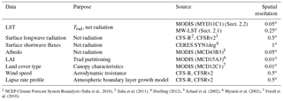
² NCEP Climate Forecast System Reanalysis (Saha et al., 2010), ³ Saha et al. (2011), ⁴ Doelling (2012), ⁵ Schaaf et al. (2002), ⁶ Myneni et al. (2002), ⁷ Friedl et al. (2010).

Figure 1 MW-LST workflow.

2.2 Temperature from MODIS

The MODIS instrument on the polar-orbiting Aqua satellite (July 2002 to present) with an equator overpass time of 13:30 and 01:30 LST provides global TIR observations with spectral bands suitable for estimating LST. The specific LST product used for the ALEXI implementation is the MODIS Climate Modeling Grid 0.05^∘ daily LST product (MYD11C1 Wan, 2008), which is distributed by the Land Processes Distributed Active Archive Center (https://lpdaac.usgs.gov). Although the overpass times of this satellite do not correspond directly with ALEXI's time 1 and time 2, Hain and Anderson (2017) show that, over the US, GOES-based ΔT_rad can be estimated with a 5–10 % relative error using a tree-based regression model based on independent variables including vegetation index and land cover class. This regression model, trained over the GOES domain, is then applied globally to estimate T_rad at time 1 and time 2 from MODIS LST.

2.3 Temperature from a constellation of MW satellites

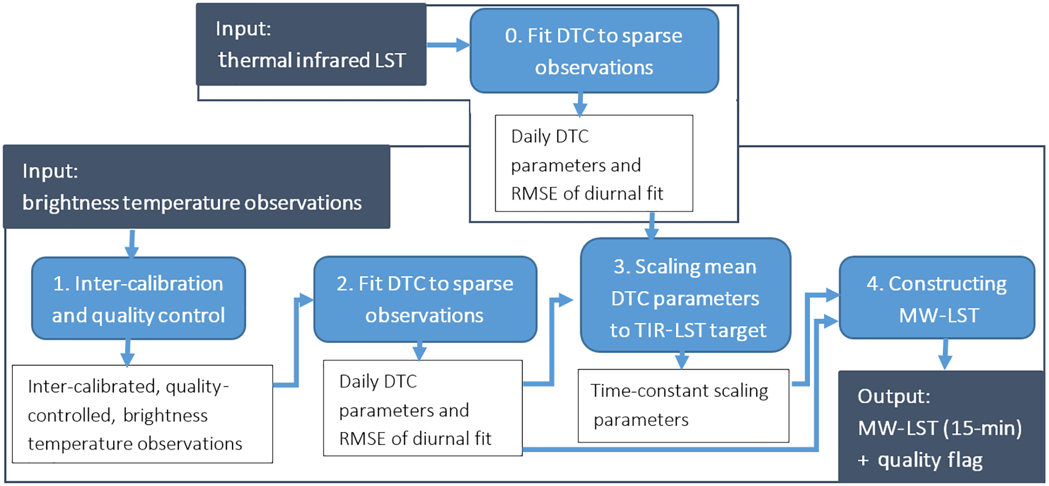
The MW-LST product is based on vertical polarized Ka-band (36–37 GHz) brightness temperature (T^Ka), a spectral band commonly included in multi-frequency microwave radiometers in low-Earth orbit. The current MW-LST product integrates observations from six of these satellites. Most important are the Advanced Microwave Scanning Radiometer EOS (AMSR-E) on Aqua from mid-2002 to October 2011 and its successor AMSR2 on the Global Change Observation Mission 1st Water (GCOM-W) from July 2012 onward. Also included are the Special Sensor Microwave and Imager (SSM/I) on platforms F13–F15 of the Defense Meteorological Satellite Program, the Tropical Rainfall Measuring Mission (TRMM) Microwave Imager (TMI) and Coriolis–WindSat. Together this constellation of Ka-band radiometers allows for the estimation of the diurnal temperature cycle in a process that can be summarized in 4-steps, detailed below and diagrammed in Fig. 1.

2.3.1 Inter-calibration of MW satellites

All available Ka-band observations are combined to create a global record with up to 8 observations per day for each 0.25^∘ resolution grid box. The data are binned in 15 min windows of local solar time (00:00–00:15 LST is the first window of the day). The brightness temperatures are inter-calibrated using observations from the TRMM satellite (with an equatorial overpass) as a transfer reference. Individual 0.25^∘ averages are masked if the spatial standard deviation of the oversampled Ka-band observations exceeds a prior determined threshold for each grid box. Both the inter-calibration and quality control procedures are described in detail in Holmes et al. (2013a). The resulting global record of inter-calibrated Ka-band brightness temperatures spans the years 2003–2013.

2.3.2 Fitting of diurnal cycle model to sparse observations

For days with suitable MW observations (a minimum of 4, at least one of which is close to solar noon) and no T^Ka < 250 K (an indication of frozen soil), a continuous diurnal temperature cycle is fitted. The DTC model combines a cosine and an exponential term to describe the effect of the sun and the decrease in surface temperature at night and is based on Göttsche and Olesen (2001) with slight adaptations to limit the number of parameters. This implementation (DTC3) is fully described in Holmes et al. (2015). DTC3 summarizes the DTC with four parameters: daily minimum (T₀) at start and end of day, diurnal amplitude A and diurnal timing φ. The fitting procedure first determines φ as a temporal constant (Holmes et al., 2013b) and subsequently T₀ and A for each day individually. The success of the fit (ε_d) is expressed as the root mean square error (RMSE) between the modeled and observed T^Ka for the n observations (at times t) in any given day (d), calculated following Eq. (1):

$$\begin{array}{}\text{(1)}& {\displaystyle }{\displaystyle }{\mathit{\epsilon }}_d=\sqrt{{\displaystyle \frac{\mathrm{1}}{n}}\sum _{i=\mathrm{1}}^n{\left(T_i-\mathrm{DTC}\mathrm{3}\left(\mathit{\phi },T_{\mathrm{0}},A,t_i\right)\right)}^{\mathrm{2}}}.\end{array}$$

This method was applied to the entire record of inter-calibrated Ka-band brightness temperatures (Sect. 2.3.1) to create a database of annual maps of φ^Ka and daily maps of $T_{\mathrm{0}}^{\mathrm{Ka}}$ and A^Ka

2.3.3 Scaling of MW DTC parameters to match the TIR-LST target

To relate the diurnal cycle in Ka-band brightness temperature to the composite radiative temperature of the land surface requires a set of DTC parameters that is equivalent to those derived from T^Ka but derived from a TIR-LST product. In the present analysis, the TIR-LST that serves as a reference is produced at the Land Surface Analysis Satellite Application Facility (LSA-SAF). The LSA-SAF LST is based on TIR window channels of SEVIRI (Spinning Enhanced Visible and Infrared Imager) onboard the Meteosat Second Generation (MSG) geostationary satellite. The same method for fitting a DTC model to sparse observations (Sect. 2.3.2) was applied to the LSA-SAF LST to create a database of annual maps of φ^TIR and daily maps of $T_{\mathrm{0}}^{\mathrm{TIR}}$ and A^TIR (Holmes et al., 2015). This preparation step is diagrammed in Fig. 1 as step “0”.

The Ka-band DTC parameters ($T_{\mathrm{0},d}^{\mathrm{Ka}}$, $A_d^{\mathrm{Ka}}$) are scaled so that the long-term mean matches that of the equivalent TIR-based parameters ($T_{\mathrm{0},d}^{\mathrm{TIR}}$, $A_d^{\mathrm{TIR}}$). Because $T_{\mathrm{0}}^{\mathrm{Ka}}$ is affected by the sensing depth, the scaling is performed by using daily mean temperature as an intermediate, which is defined as (${\stackrel{\mathrm{‾}}{T}}^{\mathrm{Ka}}$ = $T_{\mathrm{0}}^{\mathrm{Ka}}$ + A^Ka∕2) for this purpose.

$$\begin{array}{}\text{(2)}& {\displaystyle }& {\displaystyle }{A}_d^{\mathrm{MW}}=A_d^{\mathrm{Ka}}/\mathit{\delta }\text{(3)}& {\displaystyle }& {\displaystyle }{\stackrel{\mathrm{‾}}{T}}_d^{\mathrm{MW}}={\mathit{\beta }}_{\mathrm{0}}+{\mathit{\beta }}_{\mathrm{1}}{\stackrel{\mathrm{‾}}{T}}_d^{\mathrm{Ka}}\end{array}$$

The scaled parameters are indicated with the superscript “MW”. The parameter δ represents the slope of the zero-order least-squares regression line for estimating the amplitude of $A_d^{\mathrm{Ka}}$ from TIR-LST ($A_d^{\mathrm{TIR}}$). The intercept (β₀) and slope (β₁) to correct the mean daily temperature (${\stackrel{\mathrm{‾}}{T}}_d^{\mathrm{Ka}}$) for systematic differences with TIR-LST (${\stackrel{\mathrm{‾}}{T}}_d^{\mathrm{TIR}}$) are determined with a constrained numerical solver, as in Holmes et al. (2015). The constraint is based on radiative transfer considerations and assures that the scaling of the mean is in agreement with the prior scaling of the amplitude (Eq. 2).

The set of time-constant scaling parameters (δ, β₀ and β₁) were determined for each 0.25^∘ grid box based on all days in the period 2007–2012 where both MW- and TIR-based DTC parameters were available (generally clear sky and above freezing). Because all three parameters are constant with time, Eqs. (2–3) preserve their temporal independence of the TIR-LST product. The consequence of using LSA-SAF LST as the reference product is that observation-based scaling parameters are limited to the domain covered by Meteosat (Africa, Europe, Middle East). Outside this domain, the parameters must be extrapolated. The procedure for the extrapolation is still in development and currently entails fitting linear regressions with vegetation characteristics. Because of the limited confidence in the scaling parameters outside the MSG domain, the analysis in this paper is focused on the Africa and Europe domain. Some results of the global set will be presented in the comparison with flux-tower observations (Sect. 3.4).

2.3.4 Constructing MW-LST

Global maps of the time-constant parameters (δ, β₀ and β₁; Sect. 2.3.3) are used to calculate the daily DTC parameters ($T_{\mathrm{0},d}^{\mathrm{MW}}$, $A_d^{\mathrm{MW}}$) in the scaled climatology of the TIR-LST product. This scaling (Eqs. 2 and 3) is applied to every day for which estimates of ${\stackrel{\mathrm{‾}}{T}}^{\mathrm{Ka}}$ and A^Ka are available (see Sect. 2.3.2). The methodology to scale the DTC parameters from this record of Ka-band observations to a physical temperature range is described in more detail in Holmes et al. (2015). The scaled parameters together with φ^TIR are then used to construct MW-LST based on the same DTC3 model as used in step 2:

$$\begin{array}{}\text{(4)}& {\displaystyle }{\displaystyle }\mathrm{MW}-{\mathrm{LST}}_i=\mathrm{DTC}\mathrm{3}\left({\mathit{\phi }}^{\mathrm{TIR}}{T}_{\mathrm{0},d}^{\mathrm{MW}},A_d^{\mathrm{MW}}\right).\end{array}$$

The use of the DTC model allows MW-LST to be diurnally complete for days when both $T_{\mathrm{0},d}^{\mathrm{MW}}$ and $A_d^{\mathrm{MW}}$are available. MW-LST can therefore be generated at any time increment (i). The MW-LST database used for this paper was generated at a 15 min temporal interval. This allows T_rad1 and T_rad2 to be accurately interpolated from the database. ${\mathit{\epsilon }}_d^{\mathrm{Ka}}$ (Eq. 1) is used to flag days where the assumptions imposed by the shape of clear-sky DTC3 are not valid or individual Ka-band observations have a large bias. In this experiment, MW-LST was only used if ${\mathit{\epsilon }}_d^{\mathrm{Ka}}$ was 2.5 K or lower.

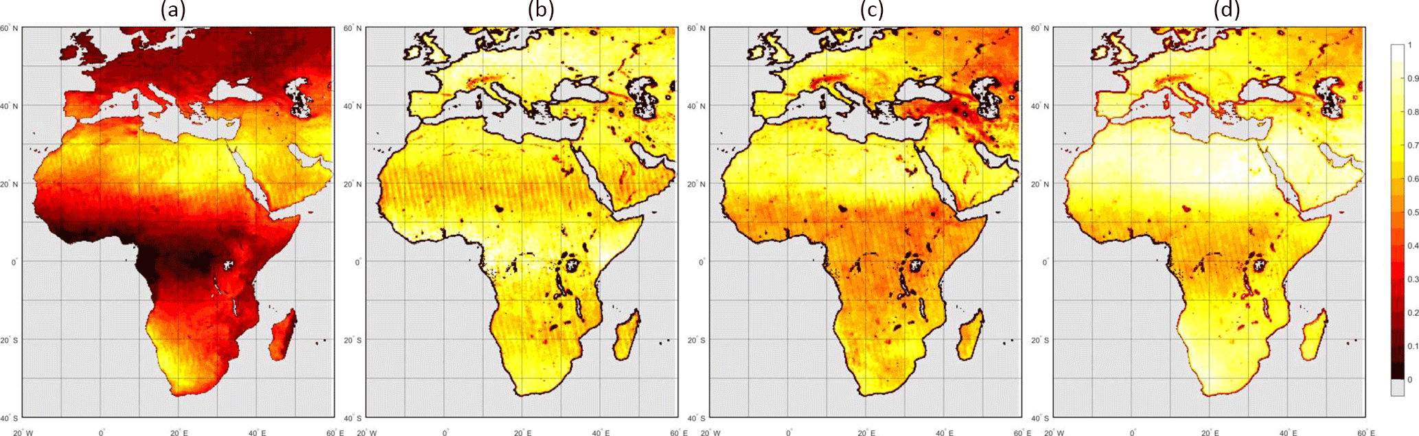
Figure 2 Temporal coverage of MW- and IR-based ΔT_rad in 2004. (a) shows the fraction of total days where MODIS-based estimates of ΔT_rad are available. (b) shows the fraction of this subset of days where there is also a MW-based ΔT_rad available. (c) shows the fraction of days without a MODIS-based estimate but with availability of a MW-based estimate (potential for IR-gap coverage). (d) shows the fraction of total days where either a MODIS- or a MW-based ΔT_rad is available.

2.3.5 MW-LST in ALEXI

The continuous 7-day totals are achieved by temporal gap-filling of (clear sky) ET as a fraction of clear-sky latent heat flux to incoming solar radiation (Anderson et al., 2007a). To maximize similarity, the same MODIS cloud mask is applied to the ALEXI-MW implementation so that the mechanics of standard ALEXI can be evaluated under circumstances for which it has previously been developed and validated.

The fraction of days in a year where a clear-sky MODIS-based T_rad1 and T_rad2 is available for ALEXI is below 0.3 for large parts of Europe and (sub)-tropical Africa (Fig. 2a). In these areas the revisit time between observation days regularly exceeds 5 days, which is a threshold for temporal downscaling given the persistence of ET fraction (Alfieri et al., 2017). On average for the non-coast pixels, there is a MW-based estimate available for 69 % of those days where there is also a (clear sky) MODIS-based T_rad1 and T_rad2. The reason this percentage is not higher is mainly due to the requirement of a near-noon overpass for the fitting of the diurnal temperature curve (see Sect. 2.3.2), in combination with the 1 in 3 days without such overpass for a given location as determined by the orbit and coverage of Aqua and GCOM-W. The multi-year and global record of simultaneous MW-LST and MODIS LST during clear skies will support further calibration of MW-LST to MODIS LST in future investigations. This MW to MODIS calibration was not done in this study but is likely needed to maximize consistency between ALEXI implementations over the globe. In terms of potential for additional sampling through the use of MW-based LST, Fig. 2c shows that MW-based estimates for the two ALEXI times are available for 54 % of the days where no MODIS-based estimate is available. Figure 2d depicts the fraction of days where either MODIS or MW-LST can be used to estimate the T_rad inputs required to run ALEXI. This shows that the addition of MW-LST can bring the minimum average coverage in this domain to once every 2 days.

2.4 Flux-tower observations

Tower measurements of latent heat flux obtained using the eddy-covariance technique are commonly used for ground truthing of remote sensing and model-based ET estimates (Baldocchi et al., 2001). Harmonized Fluxnet data are distributed in so-called synthesis datasets. They include the original observations at a 30 min observation time and aggregate values per day, week and month. For this work, we used the synthesis 2015 Tier 1 data as accessed in July 2016 (http://fluxnet.fluxdata.org/data/fluxnet2015-dataset/) to serve as a common ground reference for the evaluation of the temporal characteristics of ALEXI-MW and ALEXI-IR. In particular, the part of the dataset of interest here is the daily aggregates of latent heat flux (variable name LE_F_MDS) which include quality control as described in Pastorello et al. (2014).

Based on these daily data, we computed the 7-day averages matching the window length of ALEXI. If not all days within a window have valid data, that window is disregarded. Overall, eddy-covariance observations of ET were available from 68 flux towers with at least 1 year of observations within the time period of this study.

Figure 3 Location of flux-tower sites used in the analysis (see also Table 2): (a) North America, (b) Europe and (c) the world. The size of the marker is in proportion to the number of data days used in the assessment. (d) indicates the 11 regions selected based on annual precipitation cycle and geographic diversity.

2.5 Definition of regions

Although both MW and IR sets are available globally, the main analysis of this paper is focused on the domain encompassing Africa and Europe. This is because only in that region is the scaling of MW-LST to TIR-based LST currently supported by data (see Sect. 2.3.3). However, temporal comparisons (e.g., correlations) are much less affected by the mean absolute value of the MW-LST product. Because of the limited availability of flux-tower data, we include all available stations from across the globe which allows us to double the amount of stations available for the analysis compared to only the sites in Europe and Africa.

Within the main focus domain of this study we further highlight 11 climate-based domain subsets (see also Fig. 3, bottom-right panel):

• A.

  West-African Sahel, arid;

• B.

  West-African Sahel, semi-arid;

• C.

  Guinean coast, dry subhumid;

• D.

  Central Africa, humid;

• E.

  Horn of Africa, arid;

• F.

  Southern Africa, semi-arid (large bias in Fig. 4);

• G.

  Southern Africa, arid (large bias in Fig. 4);

• H.

  Iberia, semi-arid;

• I.

  Germany, continental humid;

• J.

  European Russia, continental humid, boreal forest (large bias in Fig. 4);

• K.

  France, humid.

These regions are selected to represent a wide variety of seasonal variation in precipitation and climate class and are based on the work of Trambauer et al. (2014). Rather than attempting to cover the entire domain with these subsets, we selected smaller subsets in order to visualize the local deviations between MW and IR products that might otherwise be averaged out. We also added regions in Europe and several regions that showed a large bias in Fig. 4.

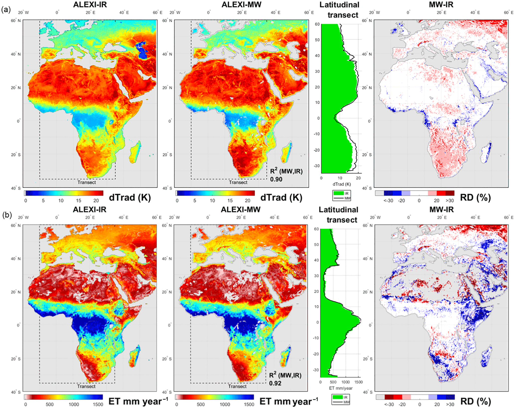
Figure 4 Multi-year mean of clear-sky ΔT_rad (a, 2004–2011) and mean annual clear-sky ET (b, 2003–2011) for IR and MW. The transect shows the latitudinal average for longitude 10^∘ W to 35^∘ E. The right-hand panel shows the corresponding relative difference (RD) between the two estimates (MW–IR), with areas with ET below 14 mm month⁻¹ greyed out. Note the reversed color bars for ΔT_rad and ET to emphasize their negative correlation (ΔT_rad up, ET down). ΔT_rad is defined in the ALEXI framework as the temperature rise between 1.5 h after sunrise to 1.5 h before noon (see Sect. 2.1).

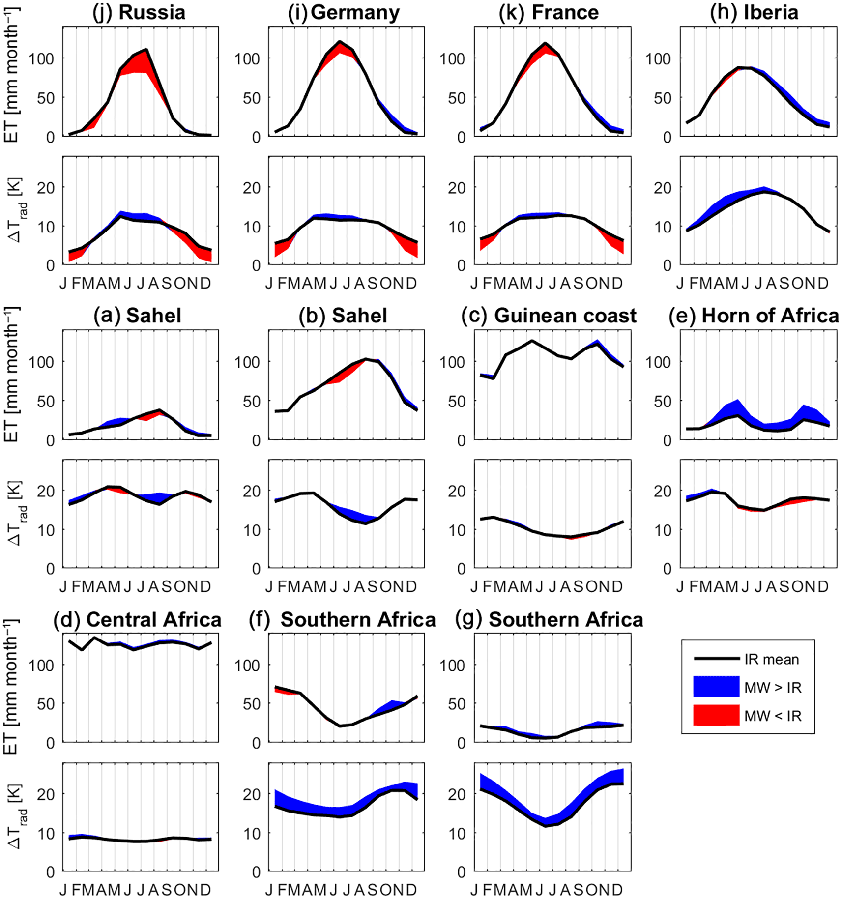
Figure 5 Mean monthly ET as estimated with ALEXI-IR over 2003–2011, and monthly means of its MODIS-based ΔT_rad input (period 2004–2011), for selected regions. The deviation from these IR estimates when using the MW inputs is shown in blue for a positive deviation and red for a negative deviation.

2.6 Metrics

Cumulative annual and seasonal fluxes are compared in terms of their relative difference – RD (%), calculated following Eq. (5):

$$\begin{array}{}\text{(5)}& {\displaystyle }{\displaystyle }\mathrm{RD}={\displaystyle \frac{\stackrel{\mathrm{‾}}{x}-\stackrel{\mathrm{‾}}{y}}{\left(\stackrel{\mathrm{‾}}{x}+\stackrel{\mathrm{‾}}{y}\right)/\mathrm{2}}}\times \mathrm{100}\mathit{\%},\end{array}$$

where $\stackrel{\mathrm{‾}}{x}$ represents the mean of the MW product and $\stackrel{\mathrm{‾}}{y}$ the mean of the IR product, both sampled at the same times. This relative comparison is useful because neither product represents the truth and this formulation places the difference in the context of the size of the fluxes. Still, if the ET is very small (average ET below 14 mm month⁻¹) then the denominator becomes too small and the RD is not reported. The temporal agreement between the anomalies in the IR and MW-based ET products is analyzed in terms of the Pearson's correlation (ρ) and the spatial agreement in terms of the correlation coefficient (R²).

The temporal agreement of the weekly ET estimates is further compared relative to the flux-tower observations that serve as a common reference. For this assessment, MW- and IR-based ET estimates are again compared in terms of ρ but also in terms of root mean square error to quantify the absolute error. The RMSE is calculated following Eq. (7):

$$\begin{array}{}\text{(6)}& {\displaystyle }{\displaystyle }\mathrm{RMSE}=\sqrt{{\displaystyle \frac{\mathrm{1}}{N}}\sum (x-y{)}^{\mathrm{2}}},\end{array}$$

where x is the satellite estimate of ET and y is the tower-based measurement of ET. N is the number of data pairs.

3 Results

3.1 Comparing multi-year means

The mean average ΔT_rad as calculated from MW-LST deviates from that calculated from MODIS LST by 0–20 %, which leads to a spatial R² of 0.90 (Fig. 4, top row panels). These spatial variations in mean values arise from the different calibration targets. MW-LST is calibrated to match the LSA-SAF LST from MSG (Europe and Africa) with a precision of 2–3 K (see Sect. 2.3.3), and MODIS ΔT_rad is trained on GOES (North America) with an estimated precision of 5–10 % (see Sect. 2.2). These different calibration domains together with likely calibration differences between GOES and MSG LST products present sources of bias that can explain the regional variation we see in Fig. 4. For example, the difference between ΔT_rad estimates in the northeast corner of this map may be an artifact of scaling with high incidence angles (θ) for the MSG geostationary satellite. In the farthest corner (θ > 60^∘), MSG observations were not used and the MW scaling is extrapolated based on land surface characteristics. The MW ΔT_rad also exceeds IR-based estimates by more than 10 % in Southern Africa, for which we do not currently have an explanation.

The general agreement in mean ΔT_rad translates into a high agreement between IR and MW-based ALEXI in terms of mean annual ET for the period 2003–2011. The spatial correlation between MW and IR in terms of ET is 92 % (Fig. 4, bottom row panels), similar to that for ΔT_rad. Boreal Russia shows the most notable differences in absolute terms, where MW is lower by ∼ 20 %. This is related to view angle impacts on the ΔT_rad retrieval, as noted above. MW ET is also much lower than IR ET in the Alps, which likely reflects an interaction between view angle and topography (e.g., differences in pixel proportion of sunlit and shaded slopes). In the Horn of Africa, MW is higher by 20–30 %, although little difference in ΔT_rad is apparent in this region. ALEXI ET becomes more sensitive to small changes in ΔT_rad near the dry end, where the iterative stress reduction in transpiration starts to kick in.

3.2 Regional and seasonal bulk flux comparison

Figure 5 provides a more detailed comparison between the MW and IR products for the domain subsets as described in Sect. 2.5. For each domain subset, it shows the mean monthly total ET and the associated monthly means of ΔT_rad. For European Russia (region J) and to a lesser extend Germany (I) and France (K), this shows a higher MW-based ΔT_rad resulting in lower summertime ET estimates than for ALEXI-IR. Conversely, in the wintertime the lower MW-based ΔT_rad results in higher ET estimates compared to the TIR products in October–December. For Iberia (H), the semi-arid Sahel (B) and Spain (H) there appears to be a difference in timing with MW estimating a later time for peak ET. The higher MW ET estimates in the Horn of Africa are rather uniform over the year, except for December and January where the difference is small. The size of the bias in ET for the Horn of Africa is relatively large compared to the modest bias in ΔT_rad. Another disconnect between ΔT_rad deviation and ET can be seen in Southern Africa (regions F and G). Despite a general overestimation of ΔT_rad by MW, the ET estimates are very close to those of ALEXI-IR. The small difference in ET estimates are the opposite of what would be expected from the ΔT_rad deviation. Finally, the humid tropical climates of the Guinean coast and Central Africa (regions C and D) have very little differences in both ΔT_rad and ET.

To provide some additional spatial and temporal context for these observations, the 3-month total MW and TIR ET (averaged over 2003–2011) are shown in Fig. 6 for December–January–February (DJF), March–April–May (MAM), June–July–August (JJA) and September–October–November (SON). This shows that the cold season overestimation of MW-based ET, seen in the European regions, is present not only in Europe but also in eastern and Southern Africa in SON. The underestimation of MW-based ET in summer is not as pronounced in terms of its relative difference. The apparent difference in timing, seen in the Sahel and Iberian regions, shows up across the southern border of the Sahara – MW ET is higher in MAM, and TIR ET is higher in JJA. The spatial correlation between MW and IR is higher in SON (96 %) and DJF (97 %) compared to the periods MAM (83 %) and JJA (84 %). Despite these localized differences, the transect averages are remarkably similar showing the general success of scaling MW-LST to TIR-LST (Sect. 2.3.3).

Figure 6 As Fig. 4, but now averaged by season.

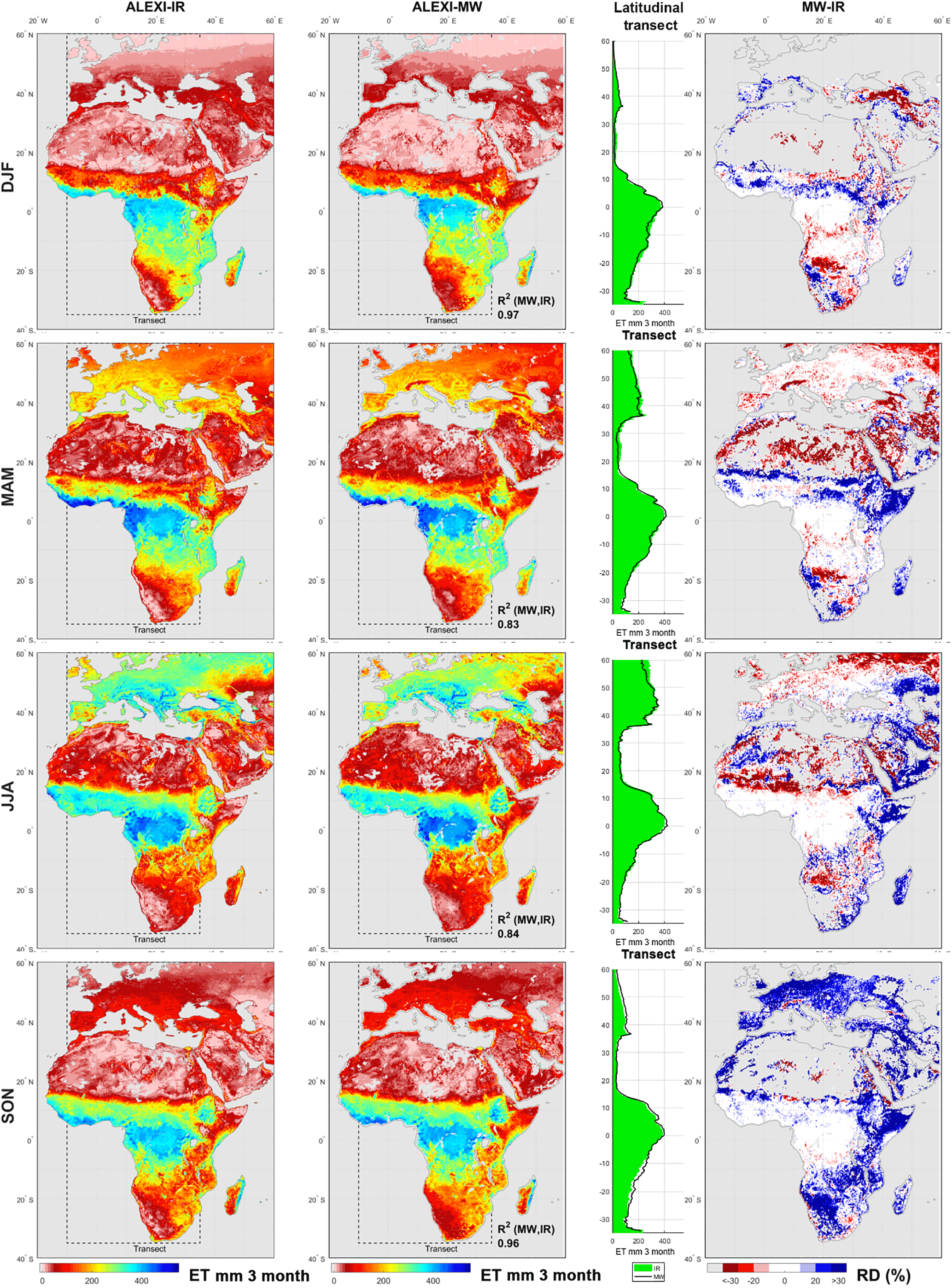
Table 2 Time-series correlation of flux-tower ET observations with three alternative satellite-based ET estimates (ALEXI-IR, ALEXI-MW, ALEXI-IR + MW). Comparison is based on weekly averages in the period of 2003 to 2011 (number of data pairs is noted in the table). Bias is the mean difference between the 0.05 grid and 0.25 surrounding grid average as measured by ALEXI-IR. NA = not available.

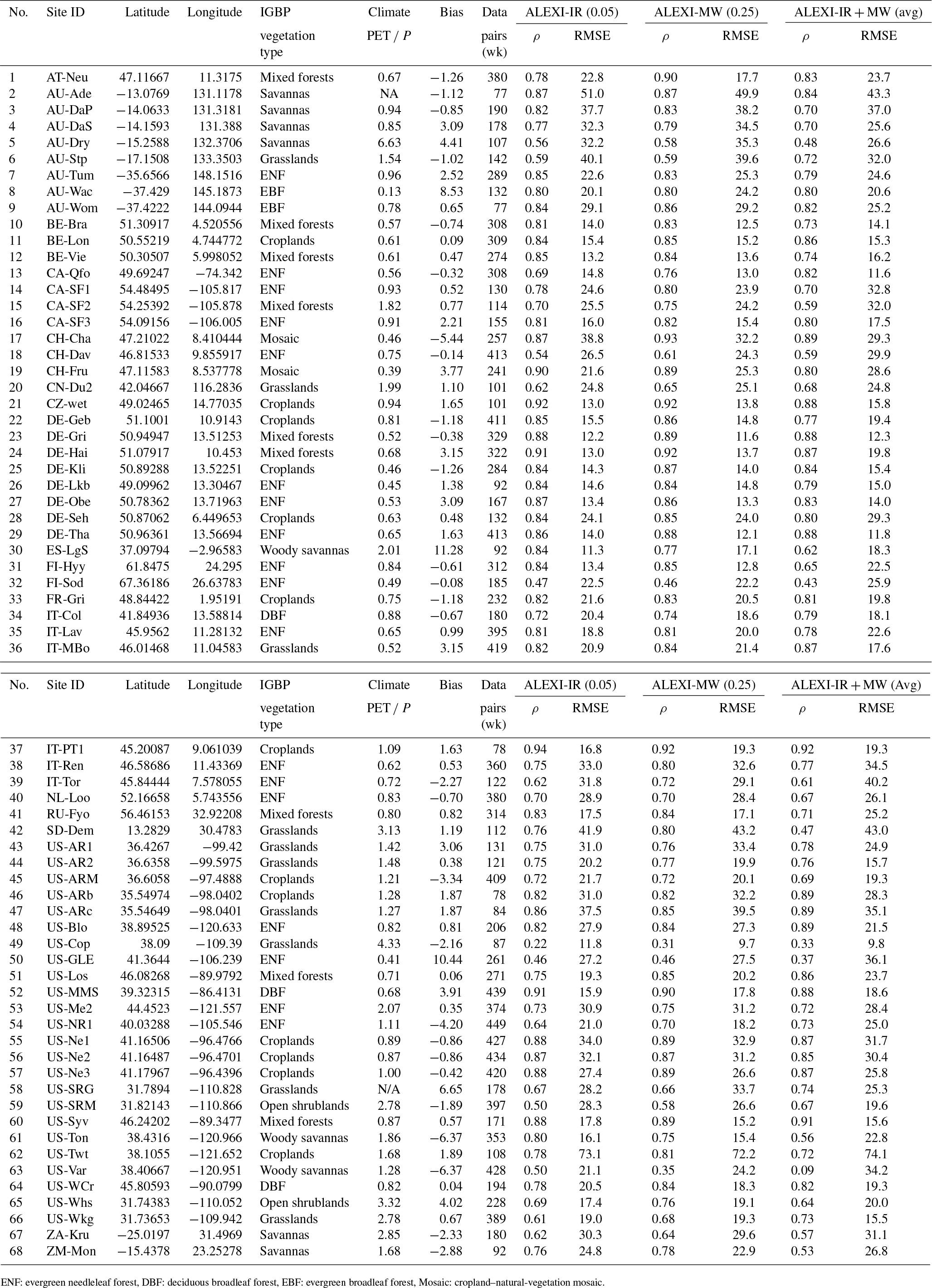
ENF: evergreen needleleaf forest, DBF: deciduous broadleaf forest, EBF: evergreen broadleaf forest, Mosaic: cropland–natural-vegetation mosaic.

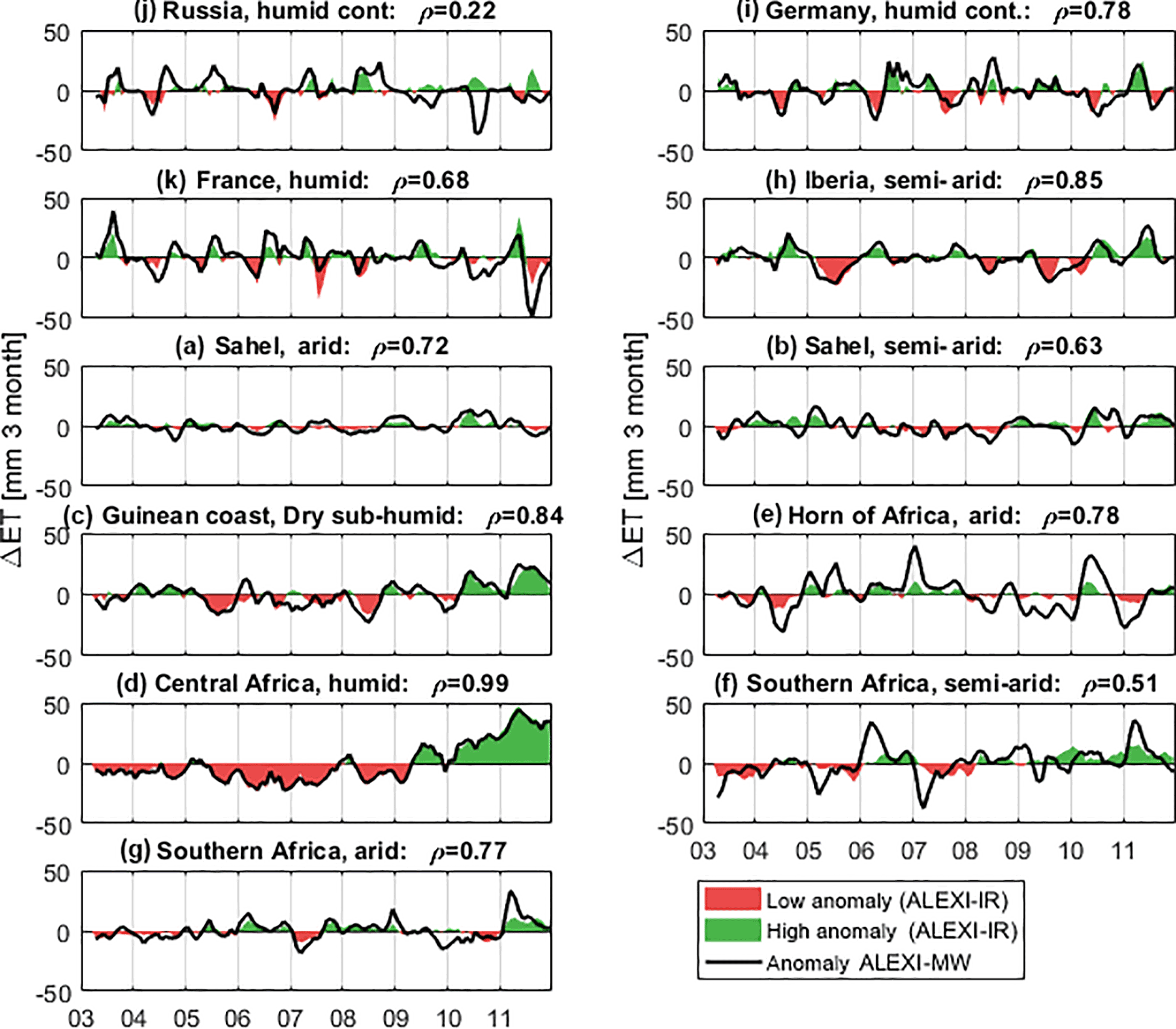
Figure 7 Comparison of anomaly in 3-month ET totals as calculated from ALEXI-IR and ALEXI-MW for selected regions (see Fig. 3 for definition of regions).

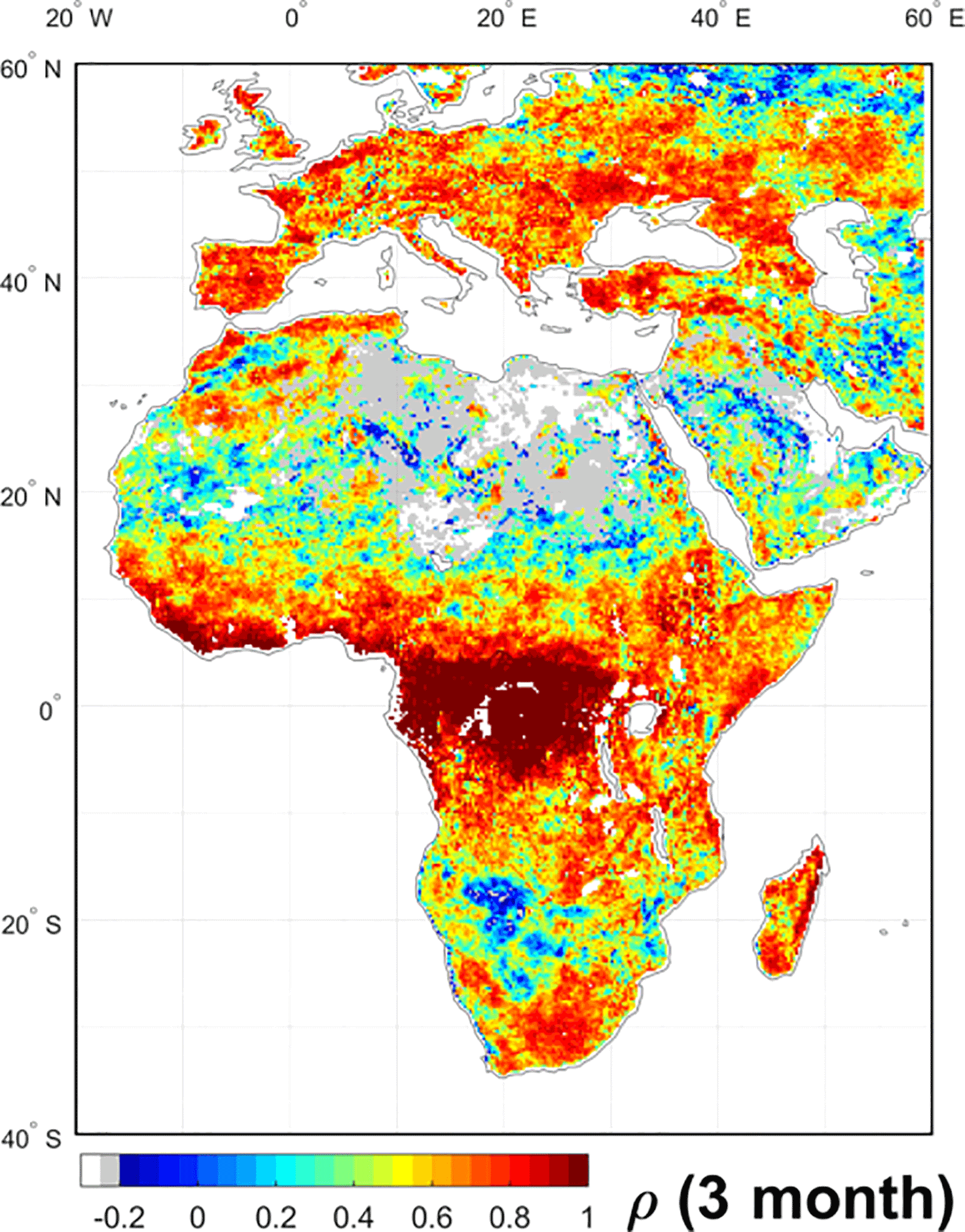
Figure 8 Pearson's correlation between anomaly in 3-month ET totals as estimated by ALEXI-IR and ALEXI-MW, calculated at 0.25^∘ resolution. White areas have no data; grey areas are masked because the standard deviation in the 3-month anomaly was below 8 mm/3 months in both estimates.

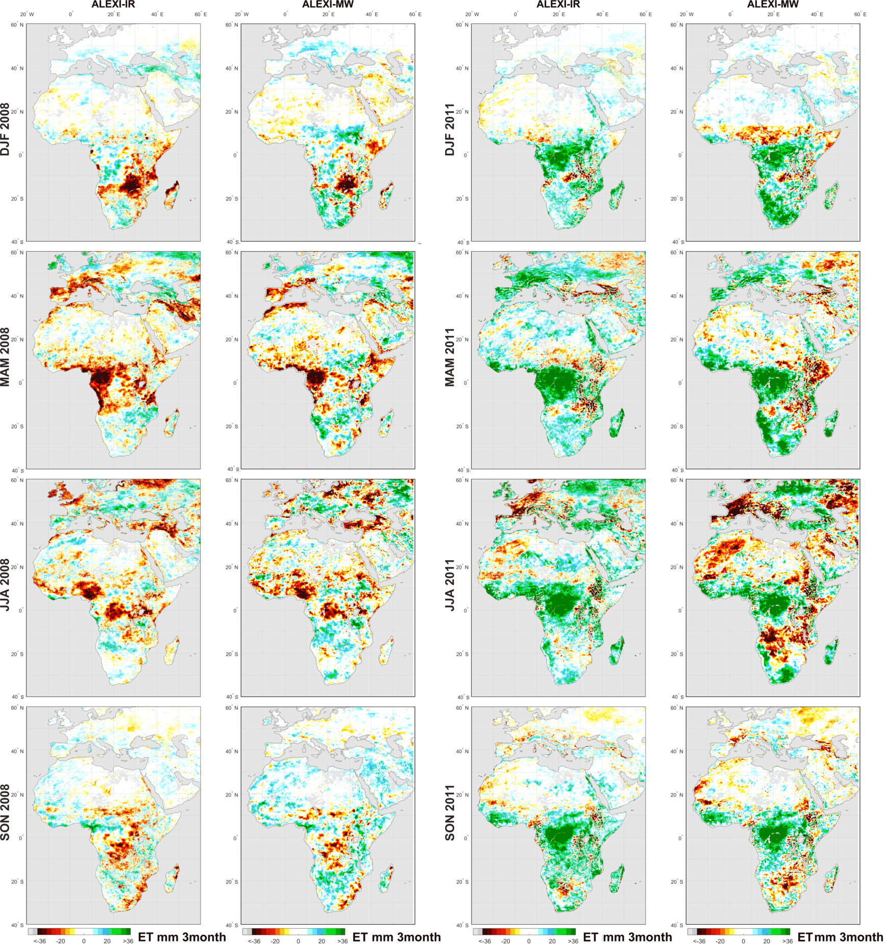
Figure 9 Anomaly in seasonal ET compared to multi-year mean (2003–2011, see Fig. 6) as retrieved by ALEXI-IR and ALEXI-MW. The first two columns show the anomalies for 2008 and the two right-hand columns show them for 2011.

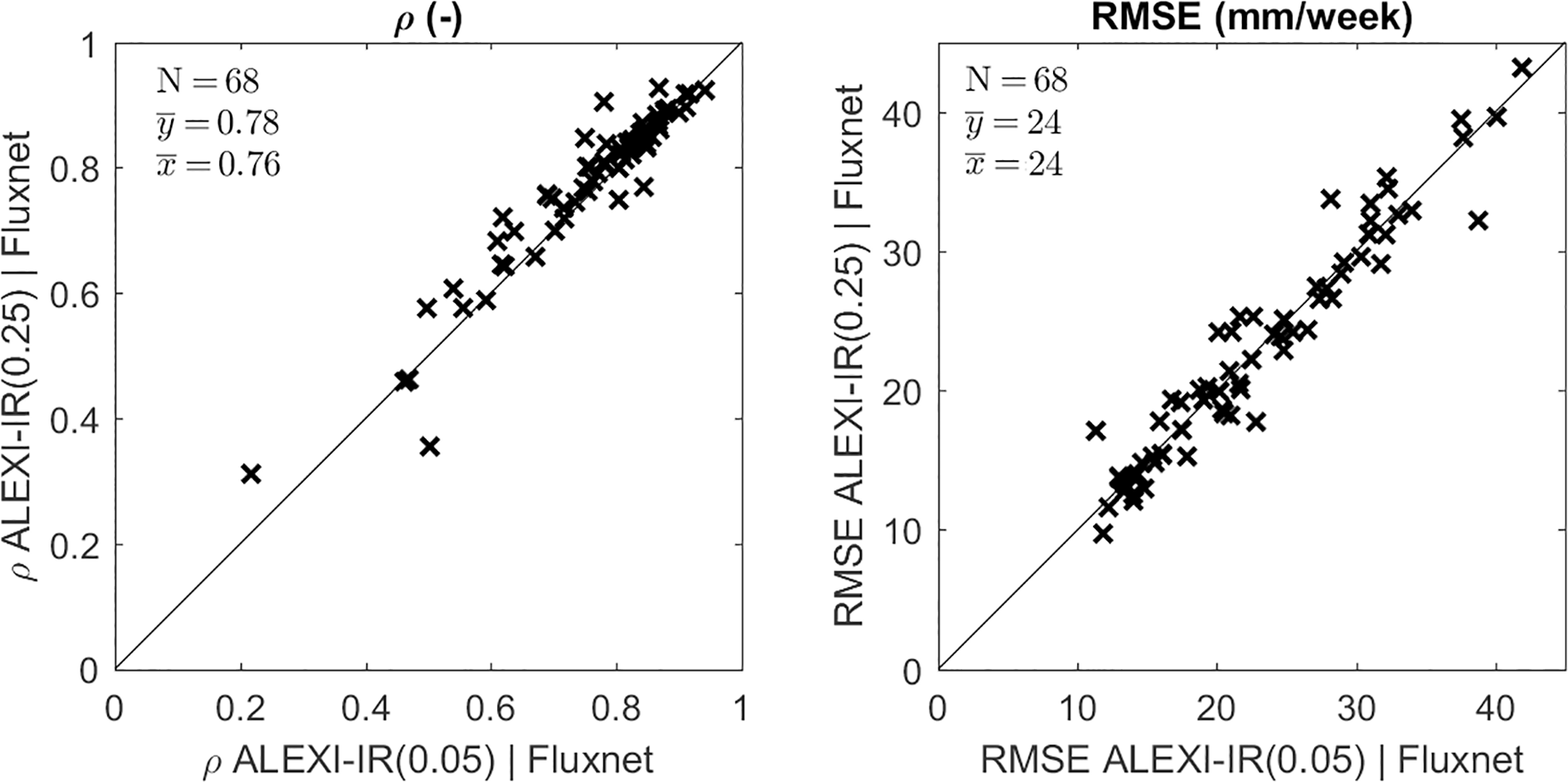
Figure 10 The effect of spatial resolution in the satellite product on Pearson correlation (ρ) and RMSE between weekly ET estimates from satellite data (ALEXI-IR) and flux-tower eddy-covariance measurements (Fluxnet). Each marker represents a single station and compares results at the original 0.05^∘ resolution of ALEXI-IR (x axis) with those calculated for 0.25^∘ resolution ALEXI-IR (y axis).

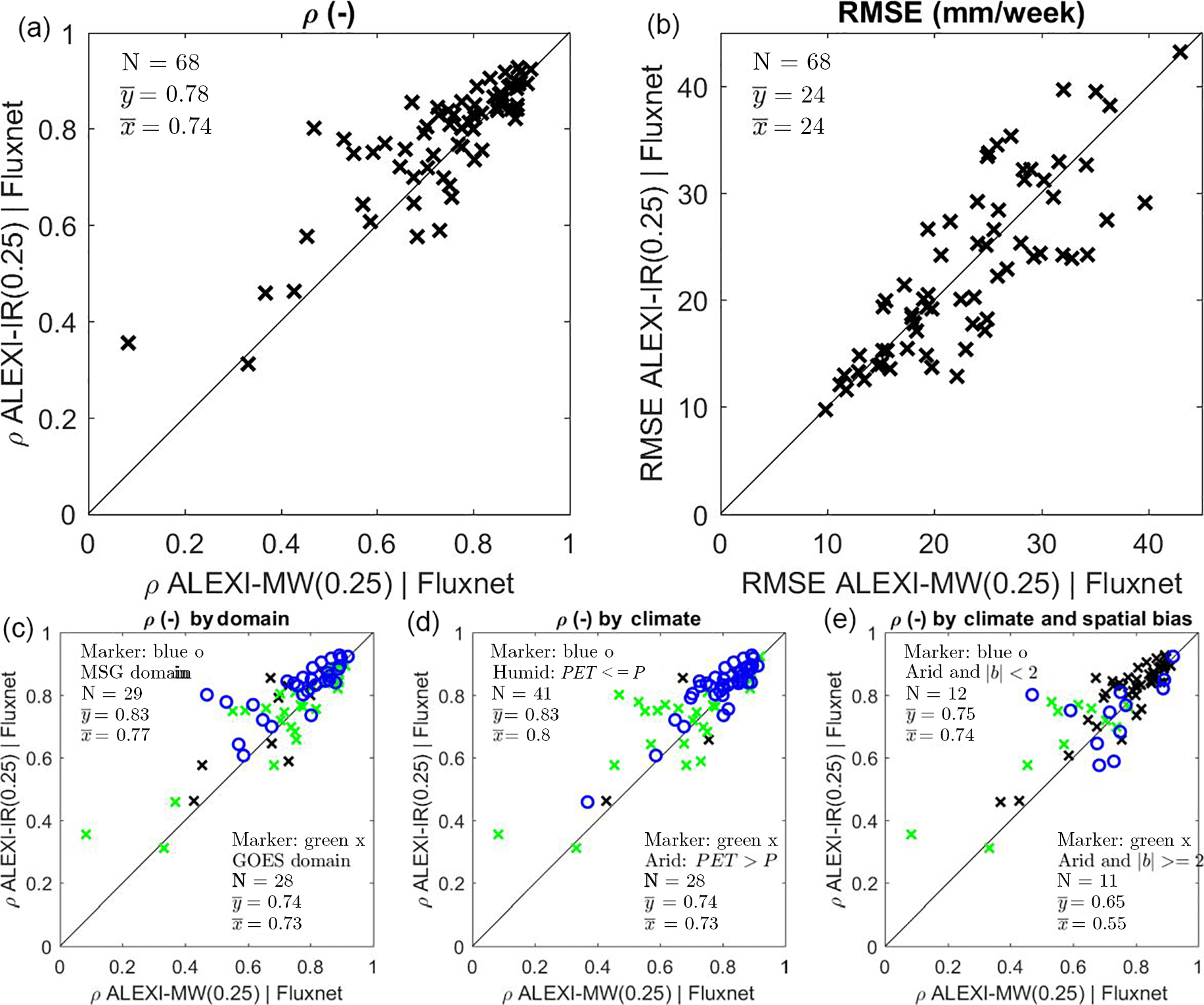
Figure 11 The effect of switching from TIR to MW-LST as input to ALEXI on Pearson correlation (ρ) and RMSE between weekly ALEXI ET estimates and flux-tower eddy-covariance measurements (Fluxnet). Each marker represents a single station and compares results calculated for ALEXI-MW (x axis) with those calculated for ALEXI-IR (y axis). (c)-(e) Same data as presented in (a), but now distinct subsets of the tower sites are emphasized. (c) Sites by geographic region; (d) sites grouped by climate (humid vs. arid, see text for definition). (e) splits the arid sites further based on bias between the ALEXI-IR (0.05^∘) and the mean value for the encompassing 0.25^∘ grid box with a threshold of $\left|b\right|$ = 2 mm week⁻¹. The black x mark stations that are either below 60^∘ N or are not covered by the two contrasting selections.

3.3 Inter-annual variation

Because the long-term mean of MW-LST is calibrated to match a TIR reference (see Sect. 2.3.3), a comparison in terms of anomalies is the real test of its performance in the ALEXI framework, especially in areas that are water limited (see Fig. 7). Of the subsets in water-limited regions, the Horn of Africa (ρ = 0.78) and Spain (ρ = 0.85) subsets show a high degree of correlation between MW- and TIR-based ET anomalies. Semi-arid Southern Africa (F) and the Sahel (B) show relatively poor correlation with ρ = 0.48 and ρ = 0.63 respectively. The size of the anomaly is much larger for ALEXI-MW in Southern Africa in January and February, reflecting a much larger inter-annual variation.

In energy-limited areas when ET is fully determined based on the meteorological forcing data, the effect of LST inputs is minimal. This is apparent in the Tropical region, where MW and ALEXI-IR have a correlation of 0.99 in Central Africa (region D). Figure 8 shows a map of the correlation between 3-month anomalies of MW- and IR-based ALEXI ET.

Seasonal anomalies are calculated by taking the seasonal total ET for a given year and subtracting its corresponding long-term mean seasonal total (2003–2011 period, as shown in Fig. 6). Examples of this are shown for a dry year (2008) and a wet year (2011), see Fig. 9. Overall the two sets of anomalies agree very well – the MW ALEXI appears to identify roughly the same areas with anomalous high or low ET. The agreement is better in the wet year than in the dry year.

3.4 Comparison with flux-tower observations

The availability of eddy-covariance observations of ET from 68 flux towers allows for a more detailed grid-level analysis of temporal agreement. Even at the 0.05^∘ (∼ 5 km) resolution of ALEXI-IR there is a large-scale mismatch between the remote sensing estimate and tower footprint. The impact of this scale difference will depend on the degree of spatial heterogeneity within the larger footprint. We therefore cannot use these flux-tower observations to quantify absolute accuracy in either product, but instead focus on its use as a reference target to compare relative performance between two satellite products. To start, we compare the effect of the resolution degradation from 0.05 to 0.25^∘.

When 0.05^∘ ALEXI-IR is averaged over its surrounding 0.25^∘ grid (the average of the 5 × 5 0.05^∘ grid cells), there is an overall improvement in ρ (but not in RMSE), see Fig. 10. Only at three sites does this spatial degradation of the remote sensing measurement lower its ρ with the site measurement. The landscape heterogeneity is large at these sites (US-Ton, US-Var and ES-Lgs). For most stations, the spatial degradation actually improves the ρ with the site. In fact, 40 % of the difference in ρ between the MW and IR implementations of ALEXI is explained by the change in ρ resulting from the averaging of ALEXI-IR at 0.05^∘ to 0.25^∘ spatial resolution. This indicates the presence of noise in the 0.05^∘ MODIS-LST input that is uncorrelated with the surrounding 0.25^∘ grid average and negates any positive effect of its resolution advantage compared to a 0.25^∘ grid average for most sites.

The following analysis compares MW and IR both at 0.25^∘ grid resolution. The metrics we focus on are ρ and RMSE which are computed for each flux-tower site and listed in Table 2. For ALEXI-IR, ρ is between 0.6 and 0.92 and RMSE is 12–33 mm week⁻¹ for the majority of the sites. The impact of LST input varies from site to site (see also Fig. 11), with some stations showing higher ρ for ALEXI-MW, but most showing an advantage for ALEXI-IR, as expected. Overall, the mean ρ is higher for ALEXI-IR (ρ = 0.78 vs. ρ = 0.74), even though the average RMSE comes out the same (24 mm week⁻¹).

It is interesting to investigate what drives the difference in temporal correlation at individual sites. The second row in Fig. 11 shows how the same data as presented in Fig. 11a, but now marks the individual sites based on geographic domain, climate or spatial agreement. The first panel splits the sites by geographic region. Europe and Africa (blue) is where MW-LST was calibrated with MSG SEVIRI and the North-American sites (green) is where MODIS ALEXI-IR has been calibrated with GOES data (see Sect. 2). Between these two groups of stations the relative improvement in ρ is higher in the North-American sites. This is despite the MODIS ALEXI-IR being calibrated with GOES data. Panel 2 separates the sites based on climate, particularly in terms of the potential ET (PET) relative to the annual precipitation (P). The PET used for this classification is calculated following Priestley and Taylor (1972) with an alpha parameter of 1.26 and zero ground heat flux. Sites with humid climates (energy limited: PET ≤ P) have generally a higher ρ between station and satellite data and show only a modest impact of the change in LST input on ALEXI. In arid climates (water limited: PET > P) there is more variation in performance and correlations between the satellite estimate and tower observation are generally lower. Partly, this reflects a lower signal to noise in areas with low overall ET, but it also reflects a more challenging environment for ET retrievals. The advantage of ALEXI-IR over ALEXI-MW is larger in these arid climates. Further subdividing the arid locations based on information on spatial heterogeneity reveals a still larger separation of performance (Fig. 11, Panel 3 on bottom row). Taking the absolute bias ($\left|b\right|$) between ALEXI-IR at the 0.05^∘ grid cell encompassing the tower site and the mean of the 0.25^∘ surrounding grid box as proxy for spatial heterogeneity, we can see that for the sites that are both in a water-limited region and have a high spatial bias, 11 in total, the average ρ for ALEXI-MW (ρ = 0.55) is markedly lower than that for ALEXI-IR (ρ = 0.65).

Six of the 68 sites have a markedly higher ρ with ALEXI-IR than with ALEXI-MW. All but one of these sites have an arid climate (see Table 2), and four of those stations also have a high spatial bias between the 0.05^∘ grid box and 0.25^∘ grid box mean ($\left|b\right|$ > 2 mm week⁻¹):

• US-Ton and US-Var (PET/P = 2.5/1.7, b = −6.4), woody savannas, same 0.05 box. ALEXI-IR has a ρ = 0.80/0.5, while ALEXI-MW has a lower value of 0.56/0.09. At US-Var, the site has an abrupt collapse of ET at the end of summer. The satellite data miss this, especially the ALEXI-MW (0.25^∘) product.

• Zambia, Savannas; ZM-Mon; water limited (PET/P = 2.3), spatial heterogeneous (b = −2.9).

• ES-LgS, woody savannas (b = 11, PET/P = 2.8). The MODIS has a high ρ = 0.84, while the MW has a poor ρ = 0.62. The average comes in at ρ = 0.82. This site is located on a mountain ridge. The smaller grid size of ALEXI-IR is able to capture the vegetation conditions at the mountain ridges whereas the 0.25 grid of ALEXI-MW has more bare soil which leads to lower ET values.

The station in Sudan (SD-Dem) is the only of these six stations that is in a water-limited region (arid desert climate) and has low spatial bias. Despite the low bias, the station ET estimates are 2.5 times satellite estimates, so it could be that the near-station land use is not representative of the wider area.

The final station that shows a large advantage in ρ for ALEXI-IR relative to ALEXI-MW is Fi-Hyy (no. 63 in Table 2) in a cold region climate. It is also one of only two stations with data availability at high latitude (above 60^∘ N). This station has land cover dominated by evergreen needleleaf forest. The bias between the 0.05 and 0.25^∘ grid box mean is also small (b = −0.6). The MW observations have relatively many weeks with very low ET estimates compared to the ALEXI-IR. The reason for this is not readily apparent but it could be that the MW product suffers from rain clouds that suppress temperature estimates during the morning hours around ALEXI time 1. This, in turn, leads to an overestimated morning temperature rise.

In contrast to these sites, there are two sites where the ALEXI-MW outperforms ALEXI-IR in terms of correlation with in situ sites despite being in a relatively arid climate with large spatial bias: US-SRG and US-NR1. For US-NR1, ρ is low because the station records high values in winter time, and the site is located in an evergreen forest east of a mountain ridge, with high day-to-day variation, possibly due to varying wind direction or shading effects. Despite this, both satellite products pick up the seasonal cycle reasonably well, except that they both underestimate wintertime ET.

4 Discussion and conclusion

This paper shows that a newly developed MW-LST product can be used to effectively substitute TIR-based LST in a two-source energy balance approach to estimate coarse-resolution ET (∼ 25 km) from space. This particular TSEB approach, the ALEXI model framework, is an approach that minimizes sensitivity to absolute biases in input records of LST through the analysis of the rate of change in morning LST. It is therefore an important test of the ability to retrieve diurnal temperature information from a constellation of satellites that provide six to eight observations of Ka-band brightness temperature per location per day. This represents the first ever attempt at a global implementation of ALEXI with MW-based LST and is intended as the first step towards providing all-weather capability to the ALEXI framework.

Because the long-term (7-year mean) diurnal features of MW-LST are calibrated to TIR-LST, it is perhaps not surprising that the long-term bulk ET estimates agree with a spatial correlation of 92 % for total ET in the Europe–Africa domain. A comparison with biases in the input datasets of ΔT_rad shows that a large part of the remaining differences can be mitigated by specifically calibrating MW-LST to MODIS LST. More convincing is the agreement in seasonal (3-month) averages of 83–97 % because the calibration is based on time-constant parameters. The comparison in terms of 3-month anomalies adds another layer of challenging complexity. By this test, ALEXI-MW also matches ALEXI-IR very closely, demonstrating an ability to capture the development and extent of drought conditions.

The two parallel ALEXI implementations are further compared at the maximum temporal resolution of the current global ALEXI output (7 days) and relative to a common ground measured reference provided by the Fluxnet consortium. The 68 stations that were available for this analysis represent a wide range of land cover characteristics and climate conditions. Overall, they indicate a close match in both performance metrics (ρ and RMSE), especially considering the advantage of TIR-LST compared to MW-LST in these clear-sky conditions. The most challenging conditions for MW-LST as input to ALEXI ET according to these sites are locations with higher aridity levels and where the larger domain has a high spatial heterogeneity. Spatial heterogeneity places an obvious penalty on ALEXI-MW due to the coarser MW-LST input, even though in general ALEXI-IR improves in terms of its correlation with the tower data when it is spatially downgraded to 0.25^∘ resolution. For future merging of IR- and MW-based ALEXI into a superior combined ET estimate, this range in relative performance observed at these sites needs to be accounted for.

Based on the analyses presented in this paper, we outline the following roadmap for an all-sky implementation of ALEXI-MW. First of all, there is a need for global observation-based calibration of MW-LST with MODIS LST to reduce biases as identified at the high incidence angles of the MSG domain and avoid the need for extrapolation of scaling parameters. Second, MW-LST could be used to improve the TIR cloud mask by attributing anomalous TIR-based ΔT_rad to the presence of clouds, with subsequent improvements in ALEXI-IR ET estimates. Finally, the all-sky implementation that is now within reach with ALEXI-MW will test the assumptions in new ways, which will require careful investigation. For example, the assumptions related to the boundary layer development may be tested as we move to include less stable conditions associated with cloudy skies. Similarly, evaporation of intercepted rain water will feature more prominently under cloudy skies and may require inclusion as a separate process within the current physical framework. With a combined MW + IR ALEXI estimates it appears entirely feasible to reduce the current window length for reporting MODIS ALEXI ET totals from 7 days to as low as 2. At a window length of 2 days the average satellite coverage would support each 2-day total with at least one ET retrieval (see Fig. 2). This would reduce the reliance on temporal downscaling and its associated assumptions and impact on estimation error. More independent estimates of ET would allow for more robust statistical analysis in the context of land–atmosphere exchange studies, even if the record length is not extended. Perhaps most importantly, a shorter reporting interval would also allow for earlier detection of agricultural drought as reflected in the ET-based drought indices (Anderson et al., 2011).