Rain concentration and sheltering effect of solar panels on cultivated plots

Agrivoltaism is the association of agricultural and photovoltaic energy production on the same land area, coping with the increasing pressure on land use and water resources while delivering clean and renewable energy. However, the solar panels located above the cultivated plots also have a seemingly yes unexplored effect on rain redistribution, sheltering large parts of the plot but redirecting concentrated fluxes on a few locations. The spatial heterogeneity in water amounts observed on the ground is high in the general case; its dynamical patterns are directly attributable to the mobile panels through their geometrical characteristics (dimensions, height, coverage percentage) and the strategies selected to rotate them around their support tube. A coefficient of variation is used to measure this spatial heterogeneity and to compare it with the coefficient of uniformity that classically describes the efficiency of irrigation systems. A rain redistribution model (AVrain) was derived from literature elements and theoretical grounds and then validated from experiments in both field and controlled conditions. AVrain simulates the effective rain amounts on the plot from a few forcing data (rainfall, wind velocity and direction) and thus allows real-time strategies that consist in operating the panels so as to limit the rain interception mainly responsible for the spatial heterogeneities. Such avoidance strategies resulted in a sharp decrease in the coefficient of variation, e.g. 0.22 vs. 2.13 for panels held flat during one of the monitored rain events, which is a fairly good uniformity score for irrigation specialists. Finally, the water amounts predicted by AVrain were used as inputs to Hydrus-2D for a brief exploratory study on the impact of the presence of solar panels on rain redistribution at shallow depths within soils: similar, more diffuse patterns were simulated and were coherent with field measurements.

1 Introduction

The current climate change context induced by the production and consumption of highly polluting fossil fuels, responsible for the greenhouse effect, has in turn triggered the development of clean and renewable fuels, with a special focus on photovoltaic systems (IPCC, 2014). Recent times have seen a clear increase in land coverage by solar panels on roofs, used as parking shade houses or organized in solar farms (IPCC, 2011). In the last years, solar panels were installed above cultivated plots in France (Marrou, 2012), in Japan (Movellan, 2013), in India (Harinarayana and Vasavi, 2014), in the USA (Ravi et al., 2014) and in Germany (Osborne, 2016) so as to not create competition between different land uses (Dinesh and Pearce, 2016). These innovative devices termed “agrivoltaic” by Dupraz et al. (2011) allow maintaining the agricultural yield under certain conditions (Marrou et al., 2013b, c), together with water savings (Marrou et al., 2013a) which results in the expected higher values of the dedicated land use efficiency indicator (Marrou, 2012)

In addition to blocking and converting a part of the incoming solar radiation, the implementation of solar panels in natural settings has a series of direct or indirect effects on several terms of the hydrological budget in the equipped plots (Cook and McCuen, 2013; Barnard et al., 2017). Although far less studied, these on-site or off-site hydrological consequences should be addressed and modelled for site preservation purposes in the general case and also because they are very likely to constrain the optimal irrigation and local site management strategies on the cultivated plots. For example, Diermanse (1999) showed that a correct simulation of runoff could often be achieved on the watershed scale from spatially averaged rainfall values, although clearly better results may be expected when explicitly accounting for the sub-scale spatial patterns of rain distribution (Faurès et al., 1995; Tang et al., 2007; Emmanuel et al., 2015). On the plot scale, rain interception and redistribution by the crops (Levia and Germer, 2015; Yuan et al., 2017) is already known to cause strong spatial heterogeneities (through stemflow, throughfall or improved water storage capabilities), thus raising multiple questions on soil microbiology, non-point source pollution and irrigation piloting (Lamm and Manges, 2000; Martello et al., 2015). The presence of solar panels will provide similar, additional issues close to those experienced in agroforestry when the vegetative cover is of various heights and nature, with a direct impact on the spatiotemporal patterns of rain redistribution (Jackson, 2000). In more detail and more specifically, the interception of rain by the impervious surface of the solar panels produces an “umbrella effect” that delineates a sheltered area. By contrast, its contour receives the collected fluxes, whose intensity or amounts may locally exceed those of the control conditions, depending on the dimensions, height and tilting angle of the panels as well as on wind velocity and direction. Cook and McCuen (2013) stated that one benefit of grass growing was to damp or even suppress any specific effect of solar panels on runoff on the plot scale. This also constitutes valuable preventive measures against erosion issues arising from concentrated flows in micro-gullies (Knapen et al., 2007; Gumiere et al., 2009) or attributable to the direct mechanical effects of droplet impacts, known as splash erosion (Nearing and Bradford, 1985; Josserand and Zaleski, 2003).

Agricultural soils should preferentially not be left bare under solar panel structures, because of increased risks of runoff and erosion but, these are only the most severe particular cases among the diverse rain redistribution effects investigated in the present paper. These are possibly described from geometrical arguments for an intuitive overview, suggesting three categories of zones on the ground in the agrivoltaic plots (AVs): (i) the non-impacted zones between panels that receive the same rain amounts as the control site, (ii) the sheltered zones located right under the panels that receive far less rainfall than in the control conditions and (iii) the border zones located where panels discharge the collected rain amounts.

In most cultivated plots, the spatial heterogeneity of rainfall is limited before that of the other determinants of the water budget and crop yield, typically the lateral and vertical variations of soil properties and the non-uniformity of irrigation. Conversely, the presence of solar panels may cause strong spatial heterogeneities possibly compared to that of the water abduction systems used for irrigation, whose efficiency is estimated from the values of a coefficient of uniformity (Burt et al., 1997; Playán and Mateos, 2006; Pereira et al., 2002). This paper therefore aims at characterizing the effective rain distribution in agrivoltaic plots from the calculation of discharge volumes at the outlet of the panels, depending on their tilting angle. Moreover, the procedure applies to mobile panels endowed with 1 degree of freedom, i.e. able to rotate around their support tube according to predefined strategies, which defines and introduces “dynamic agrivoltaism”. Water redistribution in soils is also affected as briefly described here for coherence checks; it is not the main scope of the paper though it is crucial for crop growth and irrigation optimization.

Section 2 describes the experiments conducted on the agrivoltaic plot (Sect. 2.1) and in controlled conditions (Sect. 2.2), also presenting the AVrain model that predicts rain redistribution by the solar panels (Sect. 2.3). Section 3 shows the experimental and modelling results, discussed in Sect. 4. Section 5 gathers the conclusions and openings of this work.

2 Material and methods

2.1 Field experiments

2.1.1 Agrivoltaic plot

The agrivoltaic plot (AV) located on the experimental domain of Lavalette (Irstea Montpellier: 43.6466^∘ N, 3.8715^∘ E) covers an area of 490 m² equipped with four rows of quasi-joined agrivoltaic panels (PV) oriented north–south. The rectangular panels are 2 m long and 1 m wide for a total surface coverage of 152 m². They are elevated at 5 m and part of a metallic structure supported by pillars is separated by 6.4 m, forming square arrays, so as to allow agricultural machinery in the agrivoltaic plot. This coverage corresponds to a “half-density” in comparison with a classical free-standing plant. The tilting angle of the PV may vary between −50 and +50^∘ with reference to the flat, horizontal case. This 1 degree of freedom rotation around the horizontal, transverse axis of the panels is ensured by jacks. These may be controlled for solar tracking during daytime or to obey other user-defined time-variable controls. The measurement campaign spreads from 18 October 2015 to 24 October 2016 and thus covers a full year. It encompasses 41 monitored rain events, 12 of which were recorded with a 1 min time step, among which 11 exhibit complete and reliable sets of data linked to the incoming and redistributed rain amount, as well as to the tilting angle of the panels.

2.1.2 Effective rain and soil water content measurements

The monitoring of rain amounts in the AV plot is ensured by a series of 21 collectors of 0.3 m diameter, aligned and joined so as to form a continuous line, centred under a PV row and transverse to it (Fig. 1). In the following, the collectors are termed P01 to P21 from west to east. In addition, P0 indicates the rain amount collected in control conditions, just beside the AV plot. All rain amounts collected are expressed as water depths (with 1 mm =1 L m⁻²). The recordings were made for various angular positions of the PV, either held flat or inclined (± 50^∘) or during time-variable avoidance strategies that mainly consist in minimizing rain interception by the panels by deciding their titling angle based on wind direction. Rain amounts in the nearby control zone are measured with a tipping bucket rain gauge (Young 52203, Campbell Sci.). A wind-vane anemometer (Young 05103-L, Campbell Sci.) allows the recording of the wind direction and velocity.

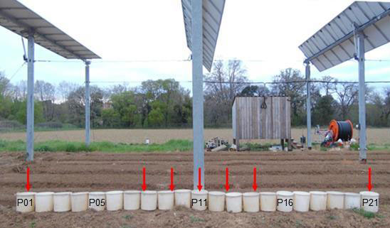
Figure 1 Effective rain and soil water content measurement under solar panels. Red arrows indicate the position of neutron probes, on a line parallel to that of the collectors, 1 m before it. Some of the P01 to P21 collectors have been identified on the picture for clarity.

Soil water content is measured with neutron probes (503DR Hydroprobe, CPN International) until 1 m depth. The soil is predominantly silty and deep. Seven neutron probes were installed at 0.0, 0.5, 1.0 and 3.2 m on both sides of the axis of rotation of the PV row (Fig. 1). Measurements are made once or twice a week on a regular basis but systematically before and after the events.

2.1.3 Experiments in controlled conditions

A reduced-size agrivoltaic device was built to characterize the influence of the tilting angle of the panels in indoor conditions, monitoring the collected rain amounts in the absence of wind with a focus on the lateral redistribution on the width of the panels (Fig. 2). The experimental device consisted of a 2 m×1 m panel on a supporting structure of reduced height, allowing tilting angles between 0 and 70^∘. A rainfall simulator composed of numerous fogging sprays was placed 1.8 m above the flat position of the panel, ensuring quasi-uniform rain conditions on the whole area of the panel, with tested intensities of 20, 35, 60 and 70 mm h⁻¹ selected to be representative of the local rain intensities (corresponding to 1-, 3-, 16- and 32-year return periods, respectively). Water flowing out of the panel was collected on a tilted plane on which 10 half-cylinders were fixed, pouring water in the corresponding 10 joined collectors of 0.1 m diameter, covering the width of the panel. The collected amounts were weighted at the end of each test and converted into water depths.

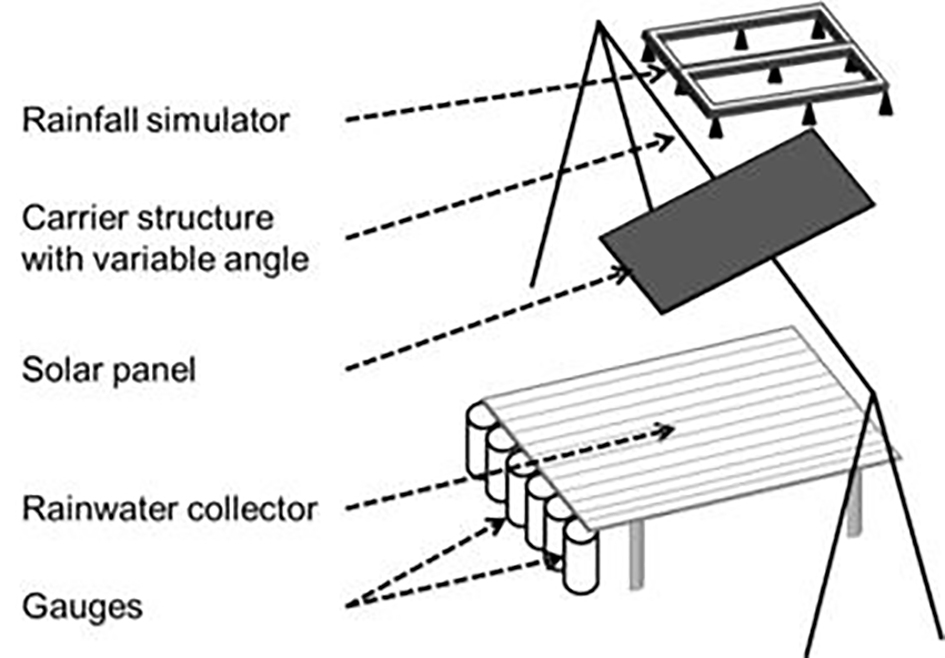
Figure 2 Experimental device used for indoor tests, focusing on lateral rain redistribution on the width of the panel, for various combinations of rain intensities and tilting angles of the panel.

2.2 Rain redistribution model (AVrain)

2.2.1 Model rationale

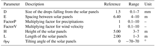
The modelling of rain redistribution by solar panels is a geometrical problem describing rain interception by an impervious surface of length L, tilting angle α_PV and height h above the ground, in which α_R is the angle of incidence of rainfall with respect to the vertical axis and θ_R denotes the plane in which the rain falls, with respect to the north in the present case (Fig. 3). The solution is studied in the vertical (x, z) plane so that the effects in the y direction will be discussed and evaluated but not explicitly described here. Finally, E is the spacing between the supporting pillars, allowing the estimation of an equivalent 1D surface coverage and thus the extension of local calculations to the whole agrivoltaic plot.

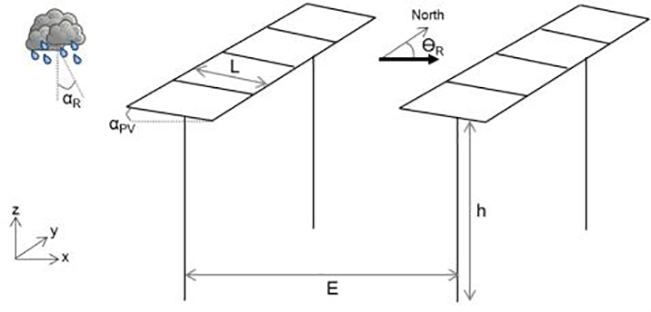
Figure 3 Scheme of the simulated scene, indicating the key parameters of the AVrain model that describes rain redistribution by the solar panels on agrivoltaic plots.

The angle of incidence (α_R in degree) of rainfall with respect to z may be estimated from the ratio between wind velocity (v_w in m s⁻¹) and the velocity of the falling rain drops (v_d in m s⁻¹), according to Van Hamme (1992).

$$\begin{array}{}\text{(1)}& {\displaystyle }\tan \left({\mathit{\alpha }}_R\right)={\displaystyle \frac{v_w}{v_d}}\end{array}$$

In the above equation, v_d is drawn from the equation proposed by Gunn and Kinzer (1949) for the free-fall limit velocity of a rain drop in stagnant air, from measurements obtained with the electrical method, which is relevant for drop diameters between 0.1 and 5.7 mm:

$$\begin{array}{}\text{(2)}& {\displaystyle }{v}_d^{\mathrm{2}}={\displaystyle \frac{\mathrm{4}}{\mathrm{3}}}{\displaystyle \frac{gD\left({\mathit{\rho }}_s-\mathit{\rho }\right)}{\mathit{\rho }c}},\end{array}$$

where g is the acceleration of gravity (m s⁻²), ρ_s is water density (kg m⁻³), ρ is air density (kg m⁻³), D is the drop diameter (m) and c is the drag coefficient (–).

Drop size distribution has been linked to rain intensity (I in mm h⁻¹) by Best (1950) from previous literature elements and measurements made by the author:

$$\begin{array}{}\text{(3)}& {\displaystyle }\mathrm{1}-F_{\text{cum}}=\exp \left(-{\left({\displaystyle \frac{D/\mathrm{1000}}{\mathrm{1.3}{I}^{\mathrm{0.232}}}}\right)}^{\mathrm{2.25}}\right),\end{array}$$

where F_cum is the fraction of liquid water in the air comprised in drops with diameters less than D.

The determination of the angle of incidence of rainfall (α_R, ^∘) from given rain intensity (I) and wind velocity (v_w) allows then

• the discrimination of the zones impacted by the presence of solar panels from those that will receive the same rain amounts as in the control zone and

• the calculation of the water amount intercepted by the solar panels (I_PV, mm⁻¹) in function of I, α_PV (^∘), α_R (^∘), θ_PV (^∘ N) and θ_R (^∘ N), after Van Hamme (1992):

$$\begin{array}{}\text{(4)}& {\displaystyle }{I}_{\text{PV}}=I\left(\cos {\mathit{\alpha }}_{\text{PV}}-\tan {\mathit{\alpha }}_R\sin {\mathit{\alpha }}_{\text{PV}}\cos \left({\mathit{\theta }}_{\text{PV}}-{\mathit{\theta }}_R\right)\right).\end{array}$$

For simplicity, it is assumed that no significant lateral redistribution occurs on the width of the panels, resulting in no variation in the outlet flow in the transverse y direction. The relevance of this hypothesis is justified in the following: the tests in indoor conditions were designed to address this issue. It is also assumed that the wetting phase of the panels before runoff initiation (somehow the storage capacity of the panels) has no noticeable effects on the calculations. From observations, for low tilting angles, the I_PV value needed to trigger runoff is 0.2 mm at most, which is a small value compared to the other values involved in the analysis (and lower than the usual precision of rain gauges).

Runoff velocity (V, m s⁻¹) is calculated with the Manning–Strickler formula, hypothesizing that flow width is much larger than flow depth, which makes flow depth approximately equal to the hydraulic radius. Manning's n coefficient is assumed to be 0.01 $\mathrm{s}{\mathrm{m}}^{-\mathrm{1}/\mathrm{3}}$ after (Chow, 1959) because of the very smooth glass coating of solar panels.

The parabolic trajectory of the drops falling from the panels is calculated in similar ways for any drop size (i.e. diameter D) and characterized by the abscissa at which the free-falling drop touches ground (x^∗, m) and the free-fall duration (t^∗, s):

$$\begin{array}{}\text{(5)}& {\displaystyle }\left\{\begin{array}{l}{x}^{\ast }=a_x{\displaystyle \frac{t^{\ast \mathrm{2}}}{\mathrm{2}}}+V\cos {\mathit{\alpha }}_{\text{PV}}{t}^{\ast }+x_{\mathrm{0}}\\ a_x=\mathrm{2}\cdot {\mathrm{10}}^{-\mathrm{4}}{\displaystyle \frac{v_w^{\mathrm{2}}}{D/\mathrm{2}}}\\ t^{\ast }={\displaystyle \frac{V\sin {\mathit{\alpha }}_{\text{PV}}+\sqrt{{\left(V\sin {\mathit{\alpha }}_{\text{PV}}\right)}^{\mathrm{2}}+\mathrm{2}g{z}_{\mathrm{0}}}}{g}},\end{array}\right.\end{array}$$

where a_x is the acceleration (m s⁻²) due to wind in the x direction, considering a drag coefficient of c≈0.5 for the drops in the air, V is the initial velocity of the fall (m s⁻¹) and x₀ is the abscissa of the edge of the PV (m).

Drop diameter measurements (expressed further in mm for convenience) were conducted with a dual-beam spectro-pluviometer (Delahaye et al., 2006). A three-mode distribution of drop diameters was revealed with peaks at D=1.4, 3.8 and 9.3 mm (Fig. 4). However, diameters D>7.5 mm might be artifacts because rain drops this size would become unstable and split in two droplets during their fall (Niu et al., 2010). In the following numerical applications, a fixed diameter of D=1.5 mm is selected as the reference case for simplicity. However, the sensitivity of the model to D is low and will be discussed later.

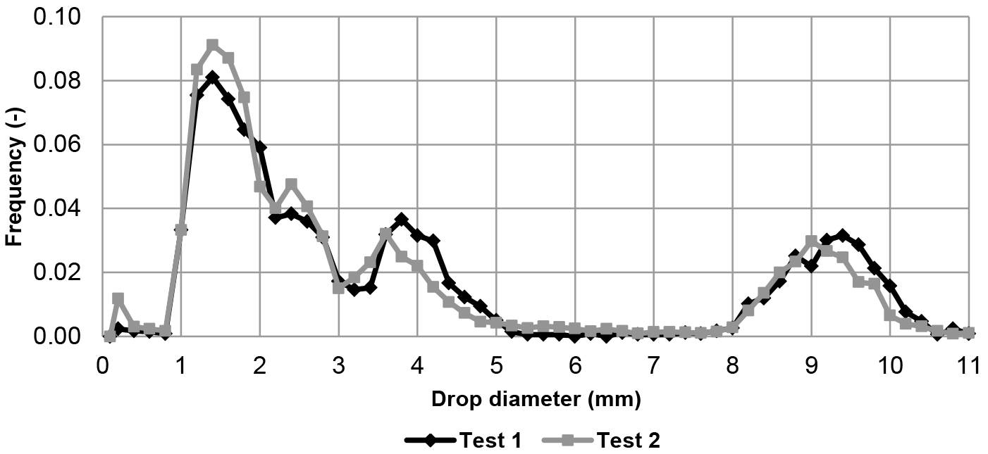
Figure 4 Drop-size distribution curve, obtained with a dual-beam spectro-pluviometer, for the drops falling from the edge of the solar panels. The frequency plotted on the y axis indicates the count of diameters D observed with respect to the total count (the step is about 0.2 mm for D).

The AVrain model was developed with the R software to describe 2D (x, z) phenomena in the vertical plane, hypothesizing negligible effects in the transverse (y) direction (Fig. 1). The time step of AVrain is 1 min. The required climatic forcings are rain intensity (I), wind velocity (v_w) and direction (θ_R), which is assumed identical to rain direction. The input parameters are the geometrical descriptors of the structure: the height of (the axis of rotation) of the panel (h), its length (L), tilting angle (α_PV) and orientation (θ_PV), plus the spacing between (pillars supporting the) solar panels (E). Only the tilting angle can be a function of time as it denotes the control exerted on the system. AVrain allows calculating rain redistribution (in x) in the form of effective cumulative rainfall amounts as a function of time. A known limitation of this simplified model is that the effects of the secondary slopes of the panels are not explicitly accounted for, although they are properly identified by the experiments in controlled conditions. These have shown that the combination of low tilting angles (i.e. primary slopes α_PV<5^∘) and low rain intensities lead to lateral dispersion on the edge of the panels. In these cases, this leads to concentrated water fluxes on the lower corner of the panel. However, the impact on the water balance (and its heterogeneity) is limited due to the low magnitude of the corresponding rainfall amounts, as discussed in Sect. 4.1.

2.2.2 Sensitivity analysis

The implementation of solar panels is very likely to affect crop management and irrigation strategies in the equipped plots, especially because of rain redistribution by the panels. The associated patterns of spatial heterogeneity may be described by the coefficient of variation (Cv) closely related to the coefficient that describes the uniformity of water distribution by the irrigation systems (ASAE, 1996; Burt et al., 1997), thus allowing easy comparisons. The choice of Cv as the target variable for sensitivity analysis acknowledges spatial heterogeneity is the key descriptor of the effects of solar panels on rain redistribution on the cultivated plots. In the following, Cv is calculated from the effective rain amounts (i.e. the cumulative water depths) simulated in the 21 joined collectors along the x axis. High Cv values indicate strong heterogeneities while values below 0.2 will be considered as acceptable, according to the standards of ASAE (1996) for irrigation uniformity. This threshold of 0.2 is also consistent with the reference values reported in Van der Gulik et al. (2014).

Using Cv as an indicator allows accounting for two sources of spatial heterogeneity: rain redistribution by the solar panels (with eventual local effective rain amounts that exceed the natural rain amounts measured in the control zone) and the sheltering effect of solar panels (with effective rain amounts far lower right under the panels than in the control zone). In more detail, Cv encompasses in a single indicator the spatial heterogeneity observed within the region located right under a solar panel, i.e. centred on the transverse y axis that connects two supporting pillars, as clearly seen in Fig. 1 where the P11 is the central collector. The width of the equipped region is E, selected as the parameter that describes the spacing between panels and further used to estimate the 1D spatial coverage of the plot by the panels, also taking place in the sensitivity analysis of the model.

The Morris (1991) method is used with Cv as the target variable to estimate the sensitivity of the AVrain model to assess the effect of its seven main parameters (see Table 1) on the spatial heterogeneity of rain redistribution by the solar panels. The combined one-at-a-time screenings of the parameter space introduced by Campolongo et al. (2007) have been used to cover a wide set of possible agrivoltaic installations, keeping all parameters within acceptable, realistic ranges of values. The “sensitivity” package of R (Pujol et al., 2017) was used to generate the associated 4000 parameter sets, obtained from p=7 parameters with d=500 draws each, dispatched within r=8 levels. The control parameter (tilting angle θ_PV of the panels) was taken between −70 and +70^∘ but held fixed for the tested event (P=3.6 mm, v_w=0.78 m s⁻¹, θ_w=285^∘, described later).

Table 1 Parameters and ranges of values used in the sensitivity analysis of the AVrain model.

2.3 Control simulations of soil moisture field by Hydrus-2D

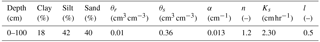
Hydrus-2D (Simunek et al., 1999) may be used to simulate water redistribution in soils for different fixed tilting angles of the solar panel or strategies for operating the panels. The simulation domain finds itself in a vertical (x, z) plane; it is centred on the supporting pillar of a panel and covers a total width of 6.4 m, corresponding to the distance between two consecutive pillars. Hydrus-2D is instead used here for coherence checks and to gain an overview of water redistribution in soil than for detailed numerical simulations of the wetting front movements in space and time, thus allowing simplifying hypotheses on soil structure. The investigated soil depth is 1 m deep, well known from numerous local experiments, and predominantly silty. It is assumed homogeneous in the absence of significant contrast with depth and presented in Table 2.

Table 2 Soil parameters at the Lavalette experimental station used in Hydrus-2D. θ_r and θ_s denote, respectively, the residual and saturated volumetric soil water contents, α and n are empirical shape parameters of the Van Genuchten–Mualem model, K_s is the soil hydraulic conductivity at saturation and l is a pore connectivity parameter.

The AVrain model provides the time-variable forcing data at the soil–atmosphere interface for Hydrus-2D, divided into five categories and accounting for time-variable tilting angles of the solar panel (Fig. 5):

• atmospheric conditions for zones not impacted by the presence of the solar panel,

• flux 1 (F1) conditions for zones impacted by the panel and located right under it,

• flux 2 (F2) conditions for zones impacted by the panel but not located under it,

• flux 3 (F3) conditions for zones located under the edge of the panel thus exposed to the largest effective rain amounts and

• flux 4 (F4) conditions for zones adjacent to those of the F3 conditions but on the sheltered side.

Hydrus-2D currently allows five types of time-variable upper boundary conditions, which suggests using F2 on both sides of the panel, as indicated in Fig. 5 where only the leftmost position of F2 corresponds to the choices listed above. However, the rightmost position of F2 seems the most suitable default choice given the known soil filling dynamics and the expected effective rain amounts. Zero-flux boundary conditions apply on the vertical limits of the domain and free drainage is relevant for a bottom boundary condition because the water table is several metres under the limit of the domain. For simplicity, the initial soil water content will be assumed homogeneous, selecting a value close to the available observations (θ=0.15).

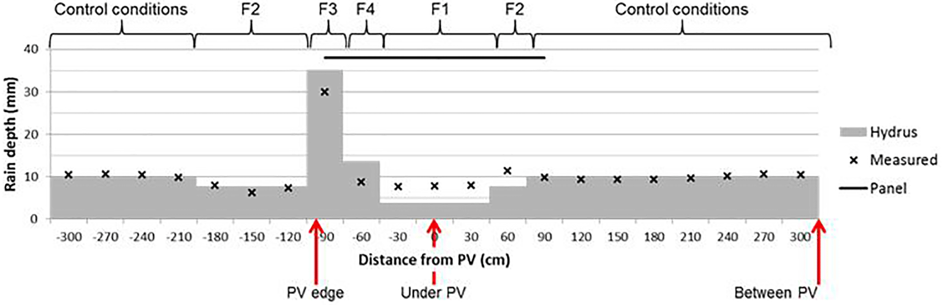
Figure 5 Time-variable upper boundary conditions used in Hydrus-2D for the tested rain event, during which the tilting angle of the panels was varied to minimize rain interception (avoidance strategy).

3 Results

3.1 Rain redistribution measurements on the dynamic agrivoltaic plot

The influence of variable-tilting-angle solar panels on rain redistribution was measured thanks to a wide series of rain events covering a full year. For each event, we put a focus on the spatial heterogeneity, which is assumed to be a crucial issue for the hydrological balance of solar panels on crops. This heterogeneity is characterized with the coefficient of variation Cv of rain depths. Table 3 gathers Cv values obtained for the most documented rain events in the available records. It enables comparisons between Cv and the tilting angle (or operating strategy) of the solar panels for various rain intensities. The least heterogeneous rain redistributions were observed for panels in abutment (Fig. 6a and b) mainly due to decreased surface coverage, from 30 % for flat panels to 20 % for panels in abutment, resulting in a lesser rain interception. However, the relevancy of this strategy depends on the angle of the wind with respect to the panels (α_R vs. θ_R) identifying these as second-order but non-negligible factors, according to which Cv may become twice as large for panels “facing the wind” or “back to the wind”. By contrast, the most heterogeneous rain redistribution was observed for a flat panel (α_PV=0) maximizing rain interception and concentration by the panel (Fig. 6c), collecting 11 times more rain than in the control zone, in the F4 domain of Fig. 5, with Cv =2.13.

Strategies involving time-variable tilting angles α_PV offer multiple possibilities, among which the previously mentioned avoidance strategy is relevant to decreasing the spatial heterogeneity (Fig. 6d) and results in Cv =0.22, which is a fairly good homogeneity. For all the events listed in Table 3, only the avoidance strategy was able to provide an acceptable level of uniformity in the agrivoltaic plot, i.e. a spatial heterogeneity then would not need to be corrected on purpose, with a dedicated precision irrigation device to ensure equivalent water availability conditions during crop growth. In all cases, the effective rain depth was more important on the sides of the panel (collectors 9 and 13 in Figs. 1 and 6). There are non-impacted zones in the free space between panels, where the effective rain is the same as in the control zone. On the contrary, the sheltering effect is strong right under the panels and the effective rain is always far lower than in natural conditions.

Table 3 Rain events with their identification (ID), date, rain amounts on the control zone (P0), tilting angle of the solar panels (α_PV) and the associated measured coefficient of variation (Cv) whose highest values indicate the strongest spatial heterogeneities in rain redistribution by the solar panels. In the “Comments” column, avoidance strategy indicates a time-variable α_PV angle to minimize rain interception by the panels in real time.

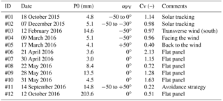
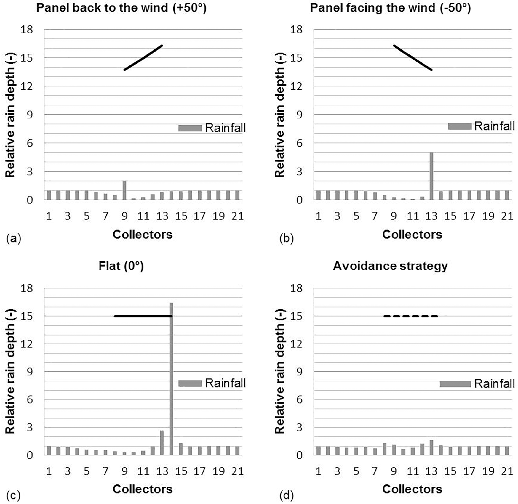
Figure 6 Examples of rain redistribution for various rain events, tilting angle and operating strategies of the solar panels, measured in the collectors displayed in Fig. 1. Relative rain depths are given with respect to the control zone where rain amounts are collected in the pluviometer.

3.2 Evaluation and sensitivity analysis of the AVrain model

The rain redistribution model AVrain was tested for 11 rain events involving flat panels, panels in abutment (either back to the wind or facing the wind) and avoidance strategies, as presented in Table 4. AVrain describes rain redistribution with a satisfying mean determination coefficient of R²=0.88. The values of MAPE (mean absolute percentage error) mostly were between 0.1 and 0.3, and regression coefficients greater than 1 indicate that the model tends to overestimate the real effective rain amounts. However, Fig. 7 shows that the overestimations occur near the drip line (i.e. the aplomb, which is used in its technical sense to designate the point on the ground located exactly under the edge of the panel) of the panels, totalizing about 25 % of the committed errors.

Table 4 Performances of the AVrain model that describes rain redistribution by the solar panels, identifying each event (ID), indicating the mean absolute percentage error (MAPE), normalized root mean square error (NRMSE), linear correlation coefficient and coefficient of determination (R²) next to the simulated coefficients of variation (Cv). The highest Cv values signal the strongest spatial heterogeneities in rain redistribution by the solar panels.

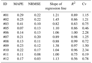
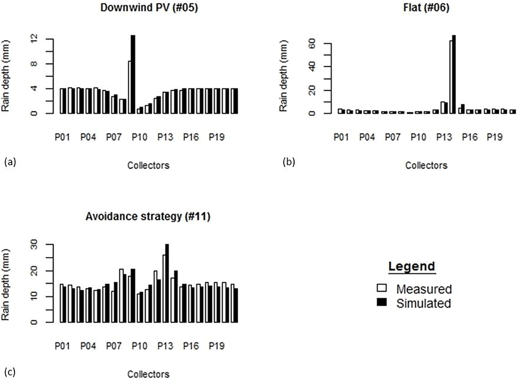
Figure 7 Examples of rain redistribution by the solar panels simulated by the AVrain model and compared to field measurements for three very different events and managements of the solar panels (see Tables 3 and 4 for details).

The sensitivity analysis of AVrain was conducted with the Morris (1991) method modified and improved by Campolong et al. (2007), selecting Cv as the target variable. Figure 8 shows its results, where µ^∗ on the x axis is the mean of the individual elementary effects (thus the sensitivity of the parameter tested alone) and σ on the y axis represents the SD of the elementary effects (thus the sensitivity of the parameter tested in interaction with other parameters). The Morris plot allows identifying the parameters that have (i) a negligible overall effect, denoted by low values of both µ^∗ and σ; (ii) a linear effect, denoted by high values of µ^∗; or (iii) non-linear or interactive effects, denoted by high values of σ. The sensitivity measures (µ^∗, σ) reported in Fig. 8 for each parameter have been normalized by the value of the highest sensitivity measure (σ) for the most sensitive parameter (FactorV).

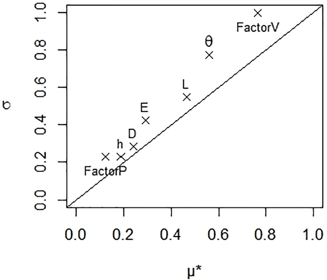
Figure 8 Sensitivity analysis of the AVrain model by the Morris (1991) method improved by Campolongo et al. (2007), where µ^∗ indicates the linear part of the total sensitivity score for each parameter while σ indicates the non-linear or interactive part. In the Morris plot, D is the drop diameter, E the spacing between solar panels, FactorP is the multiplying factor for precipitations with respect to the reference case, FactorV is the multiplying factor for wind velocity with respect to the reference case, h is the height of the solar panels, L is their length and θ_PV is their tilting angle (see Table 1 for the reference values and ranges of the parameters). The target variable of the analysis was the coefficient of variation that measures the spatial heterogeneity of rain redistribution by the solar panels. The tested rain event was #06 in Tables 3 and 4.

The position of the parameters above the 1:1 line in Fig. 8 signals that AVrain is more sensitive to the interactions between parameters than to individual variations in the parameter values, which reinforces the fact that strong heterogeneities in effective rain amounts most likely occur when several conditions are met at once in the forcings (wind direction, drop size), the controls (tilting angle) and the structure (fixed characteristics of the panels). In particular, the high sensitivity score of FactorV compared to the low score of FactorP indicates that wind velocity tends to influence rain redistribution patterns far more than rain amounts, likely because wind velocity intervenes in the calculation of the angle of incidence of rainfall and in that of the trajectory of the drops falling from the panels. The drop size itself was found to have a non-negligible but rather weak influence, although a wide range (0.1 to 7.0 mm) of values was tested. The fact that AVrain is more sensitive to the tilting angle (control exerted on the system) than to the structure parameters (fixed once selected during the installation) is a crucial result of the analysis, indicating there is room for optimization. Conversely, the higher sensitivity of AVrain to wind velocity than to the tilting angle confirms that the optimization strategies should be decided from wind characteristics that dictate the angle of incidence of rainfall.

Figure 9 Graph showing the influence of the structure parameters (spacing E, height h, length L) of the agrivoltaic installation on the spatial heterogeneity of rain redistribution by the solar panels, from the simulated values of the coefficient of variation (Cv).

In an overview of Fig. 8, the Morris method unveils the hierarchy of effects. This proves especially useful when investigating the interactions between the structure parameters. For example, the combinations between panel length and spacing (defining surface coverage) are expected to have more effect on the target variable than the combinations involving panel height, making height a second-order parameter, at least for the tested (realistic) ranges of values and the chosen target variable. This conclusion would have been impossible to reach when separately testing the effects of variations in length, spacing and height of the panels, as proven by Fig. 9, which only acknowledges adverse effects (on Cv) of length and spacing on one side and of height on the other side.

From Fig. 8, the influence of the tilting angle may be expected to be larger than that of the structure parameters, anticipating thus that the avoidance strategy (i.e. operating the panels so as to minimize rain interception) will be likely to significantly reduce Cv whatever the structure parameters. This point is further investigated by Fig. 10, comparing a flat panel with a piloting of the panel according to the avoidance strategy, for various combinations of panels length and spacing (previously proven to have more influence on Cv than the height of the panels). Small-sized panels with a low spacing between them is advocated as the best configuration to reduce Cv in avoidance strategies, which is simulated to be far more efficient than panel held flat. However, this analysis indicates the direction to follow when only rain redistribution issues are tackled but external constraints will surely exist when deciding the in situ implementation of such agrivoltaic installations, for example in the form of limit values for the spacing between panels (to allow agricultural activities).

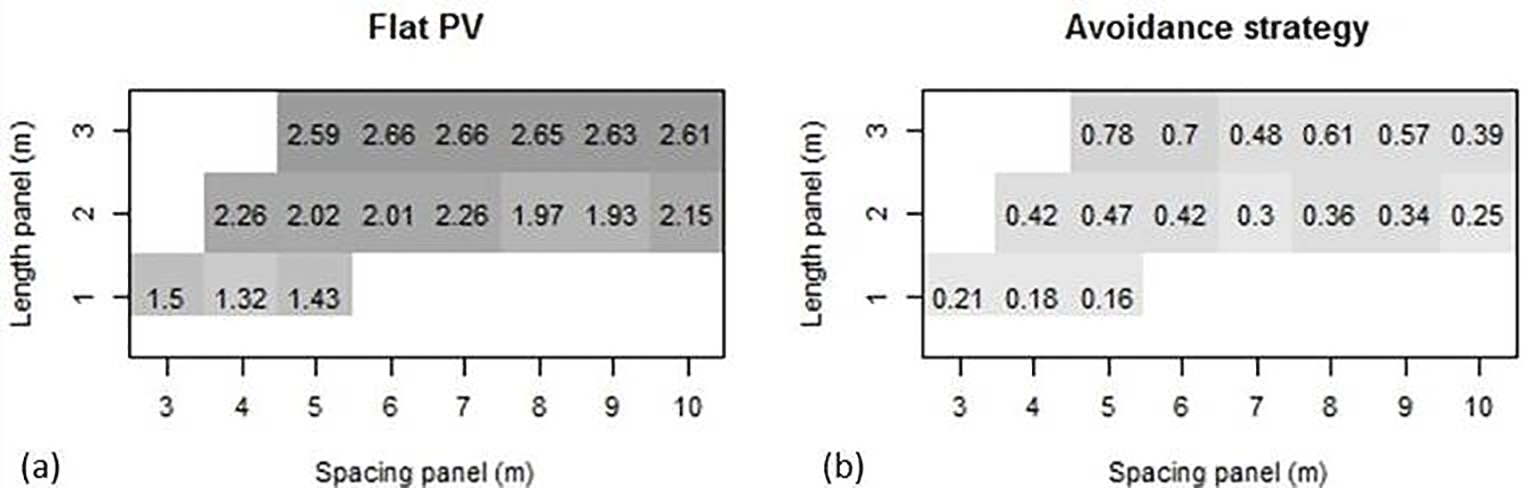
Figure 10 Influence of the structure parameters (spacing E, length L) of the panels on the spatial heterogeneity of rain redistribution from the simulated values of the coefficient of variation (Cv) for panels held flat (a) or operated according to the avoidance strategy (b). The combinations of E and L values may be assimilated to equivalent 1D surface coverage between 20 and 60 % by dividing L by E. Only the realistic combinations have been simulated here: blank cells indicate those that are not.

3.3 Rain redistribution in soils

Water content profiles were measured in the agrivoltaic plot immediately before one of the rain events, and then 6 to 12 h after it, to identify the dynamics and magnitude of rain redistribution in soils, as a consequence of rain redistribution on the soil surface. As expected, the spatial heterogeneity observed on the soil surface is transferred but becomes a bit fuzzy in the first 30 cm of soil, due to lateral homogenization (ponding with significant surface runoff, lateral diffusion associated with soil dispersivity). Nevertheless, the spatial patterns are clearly visible within soils, especially for the flat panels case (Fig. 11a) for which three distinct zones may be identified: (i) between panels, with similar behaviour as in the control zone; (ii) under panels, with a noticeable sheltering effect and thus drier soils; and (iii) under the edge of the panels, where the increased soil water content is attributable to the large effective amounts poured on the soil surface. In Fig. 11a, the maximal soil water storage variation was observed under the edge of the panels, estimated at 6.7 mm in accordance with the location of the effective rain amount poured on the soil surface (24.0 mm). Between panels, the storage variation was 2.0 mm for 3.0 mm of effective rain. Under panels, the storage variation was 4.7 mm for only 1.3 mm of effective rain, which reinforces the hypothesis of lateral redistribution, either within the soil or at its surface, from the nearby zones. In Fig. 11b, the avoidance strategy tested for a rain event of 60 mm in the control zone resulted in a maximal storage variation of 91 mm between panels due to a drier initial soil water content, 76 mm under panels and 43 mm near the aplomb of the edge of the panels, while significant ponding was observed.

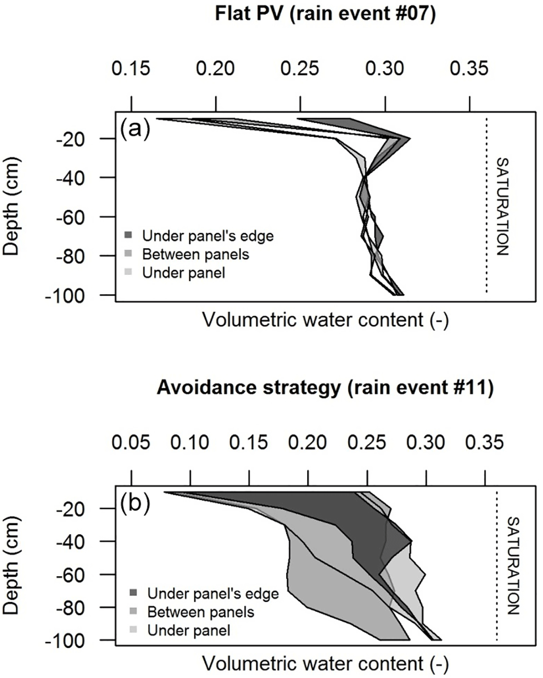
Figure 11 Variations of soil water storage in soil regions located near the aplomb of the panel's edge (dark grey), between panels (medium grey) and under panels (light grey) for different strategies for operating the panels, holding panels flat during rain event #07 (a) or operating them according to the avoidance strategy that minimizes rain interception during rain event #11 (b). For each case, the leftmost and rightmost line indicate the water content profile before and after the event, respectively. Event #11 was considered as the sum of two successive events for a total rainfall of 60 mm in the control zone.

The simulation of rain redistribution in soils was made by Hydrus-2D for a single rain event (#11) to compare the soil water content fields obtained in the flat panel case (Fig. 12a) or when using the avoidance strategy (Fig. 12b). The time-variable atmospheric conditions required by Hydrus-2D were provided by the outputs of AVrain at the minute time step, with the five-zone discretization discussed in Sect. 2.4 and shown in Fig. 5. Starting from a rather dry, realistic and approximately homogeneous soil water content of θ=0.15 cm³ cm⁻³, the objectives of these exploratory simulations were not to capture the finest spatial patterns of the wetting front, but instead to assess whether the observed noticeable differences in rain redistribution trends could easily be reproduced and quantified by Hydrus-2D. As expected, the flat panel case leads to the creation of a sharp contrast in soil water content, near the aplomb of the edge of the panel, in the form of a wet bulb that propagates downward by gravity and sideward by diffusion. This result in the vertical plane is in coherence with a well-known 3D effect of drip irrigation – that the vertical and horizontal deformations of the ellipsoidal bulb will depend on soil properties: coarse soils will produce very elongated bulbs in the vertical direction while silty soils are likely to produce more significant lateral redistribution. However, the simulated spatial heterogeneities in soil water content remain very pronounced for the flat panel case in comparison with the avoidance strategy (Fig. 12b). In this paper, the choice of the coefficient of variation (Cv) to qualify the spatial heterogeneities allowed the reconnection to the coefficient of uniformity classically used in irrigation science, addressing water delivery on the soil surface, typically by sprinkler irrigation. Here, Fig. 12a resembles the 2D or 3D patterns characteristic of surface or subsurface drip irrigation while Fig. 12b recalls the quasi-1D patterns of (high-performance) sprinkler irrigation.

3.4 Effects of the transverse slope of the panels

The underlying hypotheses made in the construction of the AVrain model led to the formulation of a 2D (x, z) model, thus discarding all phenomena arising from variations in the transverse (y) direction or, at least, not representing them in an explicit manner. If relevant, indirect assessments of their effects should still be made, outside AVrain but to investigate if the model stays valid or in which conditions significant uncertainties may exist in its predictions. Among transverse effects likely to exist in real conditions, only the effects of transverse slopes of the panels were anticipated, observed and deemed significant, though limited to particular contexts. These contexts are summed up in the cases when the tilting angle (i.e. the prevalent slope) of the panels is very low, so that the transverse, secondary slope becomes of the same order.

Tests in controlled conditions were conducted with a duration of 15 min, under a rain intensity of 20 mm h⁻¹. Rain redistribution on the width of the panel appears for tilting angles lower than 20^∘ and the width of the outlet becomes very narrow for tilting angles lower than 5^∘ (Fig. 13). In the latter case, about 90 % of the collected water drops from the panel through a 20 cm wide outlet. In the general case, such effects may be explicitly calculated from the slopes (prevalent, secondary) and water depth on the panel. Such effects are likely to increase the effective rain amounts observed in the field at the aplomb of the edge of the flat panels (Fig. 6c).

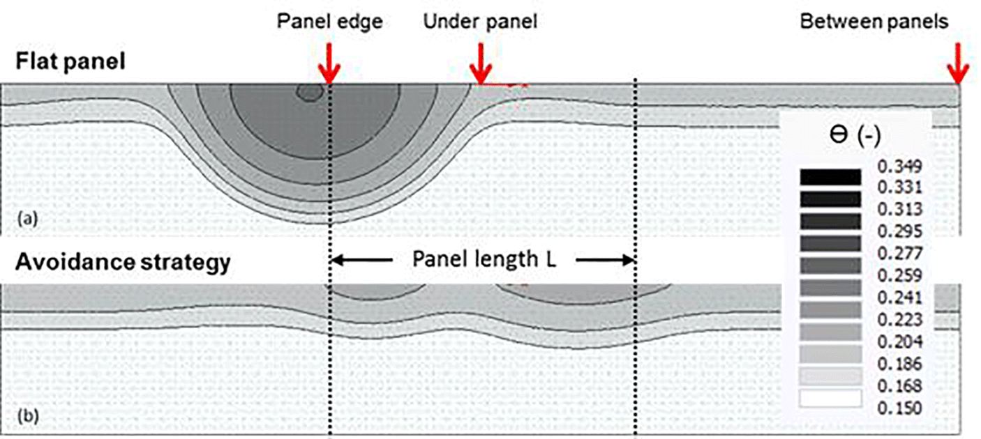
Figure 12 Simulation of soil water patterns with Hydrus-2D, in regions located near the aplomb of the panel's edge, under panels or between panels, when holding the panels flat (a) or operating them according to the avoidance strategy (b) to reduce the heterogeneity of rain redistribution by the panels during event #11 (see Tables 3 and 4). The vertical arrows recall the positions of the neutron probes used to collect water content data plotted in Fig. 11.

4 Discussion

4.1 Rain redistribution by the solar panels

The 2D AVrain model was developed to describe rain interception and redistribution by the solar panels and fulfills its objectives well: it allows the identification of the sheltered zones and of the zones in which the effective rain amounts exceed the natural rain amounts of the control zone, with a correct quantification of the associated fluxes. The angle of incidence of rainfall was found to be a key variable in the determination of the spatial patterns of heterogeneity in the effective rain amounts falling on the ground. This angle is difficult to measure but the equations derived by Gunn and Kinzer (1949) and Best (1950) allow estimating it in indirect ways.

If relevant, the AVrain model may be adapted to account for additional geometrical characteristics of the solar panels, for example to better describe the effects of the secondary (transverse) slope when it becomes of the same order as the tilting angle of the panels (i.e. their prevalent slope). This is the typical case in which the secondary slope is likely to increase the heterogeneity of rain redistribution by redistributing the collected water along the width of the panels. The presence and effect of a ridge on the length and/or width of the panels could be explicitly modelled with the techniques used in hydrology for thin flows over a weir. Even if the presence of a small ridge may affect the threshold of (approximately) 2 mm water depth thought to trigger runoff on the panels (in controlled conditions and without a ridge), it is hypothesized here that any explicit modelling would not provide a significant added value, for two reasons: the stored volumetric amounts are small when the panels are held nearly flat in the absence of rain and the avoidance strategy is recommended when rain occurs.

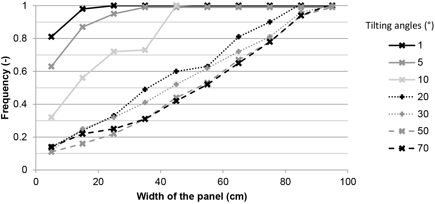
Figure 13 Influence of the transverse slope of the solar panels on the lateral rain redistribution along the width of the panel, tested for a 20 mm h⁻¹ rain intensity and “prevalent” tilting angles of the panels between 1 and 70^∘. The results are expressed in a cumulative distribution of the collected amounts at the outlets placed along the width of the panel.

4.2 Rain redistribution in soils

Hydrus-2D was used to simulate rain redistribution in soils, using the spatially distributed output variables of the AVrain model to provide the required time-variable atmospheric conditions. Five such conditions at most can be used as climatic forcings for Hydrus-2D, which seemed to be a limitation for the present purpose but could be handled, thus, with the a posteriori indication that the chosen trick has the value of a good practice. In coherence with the field observations, the simulated fields of soil water content emphasized the interest in using the avoidance strategy to decrease the spatial heterogeneities of soil water content in the agrivoltaic plots, thus confirming that the tilting angle of the panels is a strong control parameter.

Even if the spatial heterogeneity of rain redistribution is less drastic in soils than on the soil surface, due to lateral diffusion, it remains strong enough to necessitate a dedicated remediation in the form of precision irrigation, unless the avoidance strategy is used. In other words the avoidance strategy (that consists in minimizing rain interception and redistribution by commanding the appropriate time-variable tilting angle of the panels) has implications in the relevant irrigation strategy, making it less complex. This is an opening to a more global optimization problem in dealing with the various sources of heterogeneity, which will certainly be compared with the observed heterogeneities in crop yield on the agrivoltaic plots. In addition to the heterogeneities in the forcings (irrigation and rain redistribution) the modeller will surely have to also address these in soils, for example by means of geophysical methods that offer the possibility of similar spatial resolutions (e.g. electrical resistivity tomography, refraction seismology)

4.3 Rain and crop-induced operation of solar panels

Some aspects specific to cultivated plots need to be mentioned here, although the primary scope of this paper is to focus on the hydrological side. The panels left with a low tilting angle (high surface coverage and rain interception) are likely to have unwanted direct effects on the soil and plants underneath. For example, leafy vegetables might be damaged by the repeated drop impacts or even more so by the occasional curtains of water falling from the panels a few metres above, even if their storage capacity is limited. Such problems will typically occur in the morning, when panels are first operated, given that they are generally left flat during nighttime. They could also occur during heavy rains, even when using the avoidance strategy, which results in a damped but non-zero flux concentration near the aplomb of the edges of the solar panels. In the bare soil periods, it is rather the erosion risk that should be handled, especially the splash erosion (Nearing and Bradford, 1985; Josserand and Zaleski, 2003; Planchon and Mouche, 2010) where drop impacts are responsible for particle detachment and for the creation of microtopography. This, in turn, creates pathways for runoff and further soil degradation processes. Nevertheless, avoidance strategies fed by real-time wind and precipitation data (collected at a 30 s time step) are powerful means to handle these issues, which will certainly be included in the more general optimization strategies suitable for the cultivated agrivoltaic plots. In some contexts, randomized positions of the solar could be another option to reduce the consequence on soil of rain concentration and maximize homogeneity in the long term.

5 Conclusions

Agrivoltaism represents a modern, relevant solution to the growing food and energy demands associated with a global population increase, especially in the current climate change context. Nevertheless, there are unresolved issues specific to the implementation of solar panels on the cultivated plots, for example regarding the adaptation of the plants to the forced intermittent shading conditions or the impact of the panels on the hydrological budget and behaviour of the plot. This paper has tackled the pending question of rain redistribution by dynamic solar panels, i.e. panels endowed with 1 degree of freedom in rotating around their supporting axis, so that their tilting angle may vary in time and be controlled on purpose for a very short term of a few minutes.

A dramatic difference was observed and simulated, in terms of spatial patterns of rain redistribution on the ground, between the case of panels held flat and panels moved according to so-called avoidance strategies that consist in minimizing rain interception by the panels during the course of rain events (and eventually adapting the command of the panels to short-term changes in wind and rain conditions within a single event). The avoidance strategies resulted in far lower coefficients of variation (i.e. heterogeneity measures) used to describe the spatial variations in the effective rain amounts falling on the ground, under the panels, between panels or near the aplomb of the edges of the panels. The measures of heterogeneity obtained for avoidance strategies had low enough values to be compared with the fairly good uniformity scores used to quantify the ability of irrigation systems to deliver similar water amounts in the different zones of a given plot. Hence, it is likely that the most relevant irrigation strategies will suppress or attenuate the need for precision irrigation within the equipped plots. On the contrary, basic strategies that consist in holding the panels flat induce very strong spatial heterogeneities, with local effective rain amounts that exceed those of the control zone and may be responsible for increased runoff and erosion risks on bare soils, not to mention the risks associated with direct, repeated impacts on the soil aggregates (possibly leading to soil compaction and crust formation) and on the plants that find themselves near the aplomb of the edge of the panels. The flat panel case has one additional disadvantage: the panels are never strictly flat, so any transverse slope of comparable order will have the consequence of redirecting all the collected water towards a narrow outlet on the width of the panels.

However, the mechanistic AVrain model derived in this paper shows that the control exerted on the tilting angle of the panels is strong enough for the user to cope with most meteorological conditions (rain intensity, wind direction and velocity) and realistic structure characteristics (height, length and spacing of the panels) to achieve the targeted short-term event-based optimization of rain redistribution. It is very likely that more general and complex methods should be used when considering at the same time the hydrological budget, crop growth and energy production, as well as seasonal objectives. To prepare ground, the soil part of the problem has also been investigated here, showing with Hydrus-2D simulations that rain redistribution patterns in soils resembled those observed on the soil surface, though less contrasted due to lateral diffusion processes on the soil surface (ponding) or within soils (at least where significant lateral dispersion coexists with gravity). Future research leads include a finer parameterization of Hydrus-2D for a stronger coupling with the results of the AVrain model, as a verification tool for the adaptation of simpler 1D approaches to model water budget, irrigation strategies and crop growth in agrivoltaic conditions (Khaledian et al., 2009; Mailhol et al., 2011; Cheviron et al., 2016) within global optimization strategies.