River intermittency: mapping and upscaling of water occurrence using unmanned aerial vehicle, Random Forest and remote sensing landscape attributes

Although intermittent rivers exist naturally, climate change along with changes in land use and occupation have a direct influence on streamflow permanence. Measurements and modelling in non-perennial rivers are still scarce and yet, essential for prediction and understanding of water scarcity scenarios. Thus, this work aims to map and model the spatio-temporal dynamics of an intermittent river. The study area is the Umbuzeiro River in the Brazilian Semiarid (∼ 100 km), whose spatially coherent streamflow occurs exclusively in the wettest months during the rainy season. We conducted twelve UAV surveys between March and November 2022 in selected river reaches. With the imagery from UAV surveys, we classified river reaches into “Wet”, “Transition”, “Dry” or “Not Determined” with visual inspection of 1.0 m reaches. In order to explain the observed patterns, we analysed 40 candidate predictors based on static and dynamic landscape attributes and grouped them into three Random Forest models based on the different source for dynamic predictors. Among these, altitude, drainage area, distance from dams, and one different dynamic predictor per model proved to be the most informative in Random Forest models. The selected models differ in the source and type of dynamic predictor used to capture the temporal dynamics: (a) series of Sentinel MNDWI; (b) series of Planetscope NDVI; and (c) antecedent precipitation index (30 d). All model variants successfully described river intermittency with an accuracy of around 80 % for both test and training datasets. Models (a) and (b) captured the temporal dynamics in model extrapolation to the whole river. When analysing the spatial distribution of flow intermittency, models (a) and (c) better identified areas more prone to “Wet” or “Transition” classes. This way, model (a) was identified as the most successful in simulating intermittency both temporally and spatially. The use of Sentinel MNDWI in model (a) aggregates enough spatial information, so the model can better simulate water occurrence classes. The findings presented here emphasize the possibility of using this index even in narrow non-perennial rivers, although its performance may vary depending on local hydrological and environmental conditions. The modelling framework developed in this study contributes to a broader understanding of flow intermittency as a spatially complex and highly dynamic process over time. The integration of high-resolution predictors demonstrates a scalable and adaptable approach for mapping wetness conditions in non-perennial rivers using landscape attributes, dam presence, and satellite indices as predictors.

1 Introduction

The presence of intermittent and ephemeral rivers is increasingly prevalent in drainage networks around the world (Messager et al., 2021). Although they have always existed naturally, changes in land use and land cover further influence the permanence of runoff (Shanafield et al., 2021). According to recent research, changes in temperature, precipitation, damming structures, and human water demands can increase the irregularity of spatio-temporal characteristics in rivers and make them more intermittent (Messager et al., 2021). Additionally, regions already prone to flow cessation are likely to present an amplification of drying, expressed as increase in drying extent and duration under climate change scenarios (Reynolds et al., 2015; Sauquet et al., 2021).

In semi-arid regions there is a prevalence of intermittent rivers. Surface runoff is largely controlled by low annual precipitation and intense but short rainfall events (De Figueiredo et al., 2016). Furthermore, high evapotranspiration rates influence watercourses in these climate zones (Pereira et al., 2019; Costa et al., 2021; Rodrigues et al., 2021). It is of vital importance to study naturally occurring intermittent rivers due to their impact in local and regional water availability, socio-hydrological relations, biodiversity, and ecological functions and services (Medeiros and Sivapalan, 2020; Fovet et al., 2021; Pereira et al., 2025).

Intermittent rivers are non-perennial rivers or streams with variable cycles of wetting and flow cessation, with surface flow sustained for periods longer than individual storm events and influenced by groundwater contributions (Busch et al., 2020). In addition to this temporal discontinuity, flow intermittency interrupts hydrological connectivity along the river and produces spatial discontinuity as well. This happens both by the formation of disconnected river reaches and the contraction of the entire network (Godsey and Kirchner, 2014; van Meerveld et al., 2019; Prancevic et al., 2025).

The temporal and spatial discontinuity of stream flow strongly affects the patterns of physical, chemical, and ecological processes (Costigan et al., 2016; Shanafield et al., 2021). An example is the assessment of the ecological status of intermittent rivers that depends on the duration of the drying phase (Mazor et al., 2014). In addition, metacommunity assembly mechanisms can have a seasonal response to changes in hydrological conditions of intermittent rivers (Sarremejane et al., 2017). The evaluation of spatio-temporal patterns of water occurrence throughout the river is also important for studies on water supply to diffuse populations, global changes, and extreme events (Jaeger et al., 2023; Mimeau et al., 2024).

The drying and re-wetting cycles create complex hydrological patterns of diverse water occurrence patches. Extrapolating point data from fluviometric stations is not enough to characterize the spatio-temporal variation of these patterns throughout a drainage network (Snelder et al., 2013; Costigan et al., 2017; Beaufort et al., 2019; Mimeau et al., 2024). Usually, fluviometric measurements record the characteristics of only one transect. They can be useful to study the frequency of low flow events in that part of the river network (Eris et al., 2019), but not to understand how the dry and wet patches are distributed in a reach. The wetting and drying patterns of intermittent rivers are important to quantify the amount of flowing, pooled and dry conditions which directly affects the habitats for aquatic and terrestrial species (Sefton et al., 2019). Data collection along a river reach can be used to estimate water occurrence dynamics in similar parts of the drainage network. Therefore, it is necessary to investigate ways to collect and extrapolate available measurements in space and time, particularly for unmonitored areas.

Unmanned aerial vehicles (UAVs) represent an accurate approach to study water resources on a detailed scale (Acharya et al., 2021) and have already been used as a tool to observe water surface areas and river stages (Niedzielski et al., 2016; Simplício et al., 2021). The high spatial resolution of most UAV-acquired images makes it possible to detect even small changes in water surface areas. For intermittent rivers, this is important because of the natural characteristics of these rivers that can be complex and very dynamic (Borg Galea et al., 2019). Water occurrence patterns can change very quickly in semi-arid climates due to very concentrated rainfall events, so through the use multi-temporal UAV surveys we can map dynamic patterns in detail.

Random Forest models have been applied to forecast the spatial distribution of drying patterns in intermittent rivers by researchers (Snelder et al., 2013; González-Ferreras and Barquín, 2017; Beaufort et al., 2019; Price et al., 2021; Mimeau et al., 2024). However, these studies usually focus on flow/non-flowing classification of river segments. It still lacks attempts to classify different spatio-temporal dynamics of water occurrence in intermittent rivers (i.e. disconnected patches). The predictors used in Random Forest models for intermittent rivers are usually related to the river physical characteristics (slope, width, drainage area, etc.) and climate variables (precipitation, temperature, etc.) (Beaufort et al., 2019; Mimeau et al., 2024). However, most of the time it is difficult to identify the main drivers of intermittency in a smaller reach and acquire suitable data. That is why the use of satellite images is being implemented in prediction models to extrapolate the observational characteristics of water occurrence in an area (González-Ferreras and Barquín, 2017; Mimeau et al., 2024).

This study addresses a critical knowledge gap on spatial patterns of intermittency in a river. Although the general role of topographic and climatic drivers is well established, little is known about how proximity to human modifications, such as farmer dams, may influence the presence of water in river reaches. Furthermore, methodological approaches capable of integrating multiple data sources (e.g., UAV, landscape attributes, and machine learning) are still limited, particularly in intermittent rivers where wet patches are hard to map.

Here, we explore how different environmental and anthropogenic variables contribute to the occurrence of water in intermittent reaches. When we combine field-based classifications with Random Forest modelling, we investigate not only the prediction accuracy of different data sources, but also the relative importance of physical attributes and land use drivers on river wetness patterns.

The aim of this work is to map and model the spatio-temporal dynamics of an intermittent river. For this, we acquire suitable field data to map different water occurrence patterns in the Brazilian semi-arid region. With Random Forest models, we model river intermittency using remote sensing-derived data and climate variables. We also identify the most important variables that affect intermittency.

2 Study area

The Umbuzeiro River is the main stream of the Benguê catchment, which comprises an area of approximately 1000 km². The Benguê Reservoir (18 hm³) is located at its outlet and was built in 2000. This catchment is located in one of the driest parts of the Brazilian semi-arid region (Fig. 1): Its mean annual potential evaporation is approximately 2500 mm and mean annual rainfall amounts to around 560 mm with high temporal variability (Medeiros and de Araújo, 2014). Vegetation is predominantly Caatinga, a dry forest that is endemic to Brazil.

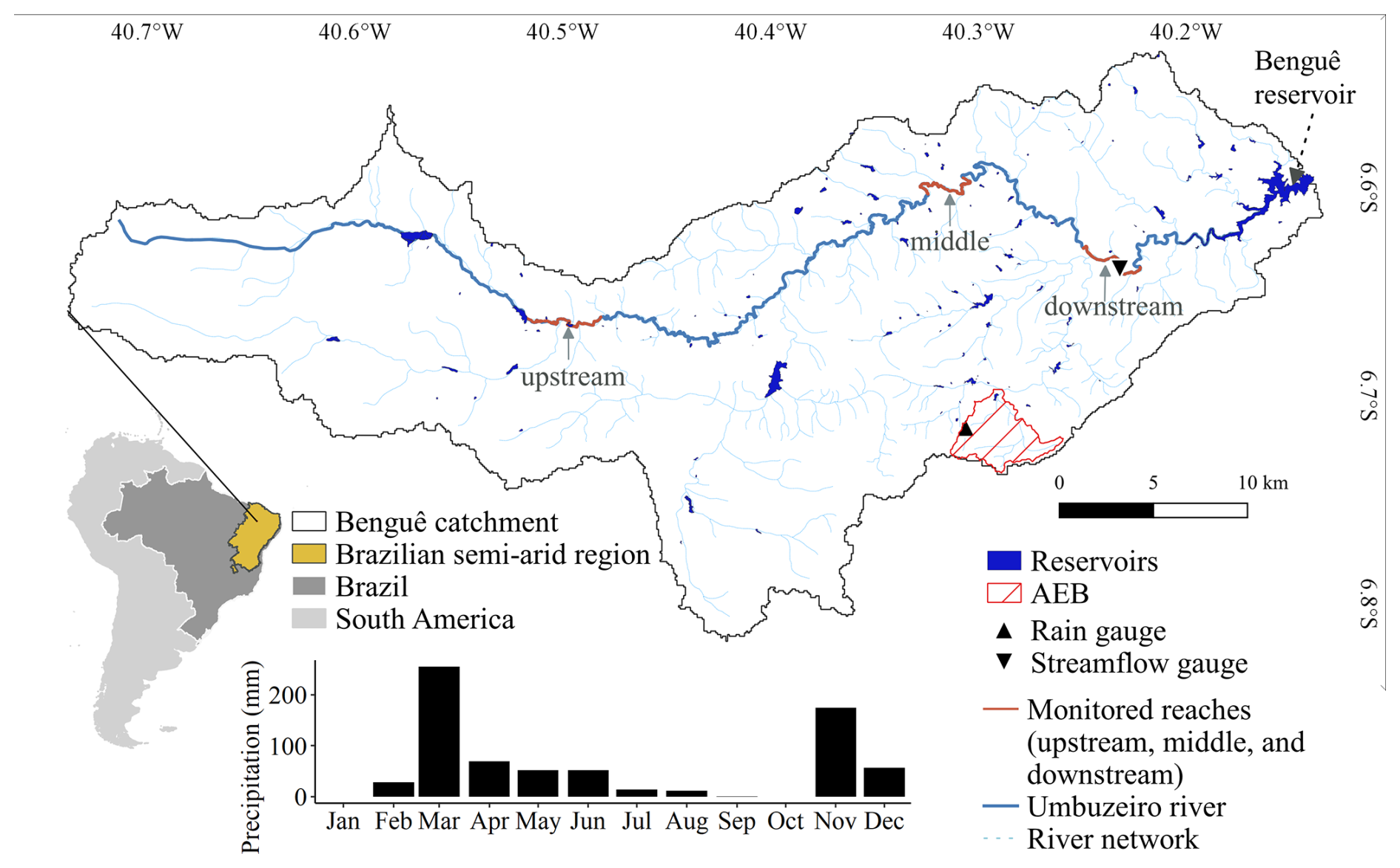
Figure 1 Umbuzeiro River in the Benguê catchment with the monitored river reaches used in UAV surveys: upstream, middle, and downstream. Precipitation is measured in the Aiuaba Experimental Basin (AEB) and it is shown the monthly data for 2022. Streamflow is measured in Aroeira section with no streamflow observed during the year of 2022.

There is a large number of reservoirs in the area, which may impact river intermittency by modifying water permanence and downstream drying patterns. According to Mamede et al. (2018), 114 reservoirs can be found in the catchment, most of them (75 %) in its lower portion. Since 2011 the streamflow has been monitored at the Aroeira section. According to measured data (2011–2020), the average streamflow occurred on 40 d yr⁻¹ with an average discharge of 0.63 m³ s⁻¹, considering only the years with any streamflow at all (7 years out of 10) (Lima et al., 2022). In Fig. 1, we can observe the three monitored reaches (upstream, middle, and downstream) and the monitoring pluviometric and fluviometric stations. The panel at the bottom of the figure illustrates the seasonal rainfall pattern, which characterizes the intermittent nature of surface water in the region.

3 Materials and methods

3.1 Modelling workflow

Workflow follows the flowchart shown in Fig. 2. There are three main steps: (1) UAV data collection and mapping, (2) model training, and (3) application to the whole river. Step 1 encompasses the river course visual mapping. Then, we conduct UAV surveys multiple times in river reaches, producing high-resolution orthomosaics. We use the images to classify 1.0 m reaches in water occurrence classes, which are used as ground-truth data for model training and evaluation. In step 2, input data from predictor variables is used during the training of Random Forest classification models in order to obtain the same class as in the observed data (UAV-derived classification). Training includes the use of static and dynamic landscape attributes as candidate predictors to explain the observed patterns of water occurrence. In a recursive process, we compute the importance of the candidate predictors (or features). We test three models based on predictor subgroups and select the most important predictors in each model. The Random Forest models are retrained with the selected predictors in order to obtain the best models. In step 3, the models are applied to the entire river. Analyses were performed using custom R scripts and datasets archived on Zenodo (Soares et al., 2026).

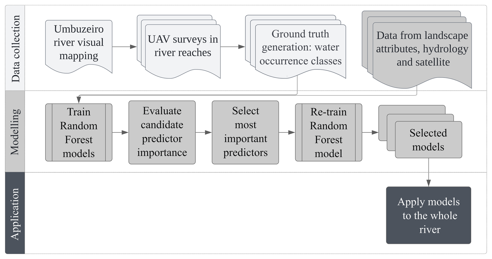
Figure 2 Flowchart display of the steps taken during the mapping and modelling of water occurrence. UAV surveys were used to generate high-resolution classification of water occurrence (1.0 m reaches), which served as ground-truth data. These classifications, alongside predictor variables, were used to train and validate random forest models of water occurrence.

3.2 Data collection

3.2.1 Modelling units

For our modelling approach, we divided the river into segments of equal size which constitute spatial modelling units (Fig. 3). Circular areas are chosen to represent these segments to better follow the river's sinuosity. The modelling units have 50 % overlap, so that adjacent conditions are considered when determining the water occurrence of each area. Analyses of stream habitats are usually measured by wetted width, where a sampling reach has a length of 20 times the maximum mean wetted width, with a recommended minimum of 50 m (Datry et al., 2021; Fencl et al., 2015). In order to make our models useful for these analyses, modelling units are also spaced every 50 m and have a diameter of 100 m.

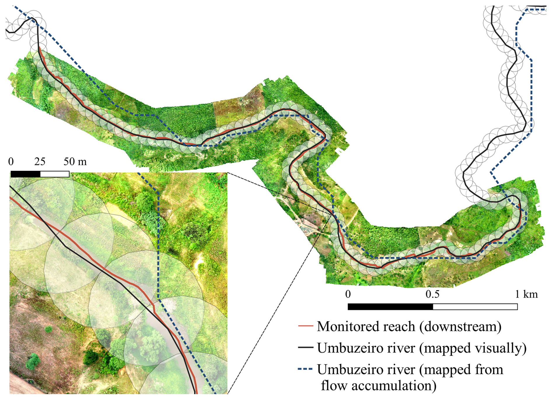
Figure 3 Difference between Umbuzeiro River mappings: the previously available mapping based on flow accumulation (from 30 m resolution DEM) versus visual mapping of the Umbuzeiro River course with satellite imagery. The average horizontal misfit between the flow accumulation path and the manually mapped stream was approximately 60 m. Image from UAV flight showing the monitored river reach. In highlight the modelling units (diameter of 100 m): river areas whose data is evaluated in water occurrence modelling.

3.2.2 Umbuzeiro River mapping

The previously available river network is derived from flow accumulation and uses a 30 m resolution DEM from the Shuttle Radar Topography Mission (SRTM) (USGS, 2009). It is relatively coarse, considering that the average width of the Umbuzeiro River is 5–15 m. There is a clear mismatch of river sinuosity when compared to drone and satellite imagery (Fig. 3). Thus, we decided to map the Umbuzeiro River course manually using Planetscope images with a resolution of approximately 3.0 m, and Google Earth Explorer to supplement information when necessary. The resulting main river branch has a length of 105 km according to this mapping (Fig. 1). The average horizontal misfit between the flow accumulation path and the manually mapped stream was approximately 60 m.

3.2.3 River reaches: data collection with UAV imagery

We acquire data in three reaches of the Umbuzeiro River. Monitored reaches were selected to capture the spatial variability across the study area, including gradients drainage areas and elevations. Therefore, reaches were distributed across the Umbuzeiro River to represent both upstream and downstream conditions. As such, the monitored reaches are considered representative of the dominant intermittency patterns within the study area.

Data acquisition occurred at different dates with two UAV systems: the copter-system Phantom 4 pro (DJI Ltd., China) and the glider-system eBee SQ (senseFly SA, Switzerland). The equipment is employed alternately depending on availability and survey requirements. The eBee SQ is equipped with multispectral cameras, and the Phantom with an RGB camera. Flight altitude varies from 160 to 190 m, ground resolution from 3.5 to 4.5 cm, and flight duration from 45 to 75 min. On average, 1000 photos are taken per flight. The coverage area varies from 2 to 4 km², and the average river reach length per flight is 5 km.

We perform UAV surveys monthly during the rainy season (April to July), and once more in November 2022 (Fig. 4). As noted by Soares et al. (2024), the rainy season typically occurs in the first half of the year in this region. The high frequency of cloud cover during the rainy season typically limits the availability of usable satellite imagery, reinforcing the need for UAV-based data collection during this period.

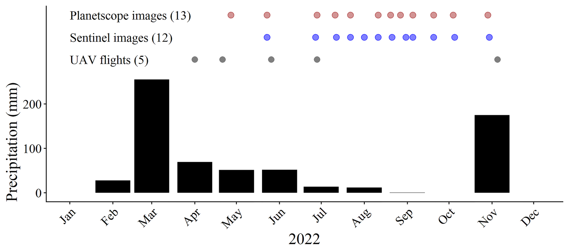
Figure 4 Monthly precipitation and dates of imagery available in 2022, indicating the number of satellite images of each sensor and UAV flights.

Images are processed in Agisoft Metashape following the default configurations recommended for each image type (i.e. multi-spectral or RGB). Processing steps include the georeferencing of flight images according to ground control points obtained with differential GPS. At the end of each processing, digital terrain models and orthomosaics are generated. Terrain models are derived from surface models created with a point cloud. With the surface model, the algorithm tries to represent the bare ground surface and builds a terrain model. The orthomosaic is generated combining the original images projected on the object surface of the terrain model (Agisoft, 2026).

The water occurrence in each monitored reach was identified with UAV-processed imagery. Classification is done in 1.0 m long reaches, which are manually assigned to one of four classes: “Wet”, “Transition”, “Dry”, or “Not Determined” (Fig. 5). The “Not Determined” class included those reaches where it was not possible to discern the riverbed, e.g. because of it being obscured by canopy. The differentiation between the other classes refers to water occurrence: “Wet” when there is water, “Dry” when there is none, and “Transition” when there seems to be water, but as it is mixed with herbaceous vegetation or algae, we cannot be sure. Usually, this occurs in transition zones between a long connected wet patch and a dry one. Since we classify 1.0 m reaches, each modelling unit has at least 100 classified reaches (Fig. 3). For modelling purposes, the most frequent class is selected for each modelling unit.

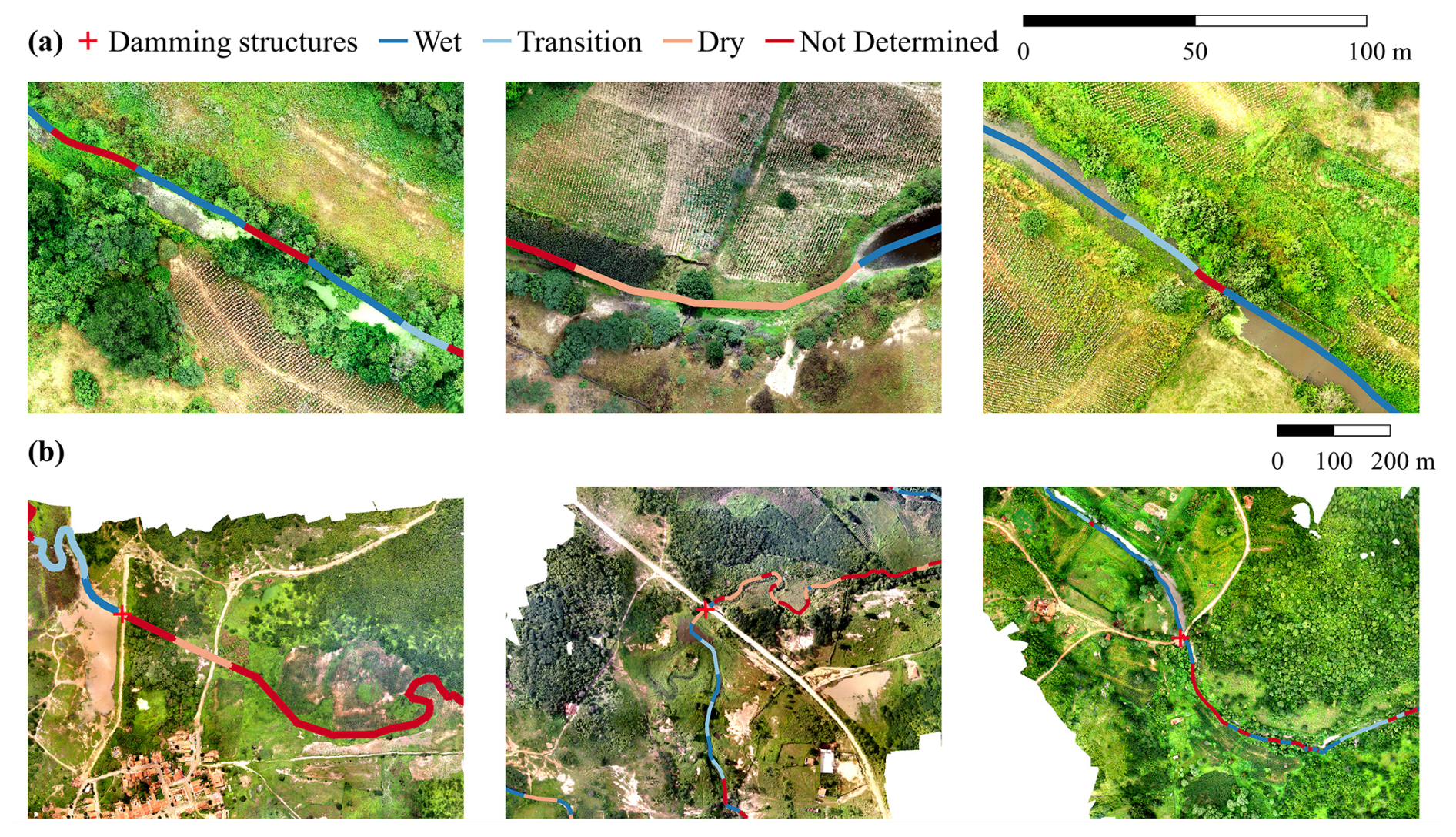
Figure 5 Examples of UAV imagery showing water occurrence classes along the Umbuzeiro River. High-resolution classification of water occurrence (1.0 m reaches) was based on visual interpretation of UAV imagery supported by field observations. We show in (a) samples of different water occurrence conditions and in (b) different examples of damming structures.

3.2.4 Spectral indices of satellite images

Input data for Random Forest training includes the use of Sentinel-2 MSI images as dynamic data. These images are freely available with a temporal resolution of five days. The spatial resolution changes according to the respective band: for the blue, green, red, and near-infrared (NIR) bands, the resolution is 10 m. For shortwave infrared (SWIR) and red-edge bands, the resolution is 20 m. The processing level is 2A after corrections and conversion of the top of atmospheric reflectance to surface reflectance. The access, processing and analyzing of sentinel images is performed in Google Earth Engine (GEE).

Planetscope images are also used as dynamic data from proprietary access. Images are available daily, under cloud-free conditions and have a spatial resolution of 3.0 to 4.1 m, the final resolution being approximately 3.0 m. The analytic surface reflectance product (level 4B) is already corrected and converted to surface reflectance. Images are downloaded from the Planet website as a “composite” (a mosaic of images available for that date). If there are missing portions, these gaps are filled with the image of the previous or following day. In thoses cases, the overlaying of different rasters (from subsequent days) is performed in R Statistical Software version 4.1 (R Core Team, 2021). Images are processed in QGIS 3.16 and R Statistical Software version 4.1 (R Core Team, 2021).

Both Sentinel and Planetscope images are used to calculate different spectral indices commonly employed for surface water detection. These indices are summarized in Table 1 and computed for all available images (Fig. 4). To use the images in the modelling process, we select images in concomitant dates (more or less one week from flight date).

Table 1 Spectral indices applied to Sentinel and Planetscope images. We present the equations for each index and the corresponding band numbers for each satellite.

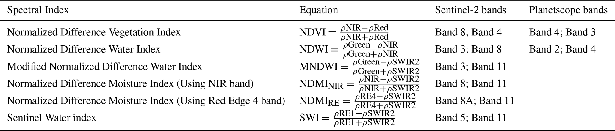
Most indices are directly related to water or moisture detection. The normalized difference water index (NDWI), modified normalized difference water index (MNDWI), and Sentinel water index (SWI) are measures to detect surface water (McFeeters, 1996; Xu, 2006; Jiang et al., 2021). The normalized difference moisture index (NDMI) is a tool to compute moisture present in leaves of vegetation, and it is calculated with either near-infrared (NDMI_NIR) or red edge bands (NDMI_RE) (Hunt and Rock, 1989; Lastovicka et al., 2020). In order to compute these indices for each modelling unit with Planescope images, the spectral indices are computed in R and zonal statistics are performed in QGIS 3.16 (QGIS Development Team, 2022) considering the mean value per area. The Sentinel indices with SWIR2 or red edge bands (20 m resolution bands) were resampled at a resolution of 10 m using nearest-neighbour interpolation. The spectral indices were processed in the GEE platform, and the mean values were obtained per modelling unit.

3.2.5 Land use and land cover

We select two land use land cover (LULC) products as input data to study their influence in the observation of water occurrence classes: Dynamic World and MapBiomas. Dynamic World is a near real-time LULC product based on Sentinel images with less than 35 % cloud cover (Brown et al., 2022). The product is delivered as new Sentinel scenes become available. Each image has a band with a discrete LULC classification, and nine probability bands featuring class-specific probability scores that are derived from the model's deep learning analysis of the spatial context of pixels (Venter et al., 2022). Dynamic World data are downloaded and processed in Google Earth Engine (GEE). For modelling purposes, we choose the discrete LULC classification for each pixel. Then, we use the major class of each modelling unit and the frequency of all classes in that area.

The MapBiomas project (https://brasil.mapbiomas.org/en/, last access: 5 November 2025) is a collaborative initiative to monitor landscape changes across Brazil's biomes. It provides annually created LULC maps with data since 1985 on the basis of Landsat images with a spatial resolution of 30 m. MapBiomas data are freely available, and we use Google Earth Engine (GEE) to access, process and analyze the data. The LULC discrete classes were processed in the platform, and the frequency of each class were obtained per modelling unit.

3.2.6 Hydrological data

We use daily hydrological data to take into account precipitation and changes in the reservoir located at the outlet of the Benguê catchment, specifically variations in water level and storage volume. During the year 2022, no streamflow is observed in the Aroeira stream gauge (Fig.  1). Accumulated precipitation data of the past 30 d is considered, and an antecedent precipitation index (API) with a k coefficient equal to 0.90 also for the respective past 30 d (Heggen, 2001).

The sensitivity of model performance to the length of the accumulation window was evaluated using periods ranging from 1 to 60 d. Model performance and predictor importance were consistent across tested windows, with no systematic improvement associated with alternative accumulation periods. Therefore, only the preceding 30 d are used, in accordance with the results of Beaufort et al. (2019) that highlighted the importance of this predictor in river intermittency modelling with Random Forest.

Regarding reservoir data, the daily water level (m) and reservoir volume (hm³) is employed, as well as variation in reservoir volume from the previous day (hm³). The Benguê Reservoir has been monitored by the Water Resources Management Company of Ceará (COGERH) since 2004.

Precipitation data are collected in Aiuaba Experimental Basin (AEB), nested into the Benguê catchment (Fig. 1). Hydrological data have been monitored since January 2003 there and precipitation data have already been considered representative for the Benguê catchment in other studies, such as the one by De Figueiredo et al. (2016). For more information on consistency of precipitation data, please see Fullhart et al. (2022). We adopt the same values of hydrologycal data for all modelling units, so there is no spatial variation of these predictors.

3.2.7 Landscape attributes

Data used to characterize landscape attributes in the modelling units are: “mean altitude”, “max drainage area”, “mean hill slope” and “number of stream cells”. We obtain them from the USGS portal (https://earthexplorer.usgs.gov/, last access: 5 November 2025) where we download SRTM DEM survey data with 30 m resolution.

Since we use SRTM data to calculate landscape attributes in each modelling unit, it is necessary to correlate both river mappings (Fig. 3). For this, the previously available flow accumulation mapping (SRTM data) is divided by the number of modelling units distributed along the visually mapped Umbuzeiro River (see Fig. 3). The river from flow accumulation is slightly shorter than the visually mapped, since resolution is finer, so modelling unit spacing in the former is shorter (44 m). We consider the same area of influence for a modelling unit (diameter of 100 m). Having the same number of units, the data are sequentially related to the visually mapped Umbuzeiro River used in the model. With zonal statistics we calculate candidate predictors per modelling unit. The number of stream cells consists in the sum of cells that were classified as river in the flow accumulation algorithm.

3.2.8 Connectivity: damming structures and water surface in reservoirs

Damming structures are mapped all along the Umbuzeiro River by using Planetscope images so as to visually locate each dam (Fig. 5b). This mapping also takes into consideration previous knowledge and field observations about the presence and location of damming structures on the river, including barrages for water storage and smaller farm dams. In total, 45 of this kind of structures in the Umbuzeiro River can be mapped.

For modelling purposes, the presence or absence of dams is considered on modelling units. The distance to the next downstream dam and the distance from the last upstream damming structure is calculated in QGIS. This way, the position of each dam in the river, relative to other dams, is measured along the river course, as in Fencl et al. (2015).

We also make use of Global Water Surface as input data, which is a dataset developed by the European Commission's Joint Research Centre in the framework of the Copernicus Programme (Pekel et al., 2016). This dataset maps the temporal distribution of water surfaces at a global scale based on Landsat data since 1985, it provides statistics on their extent and on change thereof, and hence supports water resources assessment. For more information on how those statistics are calculated, please refer to the respective material in https://global-surface-water.appspot.com/ (last access: 5 November 2025). For our modelling purposes, we use the maximum extent of water bodies, and both recurrence and occurrence of water. Zonal statistics is our tool to calculate the sum of water body pixels and the average recurrence and occurrence in each modelling unit.

A summary of all candidate predictors used in our modeling approach is presented in Table 2, containing the type of variable, its spatial distribution, and frequency. Predictors are grouped by thematic type. “Static” refers to variables that do not vary over time during the study period. The “Used by model(s)” column indicates which model(s) each predictor was included in (a, b, or c) While 25 predictors are individually listed, two of them correspond to land use and land cover (LULC) classifications, which include 8 and 7 classes respectively. The frequency of each class is treated as a separate predictor, resulting in a total of 40 candidate predictors that could be used in the models. However,the number of variables initially tested in each model differ: model (a) uses 38 predictors, model (b) includes 25 predictors and model (c) incorporates 23 predictors.

Table 2 List of candidate predictors initially used in Random Forest grouped by thematic type and indication of models in which they were tested depending on temporal dynamics: model (a) with Sentinel predictors; (b) with Planetscope indices; and (c) with hydrological data.

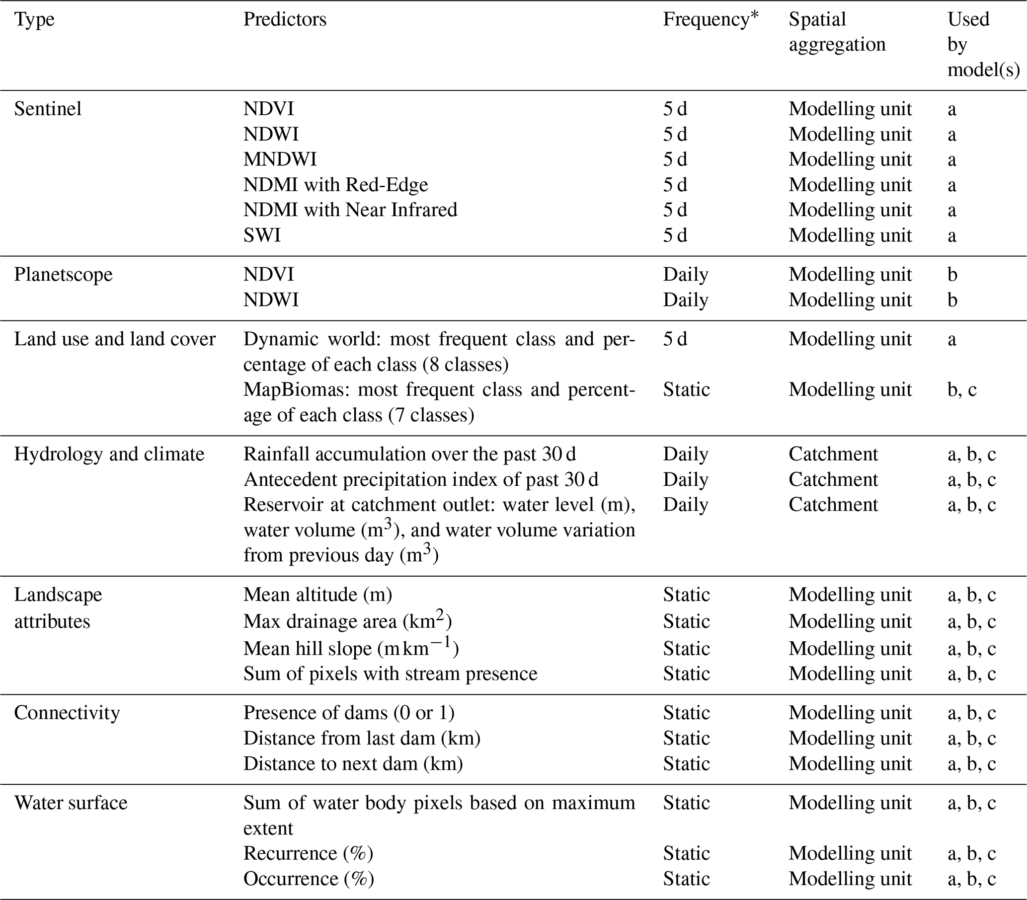
^* Satellite images frequency refers to availability under cloud-free conditions.

3.3 RivInt modelling framework

Initially, data are collected in the monitored river reaches and characterized in terms of water occurrence (see Sect. 3.2.3). Then these observations are used together with candidate predictors (Table 2) from various sources in the training of Random Forest classification models. This kind of models take into account decision trees derived from resampling the calibration dataset (Breiman, 2001). Each tree leads to a decision based on that particular calibration set, but a majority vote is taken on the final observations considering all trees. This way, dependence on calibration sets is potentially reduced. In the present study we implement the Random Forest classification model using the R package “randomForest” (Liaw and Wiener, 2002).

The importance of predictors is assessed by the increase in mean square errors during training when a predictor is randomly permuted within the tree. The “rfe” function (recursive feature elimination tool) in the R package “caret” selects the most suitable predictors (Kuhn, 2008). Recursive Feature Elimination (RFE) is an algorithm that applies a backward selection process to find the optimal combination of features and thereby selects the most important predictors (Gregorutti et al., 2017).

Through the elimination of unimportant predictors, we test whether it is possible to use fewer predictors to model intermittency. For this purpose, models with different data sources are tested in three groups of candidate predictors: (a) Model using Sentinel predictors to capture temporal dynamics (spectral indices and LULC data); (b) Model using Planetscope indices as dynamic predictors; and (c) Model using hydrological data as the only source of temporal dynamics. The specific predictors employed in each model are summarized in 2.

3.4 Model performance assessment

3.4.1 Cross-validation

A cross-validation procedure is carried out with data partitioning into training and testing datasets. We create a training set by randomly selecting 75 % of the observations. The test set consists of the remaining 25 %. The evaluation criteria are calculated on both train and test dataset.

The models use different quantities of observation data. Since satellite images are needed for models (a) and (b), images in concomitant dates (more or less one week from flight date) are considered in the training process. In Fig. 4, there are three concomitant dates for the Sentinel images (model a), and four dates for Planetscope (model b). For the last model (c), satellite images are not needed, that is why all five UAV surveys dates can be utilized for model training.

3.4.2 Evaluation criteria

We calculate several validation criteria so as to compare model performance. For a general assessment of modelling performance, out-of-bag error estimates (OOB) from Random Forest models training are assessed. The error estimates from trained models are then compared to a benchmark classifier (BC) based on the prevalence of a dominant class from the overall dataset. BC was the chance of error for that class: 1 minus prevalence of most frequent class. This way, we simply estimate the smallest error if we consider only the class frequency. Overall accuracy and balanced accuracy are calculated on training and testing datasets according to the following equations (Beaufort et al., 2019).

$$\begin{array}{}\text{(1)}& {\displaystyle }\mathrm{Accuracy}={\displaystyle \frac{\mathrm{TP}+\mathrm{TN}}{\mathrm{TP}+\mathrm{TN}+\mathrm{FP}+\mathrm{FN}}}\text{(2)}& {\displaystyle }\mathrm{Sensitivity}={\displaystyle \frac{\mathrm{TP}}{\mathrm{TP}+\mathrm{FN}}}\text{(3)}& {\displaystyle }\mathrm{Specificity}={\displaystyle \frac{\mathrm{TN}}{\mathrm{TN}+\mathrm{FP}}}\text{(4)}& {\displaystyle }\mathrm{Balanced}\mathrm{accuracy}={\displaystyle \frac{\mathrm{Sensitivity}+\mathrm{Specificity}}{\mathrm{2}}}\end{array}$$

where TP, TN, FP, and FN are true positives, true negatives, false positives, and false negatives, respectively.

To evaluate performance per class, a one-vs.-rest strategy was adopted: each water occurrence class was treated as the positive class in turn, with all remaining classes grouped as negative. This approach allows for consistent metric calculation across imbalanced classes. A conceptual diagram is presented in Fig. 6.

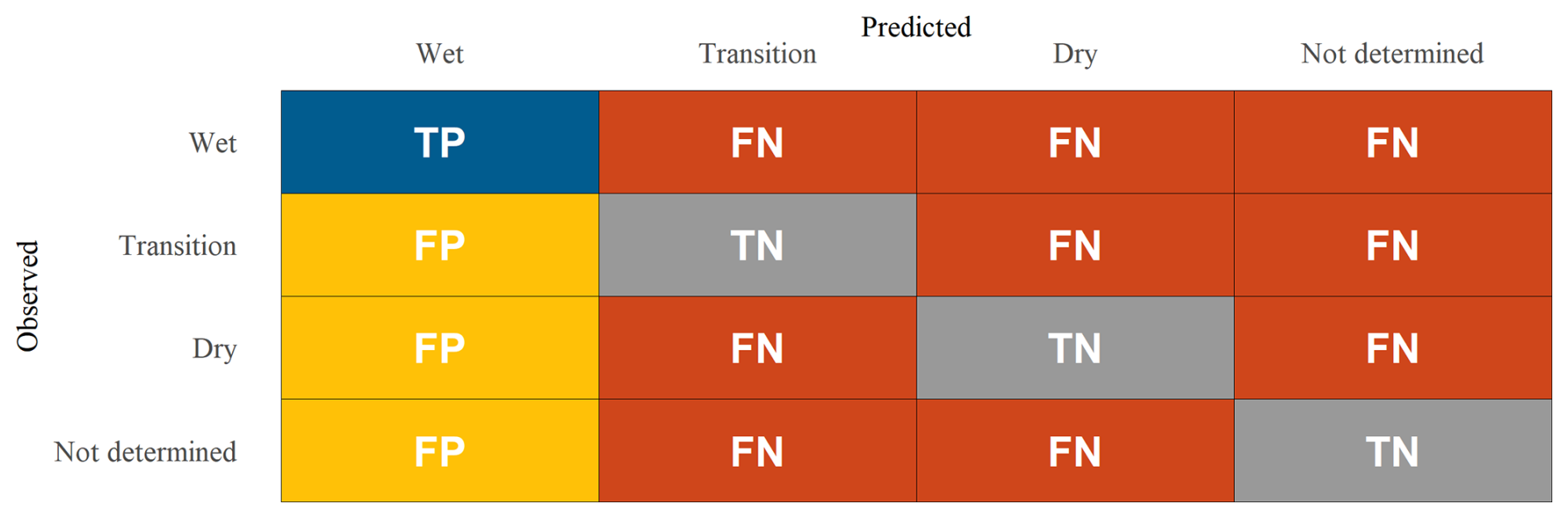
Figure 6 Confusion matrix used to compute classification performance metrics. Each color represents each of the possible combinations between predicted and observed classes: TP = true positives, TN = true negatives, FP = false positives, FN = false negatives. In this example, the “positive” class is “Wet”. This process was repeated for each class.

Overall accuracy (Eq. 1) reflects the proportion of correctly classified instances over the entire dataset and is useful for assessing general performance. However, it may be biased in datasets with imbalanced class distributions. To address this, we also report balanced accuracy (Eq. 4), which equally weights performance across classes by averaging sensitivity (true positive rate) and specificity (true negative rate). This metric provides a more reliable measure of performance when class sizes differ significantly. Together, these metrics allow us to evaluate how well each model discriminates among the different water occurrence classes, considering both general correctness and class-specific sensitivity.

3.4.3 Spatio-temporal extrapolation evaluation

In order to assess the extrapolation ability of the models, they are first trained and tested over river reaches during the period with available overlapping data (different for each model, see Fig. 4 and Sect. 3.4.1), then they are applied to the whole river on the remaining dates with the available 2022 data. For models (a) and (b), there are hardly any images outside the dry season. The third model (c) is applied during the whole year.

The results are evaluated in terms of temporal and spatial distribution: For temporal evaluation, the proportion of each class in the river is calculated at each date; And for spatial extrapolation, the number of days that each modelling unit has either a “Wet” or “Transition” class are analysed and assessed for plausibility. The number of observations with these classes is normalized and expressed as percentages.

4 Results and discussion

4.1 Observed water intermittency: UAV imagery

Figure 7 shows the spatio-temporal evolution of the four classes in the monitored reaches. As expected, the “Wet” class is more present in the most downstream reach and its share diminishes towards the dry season. This class represents the puddles and pools formed along the river. The “Wet” class mapping provides us with information on the distribution and connection of these puddles. Figure 7 illustrates that there are longer, more connected patches in the downstream reach and that they take longer to dry.

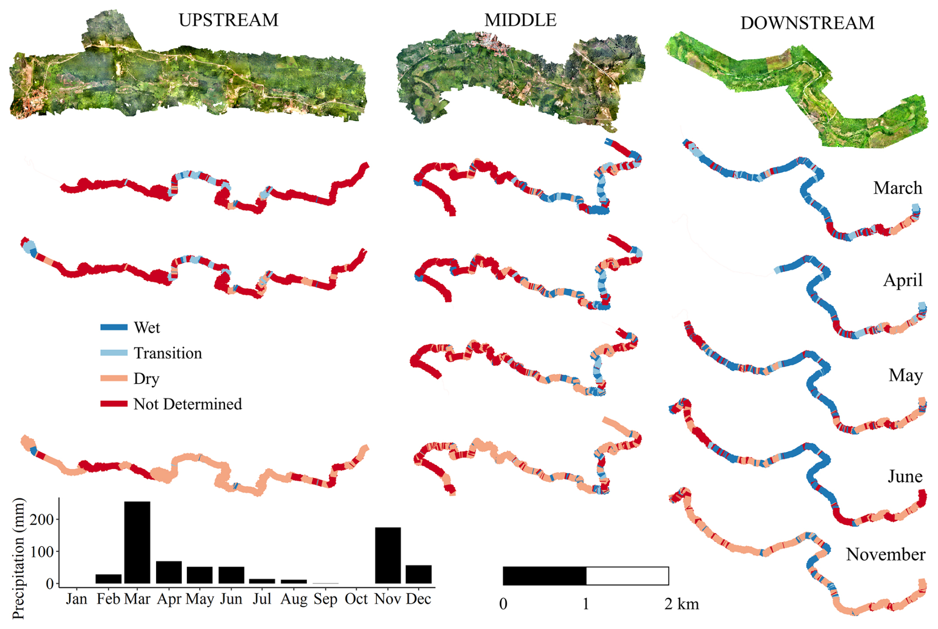
Figure 7 Occurrence of the four classes (Wet, Transition, Dry, and Not Determined) captured by UAV surveys of three reaches of the Umbuzeiro River (river flows from left to right). Each monitored section shows high-resolution classification of water occurrence in 1.0 m reaches. At the bottom left, see the monthly precipitation for the year 2022.

The “Transition” class is present especially in reaches with algae or herbaceous vegetation which make it difficult to distinguish between “Wet” and “Dry” patches. Macrophytes are known to impact surface water detection from remote sensing imagery, as in Zhang et al. (2018). In our classification, the impact is observed due to the presence of low vegetation in transition zones between “Wet” and “Dry”. We use this as a new class, so we can observe its patterns. Given its nature of occurrence, it is a very heterogeneous class.

“Transition” is more present in the upstream reach alongside the “Not Determined” class. Reaches are classified as “Not Determined” especially due to dense tree canopies which restrict visibility of the riverbed. Since most of the Caatinga vegetation is deciduous, this biome is nearly leafless during the dry season. The denser and full canopy is why the “Not Determined” class can be found more frequently during the rainy season and in narrower river stretches.

The “Dry” class is more present during the dry season, since the riverbed dries out almost completely and becomes visible due to leafless tree canopies. The decreased leaf area index during the dry season has already been explored in hydrological studies about this the study area (de Almeida et al., 2019; Vellame et al., 2024).

In general terms, we can say that “Wet” and “Dry” classes refer to open portions of the river, while “Transition” and “Not Determined” classes refer to areas with restricted visibility. The latter classes also represent narrower portions.

High-resolution UAV imagery enabled detailed visual classification of water occurrence classes. However, visual interpretation inherently brings uncertainty to the ground-truth generation. Ambiguous surfaces, such as distinguishing between “Wet” and “Transition” conditions, may introduce classification errors. To mitigate this uncertainty, ground-truth data was generated using the most frequent class within each modelling unit. This aggregation reduced spatial resolution of the analysis by summarizing 1 m classified segments into 100 m reaches. However, we also reduced the influence of local misclassification and increased robustness of the ground-truth representation. Field observations during the UAV campaigns also supported the interpretation of imagery and helped the classification.

4.2 Identification of important predictors

Overall accuracy in relation to the number of predictors is shown in Fig. 8a for each model. Through recursive feature elimination, we can observe that there is almost no gain in using all candidate predictors. The five most important predictors are sufficient to accurately predict river intermittency for all three models. Often times, the use of all candidate predictors adds more noise than important information to our predictions, selecting the most important predictors removes that noise and maintains enough information to classify the models (Gregorutti et al., 2017).

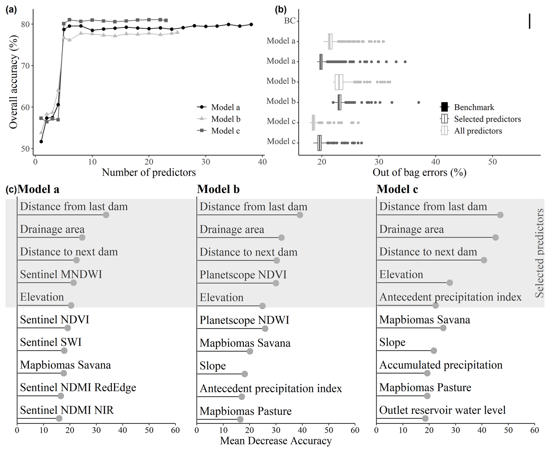
Figure 8 Random forest model evaluation and feature selection results for three predictor sets: (model a) Sentinel-2 indices, (model b) Planetscope indices, and (model c) hydrological variables. In (a) recursive feature elimination curves showing accuracy of the models as features are removed. In (b) out-of-bag (OOB) errors comparing models using all candidate predictors versus only the selected ones. BC denotes the benchmark classifier. In (c) mean decrease accuracy for the top 10 most important predictors in their respective model. Highlighted predictors were selected through recursive feature elimination based on their higher mean decrease accuracy.

The top 10 most important predictors for each model are shown in Fig. 8c. Model training determines their specific powers. Figure 8c displays the mean decrease accuracy (MDA) of each and highlights the selected predictors for each model. Variables with higher MDA values were selected because they have a greater impact on the predictive performance of the model. MDA reflects how much the accuracy of the model decreases when a given variable is excluded; thus, a higher MDA indicates that the variable provides important information for distinguishing between classes. By selecting variables with the highest MDA, we focused on those that most strongly influence the model’s ability to predict spatial patterns of intermittency. This approach helps identify predictors most relevant to distinguishing our water occurrence classes. Among the not selected predictors, the observed values for mean decrease accuracy is around 20 %. This corroborates with the maximum observed overall accuracy shown in Fig. 8a of around 80 % and means that in general 20 % of accuracy is lost when less important predictors are removed.

The same four predictors were selected for all three models: mean elevation, drainage area, distance from last dam, and distance to next dam. The difference for each model was the dynamic predictors. It was selected one spectral index for each of the remote sensing models: model (a) Sentinel MNDWI and (b) Planetscope NDVI. For model (c), antecedent precipitation index (30 d) was selected. The similarities among models show consistency on the relative importance of predictors.

Model performance patterns align with known physical drivers of river intermittency. For example, river reaches with small contributing areas were more frequently classified as dry. Conversely, regions with bigger contributing area tend to sustain surface water for longer periods (Costigan et al., 2017). This way, our models display the expected relationships between intermittency and landscape attributes (Fig. 8b); landscape attributes, such as mean altitude and maximum drainage area of the modelling units, are consistently selected as important predictors.

Catchment area or drainage area are sometimes identified as very important variables to classify streams as temporary or perennial (González-Ferreras and Barquín, 2017; Snelder et al., 2013). Altitude is another important variable to identify intermittent streams (D'Ambrosio et al., 2017; González-Ferreras and Barquín, 2017). Drainage area integrates upstream contributing catchment area and, by extension, potential water inputs to the channel network. Reaches with larger drainage areas are therefore more likely to sustain surface water for longer periods than headwater reaches with small contributing areas. This relationship is demonstrated in process-based studies of connectivity and its drivers in non-perennial rivers, which show that drainage area explains patterns and magnitude of flowing conditions (Zimmermann et al., 2014; Reynolds et al., 2015; Perez et al., 2020). This is also observed during periods of river network contraction, when headwater streams are pruned in dry years (Godsey and Kirchner, 2014; van Meerveld et al., 2019; Prancevic et al., 2025).

Altitude may further modulate river intermittency through its influence on catchment morphology and hydrological processes. Because our study focuses on a single river, altitude shows a consistent downstream gradient and scales with drainage area, with lower elevations corresponding to larger contributing areas. This relationship may differ when comparing multiple river reaches at similar altitudes across the catchment, where contributing areas might vary. In our study, the observed patterns of water presence along the river network are consistent with the influence of both drainage area and altitude and likely reflect their role in controlling flow permanence.

We note that the “distance from the last dam” is the most important predictor in all models. The reason for this may be the fact that even if there is a dam further ahead (“distance to the next dam”), a reach may be dry or wet due to other factors. Immediately after dams, however, reaches have a higher probability of being dry even in more favourable conditions (e.g. lower portion of catchment and during the rainy season).

This consistent selection of “distance to the next dam” and “distance from the last dam” as top predictors highlights the strong influence of anthropogenic flow regulation on surface water distribution. While the relevance of dams in altering flow regimes is widely acknowledged, our findings provide a fine-scale perspective on how even small impoundments can generate abrupt shifts in flow permanence along the network (Búrquez et al., 2024). Fencl et al. (2015) also showed that small dams individually and cumulatively alter lotic ecosystems. This is particularly relevant in semi-arid regions, where it is common to use small-scale storage and retention of surface water. However, as river networks become more intermittent due to climate-driven changes, this can be a reality in all climates (Messager et al., 2021).

Although predictors related to landscape attributes are well-established in hydrology, they gain new value here through their interaction with other spatial variables at finer resolution. For example, areas with high accumulation but located downstream of dams often remain dry, suggesting that topography alone does not explain surface wetness in human-modified catchments.

Dynamic predictors play an important role in observing temporal variation within a hydrological year. The spectral indices for each of the remote sensing models were previously employed to detect water. Sentinel MNDWI was used to study open-surface water in large water bodies and perennial rivers (Jiang et al., 2021; Li et al., 2020). Planetscope NDVI helped to successfully access LULC change detection and water class detection (Yao et al., 2024; Zhou et al., 2024). This shows that characteristics captured by these indices are important to classify reach intermittency.

We also acknowledge that other important attributes may have been omitted from our analysis. For example, we did not consider the role of groundwater in river intermittency, despite it being a well-established control on water presence along the riverbed (Conant et al., 2019). In many catchments, groundwater levels tend to converge toward the river channel in downstream reaches, contributing to spatial gradients in intermittency that may not be directly observable from surface-based remote sensing alone (Sophocleous, 2002; Snelder et al., 2013). In our study area, detailed investigations at a small scale (12 km²) have shown that runoff is mainly governed by precipitation, with negligible baseflow due to the short and highly concentrated events (De Figueiredo et al., 2016). In contrast, analysis conducted at a broader scale (20 000 km²) have shown different roles of groundwater on streamflow depending on the period of hydrological season (Costa et al., 2013). However, groundwater-level observations, hydrogeological information, and coupled surface–subsurface modelling outputs were not available for our study. Future work would therefore benefit from integrating such data to better disentangle the respective roles of climatic forcing, catchment properties, and groundwater storage in shaping non-perennial river behaviour.

Water accumulation in intermittent river seems to be governed by processes captured by landscape attributes (including human-made interferences) and satellite indices. The consistent selection of these predictors across models reinforces them as controls and indicators to water retention.

Our analysis considered the distance of dams as a proxy for potential human influence on water occurrence. However, detailed information on dam characteristics, such as reservoir capacity, was not available. These characteristics likely modulate the magnitude and spatial extent of dam impacts on downstream water presence and should therefore be considered in future studies.

4.3 Model performance evaluation

The out of bag errors (OOB) for all models are exhibited in Fig. 8b. We present OOB values for models (a), (b), and (c) trained with all candidate predictors and trained only with the selected variables shown in Fig. 8c. Among them, model (b) performs slightly worse, while models (a) with selected predictors and model (c) with all predictors achieved the best performances. These findings agree with Fig. 8a: both graphs make clear that the use of all predictors does not help to predict water occurrence classes in general. The benchmark classifier (BC) is based on a simple estimate of the dominant class from the overall dataset of observed classes. In our study, the “Not Determined” class is present in 43 % of observations, so the benchmark is 57 %. All trained models outperform the BC estimate.

Among the models, similar accuracy and balanced accuracy metrics are obtained (Table 3). Balanced accuracy accounts for class imbalance by averaging sensitivity (true positive rate) and specificity (true negative rate), providing a more reliable assessment when classes are unevenly distributed. Values are reported separately for training and testing datasets. In general, test scores are slightly higher than training scores, maybe due the smaller dataset. Since the partitioning of the observation dataset is random, it might also be due to our subset selection.

Table 3 Evaluation metrics for the three models considering train and test data. Model (a) with Sentinel predictors; (b) with Planetscope indices; and (c) with hydrological data.

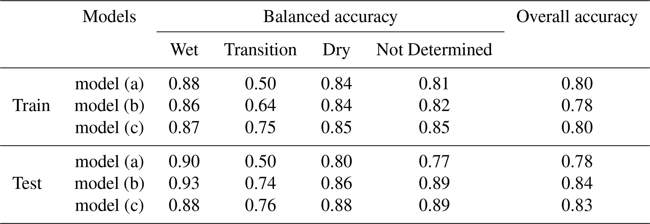
The classes have different balanced accuracy scores; yet for all models, “Transition” is the most difficult class to predict. This result is expected since this class has the smallest number of observations. The “Wet” class receives the highest balanced accuracy scores of all models, followed by the “Dry” class. The overall performance of “Wet” and “Dry” classes can be explained by their more homogeneous observations, whereas more heterogeneous observations can be expected from the “Transition” or “Not Determined” class. For “Not Determined” reaches, we take into account the lack of riverbed visibility, but this condition includes very heterogeneous vegetation types, for example.

An example of model performance can be observed in detail in Fig. 9. In it, we use one of the monitored reaches to demonstrate the comparison between observed and predicted classes for each modelling unit. Overall accuracy was 80 % for train and 78 % for the test data for this model (Table 3). Figures for other reaches and all models can be found in Appendix A.

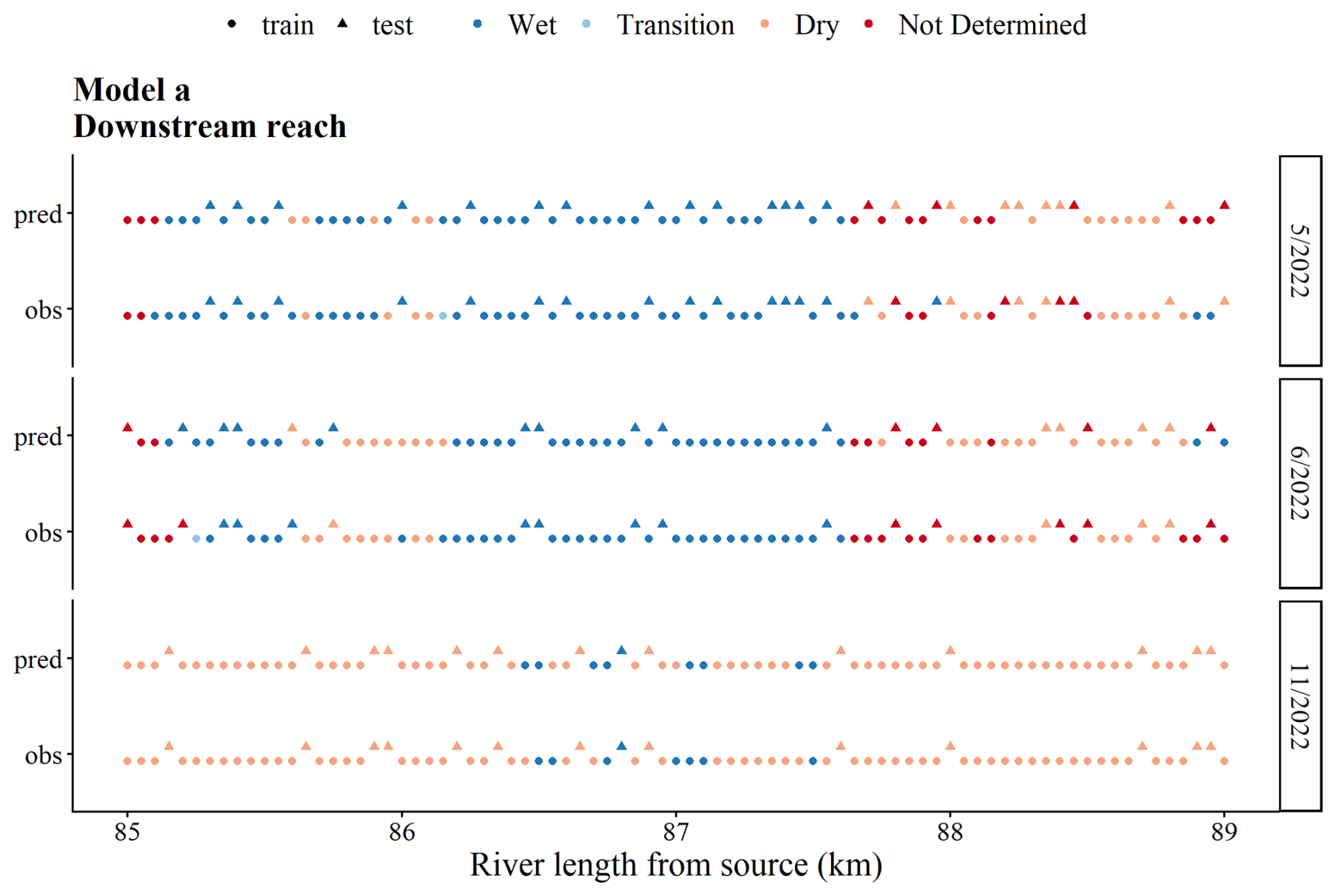
Figure 9 Modelling results comparing predicted (pred) and observation (obs) classes according to training and testing datasets. The example shows the results of model (a) in the downstream reach, for the months of May, June and November. Model (a) uses Sentinel predictors.

4.4 Umbuzeiro River: temporal extrapolation with models

The models are applied to the whole river with all available data, enabling the evaluation of model performance in spatial and temporal distribution. The proportion of each class in the whole river is shown in Fig. 10 for each model showing the temporal distribution for each class. Temporal variations along the year can also be observed in comparison to monthly precipitation. Model (c) is the least sensitive to temporal variation specially in the “Wet” class. The “Dry” and “Not Determined” classes vary along the year, but not in a consistent way. February and March, for example, are two of the months with the highest proportion of “Dry”, and they are normally part of the rainy season (De Figueiredo et al., 2016; Soares et al., 2024).

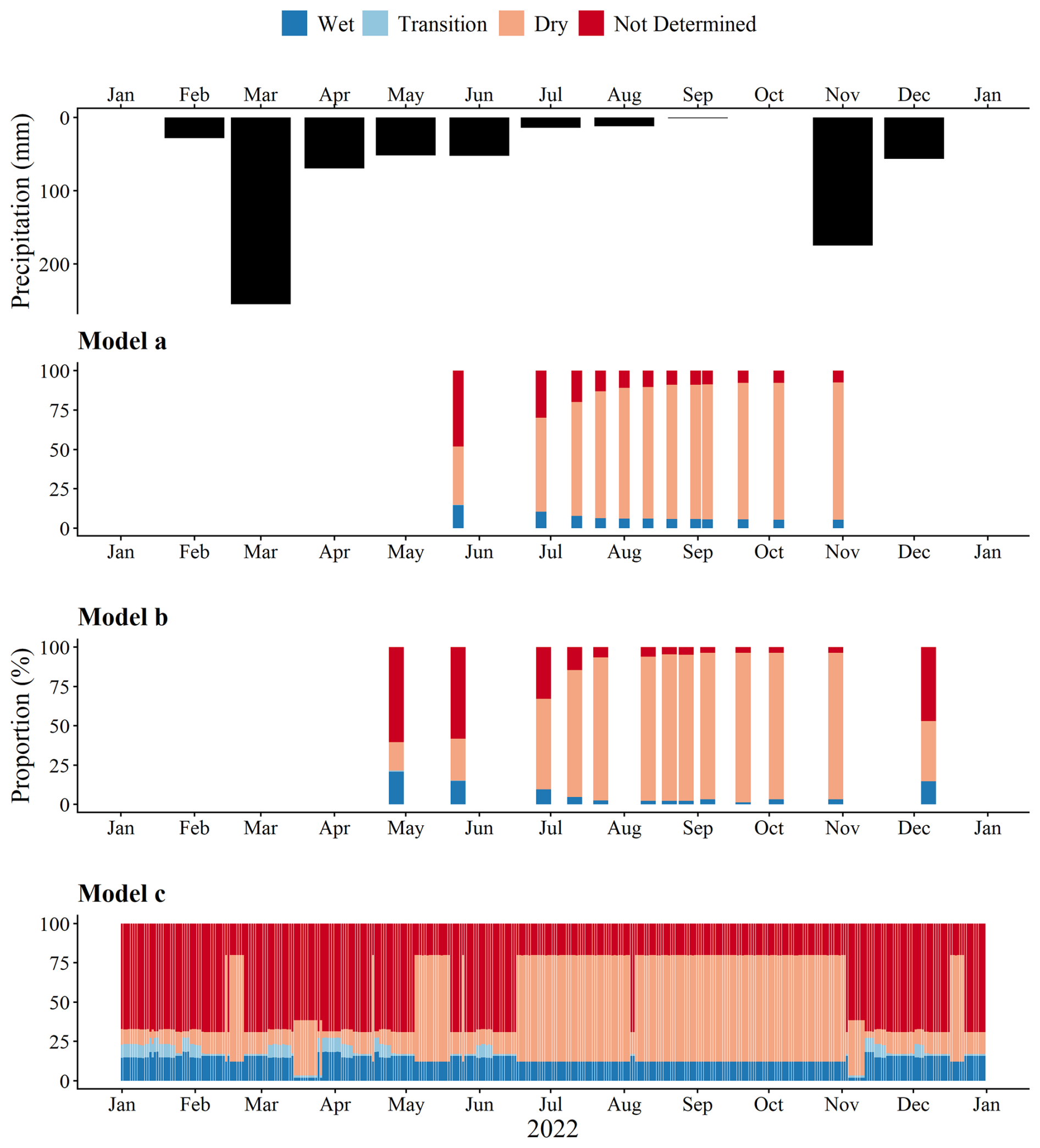
Figure 10 Proportion of each water occurrence class on the whole Umbuzeiro River. We apply the models with all available data for 2022 and show the results in comparison to monthly precipitation (top panel). Different number of simulations for each model depending on data availability (model a = 12; model b = 13; and model c = 365). Model (a) uses Sentinel predictors; (b) uses Planetscope indices; and (c) uses hydrological data.

In 2022, March is the rainiest month, still only a very small increase is observed for the “Wet” and “Transition” classes. The pattern of drying predicted by Model (c) may reflect lagged hydrological responses not captured by the antecedent precipitation index for that month. In contrast, the prediction for November coincided with isolated rainfall events that triggered surface water reappearance, which may be better captured by the antecedent rainfall.

Since Model (c) only uses rainfall data as dynamic predictor, it was expected to follow the seasonal behavior of water occurrence. However, the poor performance of this model in its application to the whole river indicates that it cannot extrapolate local-trained conditions considering only the landscape attributes together with precipitation.

For both models (a) and (b), there is a gradual decrease of “Wet” and “Not Determined” classes as the dry season progresses. While the “Wet” class gives information about the occurrence of puddles, the “Not Determined” class gives an idea of how dense the vegetation is. Since we are dealing with deciduous forest, a higher proportion of this class means that vegetation has leaves and is covering the riverbed. The “Dry” class proportion increases during the dry season.

The better plausibility of models (a) and (b) is due to more detailed and distributed information added to the models. This suggests that satellite-driven variables may better capture ecologically meaningful signals of intermittency, possibly due to their ability to represent spectral landscape responses. It is also possible to observe the complementary convergence of vegetation and water-related satellite indices and landscape attributes, which reinforce each other as physical controls (or responses) related to water retention.

Although the simplified model (c) performs satisfactorily in the test data, it does not provide a good temporal extrapolation of the river drying dynamic. This way, the dynamic predictor of model (c) (antecedent precipitation index for the last 30 d) is not sufficient to accompany the temporal river dynamics when training reaches are extrapolated. Other figures showing the spatial and temporal performance for all models can be found in Appendix B.

4.5 Umbuzeiro River: spatial performance of models

The models are applied to the whole river, and the number of days with either “Wet” or “Transition” classes are calculated for each spatial unit: they indicate that there is “water in the riverbed” (WIR). In Fig. 11, it is possible to see the spots with more WIR-observations. Due to data availability, the highest possible numbers display different variations depending on the model: for models (a) and (b), it ranges from 0 to 12 or 13 observations, and for model (c) it differs from 0 to 365 observations with either of the two classes. Because of this, the number of observations is normalized and expressed as percentages. It is possible to observe that similar spots in all three models are prone to wetter conditions.

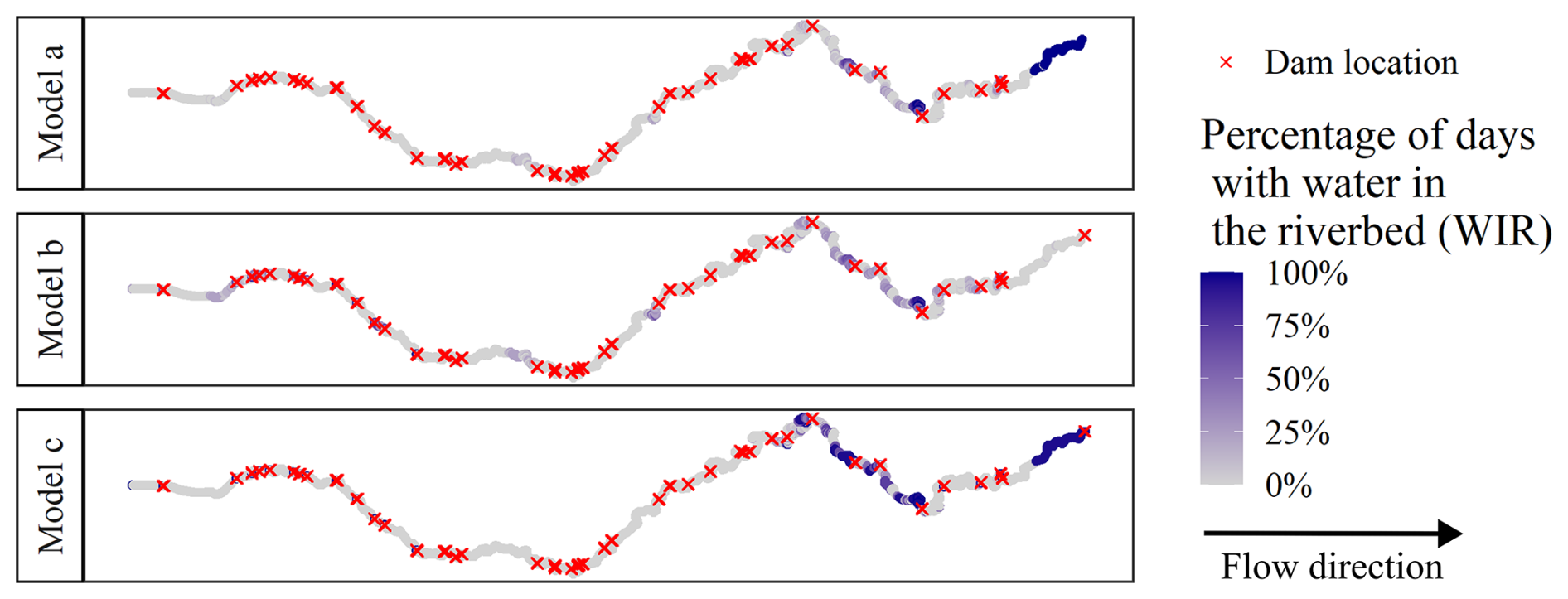
Figure 11 Observations with water in the riverbed (WIR), that is when the reach presents either “Wet” or “Transition” classes. The number of observations is normalized and expressed as percentages. Model (a) uses Sentinel predictors; (b) uses Planetscope indices; and (c) uses hydrological data. Red crosses indicate dam locations.

Regarding the spatial distribution of areas with higher WIR, the graphic shows to its extreme right that only models (a) and (c) identify the Benguê reservoir as a place with frequent “Wet” or “Transition” classes, for example. This is important because the reservoir is not part of the model training, but still a key factor to assess streamflow in the catchment. This way, models (a) and (c) outperform model (b), when they identify important reservoirs as areas prone to pounding. Model (a) is even more specific in this respect, and indicates mainly areas in the lowest part of the basin. The identification of areas prone to wetter conditions is very important even in the smallest of scales because they can be key areas for river ecology, for instance Fencl et al. (2015).

Analyzing our findings, we see that model (a) seems more plausible than the others, as it is able to extrapolate and produces smaller OOB errors. During training, model (b) performs worse than the others and generates greater OOB errors. It is also less conceivable than the others regarding spatial distribution of areas prone to wetter conditions. Model (c) presents small OOB errors and good accuracy for training and test datasets. However, the temporal analyses of its extrapolation to the whole river shows that this model can not predict river dynamics. Model (a), on the other hand, extrapolates well as was proved by both our temporal and spatial analysis.

Considering that model (a) modelled the drying and rewetting dynamics of the riverbed and spotted areas prone to water occurrence, it is shown as suitable for application on narrow rivers to observe classes of water occurrence. This way, we can model how intermittent is the river or how it changes from one year to another. The mapping of intermittency of water occurrence throughout the river in non-perennial rivers is important to analyse the migration and resilience of species, to understand their habitat and to conduct studies on intermittent river dynamics (Sarremejane et al., 2017).

4.6 Work limitations

Evaluating our work, we begin by pointing out that we opt for a better observation quality versus quantity. Instead of mapping the entire riverbed (high quantity of observed areas) with UAV flights, for example, we decide to map and observe certain reaches in detail multiple times (better quality). This way, we add a higher time resolution and favour the ability to model temporal dynamics, instead of observing more areas. In addition, most of the extension of the river flows through private properties, so access is limited. Yet access is important because we need to be at an acceptable distance from the UAV platform during the flight. Take-off and landing should also be closer to the actual flight area. This way, we save battery and get better area coverage per flight.

In order to provide a general assessment of classification, the processing of each UAV image includes orthomosaic generation for the visual distribution of river reaches into intermittency classes. Through this orthomosaic generation we acquire one scene per monitored reach. Each reach is on average 5 km long and divided in 1.0 m reaches for classification. In total, 12 flights are performed and so we obtain a total of 60 000 reaches to be visually categorized for observation classes.

Although high-resolution UAV imagery enabled detailed visual classification of flow permanence classes, the method relied on expert interpretation without direct hydrological measurements such as streamflow or water level data. This introduces potential subjectivity, particularly in distinguishing between “Wet” and “Transition” conditions. Field observations were conducted during the UAV campaigns and helped inform classification, but were limited to qualitative assessments of ponded water, as no surface flow was observed during the study year.

We based our analysis on data from a single hydrological year. While this approach allowed for the capture of short-term hydroclimatic variability, it limits the model’s capacity to generalize across years with different rainfall patterns. Future studies including multi-year data and alternative temporal windows could help address this limitation.

Additionally, we acknowledge the potential value of integrating other dynamic hydrological variables, such as soil moisture and evapotranspiration, into predictive models of flow intermittency. These variables are relevant for ecohydrological modeling, particularly in dryland environments. However, in the context of this study, such data were unavailable at the spatial and temporal resolutions required to support fine-scale modeling.

The use of either wing-based or copter platforms have different advantages and disadvantages: while wing-based UAV has an average coverage of 150 ha per flight, the copter UAV mean coverage is only 20 ha per flight. For example, we cover the whole downstream reach with only two flights of the wing-based platform, whereas we need six flights for coverage of the same river reach with the copter platform. This is why we try to exclude unnecessary areas and turns as much as possible and capture only the riverbed area. We do our best to keep flight altitude stable between platforms at around 100 m. It could be increased in order to have faster coverage, but this decreases final ground resolution. Our wing-based platform also has multispectral cameras that would be useful for spectral indices based on UAV data; however, the lack of light uniformity during flights makes uniform reflectance correction and the use of spectral indices not possible.

Moreover, we use the spatial definition of the modelling units for both the response variable and most landscape-based predictors. Arguably, water occurrence in a river reach may be affected by landscape property beyond the 100 m radius. Furthermore, we do not take into consideration if non-overlapping units performed the same way or if the circular shape of the areas influences the outcome.

The results of our modelling approach is given as one class per modelling unit, i.e. categorical response variable. Instead, predicting the fraction of each class within the modelling unit would yield a more differentiated picture. What is more, implementing some proxies for spatial auto-correlation (e.g. intermittency state of neighbouring units) could potentially improve the spatial coherence of the predicted patterns.

As for our choice of predictors, we recognize that spatial resolution and ease of access vary greatly among them. The selected predictors are consistent among models; but great importance is given to dam identification. Both “distance from” and “distance to” dams ranked as highly important in model performance, and they already represent half the number of static predictors. In our study area, we identify many different types of damming structures – ranging from small rural weirs to larger reservoirs – future studies could benefit from classifying them into distinct functional or structural categories.

The manual mapping of small dams enabled a more realistic representation of water retention in the basin. However, dam mapping may also limit applicability of our model to other regions as it requires considerable manual effort and, potentially, familiarity with the study area. That said, the methodology is adaptable: similar analyses can be replicated using global datasets such as the Global Surface Water Explorer (Pekel et al., 2016), which provides historical water occurrence based on Landsat imagery.

Finally, although Sentinel-2 data used in model (a) yielded strong results in our study area, the performance of its spectral indices – particularly MNDWI – may decline in more heavily forested or topographically complex catchments. In these cases, alternative data sources or higher resolution sensors may be needed to accurately identify surface water. However, it may be that dense vegetation can also serve as an indirect indicator of groundwater presence or surface wetness, and these segments were conservatively labeled as “Not Determined” in our classification.

5 Conclusions

The present study aims to map and model the spatial and temporal dynamics of intermittency. We use field measurements to characterize intermittency in monitored reaches, and Random Forest models to extrapolate the information along the Umbuzeiro River. During field data acquisition, we map water occurrence in four intermittency classes: “Wet”, “Transition”, “Dry”, or “Not Determined”. It is important to observe spatial and temporal variation in the monitored reaches; these data are the basis to water occurrence modelling.

The “Wet” and “Dry” classes follow the rainy season dynamics, and the longer wet patches are present in the most downstream section. The “Transition” class is very heterogeneous because it represents areas with mixed information: such as wet/dry patches with algae and sparse vegetation. During the rainy season, the vegetation has full and dense canopies, that is why the “Not Determined” class, i.e. the river reaches where we cannot see the riverbed from the UAV-imagery, can be found more frequently during the rainy season and in narrower river stretches. This feature represents a major source of uncertainty, limiting the available data acquired through optical remote sensing.

For modelling, first we gather candidate predictors and select the most important ones. This way, we identify the main drivers of intermittency in our study area. Then we train different models depending on the source and type of dynamic variable used. We select consistent static predictors in three models, and dynamic predictors that differ in each model. The static predictors are: mean altitude, drainage area, distance from last dam, and distance to next dam. The dynamic predictors are: for model (a) Sentinel MNDWI; (b) Planetscope NDVI; and (c) Antecedent precipitation index (30 d). We find that the use of a higher number of predictors compromises model efficiency. All model variants successfully model intermittency of monitored river reaches with an accuracy of around 80 % for both test and training.

Model extrapolation to the whole river enables us to evaluate model performance in spatial and temporal distribution. Models (a) and (b) capture the temporal dynamics in model extrapolation to the whole river. Model (c) shows little ability to model the drying of the river as the dry season advances. Regarding the spatial distribution of water occurrence, model (b) performs worse for not being able to map important spots of water accumulation. Models (a) and (c) captured similar areas that are prone to wetter conditions. Therefore, we conclude that model (a), based on Sentinel data, is the best choice with a good temporal and spatial response thanks to its ability to extrapolate. One reason for this, is that the use of Sentinel MNDWI in model (a) aggregates enough spatial information (that changes from one image to another) so the model can better simulate water occurrence classes. The findings presented here emphasize the possibility to use this index even in narrow non-perennial rivers.

The modelling framework developed in this study contributes to a broader understanding of flow intermittency as a spatially complex and highly dynamic process over time. The integration of high-resolution predictors, especially related to dam presence, landscape attributes and satellite indices, offers a scalable and adaptable approach for mapping wetness conditions in other dryland river systems. These insights are particularly relevant in the context of increasing climate variability and water stress, as they point to key landscape features that can be targeted for monitoring or management. Our results demonstrate that even in the absence of extensive hydrometric data, meaningful patterns can be derived from the careful integration of remote and field-based observations.

However, the lack of explicit consideration of groundwater–surface water connectivity is a limitation of our study. Groundwater may have a strong control on river intermittency, particularly during recession periods following flow events. Although the remote-sensing-based framework successfully captures spatial patterns of intermittency, incorporating groundwater observations or hydrogeological information would improve process understanding and help refine predictions of flow persistence in non-perennial rivers. Addressing this limitation represents an important direction for future research.

The application of the results presented here is relevant to both ecological and hydrological studies so as to understand and evaluate river dynamics and pool formation. For hydrological studies, dry and wet patterns can be used to better understand streamflow formation, drying and wetting frequency, and the impact of damming structures on connectivity. From an ecological perspective, mapping the temporal dynamics of wet and dry conditions at the river scale is crucial for assessing species migration and resilience, characterizing habitat availability, and analysing key components of river metabolism, such as gross primary production and ecosystem respiration.

Appendix A: Model performance in monitored reaches

Model performance can be observed in detail in the following figures (Figs. A1, A2 and A3). Each figure represents the performance of one model in all the monitored reaches. We see in the figures the different number of observations for the respective models and reaches.

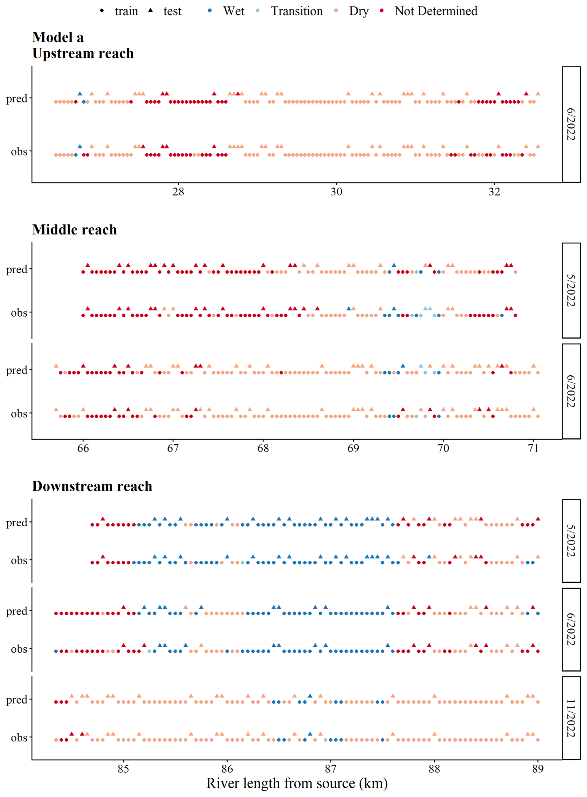
Figure A1 Modelling results comparing predicted (pred) and observation (obs) classes considering training and testing datasets. Example shows the results in all reaches of model (a) for the months May, June and November.

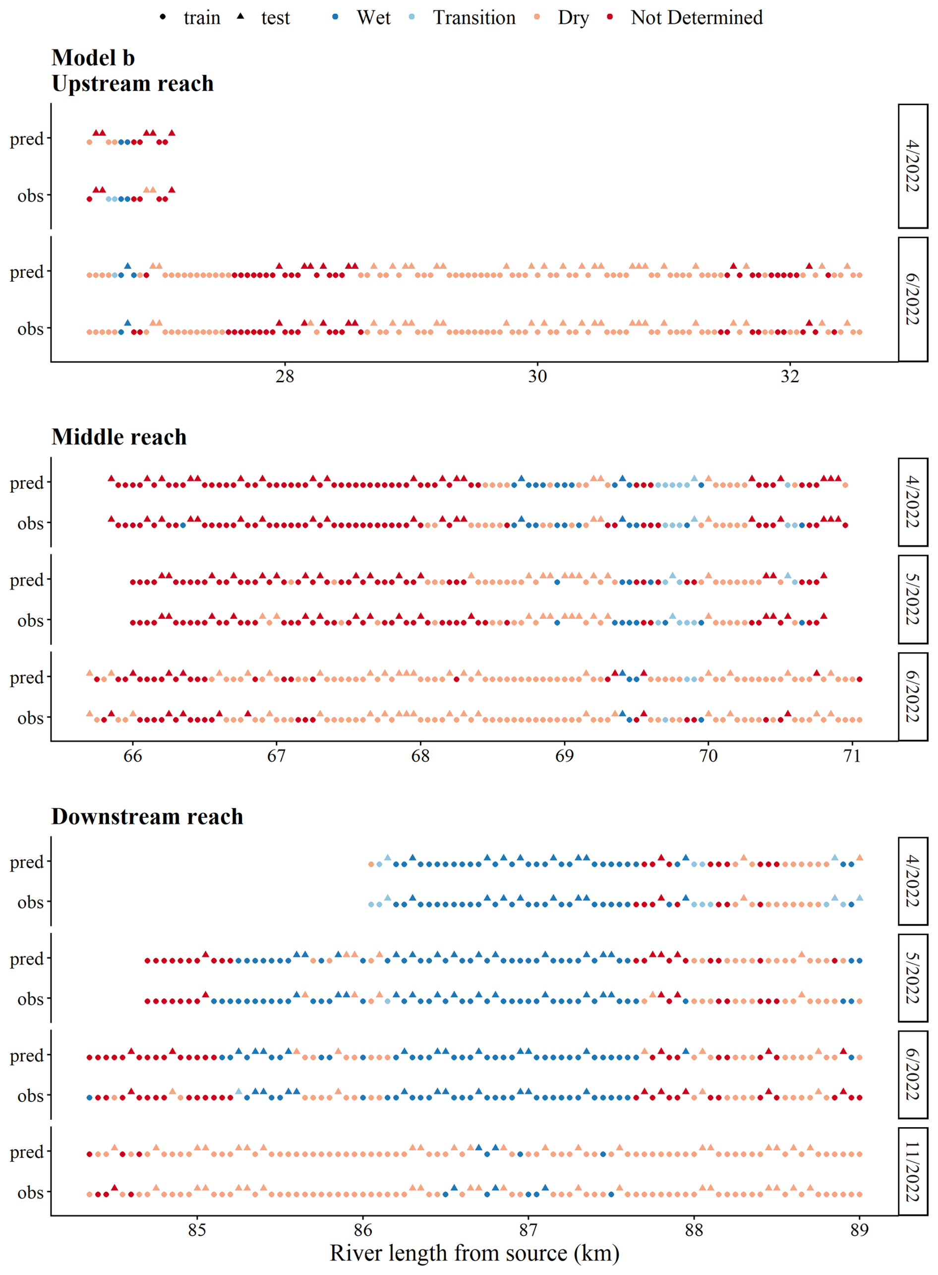
Figure A2 Modelling results comparing predicted (pred) and observation (obs) classes considering training and testing datasets. Example shows the results in all reaches of model (b) for the months April, May, June and November.

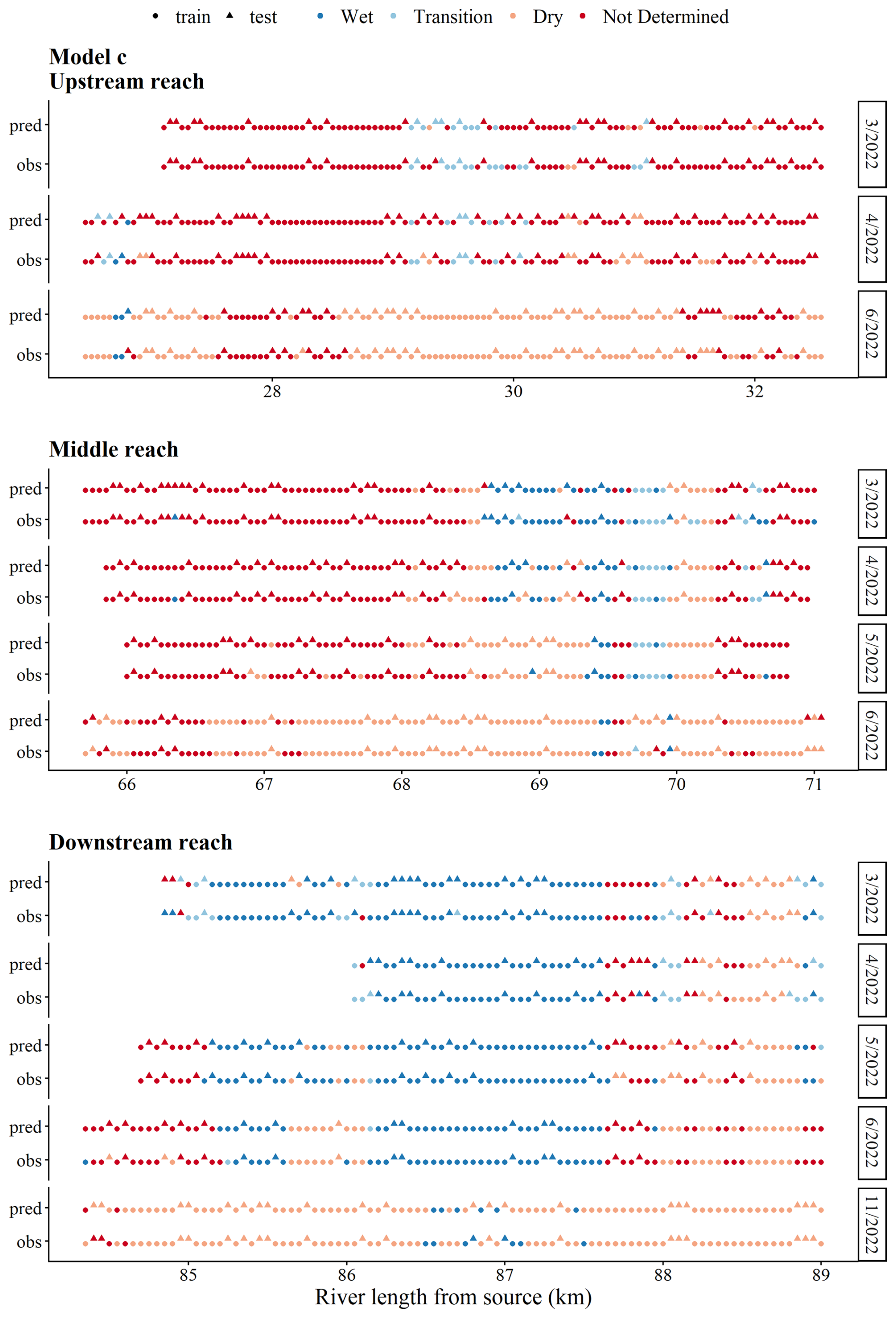
Figure A3 Modelling results comparing predicted (pred) and observation (obs) classes considering training and testing datasets. Example shows the results in all reaches of model (c) for the months March, April, May, June and November.

Appendix B: Model application to the whole river

Model application can be observed in the following figures (Figs. B1, B2 and B3). The model is applied to the whole river in all available dates. Each figure represents one model in all dates. We see in the figures the different numbers of available dates for the respective models.

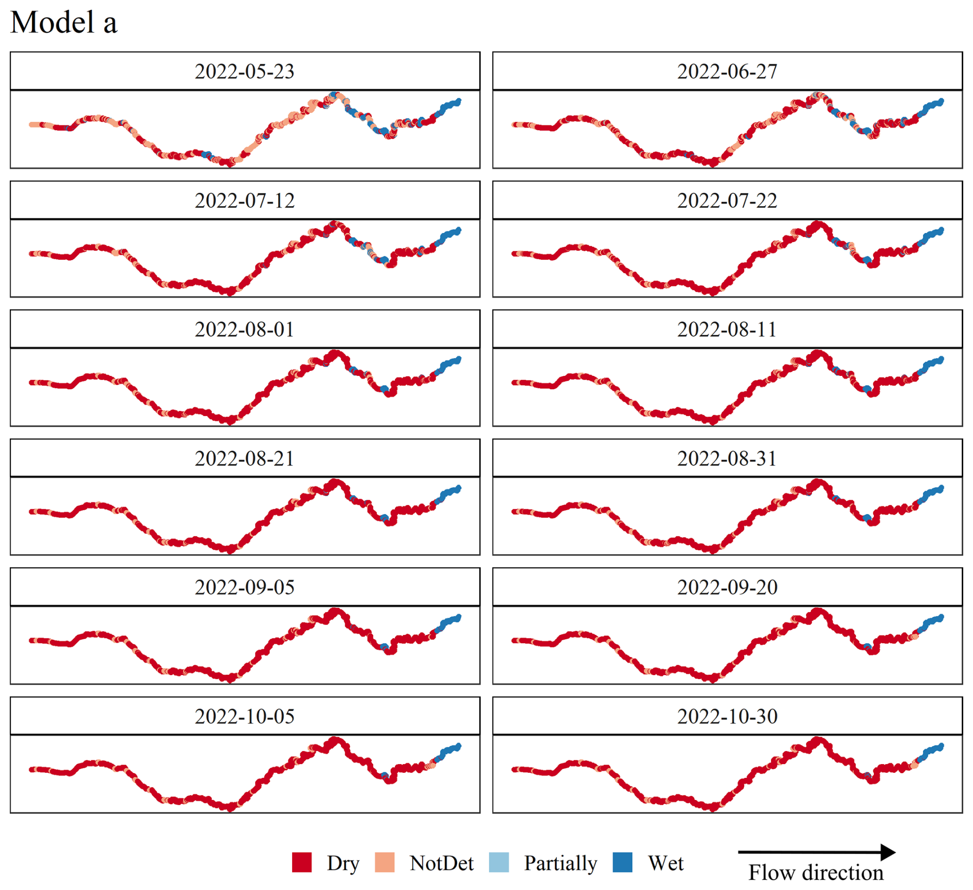
Figure B1 Spatial distribution of predicted riverbed conditions for selected dates in 2022 based on model (a). Each panel corresponds to a specific observation date, with colors representing the predicted water occurrence class for each unit along the river.

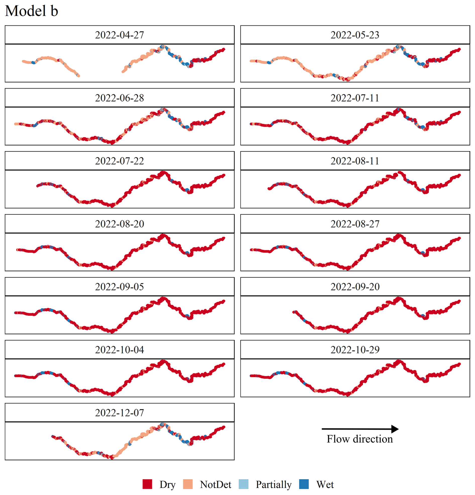
Figure B2 Spatial distribution of predicted riverbed conditions for selected dates in 2022 based on model (b). Each panel corresponds to a specific observation date, with colors representing the predicted water occurrence class for each unit along the river.

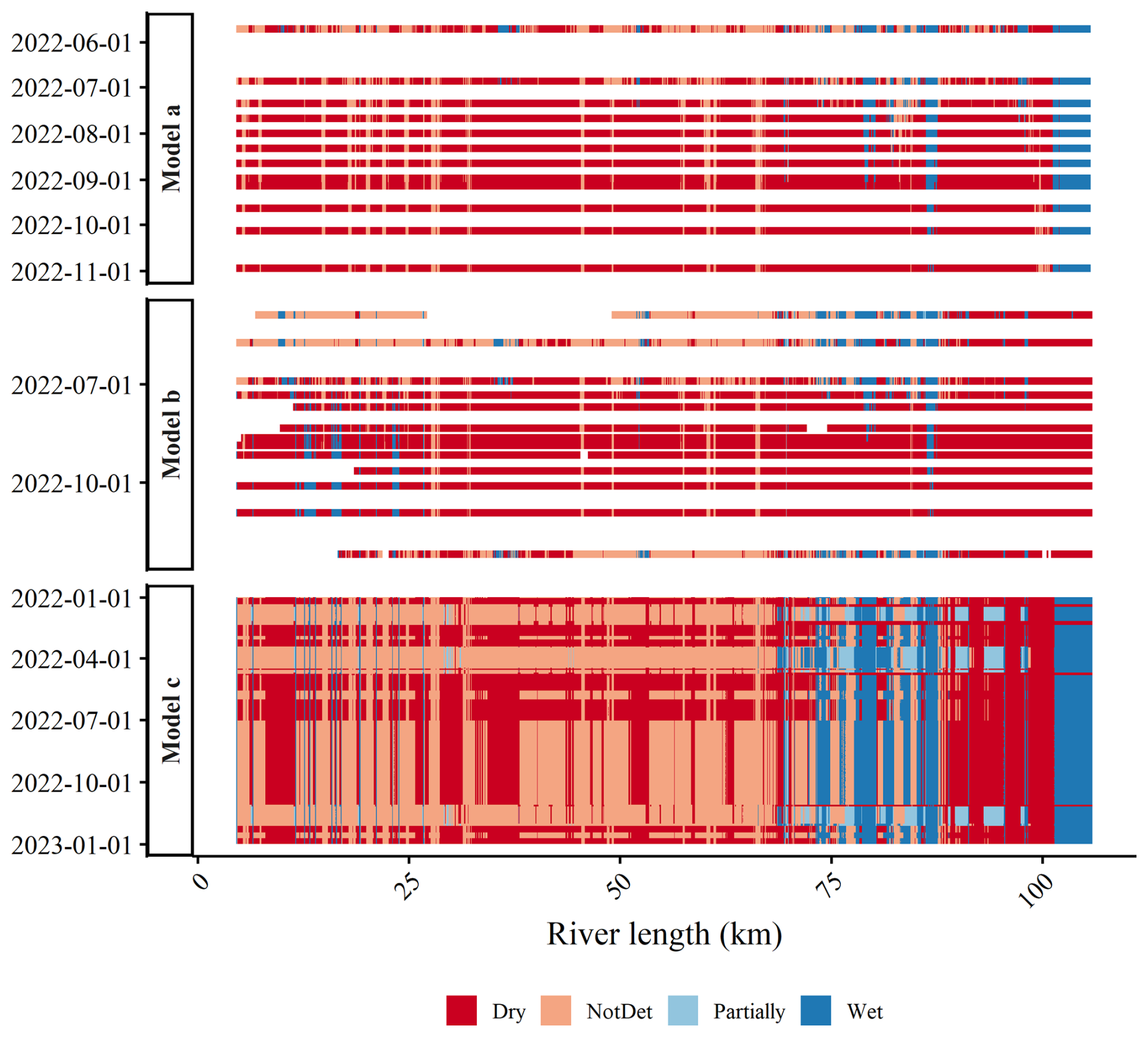
Figure B3 Spatiotemporal diagram of predicted riverbed conditions for 2022. Here we show the application of all three models in the whole river. The x-axis represents the river distance (from upstream to downstream), and the y-axis represents time (January–December 2022). Colors indicate the predicted water occurrence class for each unit along the river.