
the Creative Commons Attribution 4.0 License.
the Creative Commons Attribution 4.0 License.
 | 18 Nov 2026
Process diagnostics of snowmelt runoff in global hydrological and land surface models – Part 2: Are more complex models better?
Xiangyong Lei
Haomei Lin
Kaihao Zheng

The added value of increased process complexity has long been a central yet unresolved question in hydrological modeling, particularly for snowmelt runoff (SMR), where multiple physical processes interact in complex ways. In this study, we develop a Tree-Based Model Complexity Scoring (TBMCS) method to quantify the complexity of snow-related processes across 13 global hydrological and land surface models. We then systematically revisit the important linkage between model complexity and model performance in three distinct SMR characteristics, i.e., total runoff (Qsum), peak flow (Qmax), and centroid timing (CTQ) of runoff in the snowmelt period. Further, we assess how the basin complexity (as delineated by 1455 snow-dominated basins), forcing difference and calibration status can modulate this linkage. Results show that (1) models differ substantially in their physical process representations, with the largest divergence in melting process treatments, followed by sublimation, interception and rainfall-snowfall partitioning processes. (2) Model performance for Qsum and Qmax shows only weak associations with model complexity. Interestingly, we find a positive correlation between snow-process complexity and model performance for CTQ (r=0.32). This relationship remains positive under high basin complexity (r=0.35) and becomes statistically significant within the subgroup of models driven by GSWP3–W5E5 (r=0.81, P<0.05). These findings suggest that greater snow-process complexity may be associated with improved simulation of runoff timing. Finally, we also find that (3) model performance depends more on systematic and balanced representations of key processes than on model complexity alone. These findings suggest that greater snow-process complexity may be associated with improved simulation of runoff timing but not runoff magnitude. By providing a quantitative and process-traceable framework for assessing model complexity, this study helps identify which process representations are most relevant for improving SMR simulations under complex environmental conditions.
- Article
(12617 KB) - Full-text XML
- BibTeX
- EndNote


Hydrological models play a central role in global water resources management, flood forecasting, ecosystem protection, and climate-impact assessment. With advances in computational capacity and improved understanding of hydrological and land-surface processes, these models have evolved from early conceptual frameworks to increasingly complex and process-based systems. Added complexity can improve physical realism by representing more processes and interactions, but it does not necessarily guarantee better model performance. A long-standing body of literature has shown that greater complexity may introduce additional parameters, calibration difficulty, equifinality, structural uncertainty, and computational burden (Beven, 1993, 2006; Savenije, 2001; Schoups et al., 2008; Arkesteijn and Pande, 2013; Merz et al., 2022). At the same time, simplified or idealized models remain valuable because they can isolate key mechanisms and retain essential system behavior without unnecessary structural detail (Reed et al., 2025). Therefore, the key question is not simply whether more complex models are better, but rather under what conditions, for which processes, and for which performance metrics added complexity becomes beneficial.
This question is particularly relevant in snow-dominated basins. Compared with rainfall-driven runoff, snowmelt runoff (SMR) involves a cascade of coupled processes, including rainfall–snowfall partitioning, canopy interception, sublimation, snow accumulation, melt-energy exchange, liquid water transfer, and snow–albedo feedbacks (Lei et al., 2025). These processes jointly determine not only the amount of meltwater available for runoff, but also the rate and timing of meltwater release. The coexistence of these interacting processes creates a high degree of physical complexity, making SMR an appropriate testbed for examining how process representation influences model behavior. However, the potential value of added complexity is unlikely to be uniform across all SMR characteristics: runoff volume, peak flow, and runoff timing may respond differently to changes in model structure, parameterization, and calibration.
Existing hydrological and land surface models differ substantially in how snowmelt-related processes are represented. Depending on their primary objectives and historical development, some models adopt simplified formulations or rely partly on calibration to compensate for omitted processes, whereas others explicitly represent additional energy- and mass-exchange mechanisms. For example, some models use empirical degree-day formulations for snowmelt, while others resolve snowmelt through more physically based energy-balance schemes involving radiative transfer, albedo evolution, or snow-aging effects. Similar differences also exist in the treatment of sublimation, interception, and rainfall–snowfall partitioning. These structural differences make it difficult to compare models and to understand how process complexity affects performance. Moreover, model complexity itself is challenging to quantify consistently (Best et al., 2015; Orth et al., 2015; Merz et al., 2022). Previous efforts have often relied on qualitative descriptions, schematic illustrations, or broad structural classifications (Telteu et al., 2021; Müller Schmied et al., 2025), which are informative but do not provide a unified quantitative basis for evaluating process-level complexity across models.
The broader hydrological literature also suggests that the complexity–performance relationship is strongly context dependent. Multi-model studies have shown that different model structures can perform differently under contrasting climate conditions, and that no single level of complexity is universally optimal (Seiller et al., 2012; Horton et al., 2022). In climate-impact and data-scarce applications, model complexity can interact with forcing uncertainty and calibration strategy, making it difficult to attribute performance differences to structure alone (Ludwig et al., 2009; Knoche et al., 2014; Muñoz et al., 2021). For snow-related modeling, previous studies have similarly found that moderately complex models can outperform both overly simple and overly complex alternatives (Valéry et al., 2014), and that intermediate-complexity models may provide the best regional-scale performance (Merz et al., 2022). These findings highlight the need to move beyond a binary framing of “more complex versus simpler” and toward a more diagnostic assessment of when added process representation is useful.
Despite this progress, several limitations remain. First, model complexity is often characterized using parameter counts or broad structural categories, which may not reflect the mechanistic representation of individual snow-related processes. Second, many previous studies are based on limited model ensembles or basin samples, which restricts the generalizability of their findings under large-scale and environmentally heterogeneous conditions. Third, performance assessments often emphasize aggregate runoff metrics and give less attention to snowmelt-specific characteristics such as total runoff (Qsum), peak flow (Qmax), and centroid timing (CTQ). These three characteristics are directly relevant to water resource utilization, flood hazard prevention, and water resource management, respectively, but they may respond differently to model structure and process representation. As a result, it remains unclear whether added snow-process complexity improves SMR simulation in general, or only for particular runoff characteristics and basin conditions.
To address these gaps, this study proposes a unified and quantitative framework to characterize model complexity in SMR processes. We compile 13 state-of-the-art large scale hydrological, land surface, and dynamic vegetation models that span a broad spectrum of complexity. These include six ISIMIP2a water sector models (PCR-GLOBWB (Sutanudjaja et al., 2018), DBH (Tang et al., 2006), VIC (Liang et al., 1994), MATSIRO (Pokhrel et al., 2014), CLM40 (Oleson et al., 2010), LPJML (Schaphoff et al., 2018)) and seven ISIMIP3a models (CWATM (Burek et al., 2020), H08 (Hanasaki et al., 2008), HYDROPY (Stacke and Hagemann, 2021), JULES-W2 (Best et al., 2011), MIROC-INTEG-LAND (Yokohata et al., 2020), ORCHIDEE-MICT (Guimberteau et al., 2018), WATERGAP2-2E (Müller Schmied et al., 2024)). The ensemble is not intended to be an exhaustive set of all available models (Hou et al., 2023; Guo et al., 2024), but it aims to provide a representative and sufficiently diverse testbed for evaluating the complexity–performance relationship.
Building on the evaluation framework established in Part 1, this study focuses on explaining, rather than further diagnosing, differences in SMR simulation across models. Specifically, we aim to (1) develop a Tree-Based Model Complexity Scoring (TBMCS) method to quantify process complexity in snow accumulation and melt; (2) apply this framework to a large ensemble of 13 state-of-the-art models across 1455 snowmelt-domain catchments worldwide; and (3) examine how model complexity relates to model performance and robustness for key SMR indicators, namely Qsum, Qmax, and CTQ. Thus, while Part 1 addresses how models perform (Lei et al., 2026), Part 2 explores how differences in snow-process complexity relate to these performance patterns and what this means for future model development.
2.1 Models and study regions
This study uses 13 models from ISIMIP2a/3a as the testbed for examining the relationship between model complexity and model performance, including six global hydrological models (GHMs: PCR-GLOBWB, VIC, CWATM, H08, HYDROPY, and WATERGAP2-2E), six land surface models (LSMs: DBH, MATSIRO, CLM40, JULES-W2, MIROC-INTEG-LAND, and ORCHIDEE-MICT), and one dynamic global vegetation model (DGVM: LPJML). These categories differ in their representation of physical processes: GHMs generally emphasize water-balance representation, LSMs incorporate more detailed parameterizations of energy-related processes, and DGVMs place greater emphasis on vegetation and ecological dynamics. This diversity provides a suitable basis for examining how differences in process representation relate to differences in model complexity and performance. Detailed information on the forcing datasets, calibration status, and other relevant configurations of each model is provided in Appendix Table C1.
To make model complexity a more plausible explanation for the reported results, the model ensemble was analyzed under relatively harmonized conditions. All models were run at a spatial resolution of 0.5° with daily time steps, were drawn from coordinated ISIMIP experiments with comparable forcing frameworks and simulation scenarios. In addition, to minimize differences arising from routing treatment, we routed the gridded runoff of all ISIMIP2a and ISIMIP3a models through the same river routing model, RAPID (the Routing Application for Parallel computatIon of Discharge; David et al., 2011), within the same geospatial framework. Although these controls do not eliminate all other sources of uncertainty, they help constrain the effects of spatial resolution, forcing framework, and routing differences, thereby allowing the present analysis to focus more directly on differences in process representation and model complexity.
The study domain comprises 1455 natural basins in the mid- to high-latitude Northern Hemisphere. All selected basins are minimally affected by human activities, glaciers, or permafrost, and have at least 10 years of observational runoff records during 1979–2019 (Yin et al., 2024). Detailed basin selection criteria are provided in Part 1 (Lei et al., 2026).
2.2 Key runoff characteristics during the snowmelt period
We define the snowmelt period using snow water equivalent (SWE) from the ERA5 reanalysis (Hersbach et al., 2020) as the interval between the date when SWE reaches its annual maximum and the date when SWE decreases below 1 mm. This definition follows that adopted in Part 1 and is informed by previous studies (Yang et al., 2025) that use SWE evolution to identify the main snowmelt period. It is intended to capture the dominant phase of snowmelt and runoff release while enhancing the snowmelt signal relative to other hydrological processes.
Based on this snowmelt period, we characterize the snowmelt hydrograph using three key runoff characteristics: total runoff (Qsum), peak flow (Qmax), and centroid timing (CTQ). Qsum is defined as the cumulative runoff volume during the snowmelt period, reflecting the total water yield and the model's representation of snowpack water balance (Qin et al., 2020). Qmax denotes the maximum daily discharge during the snowmelt period and serves as an indicator of peak meltwater response and flood potential (Davenport et al., 2020). CTQ is defined as the timing (in days) at which cumulative runoff reaches 50 % of the total runoff volume during the snowmelt period, thereby representing the temporal center of runoff release and the overall melt dynamics (Cayan et al., 2001). Together, these three characteristics provide a comprehensive diagnostic framework for evaluating model performance across different hydrological processes and levels of model complexity.
2.3 Model Performance and Robustness Metrics
To assess how model complexity influences the simulation of SMR, we first define model performance based on the bias between simulated and observed runoff characteristics. Specifically, model performance is quantified as the proportion of basins with acceptable bias, using thresholds of ± 20 % for Qsum and Qmax, and ± 5 d for CTQ. Because this overall performance metric does not indicate whether model biases vary systematically with environmental conditions, we further evaluate model performance along a gradient of basin complexity.
Basin complexity here refers to the degree of environmental heterogeneity within a basin and is quantified using the composite basin complexity index (CI) developed in Part 1 (Lei et al., 2026). The CI integrates four normalized indicators representing the major topographic and vegetation controls on snowmelt runoff (SMR): basin mean elevation (DEM), elevation variability (DEMstd), leaf area index (LAI), and plant functional type entropy (PFTh). These catchment attributes were obtained from the Global Streamflow Characteristics, Hydrometeorology, and Catchment Attributes dataset (GSHA; Yin et al., 2024). Specifically, DEM primarily reflects altitudinal influences on snowfall fraction, snow accumulation, and melt-energy conditions, whereas DEMstd characterizes within-basin topographic heterogeneity and its influence on the spatial variability of snowmelt and runoff generation. LAI represents vegetation density and is associated with canopy interception, shading, and sublimation. PFTh quantifies the diversity of plant functional types within a basin, with higher values indicating greater vegetation heterogeneity and potentially more complex canopy–snow and energy-exchange processes. Higher CI values therefore represent more heterogeneous basin conditions and potentially greater challenges for SMR simulation.
Based on the CI gradient, we further use the model robustness index (RI) (Lei et al., 2026) to characterize how consistently a model performs across basins of differing complexity. The RI combines two complementary components: stability and adaptability. Stability represents the normalized stratified mean absolute bias across CI levels and reflects the overall magnitude of model errors. Adaptability is derived from the normalized slope of the relationship between absolute model bias and CI, with a smaller slope indicating less performance degradation as basin complexity increases. These two components are integrated into the RI, for which a higher value indicates more stable and adaptable model performance across the CI gradient. The detailed equations for calculating CI and RI are provided in Appendices A and B, while their essential concepts are summarized here to keep the present study self-contained.
2.4 The main snow accumulation and melt processes
We aim to develop a process-based framework for diagnosing how differences in model complexity influence the simulation of SMR. To achieve this goal, we focus on the key physical processes that directly control the formation and release of SMR, and quantitatively assess their linkages with the model performance. We also carefully discuss the influence of other possible state variables, forcing datasets or structural design choices in Fig. 8 and Sect. 4. This scope is intended to focus on the complexity assessment in a physically interpretable and comparable way.
Accordingly, we examine four key cascading process modules that govern the transition from snow accumulation to snowmelt: rainfall–snowfall partitioning, interception, sublimation, and melt. These processes were selected for two main reasons. First, they represent the dominant first-order controls on the accumulation, loss, and release of snow water, and are therefore directly linked to the runoff characteristics considered in this study. Specifically, rainfall–snowfall partitioning determines the initial SWE, while interception and sublimation represent major mass-loss pathways from the canopy and snow surface, respectively. Together, these accumulation-phase processes directly regulate the total water available for melting and therefore primarily influence Qsum and the magnitude of Qmax. The melt process is particularly important because it governs the timing and rate of snow ablation, which are key controls on CTQ. Within this broader melt process, canopy radiative transfer and surface albedo are emphasized because they strongly regulate the snowpack energy balance by affecting the amount of energy absorbed by the snow surface and the timing of melt onset. These components are therefore physically important for understanding differences in melt process complexity, especially for timing-related runoff behavior, but they are treated here as components within the broader melt energy-balance process rather than as separate process modules with independent process trees.
We acknowledge that other model features may also affect SMR simulation, such as liquid water retention within the snowpack, sub-grid routing schemes, and additional hydrological structures including snow layer, soil layers, groundwater storage, and glacier storage. These factors may influence runoff volume and timing by affecting water storage, buffering, and delayed release. However, they were not explicitly included in the present framework for two main reasons. First, some of them represent model structural design rather than independent physical processes, making their physical effects difficult to compare in a consistent process-based way across models. Second, several of these features are represented only in a subset of models and in highly model-specific forms, which limits cross-model comparability within a unified scoring framework. Therefore, the present framework should be understood as a first-order diagnosis of snow-related processes complexity, and we focus here on the four key snow-related processes identified above as the most comparable and physically relevant basis for assessing model complexity across models.

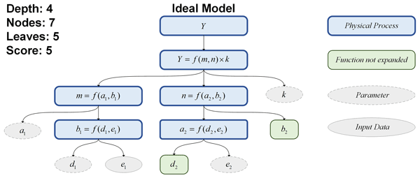
Figure 1A conceptual diagram of the Tree-Based Model Complexity Scoring (TBMCS) method. The root node is the target variable to be predicted (Y). The node will continue branching for each term in the equation if the term is further modeled using another equation or sub-model. The branching criteria for nodes follow the rules described in the text above.
2.5 The Tree-Based Model Complexity Scoring (TBMCS) method
To quantitatively assess the relationship between model performance and model complexity, we introduce a tree-based framework to evaluate process complexity and derive model complexity (Fig. 1). The assessment is based on multiple sources, including previous model intercomparison studies (Guo et al., 2024), official model documentation, available model code or technical implementation details (Sutanudjaja et al., 2018; Tang et al., 2006; Liang et al., 1994; Pokhrel et al., 2014; Oleson et al., 2010; Schaphoff et al., 2018; Burek et al., 2020; Hanasaki et al., 2008; Stacke and Hagemann, 2021; Best et al., 2011; Yokohata et al., 2020; Guimberteau et al., 2018; Müller Schmied et al., 2024), and supporting model publications (Müller Schmied et al., 2025; Telteu et al., 2021). These sources were cross-checked to identify how each model represents the four key snow-related processes considered in this study and to ensure a consistent basis for the subsequent process complexity assessment.
This framework characterizes structural differences in process representations using three tree properties: tree depth, number of nodes, and number of leaves. In this representation, the calculation of a variable Y at the root node (Fig. 1) is considered more complex when it involves a greater number of governing equations (nodes, blue boxes), input variables (leaves, grey boxes), and/or parameters (grey boxes with dashed outlines), or a deeper hierarchy of dependencies. These structural properties reflect the level of detail and explicitness in the representation of physical processes. More elaborate process representations may capture additional physical mechanisms and interactions, but greater structural complexity does not necessarily imply higher physical realism or better simulation performance.
To build such a tree, we start from a variable of interest and its mathematical equation at the root node. A node continues branching for each term in the equation if that term is further represented by an additional equation (or sub-model). Branching stops when one of the following criteria is met: (1) the term corresponds to an input dataset or parameter (Fig. 1, grey boxes); or (2) the term corresponds to a variable whose physical representation does not differ substantially among models or is already represented in another tree (Fig. 1, green boxes). By constructing such trees for the same target variable (e.g., Y in Fig. 1) and applying consistent branching criteria across different large-scale hydrological models, we establish a unified, quantitative, and measurable framework for evaluating the relative (rather than absolute; see Sect. 4) process complexity of snow-related processes.
After constructing the trees, the tree depth, number of nodes, and number of leaves are counted for each process in each model. Given the hierarchical structure governing a model's ability to simulate runoff characteristics, we assign weights of 0.6, 0.3, and 0.1 to tree depth, number of nodes, and number of leaves, respectively. This weighting scheme is intended to prioritize the hierarchical organization of process representation, while still accounting for the breadth of process formulation reflected by nodes and leaves. The weighted components are then summed to derive the process complexity value for each process, which is further aggregated across the four key processes to obtain the overall model complexity.
The weights assigned to tree depth, nodes, and leaves involve some methodological judgment and may influence the resulting complexity scores. To assess the sensitivity of the relative model rankings, we tested 12 alternative weighting schemes (Appendix Table C2). Schemes S1–S7 retained the largest weight for tree depth, consistent with the emphasis on hierarchical dependencies in the TBMCS framework, whereas Schemes S8–S12 relaxed this constraint to examine a broader range of weight combinations. The model rankings remained nearly identical across all schemes: only DBH and JULES-W2 exchanged the second and third positions, while the positions of all other models remained unchanged (Appendix Fig. C1). These results indicate that the relative model ranking is robust to the weighting choices tested in this study. The stability of the rankings across tested weights supports the internal robustness of TBMCS, while independent validation of the complexity construct remains a subject for future work.
Finally, we evaluate the four key physical processes described in Sect. 2.4 by assigning each a process complexity value that reflects the difficulty of estimating snowfall (Psnow), interception (Pint), sublimation (Esnow), and snowmelt (M). The model complexity of each model is then defined as the sum of the process complexity values of these four key processes, providing a straightforward measure of the overall complexity of the model as well as its relative emphasis on individual processes.

Figure 2The process complexity of rainfall-snowfall partitioning. Each schematic diagram shows the tree for each model. The plotting order is arranged from the lowest to the highest score. The gray, blue, and green shaded areas represent snowfall obtained directly from the forcing data, estimated using a fixed single temperature threshold, and estimated using a segmented dual-temperature threshold, respectively.
2.6 Experiment design
To analyze the relationship between model complexity and model performance, we use the Pearson correlation coefficient (r) as the primary metric. The Pearson correlation coefficient rxy between two variables x and y is defined as:
where xi and yi are the values of the ith () observations of variables x and y, and and are their respective means. In this study, x represents the model complexity and y represents the model performance.
To further disentangle the effects of individual basin complexity factors (i.e., DEM, DEMstd, LAI, PFTh) on the relationship between model complexity and model performance, we apply partial correlation analysis. This method quantifies the association between two variables while controlling for the influence of a third variable, and is defined as:
where rxy⋅z denotes the partial correlation coefficient between variables x and y after controlling for factor z. In this study, we define x as model complexity, y as model performance in a given basin, and z as a specific basin complexity factor.
3.1 Quantification and Characterization of Model Complexity
We begin our analysis by quantifying the process complexity of rainfall–snowfall partitioning (Fig. 2). Rainfall–snowfall partitioning is a key process controlling the phase of precipitation reaching the land surface, and thus strongly influences snow accumulation, subsequent meltwater availability, and SMR generation. Air temperature is widely recognized as the primary indicator for distinguishing precipitation phase. From the perspective of process complexity, existing models generally represent this process in two ways: (1) directly using precipitation phase provided by the forcing data (grey shaded area in Fig. 2), or (2) explicitly applying an internal temperature-threshold-based rainfall–snowfall partitioning scheme. Among the 13 ISIMIP models, four (MATSIRO, H08, MIROC-INTEG-LAND, and ORCHIDEE-MICT) directly use precipitation phase from the forcing data.

Figure 3The process complexity of interception. Each schematic diagram shows the tree for each model. Since the H08 model does not include an interception module, it is therefore excluded from the scoring. The plotting order is arranged from the lowest to the highest score. Gray, blue, and green shaded areas denote interception directly linked to the parameter, with LAI effects, and with evaporation effects, respectively.
Under the TBMCS framework, the first approach is treated as having lower internal process complexity because the phase-partitioning calculation is not explicitly represented within the model structure itself. We note, however, that this does not imply that the forcing treatment of precipitation phase is necessarily simple. In some cases, the forcing-generation pipeline may itself involve substantial preprocessing complexity, which is not captured by the present framework. Therefore, the rainfall–snowfall partitioning score used here should be interpreted as a measure of internal model process representation, rather than of the full complexity of forcing generation. The remaining nine models employ a rainfall–snowfall partitioning scheme, which typically follows one of two formulations: a fixed single-temperature threshold (blue shaded area in Fig. 2) or a segmented dual-temperature threshold (green shaded area in Fig. 2).
The fixed single-temperature threshold method adopts a constant critical temperature to determine precipitation phase. When the air temperature falls below the threshold, precipitation is classified as snowfall; otherwise, it is rainfall. Models such as PCR-GLOBWB, DBH, LPJML, CWATM, JULES-W2, and WATERGAP2-2E apply this approach. In contrast, the dual-temperature threshold method employs two critical temperatures to represent a transitional range between rainfall and snowfall (e.g., VIC, CLM40, HYDROPY). Based on these structural differences, the process complexity for the rainfall–snowfall partitioning across the 13 models ranges from 0.7 to 1.9.

Figure 4The process complexity of sublimation. Each schematic diagram shows the tree for each model. The HYDROPY and PCR-GLOBWB models were excluded from the sublimation process scoring because they do not include a sublimation module. The plotting order is arranged from the lowest to the highest score. Gray, blue, and green shaded areas denote sublimation directly linked to a fixed parameter, accounting for a resistance parameter, and further parameterized surface resistance, respectively.
Following rainfall–snowfall partitioning, snow interception is the next key process that determines the fraction of snowfall retained within the canopy versus that reaching the ground. This process also influences the exchange of energy and mass between the forest canopy and the atmosphere, thereby altering the sub-canopy snow distribution. Among the 13 ISIMIP models, all except H08 include an explicit representation of interception (Fig. 3). Based on the TBMCS method, the process complexity range from 1.7 to 4.1. Most models share a similar three-layer tree depth, with differences primarily arising from the number of leaves (i.e., parameters). The magnitude of interception capacity is closely tied to vegetation representation, typically parameterized as a function of LAI (blue shading in Fig. 3). CWATM provides the simplest scheme, relying solely on a fixed coefficient (grey shading), whereas WATERGAP2-2E offers the most detailed formulation by accounting for vegetation, temperature, and evapotranspiration effects (green shading).
Notably, several models – including CWATM, HYDROPY, CLM40, LPJML, DBH, ORCHIDEE-MICT, and WATERGAP2-2E – do not distinguish precipitation phase in their interception parameterizations, applying a unified scheme for both rainfall and snowfall. In contrast, the remaining models employ separate parameterizations specifically for snow interception.
Snow sublimation is a major snow-loss process during the cold season and a key component of energy and mass exchanges between the cryosphere and the atmosphere. Among the evaluated models, all except HYDROPY and PCR-GLOBWB explicitly represent sublimation, yielding process complexity from 1.6 to 4.7. These representations can be grouped into two main types: (1) a fixed sublimation value, as in LPJML (grey shading in Fig. 4); and (2) formulations that estimate sublimation based on evapotranspiration, adopted by the other models. Most models share a three- to four-layer depth and account for the effects of vapor pressure deficit (VPD), surface resistance (Rsurf), and aerodynamic resistance (Rair) on sublimation (blue and green shading). More complex implementations explicitly model Rsurf (green shading), primarily by incorporating vegetation characteristics such as LAI, as evident in JULES-W2, DBH, CLM40, and CWATM. CWATM also includes a crop-specific sublimation factor when the underlying surface is cropland, resulting in the highest process complexity (4.7).

Figure 5The process complexity of melt. Each schematic diagram shows the tree for each model. The plotting order is arranged from the lowest to the highest score. Gray and blue shaded areas denote the degree-day factor model and the energy balance model, respectively.

Snowmelt, the process through which accumulated snow ablates, is the most critical determinant of runoff generation. Based on structural differences, existing snowmelt modules can be broadly classified into two categories: degree-day models (grey shading in Fig. 5) and energy-balance models (blue shading in Fig. 5). PCR-GLOBWB, LPJML, CWATM, HYDROPY, and WATERGAP2-2E employ the degree-day method, whereas H08, VIC, DBH, MATSIRO, MIROC-INTEG-LAND, ORCHIDEE-MICT, JULES-W2, and CLM40 use an energy-balance formulation.
Degree-day models estimate melt solely from a degree-day factor, producing relatively low process complexity (1.8–2.2). Differences nevertheless exist among these models depending on whether the degree-day factor is fixed or dynamic. For example, PCR-GLOBWB, LPJML, and WATERGAP2-2E employ fixed factors, whereas CWATM uses a dynamic factor incorporating rainfall intensity and seasonality. HYDROPY also uses a dynamic factor that increases linearly with the number of snowmelt days.
In comparison, energy-balance models exhibit substantially higher process complexity (5.2–6.1), as they compute snowmelt by explicitly resolving the snowpack energy budget, including longwave and shortwave radiation, sensible and latent heat fluxes, ground heat flux, and the latent heat of fusion. Shortwave radiation is particularly critical. H08 calculates vegetation shading directly using albedo, whereas models such as JULES-W2, DBH, and CLM40 employ the two-stream approximation (Sellers, 1985). CLM40 further enhances this representation by explicitly accounting for vegetation structure and type through parameters such as stem area index (SAI), leaf reflectance, and spectral transmittance across PFTs. Surface albedo is another major component; although snow albedo depends on snow age, melt stage, surface temperature, water content, and impurities, simpler models (e.g., VIC) represent only its decay with snow aging. In contrast, CLM40 includes solar zenith angle, impurities such as black carbon and dust, snow age, temperature, and spectral dependence, yielding a far more comprehensive treatment.
In summary, degree-day models offer simplicity and computational efficiency but rely on empirical assumptions, whereas energy-balance models provide a more physically realistic depiction of snowmelt at the cost of increased process complexity and data requirements.
We aggregated the process complexity scores of the four key physical processes for each model to derive the model complexity (Table 1). The results indicate that the three most complex models are CLM40, JULES-W2, and DBH (scores > 14), whereas the least complex are PCR-GLOBWB, HYDROPY, LPJML, and H08 (scores < 10). Unlike earlier approaches defining complexity solely by the number of fluxes and storages (Müller Schmied et al., 2025), our framework provides a more quantitative and structurally consistent assessment by considering not only the represented variables but also the number of physical formulations, their associated parameters and input datasets.
The largest contributions to model complexity and inter-model variance arise from the melt process (1.8–6.1), followed by sublimation (0–4.7), interception (0–4.1), and rainfall–snowfall partitioning (0.7–1.9). This pattern highlights that existing models place the greatest emphasis on melt processes, while snow-accumulation processes are represented less extensively. A category-level comparison further shows that LSMs generally exhibit higher complexity than GHMs and the DGVM, primarily due to their detailed energy-balance formulations within the melt modules.

Figure 6Relationship between model complexity and model performance. Panels (a–c) present Qsum, Qmax, and CTQ, respectively. The red line denotes the fitted regression. Point shapes indicate model categories: circles denote GHMs, squares denote LSMs, and triangles denote the DGVM. ALL, GHM, and LSM represent the Pearson correlation coefficients calculated using all models, global hydrological models, and land surface models, respectively.
3.2 Linkage between model complexity and model performance
Based on the established complexity metrics for each model, we subsequently examine the relationship between model complexity and performance, aiming to identify the runoff characteristics and basin conditions for which more detailed snow-process representations show stronger positive associations with simulation skill. In the main analysis, we use the full model ensemble to assess the overall relationship between model complexity and model performance. Figure 6 summarizes these relationships across the three runoff characteristics. The results show that for CTQ (Fig. 6c), model complexity exhibits a positive relationship with model performance (r=0.32), defined as the proportion of basins with acceptable bias (± 20 % for Qsum and Qmax, ± 5 d for CTQ across 1455 basins). In contrast, for Qsum and Qmax (Fig. 6a and b), model complexity shows little to no consistent influence on model performance (r=0.08, r = −0.14, respectively).

Figure 7Relationship between model complexity and model performance under different basin complexity scenarios. (a–c) show the relationship under low basin complexity and (d–f) show the relationship under high basin complexity. The red line denotes the fitted regression. Point shapes indicate model categories: circles denote GHMs, squares denote LSMs, and triangles denote the DGVM. ALL, GHM, and LSM represent the Pearson correlation coefficients calculated using all models, global hydrological models, and land surface models, respectively.
We then divided basins into high and low basin complexity groups using the median value of basin complexity as the threshold, aiming to test whether the relationship between model complexity and model performance differs under contrasting basin complexity conditions. Figure 7 shows that the complexity–performance relationship is metric dependent. For Qsum and Qmax, model complexity shows weak or inconsistent correlations with model performance under both low and high basin complexity. In contrast, although the correlation is not statistically significant, CTQ exhibits a relatively stronger positive association with model complexity than Qsum and Qmax, particularly under high basin complexity (r=0.35; Fig. 7f). This suggests that the potential benefit of increased model complexity may be more evident for runoff timing than for runoff magnitude, especially in more complex basin conditions.

Figure 8Relationships between model complexity and simulation performance for snowmelt runoff volume (Qsum), peak flow (Qmax), and centroid timing (CTQ), stratified by meteorological forcing and calibration status. Model complexity is the total complexity score of the four snow processes, and simulation performance is the proportion of basins with acceptable biases (± 20 % for Qsum and Qmax, ± 5 d for CTQ). The complete ensemble of 13 models is grouped separately by forcing dataset (GSWP3 or GSWP3-W5E5) and calibration status (Yes or No). Blue, orange, and green bars represent Qsum, Qmax, and CTQ, respectively. Numerical labels indicate correlation coefficients, and n denotes the number of models in each subgroup. Error bars represent 95 % percentile confidence intervals obtained from 10 000 paired model-level bootstrap resamples within each subgroup, excluding resamples with undefined correlation coefficients. Asterisks indicate P<0.05. These subgroup analyses are exploratory and do not isolate the independent effects of forcing or calibration.
Given that the evaluated models differ in forcing datasets and calibration status as well as in snow-process complexity, we conducted forcing-stratified and calibration-stratified sensitivity analyses and applied bootstrap resampling to assess the uncertainty of the correlation estimates (Fig. 8). The main directional result for CTQ is robust across these analyses: model complexity remains positively correlated with CTQ performance in both forcing subgroups and in both calibration subgroups. Although these subgroup comparisons cannot fully isolate the independent effects of forcing and calibration because of remaining differences in model structure, parameterization, composition, and sample size, they allow us to examine whether the complexity–performance relationships persist under more comparable conditions by stratifying the models according to forcing dataset and calibration status and quantifying the associated uncertainty through bootstrap resampling.
Within the GSWP3 subgroup, the correlations between model complexity and performance are positive for Qsum and CTQ (r=0.38 and 0.17, respectively) and close to zero for Qmax (r = −0.05). Within the GSWP3-W5E5 subgroup, the correlations are weakly negative for Qsum and Qmax (r = −0.22 and −0.20, respectively), whereas the positive correlation for CTQ is substantially stronger and statistically significant (r=0.81, P<0.05). GSWP3-W5E5 incorporates updated meteorological forcing compared with GSWP3 (Cucchi et al., 2020). The stronger CTQ correlation within this subgroup suggests that the relationship between snow-process complexity and model performance may vary with forcing conditions. However, because the subgroups also differ in model composition, this contrast cannot be attributed solely to differences in forcing quality.
Within the calibrated model subgroup, model complexity exhibits strong positive correlations with Qsum and Qmax performance (r=0.86 and 0.82, respectively), whereas the corresponding correlations are much weaker among models without reported calibration (r=0.22 and −0.02, respectively). These differences suggest that parameter calibration may influence the observed relationship between process complexity and runoff-magnitude performance. However, the effects of calibration cannot be fully separated from differences in model structure and parameterization. Moreover, the wide bootstrap confidence intervals, particularly for the calibrated subgroup comprising only five models, indicate considerable uncertainty in these correlation estimates.
The process-level analysis provides complementary support for the CTQ result. CTQ performance is positively correlated with interception, sublimation, and melt complexity (r=0.21, 0.22, and 0.28, respectively), whereas melt complexity is negatively correlated with Qsum and Qmax performance (r = −0.20 and −0.37, respectively; Appendix Fig. C2). Thus, the positive direction of the complexity–CTQ relationship is maintained across forcing conditions, calibration groups, and individual snow-process components, supporting its robustness within the evaluated ensemble. At the same time, the variation in correlation magnitude and bootstrap uncertainty demonstrates that this relationship is not governed by process complexity alone, but is also affected by forcing quality, calibration, model structure, parameterization, and the limited number of models in each subgroup. Accordingly, these results do not imply that more complex melt formulations are universally superior, consistent with previous comparisons of temperature-index and energy-balance approaches (Magnusson et al., 2015) and of uncalibrated GHMs and LSMs in snow-dominated basins (Beck et al., 2017).

Figure 9Influence of basin complexity factors on the relationship between model complexity and model performance. Panels (a–d) correspond to DEM, DEMstd, LAI, and PFTh, respectively. In each panel, the x axis (Q1–Q10) represents deciles of the corresponding basin complexity factor, from the 10th to the 100th percentile. The values shown in parentheses denote the median value of that factor within each decile. Each grid cell indicates the partial correlation coefficient, where red denotes a negative correlation and blue denotes a positive correlation.
Figure 9 further illustrates how individual basin complexity factors influence the relationship between model complexity and performance. The partial correlation results vary among basin factors and runoff characteristics. For Qsum and Qmax, the correlations are generally weak and show no consistent change across the complexity gradients. In comparison, we also find that, for CTQ, the relationship between model complexity and simulation performance generally becomes more positive from Q1 to Q5 with increasing DEM and DEMstd. This pattern is physically plausible because snowmelt timing in high-elevation and topographically heterogeneous basins is influenced by multiple interacting processes whose representation may benefit from greater model complexity. However, this pattern is less evident for LAI and PFTh and should therefore be interpreted as a factor specific tendency rather than a general or statistically established effect of increasing basin complexity.
For the apparent threshold-like patterns in the relationship between model complexity and CTQ performance, the correlation with model complexity reaches a local maximum at a PFTh of approximately 0.95 (Fig. 9d). Greater vegetation diversity can enhance canopy–snow interactions (Musselman et al., 2008), whereas the coexistence of multiple canopy–snow processes under more heterogeneous vegetation conditions may partly obscure the influence of model complexity. A similar local maximum is observed at a DEMstd of approximately 180.07 m (Fig. 9b), beyond which the correlation no longer increases. This pattern may reflect the increasing influence of other sources of uncertainty, including forcing errors, routing effects, and parameter uncertainty. However, the updated correlations are weaker and not statistically significant; these local maxima should therefore be interpreted as tentative turning points within the evaluated basins and models rather than as well-defined or universal thresholds. Similar patterns are also present for Qsum and Qmax. For example, when DEM reaches approximately 930.33 m, the correlation between model complexity and Qsum performance reaches a local maximum of 0.29 (Fig. 9a). Likewise, at an LAI of approximately 0.32, the correlation with Qmax performance reaches 0.26 (Fig. 9c). Although these relationships are also statistically nonsignificant, their magnitudes are comparable to those observed for CTQ, further indicating that the apparent turning points are exploratory and dependent on the runoff characteristic and basin condition. These findings suggest that model development should consider basin-specific surface conditions, while avoiding the interpretation of the identified values as definitive thresholds for increasing process complexity.
The association between model complexity and CTQ performance tends to become more positive as DEM and DEMstd increase from Q1 to Q5, corresponding to low-to-moderate basin complexity. This pattern is physically plausible because increasing elevation and topographic heterogeneity strengthen the effects of radiation, snow albedo, terrain exposure, and snow redistribution on melt timing (Ma et al., 2023; Ban et al., 2023; Seibert et al., 2021; Freudiger et al., 2017), potentially increasing the relevance of detailed process representations. However, the trend weakens beyond Q5, possibly because forcing, parameter, and routing uncertainties increasingly obscure the influence of snow-process complexity. Moreover, the updated CTQ correlations are moderate and statistically nonsignificant, with magnitudes comparable to several relationships for Qsum and Qmax. The result should therefore be interpreted as a tendency limited to low-to-moderate DEM and DEMstd conditions rather than a general benefit of increasing model complexity.

Figure 10Relationship between model complexity and model robustness. Panels (a–c) present Qsum, Qmax, and CTQ, respectively. The red and blue line represent the fitted regression for all models and LSMs. HH (high model complexity and high model robustness), HL (high complexity and low robustness), LH (low complexity and high robustness), and LL (low complexity and low robustness) are defined based on the median values of the corresponding x and y axis variables. Point shapes indicate model categories: circles for GHM, squares for LSM, and triangles for DGVM. ALL, GHM, and LSM represent the Pearson correlation coefficients calculated using all models, global hydrological models, and land surface models, respectively.
Finally, we extend these findings from a new perspective by examining the relationship between model complexity and model robustness (Fig. 10). Here, robustness is defined as a composite criterion of model performance, requiring both low bias and a strong ability to maintain accuracy under increasing basin complexity (see Sect. 2.3 for details). Based on the median values of model complexity and model robustness, the models are classified into four groups: high-complexity/high-robustness (HH), high-complexity/low-robustness (HL), low-complexity/high-robustness (LH), and low-complexity/low-robustness (LL). By incorporating this indicator, Fig. 10 complements Fig. 6 by moving beyond general accuracy and providing a more comprehensive assessment of model robustness across different basin conditions.
Model complexity shows contrasting relationships with model robustness across the three runoff characteristics (Fig. 10). The correlations are negative for Qsum and Qmax (r = −0.28 for both), whereas CTQ robustness remains positively correlated with model complexity (r=0.33). The coefficient for CTQ is therefore numerically higher and opposite in direction to those for Qsum and Qmax. This pattern is consistent with the positive complexity–performance relationship identified for CTQ and suggests that models with more detailed snow-process representations tend to maintain greater robustness in runoff-timing simulations. Although the relationship is not statistically significant and remains subject to uncertainty associated with the limited model ensemble, its positive direction supports a characteristic-dependent role of model complexity in SMR simulation.
Therefore, to evaluate the uncertainty of these relationships, we supplemented the Pearson correlations (r) with Spearman correlations (ρ) and paired model-level bootstrap resampling (Appendix Fig. C3). Pearson and Spearman produce the same correlation directions across all comparisons involving overall performance, low and high complexity basins, and model robustness. For example, both methods show positive relationships for CTQ performance across all basins (r=0.32 and ρ=0.21), under high basin complexity (r=0.35 and ρ=0.31), and for CTQ robustness (r=0.33 and ρ=0.21). In comparison, the corresponding relationships for Qmax remain negative. The bootstrap intervals are wide and include zero, indicating substantial uncertainty in the correlation magnitudes and statistical significance. Nevertheless, changing the correlation metric and applying bootstrap resampling do not reverse the principal directional patterns.
The leave-one-model-out (LOMO) analysis further evaluates sensitivity to model composition (Appendix Table C3). The CTQ correlations remain positive in all 13 iterations under both Pearson and Spearman methods, while the Qmax correlations retain their negative direction in all Pearson iterations and 12 of 13 Spearman iterations. For Qsum, the positive direction is retained in all Spearman iterations and 11 of 13 Pearson iterations, with the two sign changes occurring close to zero. Although the estimated correlation magnitudes vary with model composition, the supplementary analyses consistently preserve the characteristic-dependent directional patterns. In particular, the positive association between model complexity and CTQ performance remains evident across correlation methods and all LOMO subsets, demonstrating that this central finding is not driven by any single model.
In addition, rainfall–snowfall partitioning differs from the other processes considered in TBMCS because some models diagnose precipitation phase internally, whereas others obtain it directly from forcing data. Consequently, the complexity embedded in forcing-side preprocessing may not be captured when TBMCS evaluates only model-internal process representations. We therefore excluded rainfall–snowfall partitioning in a sensitivity analysis to determine whether its treatment disproportionately affected the complexity–performance relationships. Its exclusion causes only minor changes in the Pearson correlations and does not alter their directions for Qsum, Qmax, or CTQ (Appendix Table C4). Together with the consistent results across correlation methods and LOMO subsets, this finding demonstrates that the positive association between model complexity and CTQ performance is neither driven by any single model nor dependent on the treatment of rainfall–snowfall partitioning in TBMCS.

Figure 11Cluster analysis of process complexity among different models. Columns correspond to Qsum, Qmax, and CTQ, while rows represent the four clusters: HH (high model complexity–high robustness), HL (high model complexity–low robustness), LH (low model complexity–high robustness), and LL (low model complexity–low robustness). Each radar plot illustrates the relative scores of four key process modules (Parti: partitioning, Interc: interception, Sublim: sublimation, and Melt) for the models within the corresponding cluster. Colored polygons denote individual models, and the thick black dashed line represents a reference model with maximum process complexity score of each process across all models, serving as a benchmark for comparison.
3.3 Physical Process Mechanisms and Targeted Model Optimization
To further interpret the findings presented above, we conducted a process-level analysis to link model complexity with robustness and to derive implications for future model development (Fig. 11). Models were classified into four quadrants (HH, HL, LH, LL) according to their overall model complexity and robustness (Fig. 10).
The radar plots reveal that models in the HH quadrant (high model complexity, high robustness) exhibit a more balanced distribution of complexity across key physical processes (Fig. 11a–c). This suggests that robust performance is not determined by model complexity alone, and may also depend on the specific configuration and interaction of individual process representations within the model. In contrast, models in the LL quadrant show more evident limitations in their process representations (Fig. 11i–l). For instance, H08 lacks an explicit canopy interception module, which may contribute to its relatively poor performance.
Models in the HL quadrant are characterized by high model complexity but low robustness. For example, although CLM40 incorporates a wide range of physical processes, its reliance on fixed default parameter values appears to limit performance and result in high bias (Yan et al., 2023). A comparison between HH and HL models indicates that their model complexity scores are not markedly different; thus, the divergence in performance is more likely driven by parameter choices, specific process formulations, and the strategies used to couple individual components.
By contrast, models in the LH quadrant demonstrate that satisfactory robustness can be achieved even with relatively modest model complexity. For example, CWATM is consistently classified as LH across all three runoff characteristics. Despite its relatively low overall complexity, this model maintains a relatively comprehensive representation of key hydrological processes. Notably, unlike other degree-day based models that use a fixed degree-day factor, CWATM adopts a more flexible melt formulation in which the degree-day factor is further adjusted according to rainfall intensity and snowmelt timing. This provides a more physically comprehensive representation of melt variability within a relatively simple model structure, illustrating that low complexity models can still achieve robust performance when their process formulations are carefully designed.

Figure 12Complexity of physical process representation in representative models. Each radar plot illustrates the relative scores of four key process modules (Parti: partitioning, Interc: interception, Sublim: sublimation, and Melt) for the models within the corresponding cluster. Colored polygons denote individual models, and the thick black dashed line represents the reference model with maximum process complexity score of each process across all models, serving as a benchmark for comparison.
To further investigate how individual physical process modules influence model performance, we selected three representative models along the linear relationship between model complexity and CTQ robustness identified in Fig. 10c. These models illustrate a gradient of model complexity and robustness (Fig. 12). The simple model H08 lacks key processes such as canopy interception, constraining its ability to realistically simulate SMR. In contrast, the medium complexity model CWATM incorporates all major hydrological processes but employs a simplified degree-day formulation for snowmelt estimation, which may limit its skill in capturing the timing of meltwater release. At the high complexity end, the DBH model includes a more comprehensive suite of physical processes and represents snowmelt using an energy-balance approach, which provides a more explicit representation of the physical realism of melt simulations. These model comparisons provide process-level clues consistent with the statistical patterns. Because the models also differ in parameters and other structures, the role of any individual formulation should be tested further through controlled comparisons.
This comparison highlights that although increasing complexity enables a more explicit representation of cryospheric processes, performance gains depend critically on whether the added complexity addresses key limitations – such as melt parameterization – rather than on structural complexity alone.
This study develops the TBMCS method, which for the first time systematically quantifies and compares the physical complexity of snow-related processes across 13 global hydrological and land surface models. Building on this, we conducted a comprehensive assessment across global 1455 basins to examine the relationship between model complexity and performance in simulating three key SMR characteristics (Qsum, Qmax, and CTQ), further revealing characteristic-dependent patterns in how model complexity relates to performance. Our findings provide new insights into the long-standing debate on where and to what extent the added complexity of models yields substantive performance gains. The primary findings are summarized as follows:
-
Substantial inter-model differences exist in the representation of physical process complexity, with total scores ranging from below 10 (e.g., PCR-GLOBWB, HYDROPY, LPJML, H08) to above 14 (e.g., CLM40, JULES-W2, DBH). The largest divergence arises from the snowmelt process (1.8–6.1), followed by sublimation (0–4.7), interception (0–4.1), and rainfall–snowfall partitioning (0.7–1.9), indicating that most of the complexity heterogeneity stems from different treatments of melt. For the different model categories, LSMs generally exhibit higher complexity than GHMs and DGVM, largely due to their inclusion of detailed energy balance schemes.
-
Model complexity shows characteristic-dependent relationships with model performance. Under high basin complexity, model complexity is positively correlated with CTQ performance (r=0.35), while the relationships for Qsum and Qmax remain weak. The correlations reach local maxima at PFTh = 0.95 and DEMstd = 180.07 m, indicating that basin conditions modulate the complexity–performance relationship. Importantly, within the model subgroup driven by the higher-quality GSWP3-W5E5 forcing dataset, the positive association between model complexity and CTQ performance is stronger (r=0.81, P<0.05), further indicating that the benefit of process complexity becomes clearer when forcing-related uncertainty is reduced. For model robustness, the correlations with complexity are positive for CTQ (r=0.33) and negative for Qsum and Qmax (r = −0.28 for both). Overall, these results suggest that greater snow-process complexity is more consistently associated with improved simulation of runoff timing than runoff magnitude.
-
Model performance is shaped less by complexity itself than by the systematic representation of key processes. The absence of key physical processes constrains model performance more severely than process simplification. DBH (high complexity–high robustness model) achieves high robustness through balanced and well-integrated process design, whereas H08 (low complexity–low robustness model) shows poor accuracy due to missing critical modules such as canopy interception. In addition, high complexity alone does not ensure robustness due to uncertainty of parameters (e.g., CLM40), whereas well-designed snowmelt modules enable even simple models to perform resiliently (e.g., CWATM).
This study provides a process-based assessment of how snow-process complexity relates to different dimensions of SMR simulation. Several methodological limitations and broader implications warrant further discussion:
-
First, TBMCS provides a relative measure of the structural complexity of selected snow-related processes rather than an absolute measure of overall model complexity or physical realism. The scores depend on methodological choices, including process selection, tree construction, weighting, and the availability of model documentation. Although the sensitivity analysis demonstrates stable model rankings across alternative weighting schemes, this does not independently validate the complexity framework. Furthermore, the current approach does not fully capture process coupling, feedbacks, or differences in mathematical formulations. Future work could refine these aspects and extend TBMCS to other hydrological processes.
-
Second, the complexity–performance relationships may be influenced by differences in forcing data, calibration strategies, model structures, and parameterizations. Although the stratified analyses reveal a recurring positive association between complexity and CTQ performance, the correlations vary across subgroups, and the bootstrap results indicate considerable uncertainty. These factors limit the independent attribution of performance differences to process complexity and the transferability of the findings to other model configurations, spatial scales, and hydrological conditions. Future experiments with consistent forcing and calibration protocols, particularly comparisons of alternative process representations within the same model, could help clarify these relationships.
-
Third, the different relationships across SMR characteristics may reflect their distinct physical controls. CTQ is closely related to snow accumulation and melt dynamics, which may benefit from more detailed snow-process representations. In contrast, Qsum and Qmax are additionally influenced by precipitation, water storage, runoff generation, and routing processes that are not fully represented in TBMCS. These differences may help explain the more consistent positive association between complexity and runoff-timing performance, although further controlled experiments are needed to test these mechanisms.
-
Finally, our findings suggest that future model development should focus on improving the representation of processes most relevant to the targeted hydrological characteristics, rather than increasing structural complexity uniformly. Recent advances in physical parameterization, uncertainty assessment, and catchment functional diversity (Cho et al., 2026; Puy et al., 2026; Ameli et al., 2026) collectively highlight the importance of process-oriented, uncertainty-aware, and basin-specific modeling strategies. Such approaches should balance physical process representation, predictive accuracy, observational constraints, and computational efficiency when developing and refining hydrological models.
Basin complexity is represented by the composite complexity index (CI) developed in Part 1 (Lei et al., 2026). The CI characterizes two major dimensions of environmental heterogeneity relevant to snowmelt runoff (SMR) simulation: topography and vegetation. Topographic complexity is represented by basin mean elevation (DEM) and the standard deviation of elevation within the basin (DEMstd). The former reflects altitudinal controls on temperature, precipitation phase, snow accumulation, and melt-energy conditions, whereas the latter represents terrain heterogeneity and its influence on the spatial variability of snowmelt and runoff generation. Vegetation complexity is represented by mean leaf area index (LAI) and plant functional type entropy (PFTh). These indicators characterize vegetation density and vegetation-type diversity, respectively, which influence canopy interception, shading, sublimation, and land-surface energy exchange.
To make the four indicators comparable, each indicator is normalized across all study basins:
where X represents one of the four basin-complexity indicators and Xmin and Xmax are its minimum and maximum values across the study basins. The CI is then calculated as the sum of the four normalized indicators:
All four components are assigned equal weights to provide a transparent and readily interpretable measure of basin complexity. Higher CI values indicate greater combined topographic and vegetation heterogeneity and, consequently, potentially more challenging conditions for SMR simulation. The CI is used here as a relative index for comparing environmental complexity among the study basins rather than as an absolute measure of hydrological complexity.
The robustness index (RI) characterizes how consistently a model performs across the basin complexity gradient (Lei et al., 2026). It combines two complementary attributes: performance stability, represented by the overall magnitude of model bias across CI levels, and adaptability, represented by the rate at which model bias changes with increasing CI.
All basins are first ranked by CI and divided into 10 groups containing approximately equal numbers of basins. For each group, the representative CI value (CIi) and model bias (Biasi) are calculated as the median CI and median bias, respectively. This stratification reduces the influence of uneven basin distributions along the CI gradient and gives comparable representation to different levels of basin complexity.
Performance stability is quantified using the stratified mean absolute bias (SMAB), calculated by integrating the absolute bias across adjacent CI groups:
where i denotes the index of the complexity groups, ranging from 1 to n−1, Biasi represents the median model bias within the ith complexity group, and CIi indicates the representative CI value of that group.
Adaptability is quantified using the slope (S) of the linear relationship between absolute model bias and CI:
where b is the regression intercept. A larger positive S indicates that model bias increases more rapidly with basin complexity and therefore represents weaker adaptability.
To enable comparison and integration, SMAB and S are separately normalized across the evaluated models to the range [0,1]. The normalized components are then combined using their Euclidean distance from the ideal condition (0,0):
A higher RI indicates that a model has both a lower overall bias and less performance degradation as basin complexity increases. RI is therefore interpreted as a relative, integrated measure of model robustness for inter-model comparison rather than as an absolute measure of model performance.

Figure C1Sensitivity of model complexity scores to alternative weighting schemes. Cell values indicate the complexity score of each model for a given weighting scheme. Red annotations indicate the rank change relative to the baseline scheme S1, where negative values denote an improved rank and positive values denote a lower rank. Schemes S1–S7 represent the main sensitivity experiments, whereas S8–S12 denote the stress-test schemes.

Figure C2Relationships between individual process complexity and model performance for key snowmelt runoff characteristics. Panels (a–d), (e–h), and (i–l) show the relationships between process complexity scores and model performance for Qsum, Qmax, and CTQ, respectively. Model performance is defined as the proportion of basins falling within the predefined acceptable bias ranges, i.e., ± 20 % for Qsum and Qmax, and ± 5 d for CTQ. Columns represent the four snow-related process modules considered in the TBMCS framework: rainfall–snowfall partitioning, interception, sublimation, and melt. Each point represents one model, with colors indicating model categories: dynamic global vegetation model (DGVM), global hydrological models (GHMs), and land surface models (LSMs). The black line denotes the linear regression fitted across all models, and the Pearson correlation coefficient (r) is shown in each panel.

Figure C3Comparison of Pearson and Spearman correlations between model complexity and snowmelt runoff performance and robustness, with bootstrap uncertainty estimates. Rows represent (a–d) runoff volume (Qsum), (e–h) peak flow (Qmax), and (i–l) centroid timing (CTQ). Columns show correlations with model performance across all basins, within low complexity basins, within high complexity basins, and with the robustness index, respectively, corresponding to Figs. 6, 7, and 10 in the manuscript. Model performance is defined as the proportion of basins with biases within ± 20 % for Qsum and Qmax and ± 5 d for CTQ. All correlations use the complete ensemble of 13 models. Blue and orange points indicate Pearson and Spearman coefficients, respectively; horizontal bars represent 95 % percentile confidence intervals obtained from 10 000 paired model-level bootstrap resamples, preserving the pairing between model complexity and performance or robustness. Red numbers denote the original-sample correlation coefficients, and bracketed values give the confidence limits. Vertical dashed lines indicate zero correlation. All displayed confidence intervals include zero.
Table C1Overview of models and data products considered in this study. Calibration status indicates whether explicit calibration information is available from the original model documentation or related model information. Models without explicit calibration information are grouped as uncalibrated in this study.

Table C2Alternative weighting schemes used in the sensitivity analysis of the TBMCS.

Table C3Leave-one-model-out (LOMO) sensitivity of the correlations between model complexity and overall snowmelt runoff performance across the complete ensemble of 13 models.

Table C4Sensitivity of the complexity–performance relationships to excluding rainfall–snowfall partitioning from TBMCS.

All data used in this study are available from public repositories: (a) ISIMIP model outputs from https://data.isimip.org/, last access: 19 November 2024; (b) GSHA (Yin et al., 2023; Yin et al., 2024) from https://doi.org/10.5281/zenodo.10433905. The code used in this study is available from the corresponding author upon reasonable request.
Conceptualization: PL, XL, HL. Investigation: XL, HL, PL. Data curation: XL, HL. Funding acquisition: PL. Methodology: XL, PL, HL, KZ. Visualization: XL, HL, KZ. Writing (initial): XL, HL, PL. Writing (review and editing): XL, HL, PL, KZ.
The contact author has declared that none of the authors has any competing interests.
Publisher's note: Copernicus Publications remains neutral with regard to jurisdictional claims made in the text, published maps, institutional affiliations, or any other geographical representation in this paper. The authors bear the ultimate responsibility for providing appropriate place names. Views expressed in the text are those of the authors and do not necessarily reflect the views of the publisher.
This study was supported by the National Key Research and Development Program of China (2022YFF0801303), the Beijing Nova Program (20230484302), the Beijing Nova Interdisciplinary Program (20240484647), the National Natural Science Foundation of China (42371481), and the Yunnan Provincial Science and Technology Project at Southwest United Graduate School (202302AO370012). The authors acknowledge valuable feedback from ISIMIP modelers Drs. Yusuke Satoh and Emmanouil Grillakis. We also thank Dr. Dashan Wang for insightful discussions related to this project.
This research has been supported by the National Key Research and Development Program of China (grant no. 2022YFF0801303), the Beijing Nova Program (grant no. 20230484302), the Beijing Nova Interdisciplinary Program (grant no. 20240484647), the National Natural Science Foundation of China (grant no. 42371481), and the Yunnan Provincial Science and Technology Project at Southwest United Graduate School (grant no. 202302AO370012).
This paper was edited by Xing Yuan and reviewed by three anonymous referees.
Ameli, A. A., Sharif, H., and McDonnell, J. J.: A Global Classification of Hydrologic Functional Diversity in Gauged and Ungauged Catchments, Nature Water, 4, 1271–1281, https://doi.org/10.1038/s44221-026-00699-6, 2026. a
Arkesteijn, L. and Pande, S.: On Hydrological Model Complexity, Its Geometrical Interpretations and Prediction Uncertainty: Uncertainty and Ill-Posedness in Hydrology, Water Resour. Res., 49, 7048–7063, https://doi.org/10.1002/wrcr.20529, 2013. a
Ban, Z., Xin, C., Fang, Y., Ma, X., Li, D., and Lettenmaier, D. P.: Snowmelt-Radiation Feedback Impact on Western U.S. Streamflow, Geophys. Res. Lett., 50, e2023GL105118, https://doi.org/10.1029/2023GL105118, 2023. a
Beck, H. E., van Dijk, A. I. J. M., de Roo, A., Dutra, E., Fink, G., Orth, R., and Schellekens, J.: Global evaluation of runoff from 10 state-of-the-art hydrological models, Hydrol. Earth Syst. Sci., 21, 2881–2903, https://doi.org/10.5194/hess-21-2881-2017, 2017. a
Best, M. J., Pryor, M., Clark, D. B., Rooney, G. G., Essery, R. L. H., Ménard, C. B., Edwards, J. M., Hendry, M. A., Porson, A., Gedney, N., Mercado, L. M., Sitch, S., Blyth, E., Boucher, O., Cox, P. M., Grimmond, C. S. B., and Harding, R. J.: The Joint UK Land Environment Simulator (JULES), model description – Part 1: Energy and water fluxes, Geosci. Model Dev., 4, 677–699, https://doi.org/10.5194/gmd-4-677-2011, 2011. a, b, c
Best, M. J., Abramowitz, G., Johnson, H. R., Pitman, A. J., Balsamo, G., Boone, A., Cuntz, M., Decharme, B., Dirmeyer, P. A., Dong, J., Ek, M., Guo, Z., Haverd, V., van den Hurk, B. J. J., Nearing, G. S., Pak, B., Peters-Lidard, C., Santanello, J. A., Stevens, L., and Vuichard, N.: The Plumbing of Land Surface Models: Benchmarking Model Performance, J. Hydrometeorol., 16, 1425–1442, https://doi.org/10.1175/JHM-D-14-0158.1, 2015. a
Beven, K.: Prophecy, Reality and Uncertainty in Distributed Hydrological Modelling, Adv. Water Resour., 16, 41–51, https://doi.org/10.1016/0309-1708(93)90028-E, 1993. a
Beven, K.: A Manifesto for the Equifinality Thesis, J. Hydrol., 320, 18–36, https://doi.org/10.1016/j.jhydrol.2005.07.007, 2006. a
Burek, P., Satoh, Y., Kahil, T., Tang, T., Greve, P., Smilovic, M., Guillaumot, L., Zhao, F., and Wada, Y.: Development of the Community Water Model (CWatM v1.04) – a high-resolution hydrological model for global and regional assessment of integrated water resources management, Geosci. Model Dev., 13, 3267–3298, https://doi.org/10.5194/gmd-13-3267-2020, 2020. a, b, c
Cayan, D. R., Dettinger, M. D., Kammerdiener, S. A., Caprio, J. M., and Peterson, D. H.: Changes in the Onset of Spring in the Western United States, B. Am. Meteorol. Soc., 82, 399–415, https://doi.org/10.1175/1520-0477(2001)082<0399:CITOOS>2.3.CO;2, 2001. a
Cho, E., Cho, E., Vuyovich, C., Li, B., and Jacobs, J. M.: Basin-scale evaluation of the Noah-MP land surface model for runoff and snow generation in the Missouri River Basin: insights and recommendations for parameterization scheme selection, Hydrol. Earth Syst. Sci., 30, 6359–6380, https://doi.org/10.5194/hess-30-6359-2026, 2026. a
Cucchi, M., Weedon, G. P., Amici, A., Bellouin, N., Lange, S., Müller Schmied, H., Hersbach, H., and Buontempo, C.: WFDE5: bias-adjusted ERA5 reanalysis data for impact studies, Earth Syst. Sci. Data, 12, 2097–2120, https://doi.org/10.5194/essd-12-2097-2020, 2020. a
Davenport, F. V., Herrera-Estrada, J. E., Burke, M., and Diffenbaugh, N. S.: Flood Size Increases Nonlinearly across the Western United States in Response to Lower Snow-precipitation Ratios, Water Resour. Res., 56, e2019WR025571, https://doi.org/10.1029/2019WR025571, 2020. a
David, C. H., Maidment, D. R., Niu, G.-Y., Yang, Z.-L., Habets, F., and Eijkhout, V.: River Network Routing on the NHDPlus Dataset, J. Hydrometeorol., 12, 913–934, https://doi.org/10.1175/2011JHM1345.1, 2011. a
Feng, D. and Gleason, C. J.: More Flow Upstream and Less Flow Downstream: The Changing Form and Function of Global Rivers, Science, 386, 1305–1311, https://doi.org/10.1126/science.adl5728, 2024. a
Freudiger, D., Kohn, I., Seibert, J., Stahl, K., and Weiler, M.: Snow Redistribution for the Hydrological Modeling of Alpine Catchments, WIREs Water, 4, e1232, https://doi.org/10.1002/wat2.1232, 2017. a
Guimberteau, M., Zhu, D., Maignan, F., Huang, Y., Yue, C., Dantec-Nédélec, S., Ottlé, C., Jornet-Puig, A., Bastos, A., Laurent, P., Goll, D., Bowring, S., Chang, J., Guenet, B., Tifafi, M., Peng, S., Krinner, G., Ducharne, A., Wang, F., Wang, T., Wang, X., Wang, Y., Yin, Z., Lauerwald, R., Joetzjer, E., Qiu, C., Kim, H., and Ciais, P.: ORCHIDEE-MICT (v8.4.1), a land surface model for the high latitudes: model description and validation, Geosci. Model Dev., 11, 121–163, https://doi.org/10.5194/gmd-11-121-2018, 2018. a, b, c
Guo, H., Hou, Y., Yang, Y., and Mcvicar, T. R.: Global Evaluation of Simulated High and Low Flows from 23 Macroscale Models, J. Hydrometeorol., 25, 425–443, https://doi.org/10.1175/JHM-D-23-0176.1, 2024. a, b
Hanasaki, N., Kanae, S., Oki, T., Masuda, K., Motoya, K., Shirakawa, N., Shen, Y., and Tanaka, K.: An integrated model for the assessment of global water resources – Part 1: Model description and input meteorological forcing, Hydrol. Earth Syst. Sci., 12, 1007–1025, https://doi.org/10.5194/hess-12-1007-2008, 2008. a, b, c
Hersbach, H., Bell, B., Berrisford, P., Hirahara, S., Horányi, A., Muñoz-Sabater, J., Nicolas, J., Peubey, C., Radu, R., Schepers, D., Simmons, A., Soci, C., Abdalla, S., Abellan, X., Balsamo, G., Bechtold, P., Biavati, G., Bidlot, J., Bonavita, M., De Chiara, G., Dahlgren, P., Dee, D., Diamantakis, M., Dragani, R., Flemming, J., Forbes, R., Fuentes, M., Geer, A., Haimberger, L., Healy, S., Hogan, R. J., Hólm, E., Janisková, M., Keeley, S., Laloyaux, P., Lopez, P., Lupu, C., Radnoti, G., de Rosnay, P., Rozum, I., Vamborg, F., Villaume, S., and Thépaut, J.-N.: The ERA5 Global Reanalysis, Q. J. Roy. Meteor. Soc., 146, 1999–2049, https://doi.org/10.1002/qj.3803, 2020. a
Horton, P., Schaefli, B., and Kauzlaric, M.: Why Do We Have so Many Different Hydrological Models? A Review Based on the Case of Switzerland, WIREs Water, 9, https://doi.org/10.1002/wat2.1574, 2022. a
Hou, Y., Guo, H., Yang, Y., and Liu, W.: Global Evaluation of Runoff Simulation from Climate, Hydrological and Land Surface Models, Water Resour. Res, 59, e2021WR031817, https://doi.org/10.1029/2021WR031817, 2023. a
Knoche, M., Fischer, C., Pohl, E., Krause, P., and Merz, R.: Combined Uncertainty of Hydrological Model Complexity and Satellite-Based Forcing Data Evaluated in Two Data-Scarce Semi-Arid Catchments in Ethiopia, J. Hydrol., 519, 2049–2066, https://doi.org/10.1016/j.jhydrol.2014.10.003, 2014. a
Lei, X., Lin, P., Zheng, H., Fei, W., Yin, Z., and Ren, H.: Systematic Analyses of the Meteorological Forcing and Process Parameterization Uncertainties in Modeling Runoff with Noah-MP for the Upper Brahmaputra River Basin, J. Hydrol., 653, 132686, https://doi.org/10.1016/j.jhydrol.2025.132686, 2025. a
Lei, X., Lin, H., Zheng, K., and Lin, P.: Process diagnostics of snowmelt runoff in global hydrological and land surface models – Part 1: A systematic evaluation across basins of increasing complexity, Hydrol. Earth Syst. Sci., 30, 5343–5372, https://doi.org/10.5194/hess-30-5343-2026, 2026. a, b, c, d, e, f
Liang, X., Lettenmaier, D. P., Wood, E. F., and Burges, S. J.: A Simple Hydrologically Based Model of Land Surface Water and Energy Fluxes for General Circulation Models, J. Geophys. Res.-Atmos., 99, 14415–14428, https://doi.org/10.1029/94JD00483, 1994. a, b, c
Lin, P., Pan, M., Beck, H. E., Yang, Y., Yamazaki, D., Frasson, R., David, C. H., Durand, M., Pavelsky, T. M., Allen, G. H., Gleason, C. J., and Wood, E. F.: Global Reconstruction of Naturalized River Flows at 2.94 Million Reaches, Water Resour. Res., 55, 6499–6516, https://doi.org/10.1029/2019WR025287, 2019. a
Ludwig, R., May, I., Turcotte, R., Vescovi, L., Braun, M., Cyr, J.-F., Fortin, L.-G., Chaumont, D., Biner, S., Chartier, I., Caya, D., and Mauser, W.: The role of hydrological model complexity and uncertainty in climate change impact assessment, Adv. Geosci., 21, 63–71, https://doi.org/10.5194/adgeo-21-63-2009, 2009. a
Ma, Y., Yao, T., Zhong, L., Wang, B., Xu, X., Hu, Z., Ma, W., Sun, F., Han, C., Li, M., Chen, X., Wang, J., Li, Y., Gu, L., Xie, Z., Liu, L., Sun, G., Wang, S., Zhou, D., Zuo, H., Xu, C., Liu, X., Wang, Y., and Wang, Z.: Comprehensive Study of Energy and Water Exchange over the Tibetan Plateau: A Review and Perspective: From GAME/Tibet and CAMP/Tibet to TORP, TPEORP, and TPEITORP, Earth-Sci. Rev., 237, 104312, https://doi.org/10.1016/j.earscirev.2023.104312, 2023. a
Magnusson, J., Wever, N., Essery, R., Helbig, N., Winstral, A., and Jonas, T.: Evaluating Snow Models with Varying Process Representations for Hydrological Applications, Water Resour. Res., 51, 2707–2723, https://doi.org/10.1002/2014WR016498, 2015. a
Merz, R., Miniussi, A., Basso, S., Petersen, K.-J., and Tarasova, L.: More Complex Is Not Necessarily Better in Large-Scale Hydrological Modeling: A Model Complexity Experiment across the Contiguous United States, B. Am. Meteorol. Soc., 103, E1947–E1967, https://doi.org/10.1175/BAMS-D-21-0284.1, 2022. a, b, c
Müller Schmied, H., Trautmann, T., Ackermann, S., Cáceres, D., Flörke, M., Gerdener, H., Kynast, E., Peiris, T. A., Schiebener, L., Schumacher, M., and Döll, P.: The global water resources and use model WaterGAP v2.2e: description and evaluation of modifications and new features, Geosci. Model Dev., 17, 8817–8852, https://doi.org/10.5194/gmd-17-8817-2024, 2024. a, b, c
Müller Schmied, H., Gosling, S. N., Garnsworthy, M., Müller, L., Telteu, C.-E., Ahmed, A. K., Andersen, L. S., Boulange, J., Burek, P., Chang, J., Chen, H., Gudmundsson, L., Grillakis, M., Guillaumot, L., Hanasaki, N., Koutroulis, A., Kumar, R., Leng, G., Liu, J., Liu, X., Menke, I., Mishra, V., Pokhrel, Y., Rakovec, O., Samaniego, L., Satoh, Y., Shah, H. L., Smilovic, M., Stacke, T., Sutanudjaja, E., Thiery, W., Tsilimigkras, A., Wada, Y., Wanders, N., and Yokohata, T.: Graphical representation of global water models, Geosci. Model Dev., 18, 2409–2425, https://doi.org/10.5194/gmd-18-2409-2025, 2025. a, b, c
Muñoz, R., Huggel, C., Drenkhan, F., Vis, M., and Viviroli, D.: Comparing Model Complexity for Glacio-Hydrological Simulation in the Data-Scarce Peruvian Andes, Journal of Hydrology: Regional Studies, 37, 100932, https://doi.org/10.1016/j.ejrh.2021.100932, 2021. a
Musselman, K. N., Molotch, N. P., and Brooks, P. D.: Effects of Vegetation on Snow Accumulation and Ablation in a Mid-latitude Sub-alpine Forest, Hydrol. Process., 22, 2767–2776, https://doi.org/10.1002/hyp.7050, 2008. a
Oleson, K. W., Lawrence, D. M., Flanner, M. G., Kluzek, E., Levis, S., Swenson, S. C., Thornton, E., Dai, A., Decker, M., Dickinson, R., Feddema, J., Heald, C. L., Lamarque, J.-F., Niu, G.-Y., Qian, T., Running, S., Sakaguchi, K., Slater, A., Stöckli, R., Wang, A., Yang, L., Zeng, X., and Zeng, X.: Technical Description of Version 4.0 of the Community Land Model (CLM), NCAR Technical Note NCAR/TN-478+STR, National Center for Atmospheric Research, Boulder, Colorado, USA, 257 pp., https://doi.org/10.5065/D6RR1W7M, 2010. a, b, c
Orth, R., Staudinger, M., Seneviratne, S. I., Seibert, J., and Zappa, M.: Does Model Performance Improve with Complexity? A Case Study with Three Hydrological Models, J. Hydrol., 523, 147–159, https://doi.org/10.1016/j.jhydrol.2015.01.044, 2015. a
Pokhrel, Y. N., Koirala, S., Kanae, S., and Oki, T.: Incorporation of Groundwater Pumping in a Global Land Surface Model with the Representation of Human Impacts, Water Resour. Res., https://doi.org/10.1002/2014WR015602, 2014. a, b, c
Puy, A., Aguiló-Rivera, C., Linga, S. N., Clarke, N., Richards, O., Flinders, S., and Melsen, L. A.: Fifty Years of Research Have Deepened Uncertainties in Global Irrigation Water Withdrawals, Nature Water, 4, 1343–1354, https://doi.org/10.1038/s44221-026-00710-0, 2026. a
Qin, Y., Abatzoglou, J. T., Siebert, S., Huning, L. S., AghaKouchak, A., Mankin, J. S., Hong, C., Tong, D., Davis, S. J., and Mueller, N. D.: Agricultural Risks from Changing Snowmelt, Nat. Clim. Change, 10, 459–465, https://doi.org/10.1038/s41558-020-0746-8, 2020. a
Reed, K. A., Medeiros, B., Jablonowski, C., Simpson, I. R., Voigt, A., and Wing, A. A.: Why Idealized Models Are More Important than Ever in Earth System Science, AGU Adv., 6, e2025AV001716, https://doi.org/10.1029/2025AV001716, 2025. a
Savenije, H. H. G.: Equifinality, a Blessing in Disguise?, Hydrol. Process., 15, 2835–2838, https://doi.org/10.1002/hyp.494, 2001. a
Schaphoff, S., von Bloh, W., Rammig, A., Thonicke, K., Biemans, H., Forkel, M., Gerten, D., Heinke, J., Jägermeyr, J., Knauer, J., Langerwisch, F., Lucht, W., Müller, C., Rolinski, S., and Waha, K.: LPJmL4 – a dynamic global vegetation model with managed land – Part 1: Model description, Geosci. Model Dev., 11, 1343–1375, https://doi.org/10.5194/gmd-11-1343-2018, 2018. a, b, c
Schoups, G., Van De Giesen, N. C., and Savenije, H. H. G.: Model Complexity Control for Hydrologic Prediction, Water Resour. Res., 44, 2008WR006836, https://doi.org/10.1029/2008WR006836, 2008. a
Seibert, J., Jenicek, M., Huss, M., Ewen, T., and Viviroli, D.: Snow and Ice in the Hydrosphere, in: Snow and Ice-Related Hazards, Risks, and Disasters, Elsevier, pp. 93–135, https://doi.org/10.1016/B978-0-12-817129-5.00010-X, 2021. a
Seiller, G., Anctil, F., and Perrin, C.: Multimodel evaluation of twenty lumped hydrological models under contrasted climate conditions, Hydrol. Earth Syst. Sci., 16, 1171–1189, https://doi.org/10.5194/hess-16-1171-2012, 2012. a
Sellers, P. J.: Canopy Reflectance, Photosynthesis and Transpiration, Int. J. Remote Sens., 6, 1335–1372, https://doi.org/10.1080/01431168508948283, 1985. a
Stacke, T. and Hagemann, S.: HydroPy (v1.0): a new global hydrology model written in Python, Geosci. Model Dev., 14, 7795–7816, https://doi.org/10.5194/gmd-14-7795-2021, 2021. a, b, c
Sutanudjaja, E. H., van Beek, R., Wanders, N., Wada, Y., Bosmans, J. H. C., Drost, N., van der Ent, R. J., de Graaf, I. E. M., Hoch, J. M., de Jong, K., Karssenberg, D., López López, P., Peßenteiner, S., Schmitz, O., Straatsma, M. W., Vannametee, E., Wisser, D., and Bierkens, M. F. P.: PCR-GLOBWB 2: a 5 arcmin global hydrological and water resources model, Geosci. Model Dev., 11, 2429–2453, https://doi.org/10.5194/gmd-11-2429-2018, 2018. a, b, c
Tang, Q., Oki, T., and Kanae, S.: A Distributed Biosphere Hydrological Model (Dbhm) for Large River Basin, Proc. Hydraul. Eng., 50, 37–42, https://doi.org/10.2208/prohe.50.37, 2006. a, b, c
Telteu, C.-E., Müller Schmied, H., Thiery, W., Leng, G., Burek, P., Liu, X., Boulange, J. E. S., Andersen, L. S., Grillakis, M., Gosling, S. N., Satoh, Y., Rakovec, O., Stacke, T., Chang, J., Wanders, N., Shah, H. L., Trautmann, T., Mao, G., Hanasaki, N., Koutroulis, A., Pokhrel, Y., Samaniego, L., Wada, Y., Mishra, V., Liu, J., Döll, P., Zhao, F., Gädeke, A., Rabin, S. S., and Herz, F.: Understanding each other's models: an introduction and a standard representation of 16 global water models to support intercomparison, improvement, and communication, Geosci. Model Dev., 14, 3843–3878, https://doi.org/10.5194/gmd-14-3843-2021, 2021. a, b
Valéry, A., Andréassian, V., and Perrin, C.: `As Simple as Possible but Not Simpler': What Is Useful in a Temperature-Based Snow-Accounting Routine? Part 1 – Comparison of Six Snow Accounting Routines on 380 Catchments, J. Hydrol., 517, 1166–1175, https://doi.org/10.1016/j.jhydrol.2014.04.059, 2014. a
Yan, H., Sun, N., Eldardiry, H., Thurber, T. B., Reed, P. M., Malek, K., Gupta, R., Kennedy, D., Swenson, S. C., Hou, Z., Cheng, Y., and Rice, J. S.: Large Ensemble Diagnostic Evaluation of Hydrologic Parameter Uncertainty in the Community Land Model Version 5 (CLM5), J. Adv. Model. Earth Sy., 15, e2022MS003312, https://doi.org/10.1029/2022MS003312, 2023. a
Yang, Y., Pan, M., Feng, D., Xiao, M., Dixon, T., Hartman, R., Shen, C., Song, Y., Sengupta, A., Delle Monache, L., and Ralph, F. M.: Improving streamflow simulation through machine learning-powered data integration and its potential for forecasting in the Western U.S., Hydrol. Earth Syst. Sci., 29, 5453–5476, https://doi.org/10.5194/hess-29-5453-2025, 2025. a
Yin, Z., Lin, P., Riggs, R., Allen, G. H., Lei, X., Zheng, Z., and Cai, S.: A Synthesis of Global Streamflow Characteristics, Hydrometeorology, and Catchment Attributes (GSHA) for Large Sample River-Centric Studies V1.1, Zenodo [data set], https://doi.org/10.5281/zenodo.10433905, 2023. a
Yin, Z., Lin, P., Riggs, R., Allen, G. H., Lei, X., Zheng, Z., and Cai, S.: A synthesis of Global Streamflow Characteristics, Hydrometeorology, and Catchment Attributes (GSHA) for large sample river-centric studies, Earth Syst. Sci. Data, 16, 1559–1587, https://doi.org/10.5194/essd-16-1559-2024, 2024. a, b, c
Yokohata, T., Kinoshita, T., Sakurai, G., Pokhrel, Y., Ito, A., Okada, M., Satoh, Y., Kato, E., Nitta, T., Fujimori, S., Felfelani, F., Masaki, Y., Iizumi, T., Nishimori, M., Hanasaki, N., Takahashi, K., Yamagata, Y., and Emori, S.: MIROC-INTEG-LAND version 1: a global biogeochemical land surface model with human water management, crop growth, and land-use change, Geosci. Model Dev., 13, 4713–4747, https://doi.org/10.5194/gmd-13-4713-2020, 2020. a, b, c
- Abstract
- Introduction
- Data and Methods
- Results
- Conclusions and Discussions
- Appendix A: Calculation of the basin complexity index
- Appendix B: Calculation of the model robustness index
- Appendix C
- Code and data availability
- Author contributions
- Competing interests
- Disclaimer
- Acknowledgements
- Financial support
- Review statement
- References
- Abstract
- Introduction
- Data and Methods
- Results
- Conclusions and Discussions
- Appendix A: Calculation of the basin complexity index
- Appendix B: Calculation of the model robustness index
- Appendix C
- Code and data availability
- Author contributions
- Competing interests
- Disclaimer
- Acknowledgements
- Financial support
- Review statement
- References