the Creative Commons Attribution 4.0 License.
the Creative Commons Attribution 4.0 License.
 | 06 Feb 2026
Image-based classification of stream stage to support ephemeral stream monitoring
Garrett McGurk
Anahita Jensen
Fred Martin Ralph
Morgan C. Levy
Intermittent rivers and ephemeral streams (IRES) constitute a large fraction of global river networks, provide important ecosystem services, and are increasing in number with climate change. Yet, observing stage and calculating discharge in IRES can be technologically and methodologically challenging. To address this problem, we develop a method to classify relative stage categories from field camera imagery, creating a time series of categorical flow states without the need for direct stage measurements. Specifically, we employ a Logistic Regression model to classify conditions of no water, low water levels, or high water levels for an ephemeral stream located in the upper Russian River watershed of California (US). We trained our algorithm using hourly field camera images from 2017–2023, and validated the image classifications with 15 min continuous stage observations. We then used image classifications to perform quality control on the continuous stage time series, which allowed us to identify when the stream was dry and when the sensor malfunctioned. Next, we compared the image classifications to publicly accessible modeled discharge from the NOAA National Water Model CONUS Retrospective Dataset. We discuss how in-situ monitoring including field cameras and the classification of field camera imagery, combined with surface meteorology and soil moisture observations, provides detailed hydrologic information important for understanding how climate affects IRES. Because the image classification approach is transferable to other ephemeral stream sites equipped only with field cameras, this methodology provides a low-cost option for observing relative stage on sparsely-measured IRES that can augment existing hydrologic modeling used by water managers.
- Article
(22740 KB) - Full-text XML
- BibTeX
- EndNote


Global climate models (GCMs) agree that California (CA) will experience warming with climate change (e.g., Hayhoe et al., 2004; Leung et al., 2004; Pierce et al., 2013; Polade et al., 2014), and will face significant and variable changes in hydroclimate (Dettinger, 2016; Persad et al., 2020). Annual average precipitation projections are less certain than those for temperature (Polade et al., 2017), with GCM projections from the Coupled Model Intercomparison Project (CMIP) Phase 6 showing a wide range of possible precipitation changes for CA. Li et al. (2022) narrowed these wide-ranging projections to estimate that CA precipitation will increase by 10 %–34 % and 7 %–32 % by the end of the 21st century, for northern and central-southern CA, respectively. Therein, climate change is expected to increase the proportion of annual precipitation delivered via atmospheric river (AR) storms, and extreme precipitation events from ARs are expected to become more common (Gershunov et al., 2019). Simultaneously, warmer temperatures, which correspond to increased evaporative demand, can lead to landscape drying and less runoff generation during dry periods (Underwood et al., 2018; Albano et al., 2022).
Effects of climate change on hydrology have already been observed in CA, including warmer spring temperatures leading to earlier spring runoff (Vicuna and Dracup, 2007). Similarly, snowline elevations in the Southern Cascade and Sierra Nevada mountains are already increasing and are expected to continue rising while snow accumulation decreases (Shulgina et al., 2023). At the same time, climate and land use change are expected to increase the likelihood of extreme flooding, which increases the probability of hydrologic failure at major dams in CA by 2100 (Mallakpour et al., 2019). These amplifications of temperature and precipitation variability impact water management, highlighting the need to develop tools to support water management adaptation (Mallakpour et al., 2019).
In particular, the prevalence of intermittent rivers and ephemeral streams (IRES) is expected to increase with climate change, and IRES remain vulnerable to anthropogenic threats (Acuña et al., 2014; Chiu et al., 2017; Gutiérrez-Jurado et al., 2019). IRES are defined as flowing waters that stop flowing or go dry at some point along their course (Datry et al., 2017) and they represent over 50 % of the world’s river network and global discharge (Acuña et al., 2014; Gutiérrez-Jurado et al., 2019). Flow initiation mechanisms for IRES include saturation-excess and infiltration-excess overland flow; interflow from saturated and unsaturated soils; and groundwater flow (Gutiérrez-Jurado et al., 2019). IRES flows support a variety of ecosystem processes and biodiversity by providing water to downstream river systems, nourishing riparian vegetation, and providing habitat for fisheries (Acuña et al., 2014). For example, IRES provide crucial habitats for the spawning and rearing of economically important species including coho salmon (Kerezsy et al., 2017). Fishes in IRES are threatened by habitat fragmentation due to climate change, river regulation, and water extraction (Kerezsy et al., 2017).
IRES and the downstream ecosystems they support are uniquely vulnerable to climate change. For example, Moidu et al. (2021) investigated the effect of climate variability on end-of-season (September or October) IRES wetting conditions for 25 streams in the lower Russian River watershed. They find that antecedent precipitation at seasonal to multiyear time scales strongly predicts end-of-season flow state alongside static landscape attributes such as geology, soil type (Gutiérrez-Jurado et al., 2019), and degree of weathering. Monitoring in Critical Zone Observatories (CZO) elsewhere shows that the effects of climate change on IRES can be localized, as exhibited by decreasing precipitation in two observatory catchments located in France and Mali leading to different outcomes: a decrease in flow and an increase in flow, respectively (Fovet et al., 2021). Furthermore, water-borne disease pathogens can be sensitive to river intermittency, and might be expected to change with climate change and human alterations to IRES catchments (Bertassello et al., 2021).
Due to the significant but relatively poorly understood contribution of IRES to downstream water systems – natural and managed – better understanding and managing of IRES networks is an important component of climate change resilience and adaptation in arid regions like the western US. For example, finding ways to keep water in the cooler, often-forested headwaters longer by increasing groundwater storage and maintaining IRES flow for longer periods of time benefits freshwater ecosystems, including valuable fisheries (Dettinger et al., 2023). Strategies for keeping water in headwater streams longer include “natural” options such as wetland restoration, beaver dam analogues, and forest thinning, as well as “managed” options such as Forecast Informed Reservoir Operations (FIRO; Dettinger et al., 2023), which uses weather and reservoir inflow forecasts to support more flexible reservoir operations (AMS, 2020). The functionality of any such strategy for climate change adaptation in IRES systems cannot be evaluated without comprehensive monitoring.
Problematically, observing IRES systems has historically been limited and challenging, especially because many IRES are in remote areas that may be difficult to access (Magand et al., 2020). In addition to inaccessibility, developing an in-situ monitoring network for stage and discharge on IRES is difficult because nascent gage networks may have less expertise, support, or funding compared to established national programs that generally focus on perennial streams (Vlah et al., 2024). There are also many environmental challenges to monitoring IRES, including turbulent flow, sediment, and debris flows following storms (Vlah et al., 2024). Estimating discharge from stage using a rating curve approach can be especially difficult for IRES (Vlah et al., 2024), which are often located in less accessible areas with less-developed channels. While comprehensive monitoring of IRES across a wide variety of watershed sizes and climates is important (Fovet et al., 2021), it is rarely achieved.
In the absence of comprehensive in-situ monitoring, low-cost methods for detection of IRES states (e.g., wet or dry conditions) using satellite remote sensing can be useful. For example, Tulbure et al. (2022) used Landsat-8 and Sentinel-2 to detect ephemeral floods in Australia's dryland Murray-Darling Basin and Fei et al. (2022) used Sentinel-1 and Digital Elevation Models to map alpine IRES in the Tibetan Plateau. While publicly-available satellite remote sensing can help map IRES in some instances, cloud cover and vegetation often obscure streams from view and the generally narrow water surface of IRES can be difficult to resolve.
Another low-cost method for determining IRES states is using simple sensors that record time series data to indicate the stream state. For example, a measure of high electrical conductivity indicates that a stream is wet and low (or zero) conductivity indicates that a stream is dry (Chapin et al., 2014). Observations of water occurrence from conductivity sensors have also been combined with time-lapse imagery and stage measurements to gain a broader understanding of the spatial and temporal characteristics of the stream network (Kaplan et al., 2019). Alternatively, stream temperature measurements have been used in combination with statistical models to determine the presence of water in several IRES in the northwest Great Basin desert, USA (Arismendi et al., 2017). Finally, observations of sound produced by rivers can be used as a proxy for stage (Osborne, 2022), and may present another scalable low-cost solution to IRES monitoring.
Citizen science approaches can also be used to obtain IRES data. For example, CrowdWater is a mobile phone application that enables installation of virtual staff (stream stage measurement) plates on streams to measure relative stage over time (Seibert et al., 2019). As of November 2023, CrowdWater had over 18 900 virtual staff plate contributions mainly on perennial streams, and over 19 000 temporary stream contributions. Users can determine the status of temporary streams using the following categories: “dry streambed”, “wet streambed”, “isolated pools”, “standing water”, “trickling water”, or “flowing water” (CrowdWater, 2023). Another citizen science effort is an app called DRYRivERS that asks users to identify the state of a river or stream as flowing, disconnected pools, or dry (Truchy et al., 2023). Nevertheless, data acquired from citizen science approaches has its limits (e.g., variable participation, data quality) and is not always usable for science or management applications.
Because in-situ measurement of IRES is frequently not possible, modeling approaches are useful. Durighetto and Botter (2021) used a precipitation-based empirical model calibrated on field survey data to create a time-lapse visualization of IRES streamflow state in the Rio Valfredda catchment in the Italian Alps. Forghanparast and Mohammadi (2022) used a long short-term memory (LSTM) model to predict streamflow in IRES in the Texas headwaters of the Colorado River. Similarly, many contemporary studies use deep learning algorithms trained with hydrologic observations to predict streamflow in IRES and perennial streams (Kratzert et al., 2019; Le et al., 2021; Feng et al., 2023).
In-situ image-based (i.e., field camera) approaches provide another method to observe and quantify water level in IRES. Image-based approaches can provide visually verifiable image data without disrupting the stream channel, and can be used with or without water level measurement equipment. Takagi et al. (1998) identified water levels from images by finding the interface between a slanted metal strip and its refracted reflection. More recently, field studies have identified water levels from field camera images based on the color contrast of the water-air interface using methods similar to Otsu (1979) that segment grayscale images based on their gray-level image histogram. Leduc et al. (2018) used a time-lapse camera and methods accounting for image quality issues to identify the stage and width of a stream in Alberta, Canada, finding that their image-based estimates generally agreed with daily stage measurements from a pressure transducer. Zhang et al. (2019) found that near-infrared imagery has greater contrast at the water-air interface even during inclement weather, making the water line easier to identify on processed images of the staff gage. Noto et al. (2022) used low-cost stage cameras and reference poles to estimate 30 min stage with minimal error at five IRES test sites in the Montecalvello catchment of Italy. Similarly, Birgand et al. (2022) used time-lapse images of a tidal creek with a dedicated, high-contrast target background to accurately measure stage using open-source software for water level measurement (Chapman et al., 2022). To estimate river discharge in Brazil, Rodrigues et al. (2025) apply a combination of Large-Scale Particle Image Velocimetry and maximum entropy estimation to smartphone videos. While they are successful in some cases, these methods require specific equipment that make them less suitable for widespread use, and it remains that the image segmentation methods required by most of these approaches (Otsu, 1979; Leduc et al., 2018; Zhang et al., 2019; Noto et al., 2022) can struggle to function when lighting conditions are poor.
Finally, machine learning and deep learning models have been successfully applied to field camera images to identify stage, velocity, and/or discharge primarily on perennial streams. For example, Tosi et al. (2020) calculated streamflow velocities on the Brenta and Tevere rivers in Italy using a machine learning algorithm that tracks features across consecutive site images. For stream sites with reliable cellular data coverage, a cloud-based computer vision stream gauging system can use short videos from a stereo camera to adaptively learn to estimate stage, surface velocity, and discharge (Hutley et al., 2023). Gupta et al. (2022) trained a deep convolutional neural network (CNN) model to recognize relative measures of streamflow using U.S. Geological Survey (USGS) timelapse camera photos from six non-IRES monitoring locations. They found that the CNN model performs almost as well as traditionally estimated streamflow reliant on manual discharge data. Windheuser et al. (2023) used deep neural network models trained on both images and time series data, including precipitation and USGS gage height, to predict flood stage for two rivers in Georgia (US), showing the strength of combining machine learning with other data sources. Using image processing and deep learning for streamflow prediction is an emerging field that has mainly focused on perennial streams. Gupta et al. (2022) and Noto et al. (2022) highlight the need to create algorithms focused on IRES.
Here, we explore whether visual features in daytime imagery are sufficient to reliably classify IRES flow states for monitoring purposes. This research is motivated by data limitations common to IRES networks, the increasing availability of low-cost field camera equipment and imagery, and scientific interest in improving IRES monitoring due to their unique ecological value and sensitivity to climate change. We first introduce our study area: a headwater stream in the upper Russian River watershed, CA. Then, we describe methods for using a combination of machine learning and field camera imagery to classify water levels on IRES. Lastly, we evaluate the performance of the image-trained machine learning model and demonstrate the value of the approach for monitoring and understanding IRES in California and elsewhere.
2.1 Study site and data
The Center for Western Weather and Water Extremes (CW3E) at the Scripps Institution of Oceanography installed a hydrologic and meteorological sensor network during the fall and summer of 2017 in the upper Russian River watershed, CA (Fig. A1; Sumargo et al., 2021; Ralph et al., 2022). This network supports a reservoir operations strategy called Forecast Informed Reservoir Operations (FIRO) at Lake Mendocino, an impounded reservoir used for drinking water, flood control, hydroelectric generation, and recreation (Jasperse et al., 2020). The upper Russian River watershed is a rain-dominated basin characterized by a variable Mediterranean climate with warm, dry summers and cool, wet winters where atmospheric rivers can result in heavy rainfall and flooding (Sumargo et al., 2021). The mountainous portion of the watershed that drains into Lake Mendocino is composed of Mesozoic Franciscan Formation bedrock and is a lightly-managed combination of shrub/scrub, forest (deciduous, evergreen, and mixed), and herbaceous land cover (USGS, 2023); in contrast, the alluvial valleys are largely cultivated or developed (Cardwell, 1965; USGS, 2023).
We focus our image classification exercise on imagery obtained at one of six continuous streamflow monitoring sites in the upper Russian River watershed (Fig. A1), located in the 7.05 km2 Perry Creek sub-watershed (Fig. 1). We also use a nearby surface meteorology site, Deerwood (DRW in Fig. 1). The Perry Creek watershed is primarily composed of Franciscan sandstone with steep slopes that are prone to landslides (Delattre and Rubin, 2020). Perry Creek is an ephemeral stream at the stream site (PEC), which is located in a narrow, steep gorge ∼20 m downstream from a ∼5 m tall waterfall (Fig. A2) and just upstream of Lake Mendocino. The PEC site was chosen for this study because it had potentially erroneous and noisy stage measurements relative to nearby sites, making the field camera imagery useful for quality control of stage data.
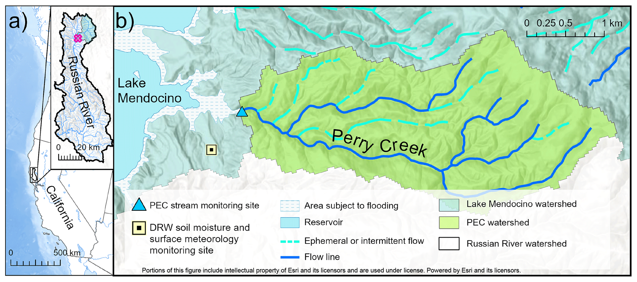
Figure 1The Perry Creek (PEC) study site in the upper Russian River’s Lake Mendocino watershed, California, US. (a) The location of the Russian River watershed (inset); the pink polygon shows the location of the study area shown in (b). (b) Perry Creek watershed and the Center for Western Weather and Water Extremes (CW3E) monitoring sites: the stream monitoring site at Perry Creek (PEC), the soil moisture and surface meteorology site at Deerwood (DRW), and associated hydrologic features (legend). Image data sources: CW3E and National Hydrography Dataset Plus (NHDPlus) High Resolution (Moore et al., 2019; Esri).
The PEC site is equipped with a staff plate and a stilling well containing a Solinst Levelogger (18 August 2017–11 October 2023) or HOBO MX2001-04-SS-S pressure transducer (11 October 2023–current) that record water levels at 15 min intervals (Fig. 2). There is missing data due to the inability to perform site maintenance because of the COVID-19 pandemic from 31 August 2020–24 February 2021. Atmospheric pressure from the DRW meteorological monitoring site was used to barometrically compensate stage at PEC measured by the Solinst Levelogger until the installation of a Solinst Barologger at PEC in January 2022 (Appendix A1; Figs. A3, A4). While DRW is not in the PEC watershed, it is less than 1 km from PEC and has continuous 2 min observations for the entire study period. We also use DRW’s observations of precipitation, relative humidity, temperature, and soil moisture (5, 10, 15, 20, 50, and 100 cm) for August 2017–November 2023. In October 2023, telemetry was installed at PEC, which includes a HOBO MX2001-04-SS-S pressure transducer and a HOBO MicroRX data logger, providing near real-time stage measurements. Prior to the installation of a HOBO telemetry system, stage data was downloaded directly from Solinst Leveloggers. The stilling well and staff plate configuration were not altered at the time of HOBO telemetry installation.
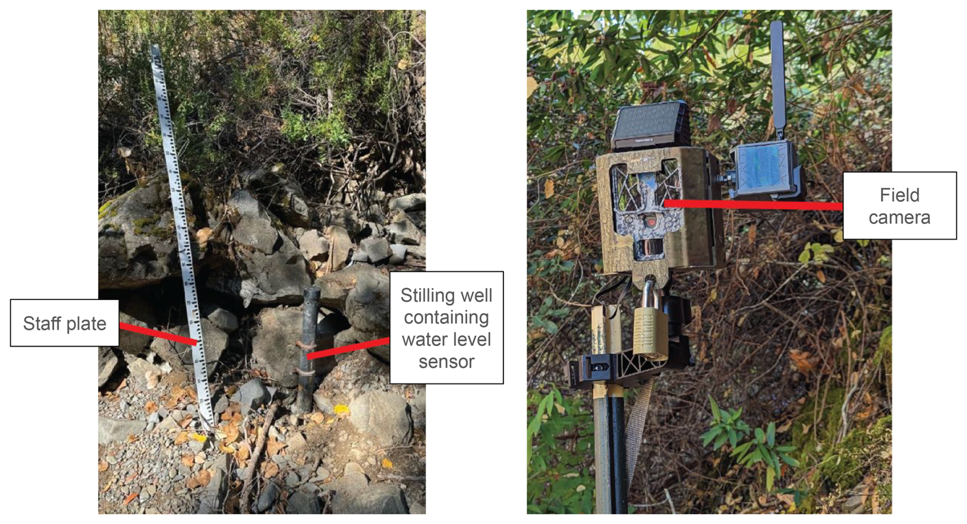
Figure 2Perry Creek (PEC) streamgage station equipment. The staff plate, stilling well, and water level sensor (left) are located at the side of the streambed; the field camera (right) is located across the stream channel, facing the staff plate.
The PEC site is also equipped with a trail field camera: a Wingscapes TimelapseCam Pro (6 November 2017–23 May 2018), Spypoint Link S Dark (27 January 2022–10 October 2023), or Force-S-Pro (11 October 2023–May 2024) which take photos of Perry Creek at hourly intervals (30 min intervals for 11 October 2023–May 2024; Fig. 2). The Wingscapes field camera only took photos from 05:00–18:00 Pacific Standard Time (PST; UTC−8), while the others took photos at all hours. In general, field equipment is susceptible to failure, including problems due to environmental exposure, such as water damage or reduced power generation from dirty solar panels. Field cameras at PEC malfunctioned frequently; the cameras were offline during June 2018–January 2022, June–July 2022, and March 2023–September 2023. The Wingscapes TimelapseCam Pro trail camera was prone to having its timestamp drift between field visits by as much as an hour, but we determined that these images were still likely representative of the approximate stage since flow states within an hour are sufficiently correlated.
Each field camera image captures the staff plate, streambed, and surrounding environmental features such as vegetation and rocks (Fig. A3). During occasional site maintenance, a handful of photos included people or were not focused on the streambed; we did not remove any of these from the dataset. Nighttime images are poorly illuminated, with the camera’s flash overexposing nearby vegetation and slightly illuminating the staff plate, making it difficult – if not impossible – to discern streambed conditions at night. Field camera images were downloaded manually during routine site maintenance once or twice each year. Site servicing also included clearing brush to prevent the camera from having an obstructed view of the stream.
Stream channel surveys and manual discharge measurements were collected from late 2017 through March 2024 at PEC. Manual discharge measurements were performed periodically, with a focus on capturing the full range of flow conditions. Manual discharge measurements were performed using a handheld flow meter (Pygmy, AA, or Hach MF Pro) and top-setting wading rod at discrete intervals along a measuring tape placed perpendicular to the streamflow (Turnipseed and Sauer, 2010). These discharge measurements were taken near the staff plate, with the staff plate level noted for data validation. As of water year 2024, there were 12 manual discharge measurements at PEC, which is not sufficient to create a stable rating curve for converting stage to discharge. Nevertheless, these measurements are still useful for beginning to constrain the magnitude and range of discharge values at PEC.
Finally, we use the NOAA National Water Model (NWM) Retrospective Version 2.1 dataset, a retrospective simulation from February 1979–December 2020 using version 2.1 of the NWM. This version uses land surface modeling based on the NOAH-MP Land Surface Model and meteorological inputs from the Office of Water Prediction's Analysis of Record for Calibration (NOAA, 2024a). We compare hourly NWM discharge from a segment that overlaps the location of PEC (Fig. A5; reach ID: 8268225) to PEC imagery, stage, and manual discharge data. Although the NWM was not calibrated using data from the PEC site, it was calibrated using data from the USGS East Fork Russian River streamgage (EFR in Fig. A1; Cosgrove et al., 2024), also located within the Lake Mendocino watershed. We chose the NWM for this comparison because it is a publicly-available dataset that is accessible to water managers and available for streams across the entire US. There is also precedent for using the NWM in combination with machine learning in the Russian River watershed as in Han and Morrison (2022) who used a LSTM to correct hourly NWM discharge predictions.
In summary, the following stage, discharge, and imagery data were available at PEC from 18 August 2017–30 November 2023: continuous 15 or 5 min stage observations for 91.3 % of the study period (with occasional missing data during site maintenance and prolonged missing data from 31 August 2020–24 February 2021), continuous hourly NWM-modeled discharge from August 2017–November 2020, 11 manual discharge measurements mainly from 2018, and 15 821 field camera images. Available field camera images documented the periods of November 2017–May 2018; February 2022–May 2022; August 2022–February 2023; and October 2023–November 2023.
2.2 Classifying water levels in field camera images
We used a supervised machine learning image classification approach to identify when there was no water, low water levels, high water levels, or an obstructed view at PEC using field camera images from August 2017–November 2023. The image classification approach involves multiple steps: image preparation; machine learning model selection, training, and evaluation; the development of measures to assess classification confidence; and a comparison of resulting classifications with observed stage, manual discharge measurements, modeled discharge, and hydrologic observations. This study develops an image classification method for PEC, which is transferable to any site with consistent streambed imagery.
2.2.1 Image preparation
We only used images taken between 09:00 and 16:00 PST because low-light images are more difficult to classify, even with a flash. To apply our method, all images were required to have the same dimensions. We selected a resolution of 1000×1200 pixels (Fig. 3a) because it was low enough to ensure that each image focused on the staff plate and streambed. Thus, the image size was determined by resolution constraints rather than through empirical or experimental testing. This cropping largely removed the effect of seasonal changes in vegetation that dominates the broader field of view and can make classification more difficult. Since the field cameras were reinstalled during some field visits at slightly different locations along the bank opposite the staff plate, there were four slightly different viewing angles of the streambed in the images. Cropping the images helped minimize the effect of these different angles. After cropping, we extracted the date the image was taken and the array of RGB pixel values from each image. The image preparation steps were performed using Python scripts with the sci-kit learn (Pedregosa et al., 2011c) and sci-kit image packages (Van der Walt et al., 2014).
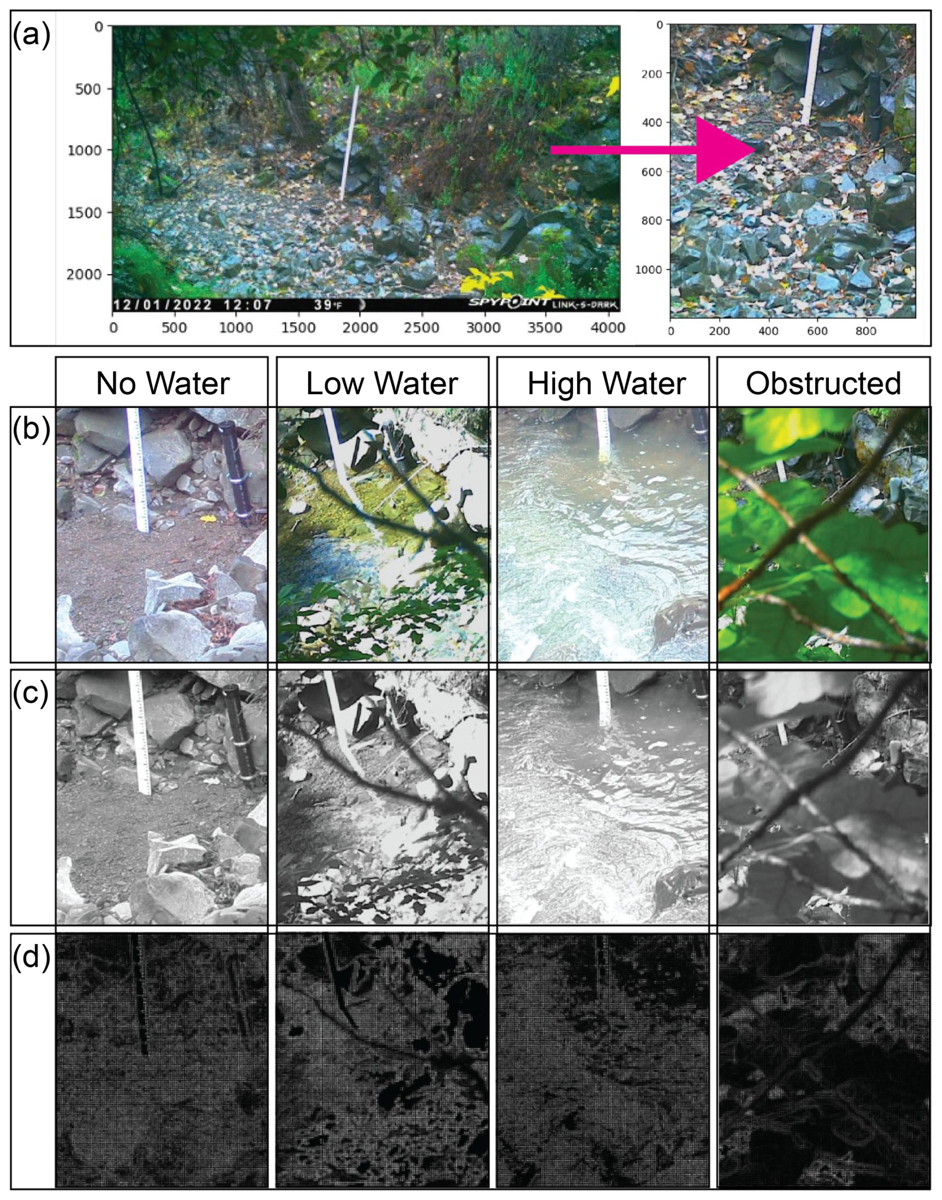
Figure 3Examples of imagery preparation steps for example field camera images. (a) Spypoint Link S Dark image for Perry Creek (PEC) from 1 December 2022, during a “no water” period; the image is cropped to center on the staff plate and set to a size of 1000×1200 pixels. (b) The four categories of labels for field camera images, showing each water level condition: “No Water”, “Low Water”, “High Water”, and “Obstructed”. (c) Examples of the grayscale conversion of (b). (d) The corresponding visualization of the histogram of oriented gradients (HOG) transformations of (c).
We then labeled a subset of images for supervised learning. Of the 4177 total PEC images taken from 09:00 to 16:00 PST during August 2017–November 2023, we manually labeled 537 images with four distinct categories: “no water”, “low water” level, “high water” level, and “obstructed” (Fig. 3b). We selected more than half of these 537 images using random selection and selected the remaining images manually using visual inspection to attain a representative sample across the four categories. This resulted in the purposeful selection of a labeled data set within which there were different numbers of images across categories, i.e., samples were “unbalanced” across categories. A small subset of images show stream states from similar time periods (i.e., dates and times are not regularly sampled), but because illumination and stream stage can vary by the hour even within the same day, we determined that the irregular time sampling should not bias model evaluation given the sample size. Because this study is limited to imagery from the study period, our analysis and modeling strictly reflect that period. However, if the variation in imagery and corresponding flow during the study period captures the seasonal and inter-annual variability typical of other years, then the selected images may be considered broadly representative. In our case, the study period includes the full range from wet to dry years and thus arguably captures this variability.
Our objective was to prioritize the classification of water presence or absence – a defining feature of IRES, by exploiting the visual differences in water surface texture and color for the “low” and “high” water categories. Firstly, we manually labeled images that consisted primarily of branches and leaves blocking the view of the streambed as “obstructed” even if we could discern the stream state. Images with some foliage present, but where the majority of the streambed was visible, were not labeled as “obstructed”, and were assigned a water level label. We then assigned the “low water” category to images with any presence of water, for which the water surface was characterized by low turbidity (i.e., clear water such that the staff plate is often reflected in the water) and the presence of little to no riffles. We assigned the “high water” category to images according to the presence of riffles, or even rapids, often with higher turbidity indicated by the water color being a light brown compared to the typically clear water. We assigned the “no water” category to images that lacked pooling or flowing water in the streambed. To maintain independence of categories, each of the 537 images were assigned only one category even if they were visually similar to multiple categories (e.g. relatively clear water with some ripples).
We processed the images to minimize the effects of different amounts of sunlight by converting the color images to black and white (Fig. 3c), increasing their contrast and flattening them using the histogram of oriented gradients (HOG) transformation (Lowe, 2004; Dalal and Triggs, 2005; Fig. 3d), and scaling their pixel values using the Python scikit-learn package (Pedregosa et al., 2011c). These transformations decreased color differences due to the time of day and season while making the water-air interface easier to distinguish.
2.2.2 Machine learning model
Within an individual model training and testing run, we randomly split the 537 labeled images into 70 % training data (375 images) and 30 % testing data (162 images). Figure 4 shows an example of this train-test split and demonstrates the unbalanced proportion of labeled images within different categories. We used the 375 training images to fit a logistic regression model using the Python scikit-learn package (Pedregosa et al., 2011c). The logistic regression model is a multinomial log-linear regression model typically used for categorical classification. We chose a multinomial classification model instead of a binomial classification model (i.e., for the presence or absence of water) in order to account for the “obstructed” view images, and to classify different flow states with distinct visual differences: “low water” versus “high water”. In this model, the classification of “high water”, “low water”, “no water”, or “obstructed” is determined by a linear combination of variables that represent the value and orientation of the pixels in each image.
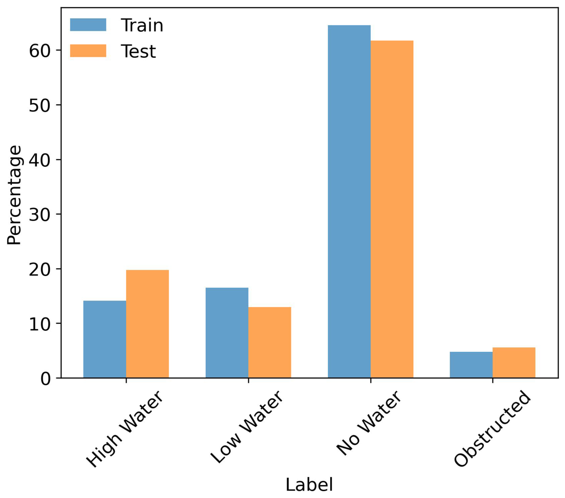
Figure 4Percentage (vertical axis) of labeled Perry Creek field camera images within each of the final model run's training (70 %) and testing (30 %) set split (colors) according to the label category (horizontal axis).
We selected the logistic regression model as the classification model in part due to its estimation of a probability for each categorical classification, where the estimated probability for a category is a function of the pixel values from the prepared image (see Sect. 2.2.1). We used a standard scikit-learn package implementation of a multinomial logistic regression model with L2 regularization (for mathematical details, see Pedregosa et al., 2011a). For model fitting, we used a cross-validation (CV) routine with six stratified “K” folds, meaning the training data were internally split into K (six) different training and validation sets that preserved the percentage of images within each labeled category.
We used 20 randomly-selected training and testing splits from the labeled image dataset to fit the model for six model “configurations”. Each configuration combined one of three different category weights and two different solvers, resulting in a total of 120 model training and testing runs. The three category weights were: no category weights; balanced category weights (due to our unbalanced data); and manually determined weights. We assigned manual weights to emphasize water presence categories (“high water” and “low water”) over “no water”, and gave the “obstructed” category a weight higher than “no water” (reflecting its smaller sample size) but lower than the water categories, given its lesser importance. The two solvers were lbfgs and newton-cg; a third solver, saga, was unable to converge at the selected maximum number of 300 iterations (and up to 1000 iterations). All remaining model parameters were set to the default scikit-learn package values (see Pedregosa et al., 2011b).
2.2.3 Model performance
Each of the n test-set image classifications falls into one of four categories: “no water”, “low water”, “high water”, or “obstructed”. For each category, the classification outcome is recorded as true positive (TP), false negative (FN), false positive (FP), or true negative (TN). Consider the “no water” category as an example. If a test-set image labeled as “no water” is correctly classified as “no water”, it is recorded as a TP; if misclassified as “low water”, “high water”, or “obstructed”, it is a FN. In contrast, if a different image labeled as anything other than “no water” is classified as “no water”, it is a FP; if classified correctly as any category other than “no water”, it is a TN. We used a confusion matrix to assess these outcomes.
To evaluate the performance of different model configurations, we computed key statistical metrics for the test set results across the 20 model runs within each of the six model configurations. Specifically, we calculated the mean, standard deviation, maximum, and minimum prediction accuracy (Eq. 1). To assess accuracy across categories, we computed the mean balanced accuracy (Eq. 2), defined as the average of recall (Eq. 3) for each classification category l=1, …, L. This approach ensures that model performance is not dominated by the majority category – “no water”. Next, we identified the best-performing model configuration based on the highest mean prediction accuracy and mean balanced accuracy across the six model configurations. Once selected, we used this model configuration to run the model with a fixed random seed for the train-test split and cross-validation routine, ensuring static parameterization. We refer to this as the “final model”. Then, this final model was used to classify the unlabeled images. Although this final model produces identical results for repeated runs on a given operating system, slight variability may occur across different operating systems due to differences in floating-point precision and parallel processing. To evaluate final model performance, we used the test set to calculate the prediction accuracy (Eq. 1), balanced accuracy (Eq. 2), recall (Eq. 3), precision (Eq. 4), and F1 score (Eq. 5; Pedregosa et al., 2011c).
2.2.4 Classification confidence
We developed confidence levels (i.e., high, moderate, and low) for classifications of “no water” and “any water”, where “any water” includes images classified as either “low water” or “high water”. To do this, we used test set images classified as “no water” or “any water” from the 20 model runs with the best-performing model configuration. From these data, we established confidence levels by comparing classification probability distributions to classification outcomes (TP, FN, FP, or TN) for the “no water” and “any water” categories. We defined “confidence levels” using probability value thresholds determined by visually and qualitatively assessing divergence in the distributions (boxplot medians and whiskers) of the estimated classification probabilities for “no water” and “any water” across the TP, FN, FP, and TN classification outcomes.
2.3 Comparing image classifications to observed and modeled hydrology
To understand how the classified imagery from the final model relates to stage and discharge times series, we compared our classified imagery to coinciding PEC stage, manual discharge measurements, and NWM discharge. This comparison is intended to help us understand to what extent classified field camera imagery can improve the often-limited and variable quality of observational and modeled stage and discharge data in IRES systems. We do this comparison graphically by overlaying time series plots of the barometrically compensated PEC stage with the classifications of concurrent, high-confidence image classifications. This time series plot allowed us to visualize discrepancies between image classifications and stage that enabled quality control of stage data (Appendix A2). The quality-controlled, barometrically compensated PEC stage data were then used for all subsequent analyses.
We compared the quality-controlled stage data to the NWM discharge and manual discharge measurements by overlaying each time series with corresponding high-confidence image classifications. We also use boxplots to visualize the ranges of stage and NWM discharge that correspond to each category of medium- and high-confidence image classifications. Using a scatter plot stratified by image classification category, we compared the PEC stage to NWM discharge and manual discharge measurements to determine the magnitude of discrepancy between data sources. For example, we calculated how often the observed stage at PEC was zero while the NWM predicted flow.
2.4 Environmental conditions
Finally, we compared our image classifications to surface meteorology and soil moisture observations from DRW to understand the concurrent and antecedent hydrologic conditions associated with “high water”, “low water”, and “no water” image classifications. We computed the daily total precipitation along with the daily mean temperature, daily mean relative humidity, and daily mean soil volumetric water content (VWC) at multiple depths (5, 10, 15, 20, 50, and 100 cm). We then graphically compared these daily observations to the time series of PEC stage that corresponded to high-confidence image classifications. Using scatter plots and linear regressions of those visualized data, we evaluated the relationship between 15 min stage observations stratified by medium- and high-confidence image classification and the following variables: the daily rolling mean soil VWC at 5 and 100 cm; the rolling sum precipitation at daily and monthly time scales; 2 min mean temperature; and 2 min mean relative humidity. We compared the 15 min stage to aggregated (rolling mean) values of soil moisture and precipitation to represent antecedent moisture conditions, but compared the same stage measurements to non-aggregated (2 min) temperature and relative humidity to represent concurrent weather conditions.
3.1 Model performance
The model configuration with the lbfgs solver and balanced category (class) weights performed best across the 20 model runs, with a mean prediction accuracy of 91 % and a mean balanced accuracy of 78 % (Table 1). In general, the mean balanced accuracy was lower than the mean prediction accuracy for each model configuration due to lower recall for the “obstructed” category compared to the other categories, resulting from a smaller training and test set size for the “obstructed” category. These performance metrics represent model performance evaluated on the testing set; we compare model predictions of flow states generated from both labeled and unlabeled images to stage and discharge measurements in Sect. 3.3.
Table 1Model configuration accuracy metrics across the six model configurations. Model configurations include the combination of solver and category weight options (rows), and accuracy metrics (columns) include the mean, standard deviation, maximum, and minimum for prediction accuracy, and mean balanced accuracy for the 20 model iterations (different random training and testing data splits) within each configuration. The first row shows the best-performing model configuration.
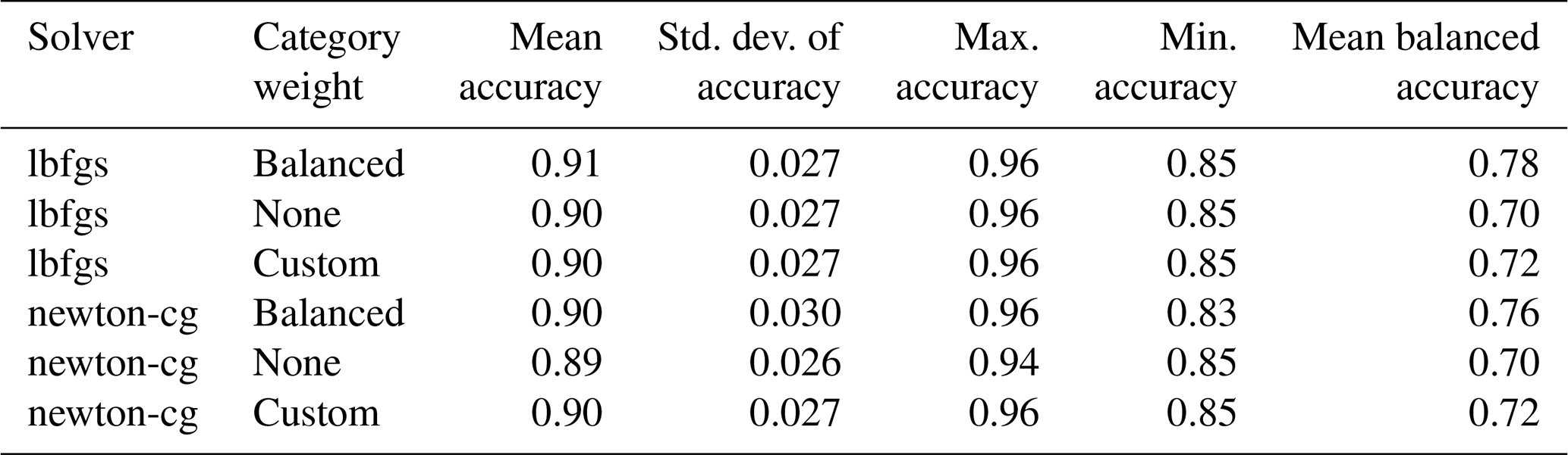
Within the 20 runs of the best-performing model configuration (lbfgs solver and balanced category weights), the minimum prediction accuracy was 85 % and the maximum prediction accuracy was 96 %, with a standard deviation of 2.7 % (Table 1). To illustrate the final model's performance within and across individual label categories, we used a confusion matrix (Fig. 5) to show classification outcome counts from the final model run. Classification outcomes across these 20 model runs are shown in parentheses in Fig. 5, which lists the range of counts of correct and incorrect classifications for individual labels. For example, “obstructed” images are misclassified as “high water” images a maximum of 7 times within any individual model run, but “high water” images never get classified as “obstructed”. Figure 5 also illustrates the data used to compute summary statistics of model performance. The most common incorrect classification within these 20 model runs was the classification of “low water” images as “no water”, which occurred in 2.8 % of all classifications. In addition, “obstructed” images were occasionally misclassified as either “high water” or “no water” (1.1 % and 1.8 % of these classifications, respectively). Due to the stream’s ephemerality, it is likely that there was in fact no water at PEC in the “obstructed” images misclassified as “no water”. Similarly, 2.4 % of image classifications were classifications of an incorrect water level (i.e., a “low water” classification when the image's label was “high water” and vice-versa). Because there is some overlap in image features that distinguish “low water” and “high water” images, incorrect water level magnitude classifications are expected, but do not detract from the utility of the model for prediction of IRES water presence or absence. The standard deviation of prediction accuracy across these 20 model runs was low (0.027, Table 1), indicating that any individual model run would produce similar image classifications when applied to the unlabeled images.
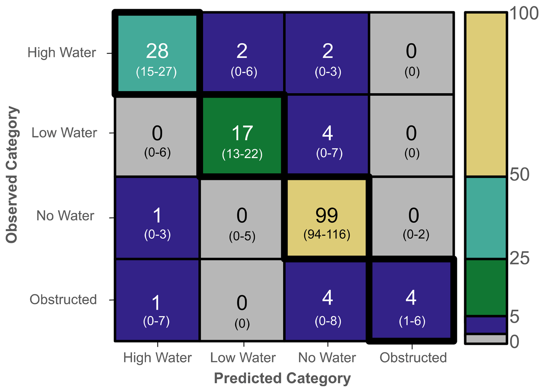
Figure 5Confusion matrix showing test set classification counts from the final model run. The matrix displays classification counts from the final model run (colors, centered text) and the range of classification counts across the 20 model runs (parentheses) using the best-performing model configuration – lbfgs solver and balanced category weights.
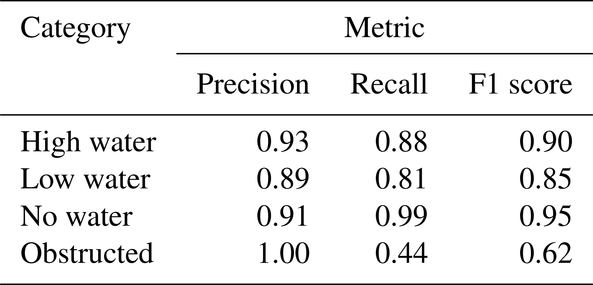
To run the final model, we used a static parameterization of the best-performing model configuration – lbfgs solver and balanced category weights. Table 2 shows accuracy metrics by image category for the final model run, showing greater than 0.80 for precision, recall, and F1 scores across all categories except for the recall and F1 scores for the “obstructed” category. Supplement Fig. A6 shows an example of test set output for the final model.
Table 2Precision, recall, and F1 scores for the final model run.
3.2 Classification confidence
We define levels of classification confidence based on assessment of the distributions (Fig. 6) of classification probabilities from the 20 model runs of the best-performing model configuration across TP, FN, FP, and TP classification outcomes. To assign levels of confidence, we chose thresholds in classification probability distributions that prioritized minimizing the risk of a false classification. To do so, we compared the distribution of true positive probabilities to false positive probabilities; we did not use false negative probabilities in the assessment of confidence because the probability of false negative outcomes is inherently much lower than the false positive probability for images with “no water” and “any water” labels (Fig. 6). We also did not use true negative probabilities in determining classification confidence because a true negative outcome represents any label other than the one considered.
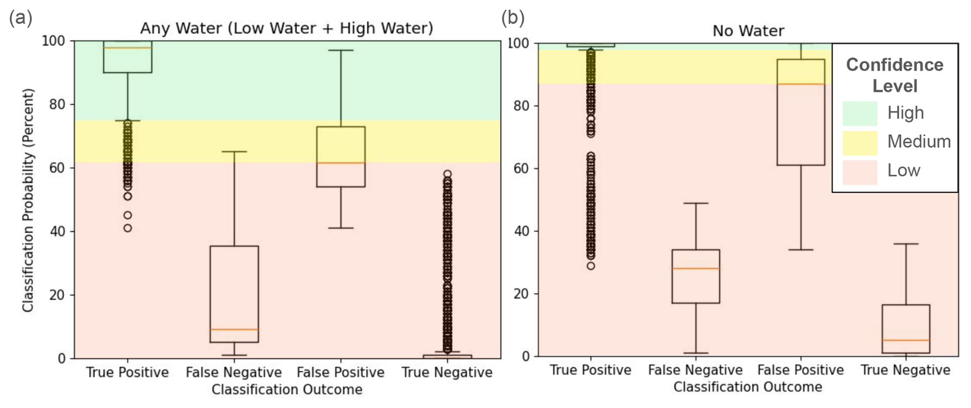
Figure 6The distribution of classification probabilities from the 20 runs of the best-performing model configuration evaluated on test set images. The panels show classification probabilities (vertical axis) across true positive, false negative, false positive, and true negative classification outcomes (horizontal axis) for: (a) “any water” (“low water” or “high water”) classifications and (b) “no water” classifications. The colors indicate the probability ranges used to assign high (green), medium (yellow), and low (red) confidence to image classifications. The boxplots show the interquartile range (IQR; box), median (orange line), the upper/lower quartile ±1.5 ⋅ IQR (whiskers), and outliers (points).
We assigned a “high” confidence level (Fig. 6, green) if the classification probability fell within the range of probabilities greater than the lower whisker for true positive classifications; this captures the full range of probabilities (excluding outliers) for true positive outcomes while not overlapping with the interquartile range for false positive outcomes for both the “no water” and “any water” categories. We assigned a “medium” confidence level (Fig. 6, yellow) if the classification probability fell within the range of probabilities less than or equal to the lower whisker for true positive classifications and greater than the median for false positive classifications; this captures some of the outlier probabilities for true positive outcomes, but recognizes that some probabilities in this range may be false positive classifications. Finally, we assigned a “low” confidence level (Fig. 6, red) if the classification probability was less than or equal to the median of false positive classifications. For the final model's classification of unlabeled images, we evaluated each image classification’s model-estimated probability according to these threshold values to provide categorical high, medium, and low confidence assignments for each classification. We subsequently used these confidence assignments, alongside their image classifications, to evaluate correspondence between water level classifications and modeled and observed water levels.
3.3 Comparing image classifications to observed and modeled hydrology
The medium and high confidence image classifications generally agreed with the PEC stage data. For example, a total of 94.6 % of images classified as “any water” corresponded to stage greater than zero, while 99.9 % of images classified as “no water” corresponded to a stage of zero. Low confidence image classifications did not agree nearly as well; 61.5 % of low confidence classifications identified “any water” when stage was greater than zero, and 56.7 % identified “no water” when stage was zero. This suggests that the model performed well on unlabeled imagery for high and medium confidence image classifications, but model performance decreased for low confidence image classifications.
The median stage for medium- and high-confidence image classifications for “high water” (27.1 cm) is greater than the median stage for images classified as “low water” (19.1 cm; Fig. 7a). In addition, the images classified as “high water” contain all but two occurrences of stage above the 99th percentile (46.1 cm, Table A1) at PEC (Fig. A7a). 75.1 % (63.2 %) of images classified as high (low) water level corresponded to stage above (below) the 90th percentile at PEC, which is equivalent to a stage of 21.5 cm (Table A1).
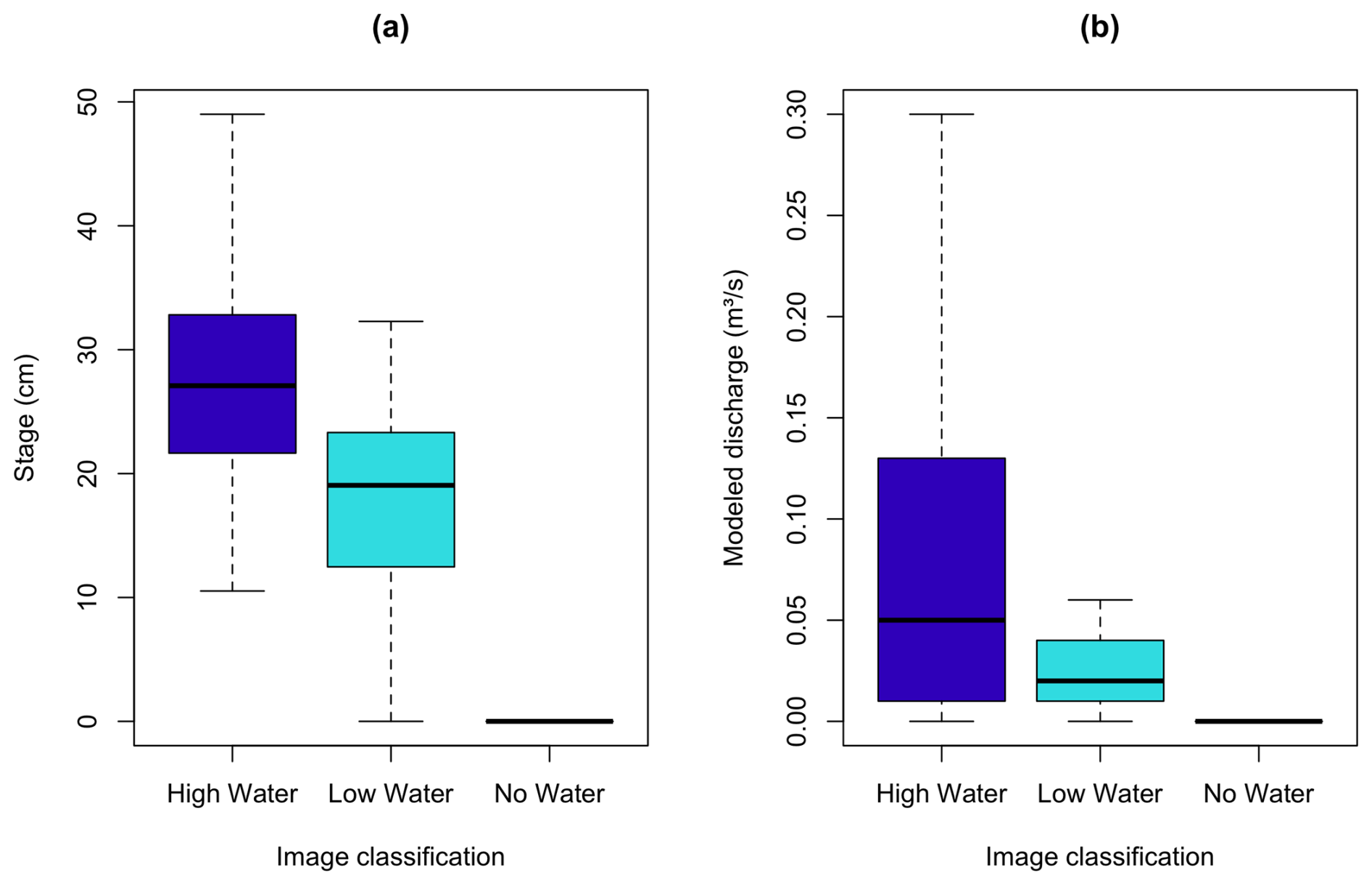
Figure 7Distribution of Perry Creek (PEC) stage and modeled discharge for medium- and high-confidence water level classifications. The boxplots show all values of stage (a) and modeled discharge (b) at PEC (vertical axis) corresponding to medium- and high-confidence (only) classifications of images as high, low, and no water (horizontal axis). The boxplots show the interquartile range (IQR; box), median (bold line), and the upper/lower quartile ±1.5 ⋅ IQR (whiskers); outliers were excluded from boxplots but not from the calculation of boxplot statistics (see Fig. A7 for boxplots with outliers).
We performed a similar comparison of classified images with modeled discharge data from August 2017–August 2020. The median modeled discharge for images classified as “high water” (0.05 m3 s−1) is greater than the median modeled discharge for images classified as “low water” (0.02 m3 s−1; Fig. 7b). In addition, the images classified as “high water” contain most of the extreme flow events, indicated by the “high water” classification containing almost all of the outliers (Fig. A7). 67.9 % (90.2 %) of images classified as high (low) water corresponded to modeled flow above (below) the 90th percentile (0.04 m3 s−1). All images classified as “no water” corresponded to flow less than the 80th percentile (0.02 m3 s−1), but approximately 18.2 % of images classified as “no water” have non-zero modeled discharge, albeit near-zero.
Comparison of image classifications to stage data is a diagnostic tool for quality assurance of observed stage data, which can be prone to sensor error, as shown for December 2022–February 2023 before (Fig. 8a) and after quality control (Fig. 8b). The final corrected and quality-controlled PEC stage time series (Fig. 9) is the product of standard quality control (i.e. removal of stage observations taken during sensor maintenance) and using image classifications to support quality control. Specifically, image classifications helped identify when the stage was zero for August 2017 to September 2023, supported the removal of erroneous data for most of January 2023, and revealed that stage observations are likely artificially low from late 2017 to early 2018. By comparing images classified as “no water” and the corresponding observed stage (visually), we determined that stage measurements oscillating near zero were noise instead of short-duration flow events; we then set those measurements to zero. An example of this is shown in Fig. 8a for December 2022 when the observed stage is less than zero with corresponding “no water” image classifications. Noisy data and stage measurements less than zero were an issue before installing the HOBO MX2001-04-SS-S pressure transducer and HOBO MicroRX data logger in October 2023; thus, the image classifications were useful in validating when the observed stage should be zero. Similarly, we used the stage time series and the image classifications of “high water” images to identify (visually) stage measurements that were erroneously low, and subsequently removed those measurements. For example, many of the images from January 2023 were classified as “high water”; however, the corresponding stage values were near zero or below zero (Fig. 8a). This indicated sensor measurement error that was likely related to turbulent flow conditions or debris from high flows; we flagged and removed almost a month of these data from the record (Fig. 8b). Stage data after 1 February 2023 in Figure 8 are uncertain as we do not have imagery available.
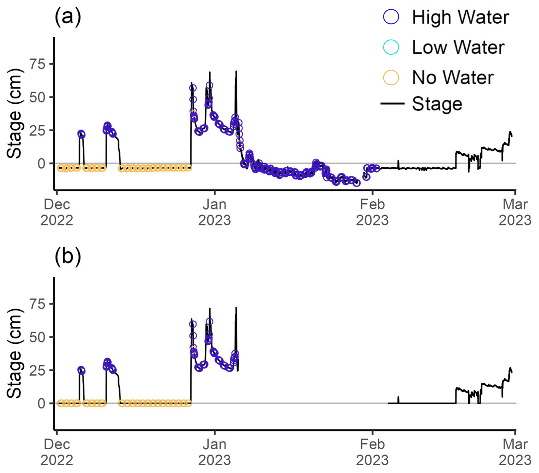
Figure 8Stage from the Perry Creek (PEC) site from December 2022–February 2023. No imagery was available after 1 February 2023. Stage values (black lines) are colored (points) by high-confidence image classifications (only). (a) Shows the time series before quality control, and (b) shows the time series after quality control.
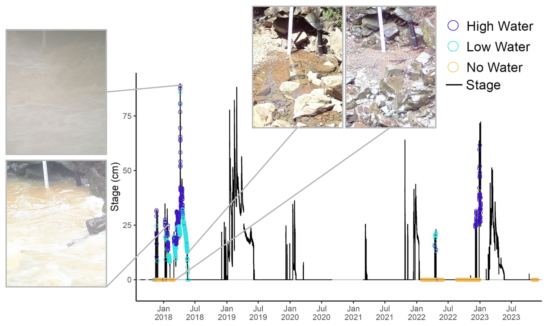
Figure 9Barometrically compensated and quality controlled stage from the Perry Creek (PEC) site from August 2017–November 2023. The time series shows PEC stage (vertical axis) across the full study period (horizontal axis) colored by concurrent high-confidence image classifications (colored points). Four example field camera images are shown. Field camera images were not available from 2019–2021.
Similarly, in late 2017 through early 2018, images were classified as “high water” while the observed stage was relatively low (Fig. 9). This identified a time period during which the stage sensor was likely pulled upwards in the stilling well sleeve due to debris catching on the exposed data cable, according to a subsequent site inspection. We chose not to remove the late 2017 through early 2018 stage data, but acknowledge that the stage is likely underestimated: the image classifications provided evidence that peak stage during this time may have been higher than recorded by the (compromised) stage sensor. This demonstrates the importance of critically evaluating observational data; in this case, image classifications reveal that several months of WY2018 are likely underestimated. For more details, see Appendix A2.
Instantaneous manual discharge measurements provide additional context (Figs. 10 and 11). There are several instances in which modeled discharge peaks correspond to PEC stage peaks (April 2018; Fig. 10). In contrast, modeled discharge is zero while the observed stage is greater than 10 cm for a total of 459 times (1.8 % of the times that modeled discharge and PEC stage overlap temporally); at these times, the mean observed stage is 19.8 cm, with a standard deviation of 5.1 cm. Observations of stage that exceed 10 cm while modeled discharge is zero, and for which we have image classifications, occur 83 times (5.2 % of the times where modeled discharge, PEC stage, and image classifications overlap temporally; Fig. 11). For example, from 18 January 2018 through 6 February 2018, image classifications show primarily “high water” and manual discharge measurements estimate flows of 0.167 and 0.368 m3 s−1, while the modeled discharge estimates 0 and 0.011 m3 s−1, respectively (Fig. 10). In contrast, during 19-21 March 2018, modeled discharge values were within 0.031 m3 s−1 of three contemporaneous manual discharge measurements (Fig. 10). There are also 3758 times (14.4 % of the times that modeled discharge and PEC stage overlap temporally) when the observed stage is zero while the modeled discharge is greater than zero; at these times, the mean discharge is 0.014 m3 s−1, with a standard deviation of 0.007 m3 s−1.
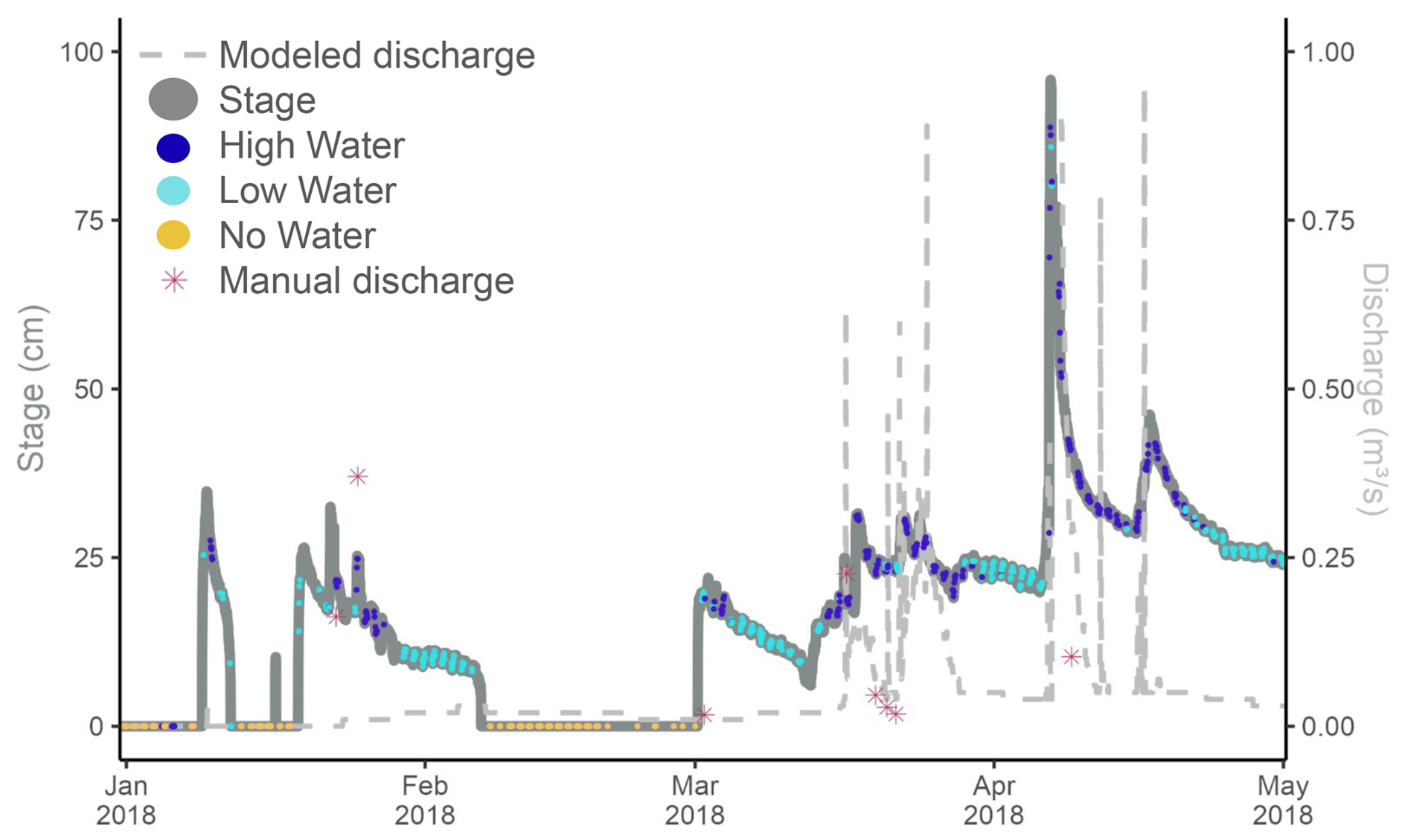
Figure 10Perry Creek (PEC) observed stage, instantaneous manual discharge measurements, and modeled discharge for January 2018 through April 2018. The PEC stage is colored by the high-confidence image classifications: “high water”, “low water”, or “no water”.
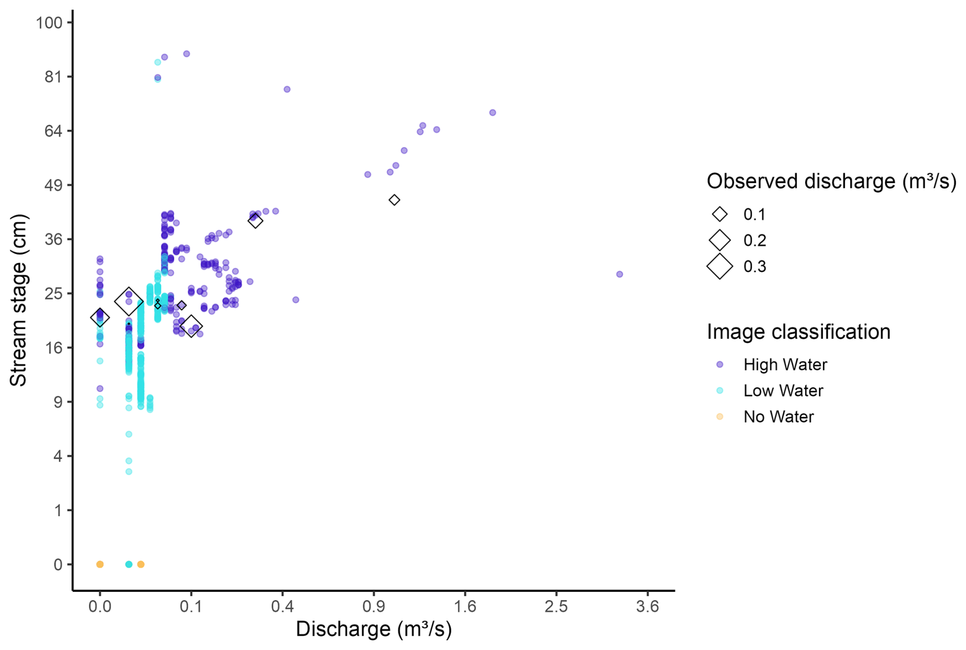
Figure 11Comparison between modeled discharge, manual discharge measurements, and observed stage at Perry Creek (PEC). Points show observations of stage (cm, vertical axis) and corresponding modeled discharge (m3 s−1, horizontal axis), according to the corresponding high-confidence image classification (color). The value of available manual discharge measurements (unfilled diamonds) corresponding to the observed stage and modeled discharge points are shown according to their magnitude (m3 s−1, diamond size).
Finally, while we do not have a sufficient number of manual discharge measurements to translate PEC stage to discharge across the full range of flow, the manual discharge measurements nevertheless provide some understanding of possible observation-based discharge values at PEC. The minimum observed discharge during periods with non-zero stage and discharge was 0.014 m3 s−1 on 19 April 2023, and the maximum observed discharge was 0.614 m3 s−1 on 6 March 2024. Photos and image classifications suggest that discharge can exceed this, but high flows remain unmeasured due to the site being unsafe to access during flows much higher than the 0.614 m3 s−1 measured on 6 March 2024. We gain some additional understanding of high discharge values at PEC by comparing modeled discharge and concurrent manual discharge measurements. This comparison (Fig. A9) indicates some agreement between measured and modeled discharge at moderate flows (< 0.283 m3 s−1), but poor agreement at higher flows (> 0.283 m3 s−1). Additionally, the longer time period modeled by the NWM (2000–2020, Fig. A10) suggests that our study period (2017–2020) does not capture the full range of peak flows at PEC.
3.4 Environmental conditions
In order to understand the hydrologic context of the image classifications and stage data, we evaluated temporal correspondence between stage and concurrent surface meteorology and soil moisture data (Figs. 12 and A8). In general, “high water” stage has a positive relationship with daily rolling sum precipitation (slope = 0.21, R2=0.41), 30 d rolling sum precipitation (slope = 0.16, R2=0.41), and 5 cm daily rolling mean soil VWC (slope = 126.36, R2=0.37). Similarly, “low water” stage is also positively related to these meteorological variables; the relationship is similar to that of “high water” for daily precipitation (slope = 0.47, R2=0.15) and less robust for 30 d precipitation (slope = 0.07, R2=0.2) and 5 cm soil VWC (slope = 29.74, R2=0.08). Notably, the R2 value for “high water” and 30 d precipitation indicates a stronger fit compared to the R2 value for “high water” and daily precipitation. There is also a slight positive relationship between “high water” stage and 100 cm daily soil VWC (slope = 22.65, R2=0.04).
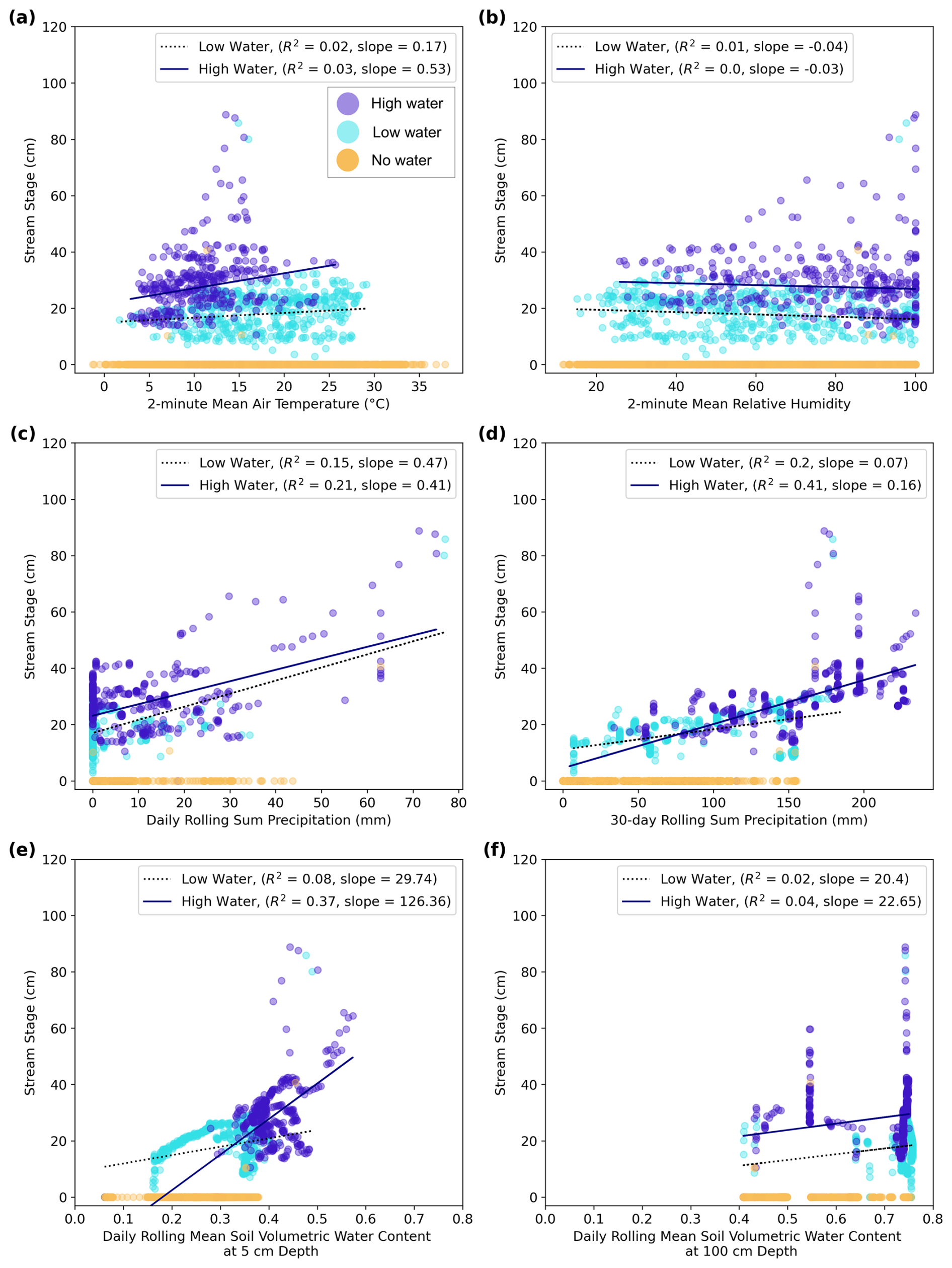
Figure 12Correspondence between Perry Creek (PEC) stage and concurrent surface meteorology and soil moisture data. PEC stage (cm, vertical axis) and its concurrent medium or high-confidence image classification (point color) compared to (horizontal axes): (a) 2 min mean air temperature, (b) 2 min mean relative humidity, (c) daily rolling sum precipitation, (d) 30 d rolling sum precipitation, and daily rolling mean soil volumetric water content at (e) 5 cm depth and (f) 100 cm depth. Linear regression estimates (lines, insets) summarize the relationship between stage and environmental data (a–f) for “low water” (dotted lines) and “high water” (solid lines) image classifications.
Stage does not have a clearly identifiable relationship with the other evaluated meteorological variables, although different stage values appear to occur within identifiable ranges of all the variables. All three image classification categories – “high water”, “low water”, and “no water” – occur for a wide range of temperatures, but there are no instances of water occurrence at temperatures greater than 30 °C (Fig. 12a). For relative humidity (RH) below 24 % there are only “no water” or “low water” classifications; for RH greater than 24 %, all three classifications are present but with an increasing number of “high water” classifications as RH approaches 100 % (Fig. 12b). Overall, maximum stage increases as RH increases, although stage was at times zero across the full range of RH values. Stage is only greater than zero when daily and 30 d rolling sum precipitation exceeds 45 and 160 mm, respectively (Fig. 12c–d), and stage is always zero when 30 d precipitation is at or near zero (Fig. 12d). The daily soil VWC regularly exceeds 0.7 at a soil depth of 100 cm (Fig. 12f), but rarely exceeds 0.5 at the shallower soil depth of 5 cm (Fig. 12e). While “high water” stage increases on average with increasing VWC at both 5 cm (slope = 126.36) and 100 cm (slope = 22.65) depths, stage measurements and their water level classification vary substantially across much of the range of VWC values. Even so, for 5 cm VWC, stage is zero when soil VWC is less than 0.15; only “low water” or “no water” classifications occur at soil VWC between 0.15–0.27; all classifications are present for soil water contents between 0.27–0.39; and stage is greater than zero when soil VWC is greater than 0.39. In summary, meteorological and soil moisture patterns are consistent with expected antecedent and coincident hydrology (stage) at this site, and also reflect expected patterns in the associated image classifications.
4.1 Image classification performance
We directly address the need to develop methods to observe stream conditions in IRES (Gupta et al., 2022; Noto et al., 2022) through the training and application of a simple logistic regression model for the classification of field camera imagery. While more complex machine learning model algorithms can sometimes provide more accurate image classifications, initial testing demonstrated that the logistic regression model performed better than standard implementations of other models, including image segmentation, clustering, and random forests. Our implementation prioritizes a simple, accurate, site-specific model that requires minimal manually-labeled training data. Even so, our overarching modeling workflow is transferable to other stream sites that have imagery with a consistent view of the streambed and only requires labeling a subset of site images as demonstrated in this study. Our method is optimal for detecting water presence in IRES, but is not intended to provide quantitative discharge estimates. For relative discharge estimates, a more complex model architecture may be helpful (Gupta et al., 2022; Goodling et al., 2025).
While our image classification method performed well, the method could be improved by further considering the time-dependence of flow states, especially in cases where stage data is either missing or not available. Since individual streamflow observations are related to each other at the 30 min or hourly time scale of the field camera images (i.e. if one image is classified as “no water”, the next image is more likely to also be classified as “no water”), this temporal correlation of flow states might be used to flag unlikely classifications and set them to a “low” confidence level. Precipitation and soil moisture data, in conjunction with the image classifications, could also provide additional quality control information even in the absence of stage or discharge measurements.
Furthermore, the present application includes only three categorical flow states which loosely correspond to quickflow (“high water”), baseflow or pooling (“low water”), and a dry streambed with no flow (“no water”). This is fitting for IRES as this classification approach prioritizes the presence or absence of water. Future work could expand the number of classified categories to include more water levels as in Seibert et al. (2019), Gupta et al. (2022), and Goodling et al. (2025). Specifically, our method could be expanded to detect IRES-relevant states including wet streambeds, isolated pools, standing water, trickling water, snow, or ice. Alternatively, models might be designed to estimate stage for images classified as “low water” or “high water” by building on methods for estimating stage on perennial streams, as in Leduc et al. (2018), but would need to address the problem of adverse lighting and turbulent flow conditions common to IRES.
One strength of the categorical image classification is that “low water” conditions include times of water presence in connected or disconnected pools, a distinct phase of IRES that supports aquatic life (Magand et al., 2020). Specifically, even well-adapted aquatic invertebrates living in IRES experience a steep decline in taxa richness with increasing flow intermittence (Stubbington et al., 2017). At PEC, the stage sensor is generally not exposed to water during pooling, so the stage is measured as 0 cm even when there may be water in nearby pools, meaning that the observed stage may not fully illustrate water presence. Thus, when cropping the images prior to classification, it was important to include most of the width of the streambed so that pooling in the streambed was visible. Further work could expand the “low water” category to separate low flow from pooling conditions. Discharge time series also do not capture the pooling phase of IRES because discharge is also zero at these times. Therefore, field camera images and image classification offer a way to observe the ecologically important “pooling” phase of IRES.
Regardless of the potential uses of field camera imagery, image quality and the reliability of field cameras will always be a challenge due to factors including inclement weather, shadows, and changes to IRES sites (i.e., high flows leading to debris accumulating in the channel). Pre-processing images helped to decrease the effect of variable lighting, and assigning classification confidence levels helped flag lower confidence classifications that may have been affected by image quality issues. Other studies have tackled this issue by pre-processing images with low image quality prior to classification. For example, Leduc et al. (2018) pre-processed images to account for image quality issues by removing images or adjusting identification methods in situations of inclement weather, shadows, or when rocks emerged from the streambed. Another issue is the difficulty of taking high quality images at night, even with a flash. Zhang et al. (2019) solved this problem by using an infrared camera, but regular cameras are often a better fit for remotely monitored sites. Finally, field cameras can often malfunction due to environmental exposure including extreme precipitation, humidity, and temperatures, making field cameras difficult to maintain.
For stream imaging generally, it is advantageous to choose a protected, stable, and fixed position for the field camera such that images are all taken with a full view of the streambed and from the same angle, which saves time during image pre-processing and classification. In this study, our method was complicated by four slightly different camera viewing angles. We minimized the effect of these changing viewing angles by cropping all images to focus on the staff plate and streambed. For locations with a time series of images with the same viewing angle, pre-processing would be less burdensome, and classification would likely improve because differences in images would only come from event evolution and not camera location.
4.2 National Water Model discharge at Perry Creek
We used NWM discharge estimates at the study site to demonstrate the use of image classifications to augment modeled discharge from a highly generalized streamflow prediction model, which the NWM represents. The observed differences between modeled discharge and stage are expected, particularly for small basins like that of PEC, since uncertainty in hydrologic models generally increases log-linearly as watershed area decreases (Carpenter and Georgakakos, 2004). In our case, modeled discharge values are for a stream segment that overlaps the PEC site (Fig. A5), so there is a difference in the spatial scales corresponding to stage and discharge measurements that may affect the comparison (Cosgrove et al., 2024; NOAA, 2024a). Specifically, the NWM’s representation of the PEC stream segment may have some overlap with Lake Mendocino during high lake levels, which could result in the representation of backflow from the lake as increased (observed) stage but with no corresponding increase in discharge. Additionally, much of the NWM’s PEC segment overlaps an area underlain by well-indurated Franciscan sandstone (Delattre and Rubin, 2020), which could induce higher discharge values along much of the Perry Creek segment relative to the location of the PEC site (see Appendix A3). Because the NWM is unable to resolve the detailed geology, steep slope, and groundwater-surface water interactions of this reach of Perry Creek, we would not expect the NWM to accurately reproduce flows at this particular site. While the NWM is generally relied upon to model discharge at larger scales (basin areas > 1000 km2), the modeled discharge estimates are nevertheless useful for representing the type of limited hydrologic information often available at less well-studied sites.
According to our comparisons, the NWM discharge misses or underestimates some short-duration, moderately-sized quickflow events (Fig. 10). Many “high-water” image classifications occur during January–February 2018, when the NWM shows little discharge. This is illustrated by two manual discharge measurements from January 2018 (Fig. 10), which record substantially higher flows at PEC than those simulated by the NWM. We hypothesize that the NWM struggles to represent early wet season flow processes in the steep slopes and low-infiltration soils of the PEC watershed. Later in the season, when soils in the PEC watershed are likely more saturated, the NWM discharge aligns more closely with PEC stage data and manual discharge measurements, suggesting that the NWM performs better under saturated conditions.
Additionally, at low stage and discharge levels, manual measurements of PEC discharge can be greater than those of modeled discharge (Fig. A9), and modeled low discharge appears stratified (Fig. 11). This is not surprising, as the NWM's physical process representation of low flow is not tailored to this site nor IRES systems in general. Low flows have been shown to be sensitive to the spatial scale of analysis and site-specific catchment characteristics, especially geology and soils (Chagas et al., 2024), which are not well represented in generalized models like the NWM. Conversely, at high stage levels, the few available manual measurements of discharge are less than corresponding modeled discharge (Fig. 11). Overall, our comparison makes clear that image classification in IRES benefits not only the quality of the in-stream observational record, but also stands to improve hydrologic model representations of IRES. Given the relatively uncertain but important contribution of IRES systems to downstream watershed flow regimes, better quantification of low flow components of inflows to heavily managed systems, like the Lake Mendocino watershed, would support water storage and delivery planning efforts (e.g., Jasperse et al., 2020).
4.3 Environmental conditions
DRW surface meteorology and soil moisture observations help establish the hydrologic context for the image classifications. These observations show the expected seasonal cycle of a Mediterranean climate with cool, wet winters and warm, dry summers, along with significant interannual variability in precipitation (Fig. A8). The ranges of meteorological and soil VWC values observed for different flow states (e.g., there only being “no water” classifications for temperatures > 30 °C) may provide helpful upper and lower bounds within which different flow conditions can be expected to occur in IRES. Nevertheless, a longer-term record of these data would be required to understand those bounds.
The comparison of soil VWC at 5 and 100 cm shows that high shallow soil moisture is a stronger predictor of water presence at PEC compared to deep soil moisture (Fig. 12e–f). The existence of “no water” image classifications across the full range of values for 100 cm VWC shows that deep soil moisture can be decoupled from the presence of water at PEC (Fig. 12f). In contrast, the shallow 5 cm VWC provides insight into the soil moisture conditions present during high water levels; “high water” image classifications are predominant when 5 cm VWC is greater than 0.39 (Fig. 12e). This, combined with our understanding of the geology of the PEC watershed, suggests that runoff generation at PEC is primarily driven by shallow subsurface flow and saturation- or infiltration-excess overland flow. With respect to low soil moisture conditions, stage was zero when 5 cm VWC was less than 0.15 (Fig. 12e), indicating that there may be a soil moisture threshold at which flow cannot occur at PEC.
Notably, there is considerable spatial variation in soil moisture observations, and the soil type at DRW is different from PEC (Soil Survey Staff at the Natural Resources Conservation Service at the US Department of Agriculture, 2024). Specifically, the soil hydrologic group at DRW is Group B, which indicates moderate infiltration rates, while the PEC watershed contains Groups C and D, which indicate slow or very slow infiltration rates, respectively (Soil Survey Staff at the Natural Resources Conservation Service at the US Department of Agriculture, 2024). This suggests that if soil moisture observations existed in the PEC watershed, the relationship between such observations and PEC stage could be different than our findings for DRW soil moisture and PEC stage. Based on the soil hydrologic group (Soil Survey Staff at the Natural Resources Conservation Service at the US Department of Agriculture, 2024), we hypothesize that for a given amount of precipitation, there would likely be more runoff generation in the PEC watershed compared to the area surrounding DRW. The different soil type at DRW is likely related to the different geology at DRW – the Ukiah Formation, an early Quaternary to Late Neogene continental basin deposit including conglomerate, silty sandstone, and clayey siltstone (Delattre and Rubin, 2020). In contrast, the PEC watershed’s steep slopes, landslide deposits, and fractured Franciscan Formation likely results in shallower and more unstable soils compared to soil in the rolling hills surrounding DRW. Confirmation of our understanding of the role of soils and geology in modulating the stage at PEC would require additional research that is beyond the scope of this work. Unique characteristics of the PEC site are further explored in Appendix A3.
4.4 Extensibility and potential applications
The classification model (see Data and Code Availability statement) is structured to ingest identically-sized images (with the streambed in the field of view) from any individual site’s field camera imagery collection, as long as a subset of images are labeled and sorted into folders that are named for each classification category. Due to there being multiple field camera angles at PEC, we cropped the images to focus on the stream channel and staff plate. However, images do not necessarily need to be cropped, and bank vegetation could potentially help the model predict flow states. For sites with consistent camera types and viewing angles, a useful exercise could be to find the optimal image resolution and cropping extent for feature recognition. In such an exercise, the cost of increased computing power for higher resolution images should be balanced with model performance.
Currently, the classification portion of the model code will work to classify any number of categories specified by the user, but the classification confidence portion is written specifically for the four categories from this work (“no water”, “low water”, “high water”, and “obstructed”). The code could be expanded to provide classification confidence values for additional and/or alternative categories by any user familiar with the Python programming language. In addition, a more objective strategy for evaluating classification confidence for other sites could be developed. Thus, the method as currently structured allows a user to create a time series of categorical flow states, sorted by confidence level, for any IRES site with similar timelapse field camera imagery (e.g., images from USGS Flow Photo Explorer; USGS, 2024) with or without stage sensors (see example application in Appendix A4 and Fig. A12). For sites without stage sensors, this method can estimate categorical flow states in IRES at low cost (Appendix A5). For sites with a stage sensor, image classification can support validation and quality control of stage data.
This work demonstrates that a simple machine learning algorithm can classify timelapse field camera images to identify no, low, or high water levels in IRES, providing a low-cost, transferable method for monitoring water occurrence in these sparsely observed systems. Given the prevalence of ungaged IRES, field cameras and image classification offer a practical approach to improving understanding of their role in climate-impacted freshwater systems. For example, the FIRO program at Lake Mendocino (Fig. A1) currently uses streamflow observations from EFR to inform reservoir inflow models. As climate change is expected to increase drying in IRES, unmonitored contributions from tributaries such as Perry Creek (Appendix A3) could affect reservoir storage. Thus, as the FIRO program expands, field cameras and image classification may offer a cost-effective approach to integrating information on the presence and magnitude of IRES contributions.
This approach can also support monitoring of critical habitats, including tributaries where salmon passage depends on streamflow connectivity threatened by drought and water diversions (see e.g., Scott River Watershed Council, 2025). Installing cameras at tributary confluences could inform targeted habitat restoration. More broadly, formally recognizing IRES as integral to river systems can incentivize monitoring and protect them from degradation due to climate change, mining, and urban development (Acuña et al., 2014). The 2023 exclusion of ephemeral streams from US Clean Water Act protections highlights the vulnerability of IRES and the importance of cost-effective monitoring approaches like ours for understanding the impacts and effectiveness of water management efforts.
We conclude by offering practical recommendations for implementing our method. Cameras should be installed along IRES reaches that are important for monitoring water management objectives (e.g., fish passage, drought contingency planning). Installations should be in stable locations with clear views of the streambed and minimal vegetation interference. Consistent camera types and viewing angles should be used, as they improve the robustness of time series and the effectiveness of classification. For the classification of categorical flow states, installation of a staff plate is not necessary, and basic image classification can be achieved with a limited number of labeled photos (on the order of 100 per site; see Appendix A4). Long-term maintenance budgets are also recommended to support sustained monitoring. Finally, this approach can be integrated with complementary methods (Gupta et al., 2022; Goodling et al., 2025) and deployed through accessible platforms such as the USGS Flow Photo Explorer (USGS, 2024) and the CrowdWater mobile application (SPOTTERON GmbH, 2025).
A1 Barometrically compensating stage data
Prior to the installation of barometric loggers in late 2021 or early 2022 at each CW3E stream site (Fig. A1), 2 min atmospheric pressure from nearby surface meteorology stations was used to barometrically compensate pressure measurements from the stage sensors. Each stream site was matched with a nearby surface meteorology site that was closest in elevation; thus, the Perry Creek stream site (PEC) was matched with the Deerwood (DRW) surface meteorology site. After the barometric loggers were installed at the stream sites, we were able to account for the difference in atmospheric pressure between the barometric logger location and the surface meteorology location by calculating the mean pressure difference for April 2022 through March 2023 (Figs. A3, A4).
The mean annual atmospheric pressure difference between DRW and PEC was 5.00 hPa. The minimum difference calculated at 15 min intervals was 3.30 hPa and the maximum difference was 7.10 hPa for April 2022 through March 2023. This shows that the stage would have been on average 5.00 cm higher if it had been calculated with the atmospheric pressure at DRW instead of the atmospheric pressure of the barometric logger at PEC. Prior to installation of the barometric logger at PEC, 5.00 hPa was subtracted from the surface meteorology pressure values to account for the location discrepancy such that the stage formula for PEC was:
In comparison, the stage for PEC after the installation of the barometric logger at PEC is simply:
A2 Quality control of stage data
In addition to barometric compensation of pressure transducer data, quality control was performed on these stage data to remove anomalous negative stage values, account for noise in these data, and remove values that disagreed with the field camera observations. We performed these corrections by looking at the raw stage values in tandem with the image classifications and field camera images (subset of time series shown in Fig. A7). First, all values less than −8 cm were set to null because these values were clearly more negative than the range of noise in the stage data. Then, the mean (−2.79 cm) and standard deviation (0.92 cm) were calculated for all negative values until October 12, 2023, when the baseline stage returned to near zero following the installation of the HOBO Water Level Data Logger. Water depth cannot be negative and field camera images generally showed dry conditions – zero level – when the stage was below zero. To account for this, an offset of 2.79 cm was added to all data prior to October 12, 2023. In addition, since the field camera images showed that values below two standard deviations above zero (or 1.84 cm) were generally dry conditions, all values less than 1.84 cm were set to zero to remove noise. Note that we assumed that zero water depth equaled zero stage for this study. There are ongoing efforts to establish benchmarks such that stage values reference a constant elevation at CW3E sites, but this was not completed at the time of this work.
Then, we looked at the rest of the time series in comparison to the image classifications to ensure that the rest of the stage data were plausible. Data prior to 7 October 2017 appeared to be higher amplitude noise oscillating near zero, so these data were set to zero. For data prior to 1 March 2018, the amplitude of the noise was greater than the rest of the time series when the stream was dry as shown in the image classifications, so all values less than three standard deviations above zero were set to zero. We also removed a few anomalous near-zero data points resulting from maintenance visits where the pressure transducer was removed from the stilling well during times of flow. From 5 January 2023 at 15:30 UTC until 4 February 2023, the image classifications show high flow while the stage sensor data shows low or negative flow, so these data were removed. While the stage sensor appears to start functioning on 4 February 2023, the quality of data following this malfunction is unclear as the field camera was not functioning due to water damage from February through 7 October 2023. Some possible reasons for the stage sensor malfunction are a buildup of sediment within the stilling well and turbulent flow confounding the stage sensor readings. From comparing PEC to other sites and precipitation data, we find that it is possible that this malfunction occurred during what may have been the highest stage values of the PEC time series.
At PEC in October 2023, the original Solinst pressure transducer was demobilized and replaced with the HOBO MicroRX datalogger and MX2001 pressure transducer. During the installation of the HOBO pressure transducer, an attempt was made to prevent malfunctioning of the logger as in winter 2023 by encasing the data cable in flexible plastic conduit anchored to rock and removing sediment from the stilling well. Specifically, 1.27 cm flexible plastic conduit was anchored to large boulders along the stream channel to house the data cable connecting the pressure transducer to the datalogger, which was installed on a bench above the primary stream channel. Enclosing the data cable in conduit (McMaster-Carr, 2024) anchored to rock prevents debris-laden flows from catching on the data cable and exerting forces which could pull the pressure transducer upwards in the stilling well (which may have occurred in winter 2023). In addition, compacted sediment was cleared from the stilling well and holes were drilled in the sides of the stilling well to allow sediment to flow through the stilling well more easily.
A3 Appendix A3: Unique features at Perry Creek stream site
PEC is a unique site due to its proximity to the reservoir-impounded Lake Mendocino and its location just downstream of a geologic contact. Its geologic features, in particular, may generate an observational setting that is distinct from other, even nearby, locations. While the hydrograph at PEC is often characterized by discrete quickflow events (e.g. WY 2020 in Fig. 9), some wet seasons may also have baseflow for part or all of the wet season (e.g. WY 2019 in Fig. 9). Just upstream of PEC, mossy cliffs surround a gorgeous waterfall that flows over dark gray, fine-grained, massive, well-indurated Franciscan sandstone (Fig. A2; Delattre and Rubin, 2020). The streambed at PEC is composed primarily of angular to subangular pebble to boulder-sized Franciscan sandstone (Fig. A11) and there is often woody debris that shows evidence of high flows. The stream gradient of Perry Creek is very high upstream of PEC with a series of pools and drops; it then flattens just upstream of PEC, at the last visible outcrop of sandstone bedrock. Due to these features, PEC is prone to flashy, turbulent, sediment-laden flows, which field camera images may capture but that may not be reliably represented in stream monitoring records due to noisy and/or biased stage measurements resulting from equipment malfunctions at high flows (Appendix A2).
Another feature of the PEC site, which may influence surface flow patterns, is subsurface flow. We hypothesize that subsurface flows may at times bypass the PEC surface site due to the Lake Mendocino and PEC water tables being connected. Geologic maps and visible surface characteristics indicate that the PEC site may be located in an area along Perry Creek where surface flow transitions to subsurface flow. For example, in January 2022, the waterfall upstream of the PEC site was flowing (Fig. A2) and there was a small pool of water in the sandstone outcrop just upstream of PEC; however, there was no water in the streambed at PEC, though the rocky streambed was damp. Subsequently, during a site visit in June 2024, the waterfall upstream of PEC was again flowing, and the PEC site was dry. In addition, gray, poorly indurated shale, which likely has substantial water holding capacity, was found in the steep slope just north of PEC. On the south side of PEC, there is a steep, mossy, poorly-consolidated landslide deposit that contains a mix of sandstone boulders, shale, and mud. This landslide deposit begins just upstream of PEC and may partially overlay the shale. This, combined with highly transmissive Holocene alluvial deposits along Perry Creek's outfall to Lake Mendocino (Delattre and Rubin, 2020), may lead to groundwater recharge and subsurface flow to Lake Mendocino from an area in the streambed just upstream of PEC. This could cause decreased surface water flow at PEC. Additionally, the pattern of groundwater flow between PEC and Lake Mendocino may be further complicated by preferential flow pathways through fractures in the Franciscan Complex sandstone, analysis of which is beyond the scope of the present study.
High lake levels at Lake Mendocino may also affect PEC surface water dynamics. PEC borders an area designated as “subject to flooding” due to its proximity to Lake Mendocino (Fig. 1; Moore et al., 2019). Another reason to suspect that lake levels influence stream state at PEC is the difficulty of constructing a rating curve at PEC – a range of values for discharge have been observed at almost identical stage values. It is likely that there are several stage-discharge relationships at this site based on a variety of factors including channel geometry as stage increases, backwater influences, and instability of flow. Constraining these relationships would require more manual discharge measurements at the full range of flows, along with analysis of cross-sectional surveys to understand how the channel geometry affects flow as stage increases from low water levels to bankfull conditions. These efforts are outside the scope of this work, and it remains that estimating an accurate stage-discharge relationship at extreme high flows utilizing conventional discharge measurement techniques may be impossible due to site access limitations.
The above unique site features indicate that Perry Creek may at times have an outsized, yet unaccounted for, contribution to Lake Mendocino inflows. The primary streamgage used for understanding inflows to Lake Mendocino is USGS streamgage 11461500 located on the East Fork of the Russian River (EFR in Fig. A1), which monitors flows from a drainage network separate from that of Perry Creek. The PEC and EFR watersheds account for about 3 % and 89 % of the total area draining into Lake Mendocino, respectively. Despite its smaller size, the relatively steep relief and underlying geology of the Perry Creek watershed may result in runoff ratios that are greater than those experienced by the larger Lake Mendocino watershed for similarly-sized precipitation events. This could potentially result in Perry Creek inflows constituting a fraction of total Lake Mendocino inflow that is larger than its watershed size would suggest, specifically during more extreme storm events. While arrival at this hypothesis was made possible through our comparison of classified field camera imagery and site monitoring, confirmatory analysis is beyond the scope of the present study. Nevertheless, investigation of this hypothesis would be valuable for understanding the relevance of IRES for decision support (e.g., reservoir inflow model design) in managed systems like that of Lake Mendocino.
A4 Appendix A4: Transferability to other sites
Although the main goal of this work was to demonstrate proof-of-concept at the PEC site, we also tested our model on two additional US sites from the USGS Flow Photo Explorer: Dry Brook Upper in Massachusetts and USGS streamgage 10247170 on Troy Creek in Nevada (USGS, 2024). We selected these sites because they are both IRES with thousands of photos available. After labeling only 105 and 111 photos, respectively, the model achieved 84.4 % accuracy at Dry Brook Upper and 76.5 % at Troy Creek. The resulting time series of categorical flow states from model predictions (for all confidence levels) are shown in Fig. A12. This exercise was performed with fewer labeled photos compared to the PEC case, no photo cropping, and no changes to the model code (aside from updating the formatting of dates).
Based on this preliminary transferability analysis, we find that about 100 labeled images – with all categories represented in both training and testing sets – appear sufficient to transfer this method to other sites with consistent imagery. Notably, all photos used in this exercise were taken at noon, which likely enhanced model performance due to minimal variation in sun angle. While additional labeled photos would likely improve performance at any site, those with unbalanced categories or dramatic changes in illumination would benefit most.
Current deep learning models in the USGS Flow Photo Explorer (USGS, 2024) estimate relative flow states but cannot distinguish dry streambeds (Gupta et al., 2022; Goodling et al., 2025), potentially due to the dynamic channel morphology, shifting debris and vegetation, and ambiguous flow states of IRES – all of which can make training deep learning models challenging. Our method could complement the existing relative streamflow method, for example, by being included in a conditional two-step approach: detect water presence first with our simple model; if present, estimate relative discharge using a CNN. This would preserve the simplicity and high accuracy of our model while enabling conditional estimation of streamflow when relevant. This approach would be well-suited to watersheds managed for both water supply and fishery health since both streamflow volume and stream connectivity would affect watershed management. With hundreds of thousands of photos available on the USGS Flow Photo Explorer (USGS, 2024) and the likelihood of increased IRES prevalence with climate change, this screening for IRES-specific states would be especially valuable. Instructions for applying our methodology to USGS Flow Photo Explorer images are available on HydroShare (see data and code availability statement).
A5 Cost of field camera site
The (2025) cost of field cameras similar to those used in this study range from EU 100–EU 300. The mounting accessories and telemetry equipment add about EU 100, though costs may vary depending on specific hardware choices. The telemetry system enables near real-time image access but requires an annual renewal fee of about EU 70. Total installation costs can vary considerably depending on site accessibility and labor expenses. Sites typically require biannual servicing to maintain a consistent power supply, clear vegetation that could obstruct the camera’s view of the streambed, and to perform routine maintenance.
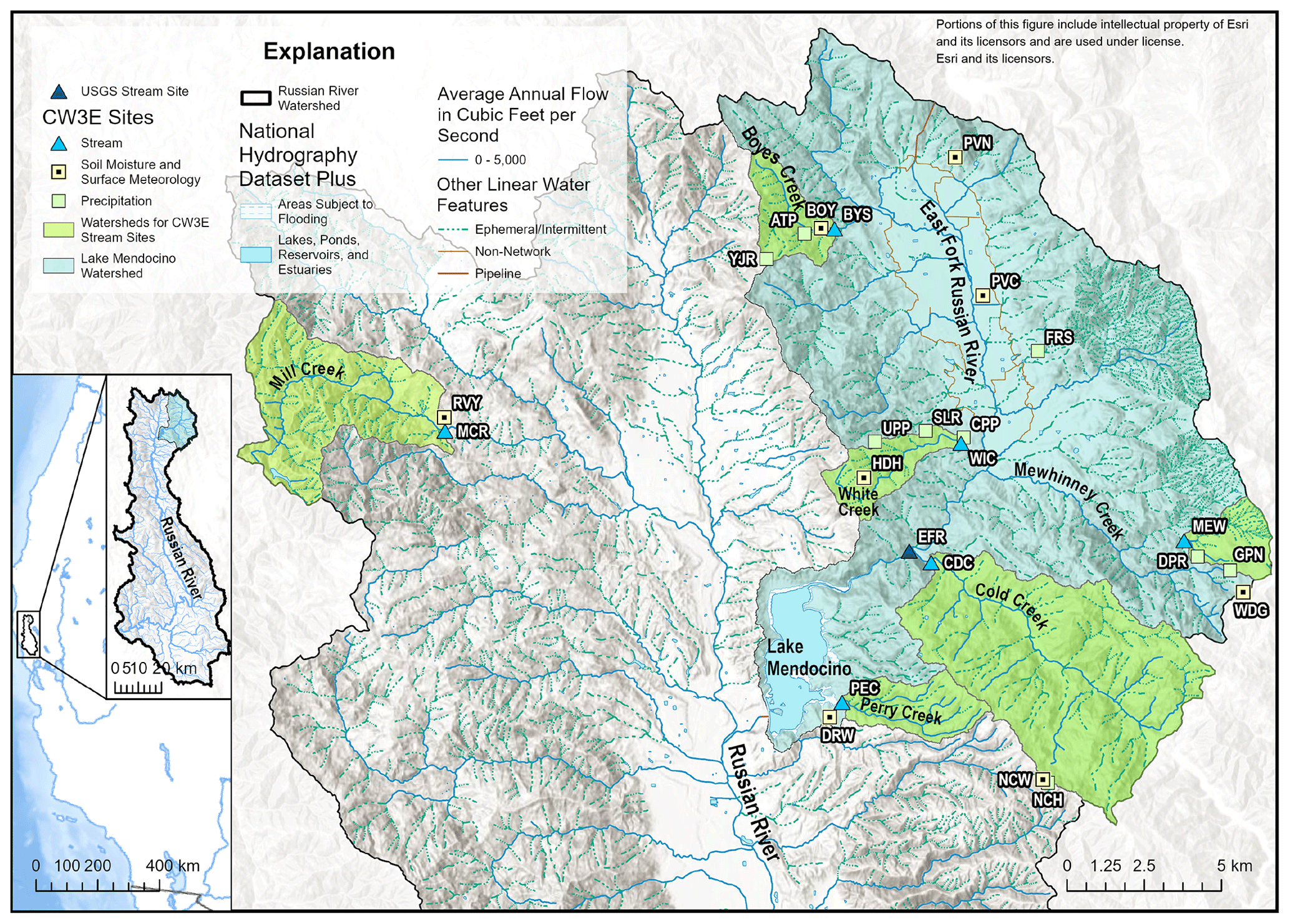
Figure A1Location of the U.S. Geological Survey streamgage 11461500 (EFR) and Center for Western Weather and Water Extremes (CW3E) stream, precipitation, and surface meteorology sites in the upper Russian River watershed, California. Image data sources: CW3E and National Hydrography Dataset Plus (NHDPlus) High Resolution (Moore et al., 2019; Esri).
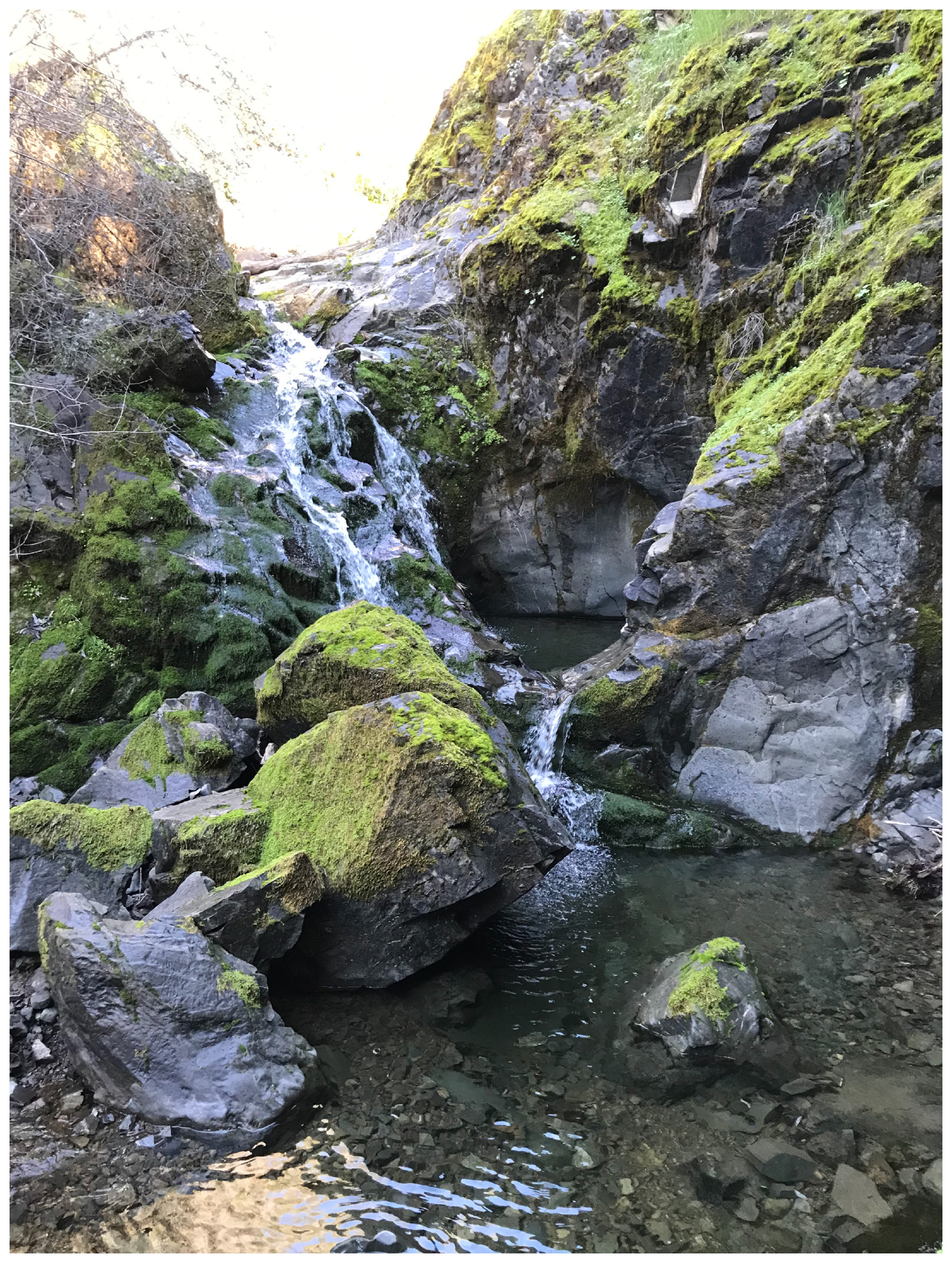
Figure A2Waterfall flowing over mossy Franciscan sandstone just upstream of the Perry Creek (PEC) stream site from January 2022.
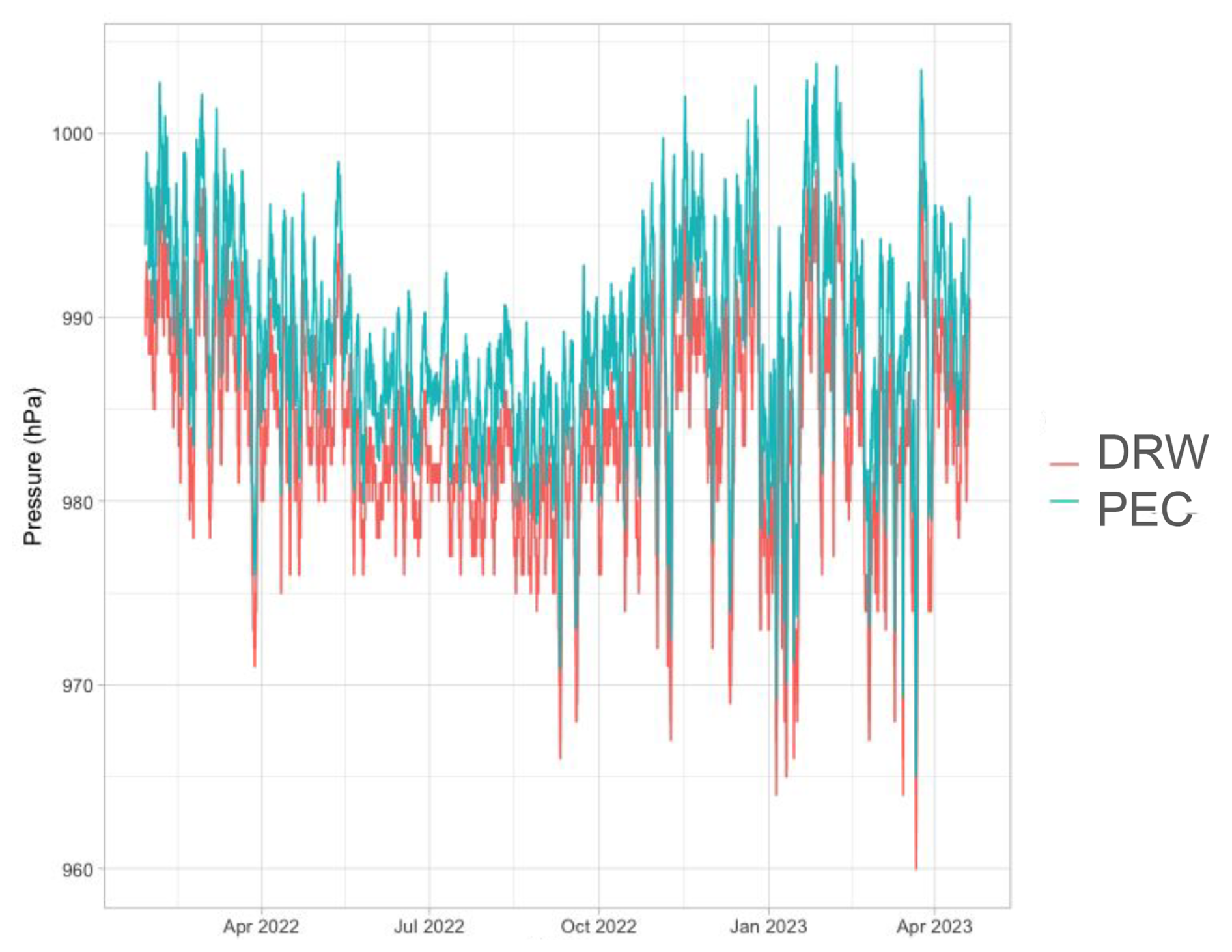
Figure A3Perry Creek (PEC) barologger atmospheric pressure and Deerwood (DRW) surface meteorology site atmospheric pressure.
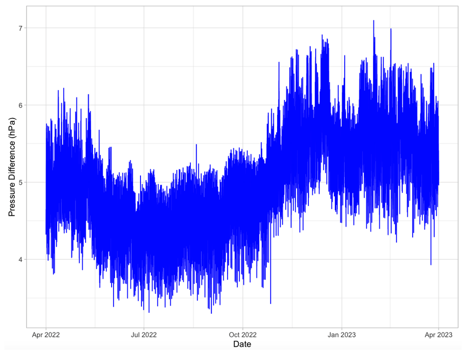
Figure A4Difference between Perry Creek (PEC) barologger atmospheric pressure and Deerwood (DRW) atmospheric pressure from April 2022 through March 2023.
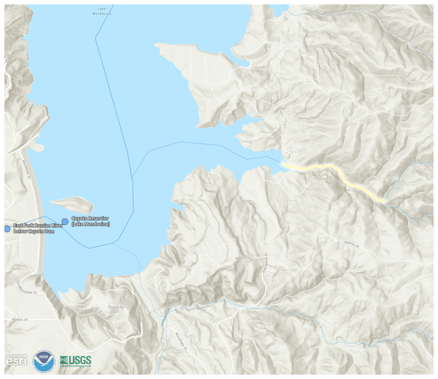
Figure A5The National Water Model segment of Perry Creek that overlaps with the Perry Creek (PEC) monitoring site. The stream segment is highlighted in light yellow, and the PEC site (not shown) is located just upstream of Lake Mendocino along the stream segment in this image. Image source: Esri, NOAA (2024b).
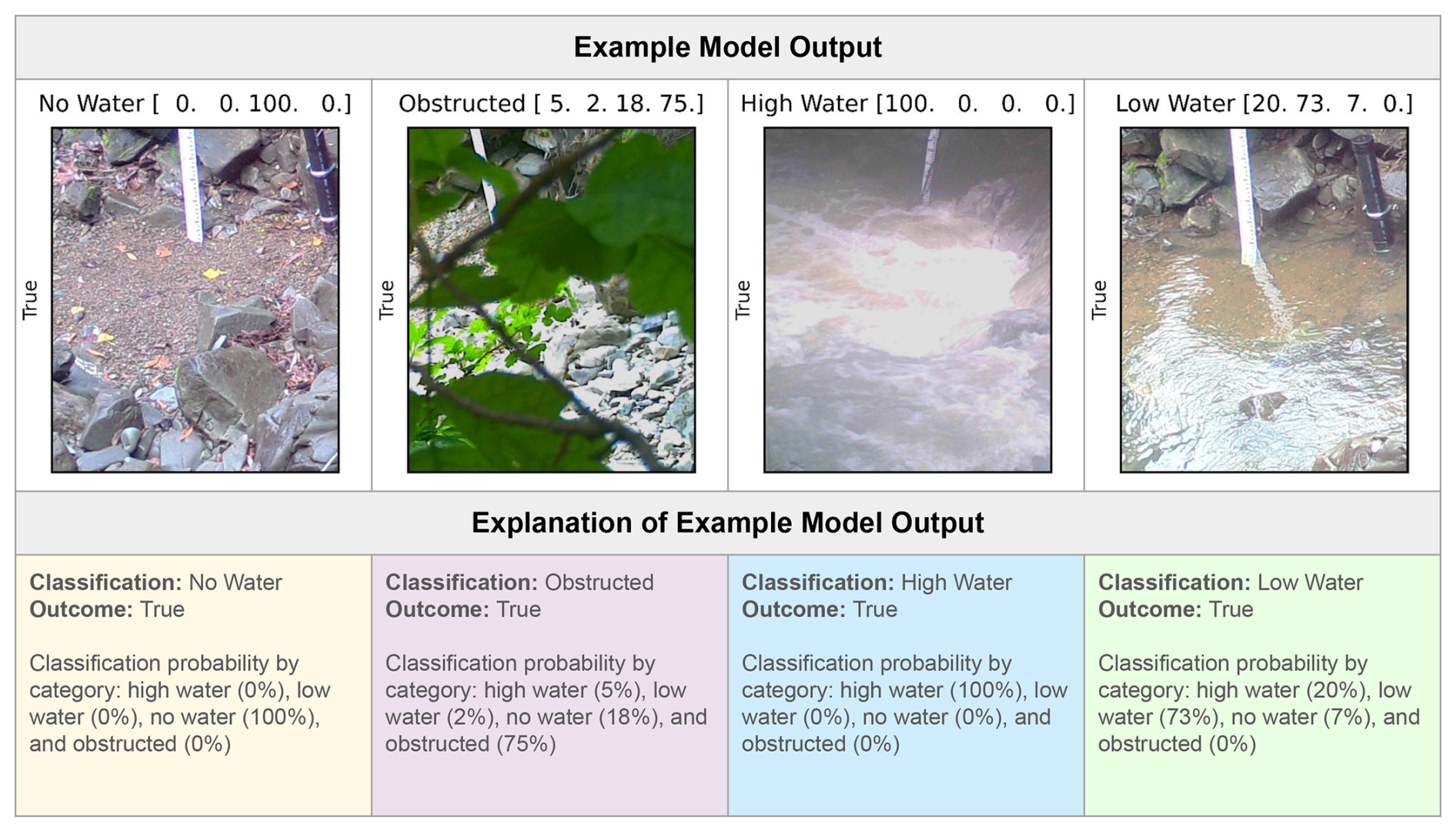
Figure A6A sample of labeled test set images and corresponding classification outputs from the final model run. The images are annotated (text above images) with the classification (high water, low water, no water, or obstructed category labels) and the classification probabilities for each category (%). The simple outcome (“True” for correct classifications and “False” for incorrect classifications) is to the left of each image. A detailed explanation of the classification output is below each corresponding image.
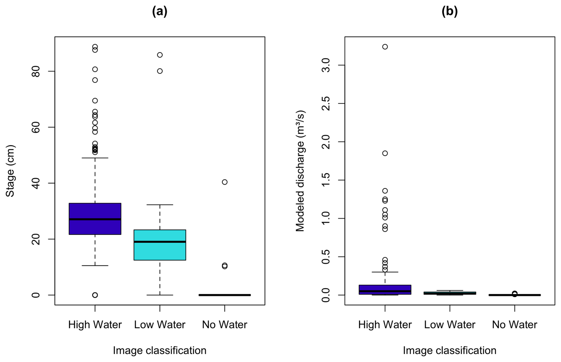
Figure A7Distribution of Perry Creek (PEC) stage and modeled discharge for medium- and high-confidence image classifications. The boxplots show all values for stage (a) and modeled discharge (b) at PEC (vertical axis) corresponding to medium- and high-confidence (only) classifications of images as high, low, and no water (horizontal axis). The boxplots show the interquartile range (IQR; box), median (bold line), the upper/lower quartile ±1.5 ⋅ IQR (whiskers), and outliers (points).
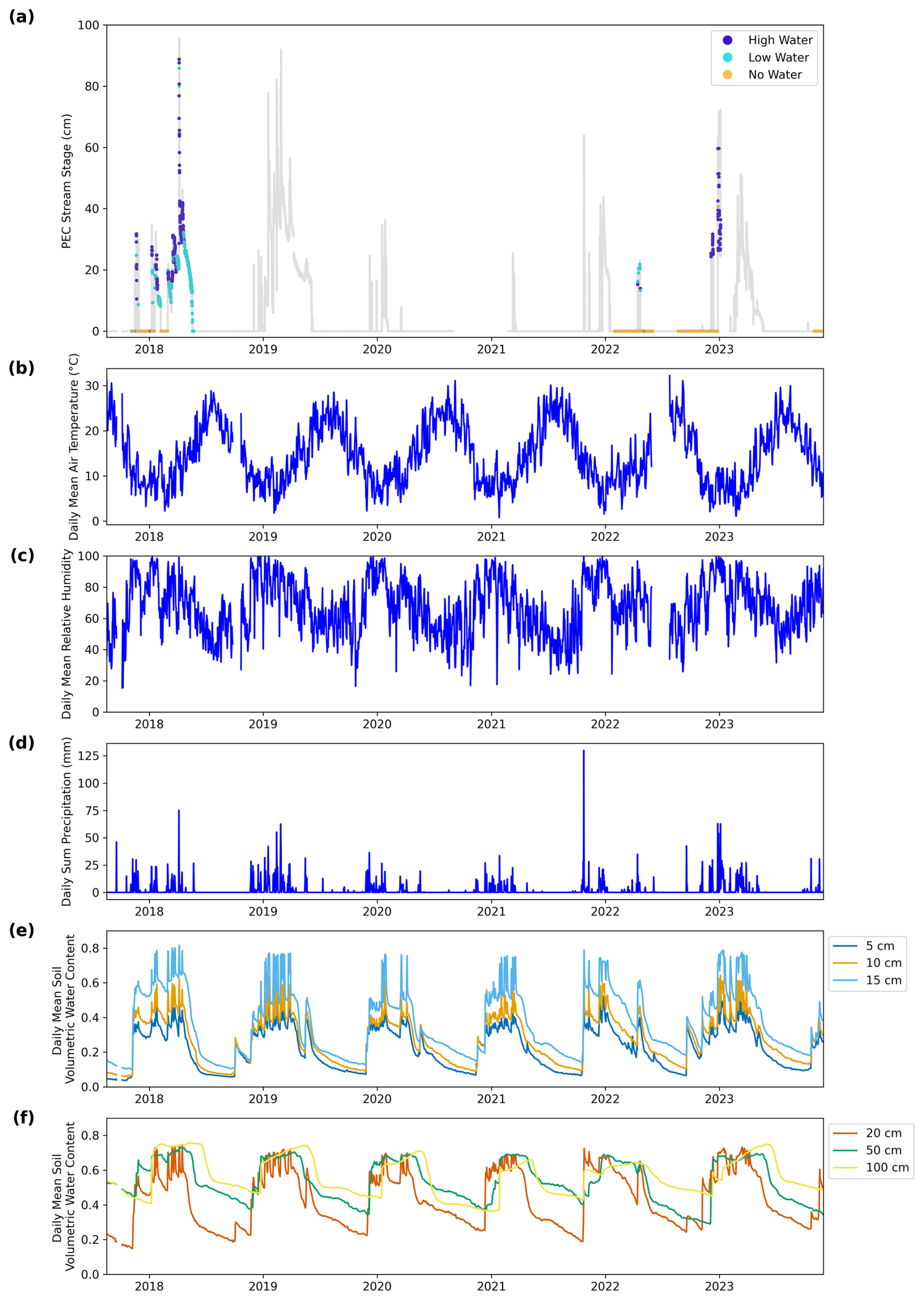
Figure A8Perry Creek (PEC) stage and Deerwood (DRW) site meteorology and soil moisture, August 2017–November 2023. Time series include: (a) 15 min barometrically compensated and quality controlled PEC stage colored by concurrent medium or high-confidence image classifications; and daily DRW (b) mean air temperature, (c) mean relative humidity, (d) total precipitation, (e) mean soil volumetric water content (at depths of 5, 10, and 15 cm), and (f) mean soil volumetric water content (at depths of 20, 50, and 100 cm).
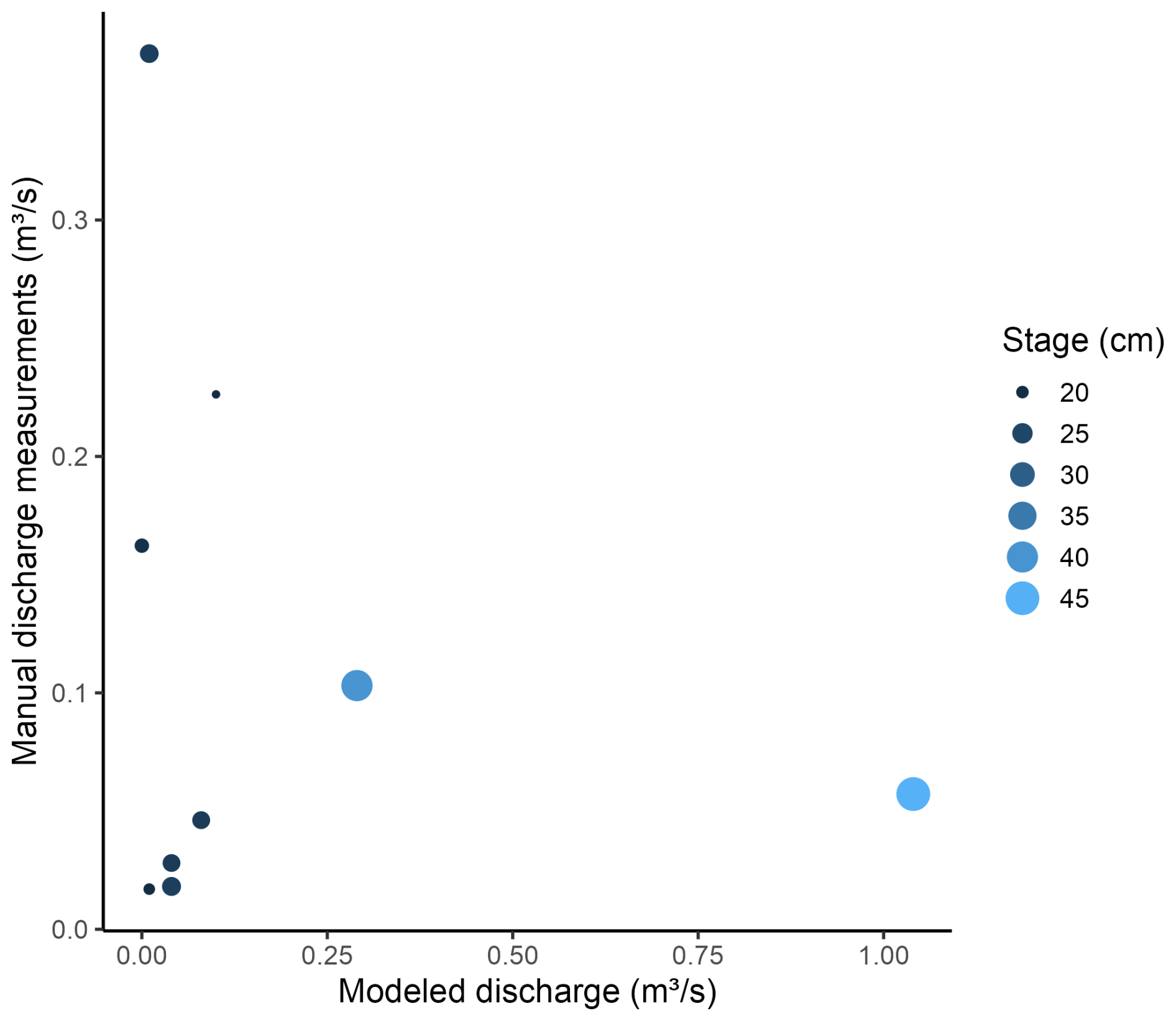
Figure A9National Water Model (NWM) discharge and manual discharge measurements at Perry Creek. Points show available concurrent observations of measured discharge (vertical axis) at the Perry Creek (PEC) site and modeled discharge (horizontal axis) at a stream segment overlapping PEC, which are colored by observed PEC stage.
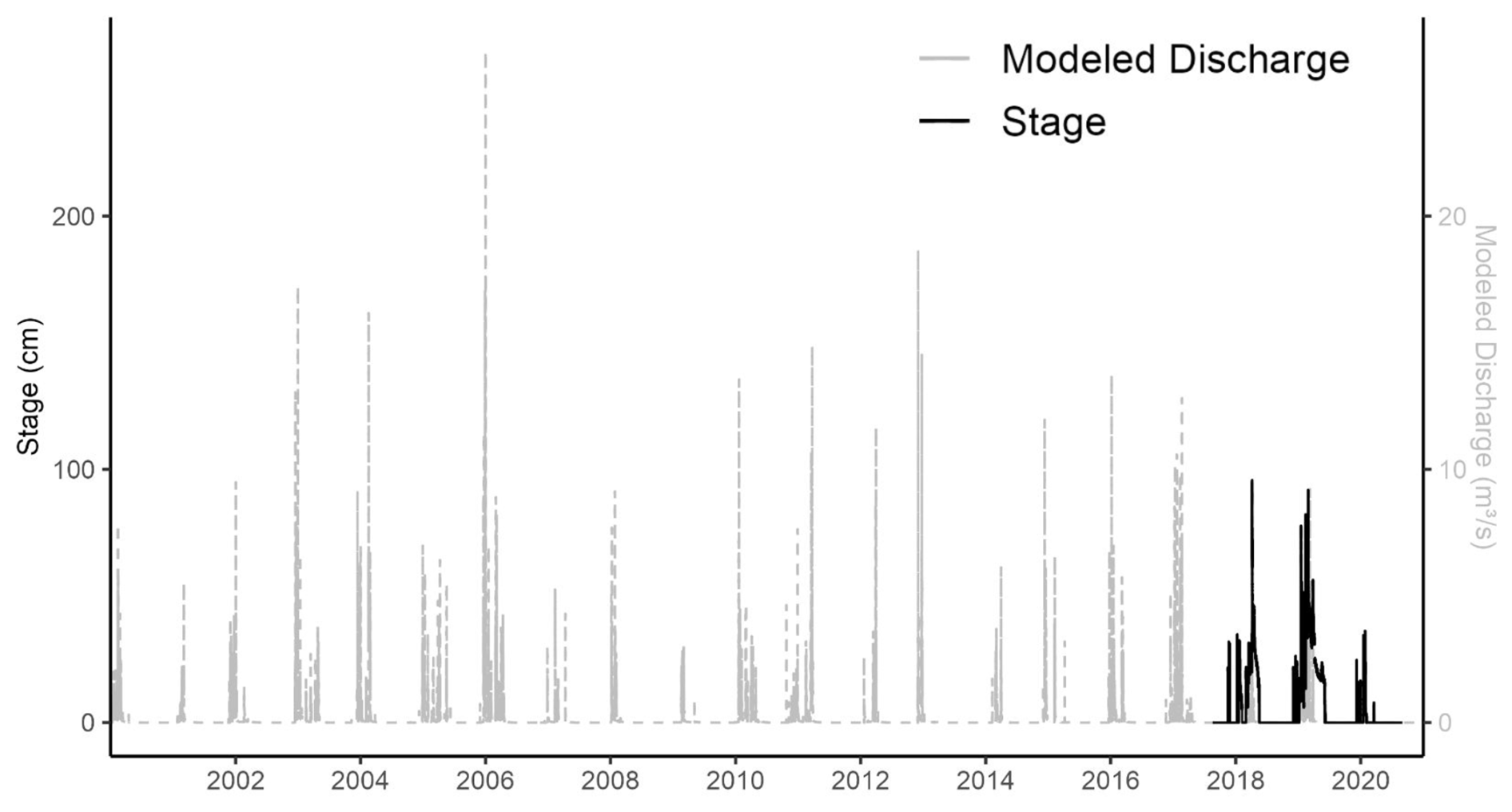
Figure A10Time series of National Water Model (NWM) discharge and stage measurements at Perry Creek. Lines show partially-overlapping observations of observed stage at the Perry Creek (PEC) site (left vertical axis, solid black line) between 2017–2020, and modeled discharge (right vertical axis, dotted gray line) at a stream segment overlapping PEC between 2000–2020.
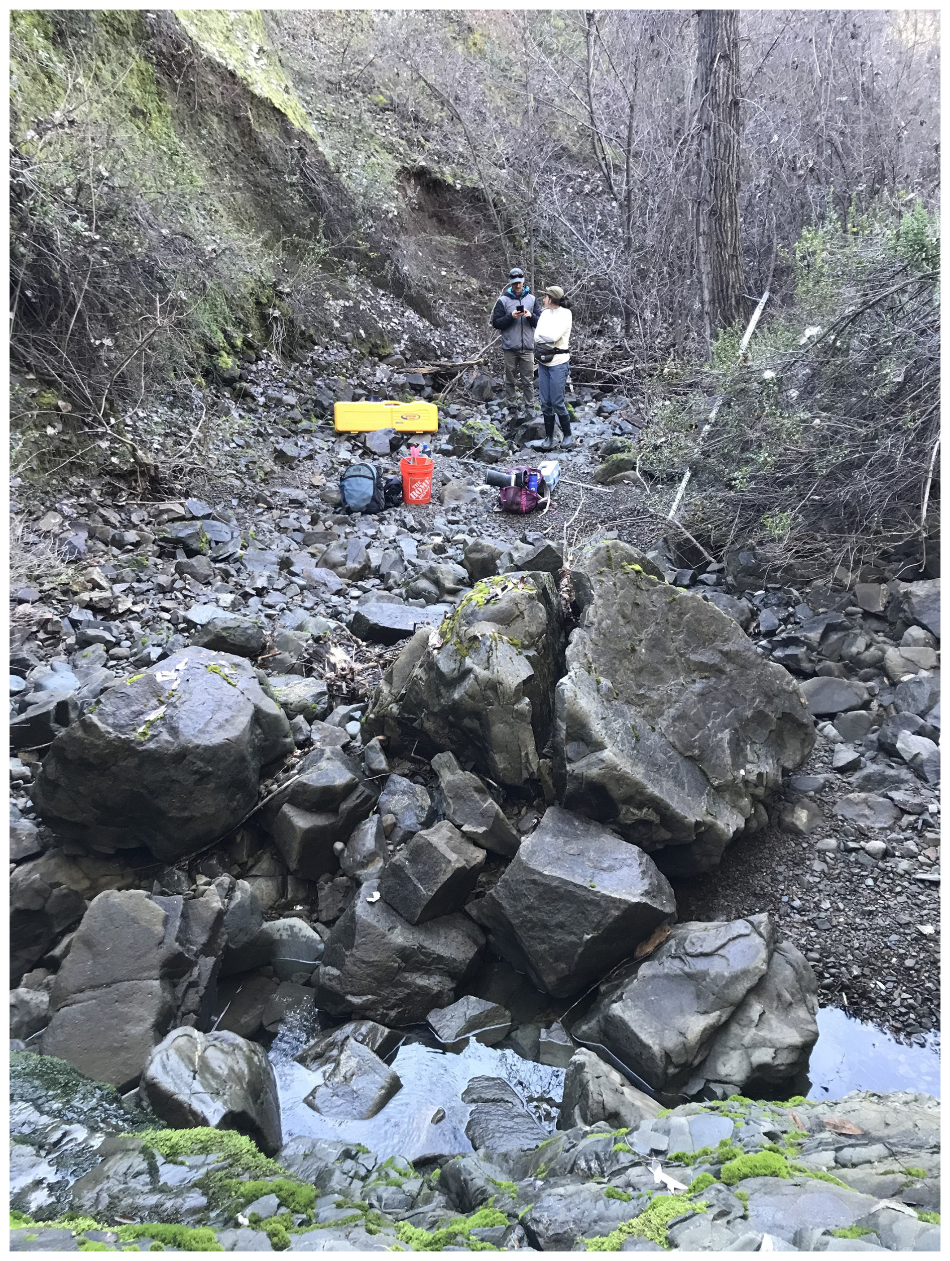
Figure A11Photo from a Perry Creek (PEC) site visit in January 2022. The photo shows a small pool of water upstream of the PEC site in front of the last visible outcrop of Franciscan sandstone. The rocky, dry streambed is visible in the middle, with the white staff plate on the right. The steep hillside on the left is a landslide deposit. This photo was taken looking downstream.
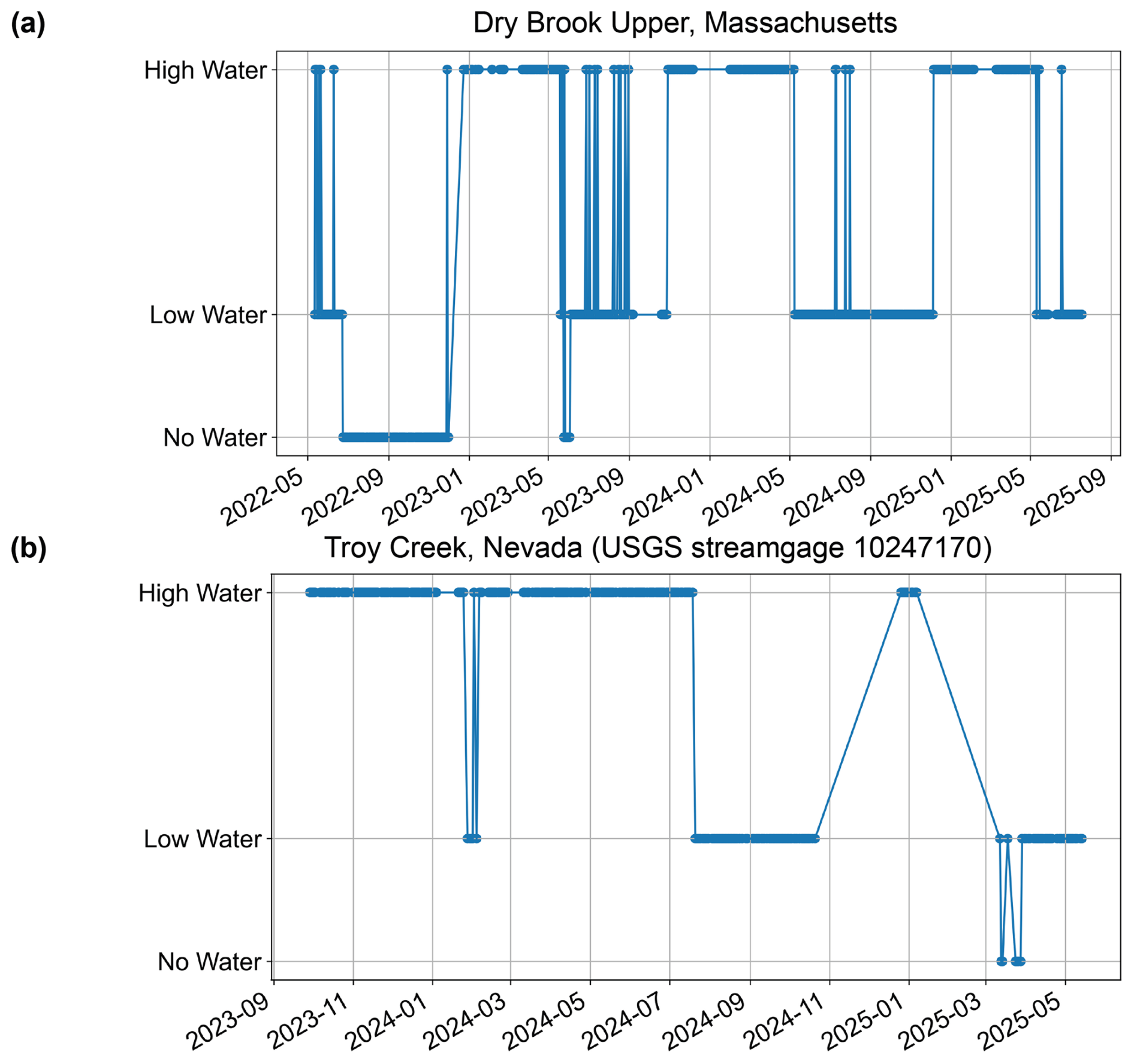
Table A1Percentages of images classified as no, low, and high water that correspond to stage or discharge greater than: percentiles of observed stage at Perry Creek (PEC) from August, 2017 through November, 2023 (top); National Water Model (NWM) discharge at a stream segment overlapping PEC from August, 2017 through August, 2020 (middle); and NWM discharge from January, 2000 through December, 2020 (bottom). All percentages were calculated using the same medium- and high-confidence image classifications from August, 2017 through November, 2023. For NWM data, only image classifications from 2017–2018 are used because there is no NWM data after 2020, and there are no images available during 2019 and 2020.
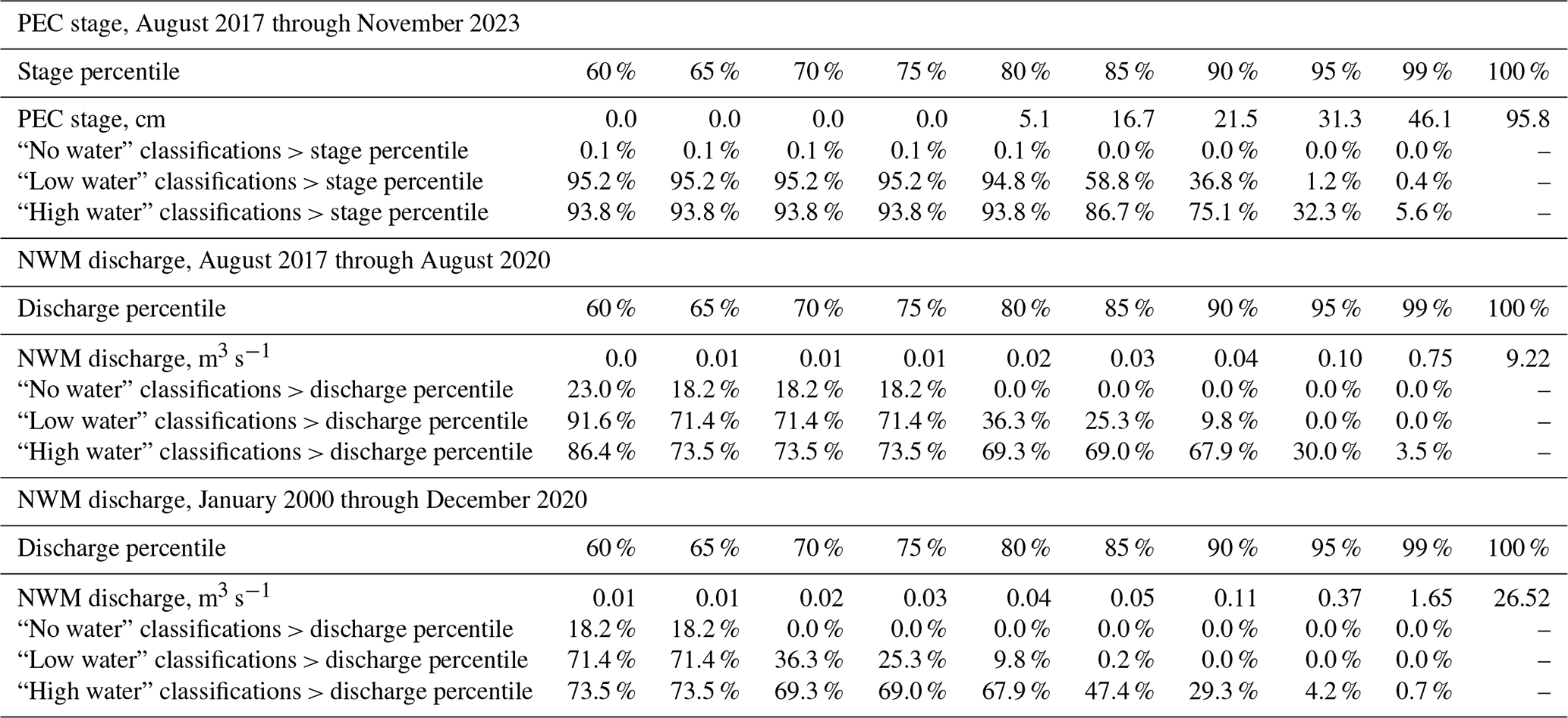
Code that implements the final model, associated data from this study (images, PEC stage data, PEC manual discharge data, DRW soil and surface meteorology data, and NWM discharge data), and instructions for applying our methodology to USGS Flow Photo Explorer images are publicly available and citable on the CUAHSI HydroShare platform at: http://www.hydroshare.org/resource/926f16b0d54242879777b19fa805ef79 (Ogle and Levy, 2025).
S.E.O. and M.C.L conceptualized the research and methodology, and M.C.L. supervised the research. S.E.O. worked with M.C.L. to perform the analysis. G.M. managed the stream sites and described them in the manuscript. S.E.O., G.M., and A.J. processed and visualized the stream data. S.E.O. and M.C.L drafted the manuscript, and S.E.O. and M.C.L. edited the manuscript with contributions from all authors. M.C.L. and F.M.R. managed funding acquisition.
The contact author has declared that none of the authors has any competing interests.
Publisher's note: Copernicus Publications remains neutral with regard to jurisdictional claims made in the text, published maps, institutional affiliations, or any other geographical representation in this paper. The authors bear the ultimate responsibility for providing appropriate place names. Views expressed in the text are those of the authors and do not necessarily reflect the views of the publisher.
S.E.O. thanks the CW3E field team, especially Sarah Burnett and Adolfo Lopez along with support from Duncan Watson-Parris, Konstantine Georgakakos, Ming Pan, Adrian Borsa, Patrick Mulrooney, Agniv Sengupta, Michael Dettinger, and Peter Yao. We also thank CW3E's Russian River cooperators: stakeholders, landowners, and FIRO partners including the U.S. Army Corps of Engineers, Sonoma County Water Agency, and the California Department of Water Resources.
This research has been supported by a Hellman Fellows Program (faculty) award, a NSF Award (grant no. 2205239), and the U.S. Army Corps of Engineers Engineer Research and Development Center FIRO program (grant no. Award USACE W912HZ-24-2-0001).
This paper was edited by Alberto Guadagnini and reviewed by two anonymous referees.
Acuña, V., Datry, T., Marshall, J., Barceló, D., Dahm, C. N., Ginebreda, A., McGregor, G., Sabater, S., Tockner, K., and Palmer, M. A.: Why Should We Care About Temporary Waterways?, Science, 343, 1080–1081, https://doi.org/10.1126/science.1246666, 2014. a, b, c, d
Albano, C. M., Abatzoglou, J. T., McEvoy, D. J., Huntington, J. L., Morton, C. G., Dettinger, M. D., and Ott, T. J.: A Multidataset Assessment of Climatic Drivers and Uncertainties of Recent Trends in Evaporative Demand across the Continental United States, Journal of Hydrometeorology, 23, 505–519, https://doi.org/10.1175/JHM-D-21-0163.1, 2022. a
AMS: Forecast-informed reservoir operations, American Meteorological Society (AMS) Glossary of Meteorology, http://glossary.ametsoc.org/wiki/Forecast-informed_reservoir_operations (last access: 27 January 2026), 2020. a
Arismendi, I., Dunham, J., Heck, M., Schultz, L., and Hockman-Wert, D.: A Statistical Method to Predict Flow Permanence in Dryland Streams from Time Series of Stream Temperature, Water, 9, 946, https://doi.org/10.3390/w9120946, 2017. a
Bertassello, L., Levy, M. C., and Müller, M. F.: Sociohydrology, ecohydrology, and the space-time dynamics of human-altered catchments, Hydrological Sciences Journal, 66, 1393–1408, https://doi.org/10.1080/02626667.2021.1948550, 2021. a
Birgand, F., Chapman, K., Hazra, A., Gilmore, T., Etheridge, R., and Staicu, A.-M.: Field performance of the GaugeCam image-based water level measurement system, PLOS Water, 1, e0000032, https://doi.org/10.1371/journal.pwat.0000032, 2022. a
Cardwell, G. T.: Geology and ground water in Russian River Valley areas and in Round, Laytonville, and Little Lake Valleys, Sonoma and Mendocino Counties, California, Tech. Rep. 1548, U.S. Govt. Print. Off., https://doi.org/10.3133/wsp1548, 1965. a
Carpenter, T. M. and Georgakakos, K. P.: Impacts of parametric and radar rainfall uncertainty on the ensemble streamflow simulations of a distributed hydrologic model, Journal of Hydrology, 298, 202–221, https://doi.org/10.1016/j.jhydrol.2004.03.036, 2004. a
Chagas, V. B. P., Chaffe, P. L. B., and Blöschl, G.: Regional Low Flow Hydrology: Model Development and Evaluation, 60, e2023WR035063, https://doi.org/10.1029/2023WR035063, 2024. a
Chapin, T. P., Todd, A. S., and Zeigler, M. P.: Robust, low-cost data loggers for stream temperature, flow intermittency, and relative conductivity monitoring, Water Resources Research, 50, 6542–6548, https://doi.org/10.1002/2013WR015158, 2014. a
Chapman, K. W., Gilmore, T. E., Chapman, C. D., Birgand, F., Mittelstet, A. R., Harner, M. J., Mehrubeoglu, M., and Stranzl Jr., J. E.: Open‐Source Software for Water‐Level Measurement in Images With a Calibration Target, Water Resources Research, 58, e2022WR033203, https://doi.org/10.1029/2022WR033203, 2022. a
Chiu, M.-C., Leigh, C., Mazor, R., Cid, N., and Resh, V.: Chapter 5.1 – Anthropogenic Threats to Intermittent Rivers and Ephemeral Streams, in: Intermittent Rivers and Ephemeral Streams, edited by Datry, T., Bonada, N., and Boulton, A., Academic Press, 433–454, ISBN 978-0-12-803835-2, https://doi.org/10.1016/B978-0-12-803835-2.00017-6, 2017. a
Cosgrove, B., Gochis, D., Flowers, T., Dugger, A., Ogden, F., Graziano, T., Clark, E., Cabell, R., Casiday, N., Cui, Z., Eicher, K., Fall, G., Feng, X., Fitzgerald, K., Frazier, N., George, C., Gibbs, R., Hernandez, L., Johnson, D., Jones, R., Karsten, L., Kefelegn, H., Kitzmiller, D., Lee, H., Liu, Y., Mashriqui, H., Mattern, D., McCluskey, A., McCreight, J. L., McDaniel, R., Midekisa, A., Newman, A., Pan, L., Pham, C., RafieeiNasab, A., Rasmussen, R., Read, L., Rezaeianzadeh, M., Salas, F., Sang, D., Sampson, K., Schneider, T., Shi, Q., Sood, G., Wood, A., Wu, W., Yates, D., Yu, W., and Zhang, Y.: NOAA's National Water Model: Advancing operational hydrology through continental-scale modeling, JAWRA Journal of the American Water Resources Association, 60, 247–272, 2024. a, b
CrowdWater: Temporary Stream – CrowdWater, https://crowdwater.ch/en/temporary-stream/ (last access: 27 January 2026), 2023. a
Dalal, N. and Triggs, B.: Histograms of oriented gradients for human detection, in: 2005 IEEE Computer Society Conference on Computer Vision and Pattern Recognition (CVPR'05), vol. 1, 886–893, https://doi.org/10.1109/CVPR.2005.177, 2005. a
Datry, T., Bonada, N., and Boulton, A. J.: General Introduction, in: Intermittent Rivers and Ephemeral Streams, Elsevier, 1–20, ISBN 978-0-12-803835-2, https://doi.org/10.1016/B978-0-12-803835-2.00001-2, 2017. a
Delattre, M. P. and Rubin, R. S.: Preliminary Geologic Map of the Ukiah 7.5’ Quadrangle, Mendocino County, California, Tech. rep., California Geological Survey, https://ngmdb.usgs.gov/Prodesc/proddesc_110798.htm (last access: 27 January 2026), 2020. a, b, c, d, e
Dettinger, M.: Historical and Future Relations Between Large Storms and Droughts in California, San Francisco Estuary and Watershed Science, 14, https://doi.org/10.15447/sfews.2016v14iss2art1, 2016. a
Dettinger, M., Wilson, A., and McGurk, G.: Keeping Water in Climate-Changed Headwaters Longer, San Francisco Estuary and Watershed Science, San Francisco Estuary & Watershed Science, 21, https://doi.org/10.15447/sfews.2023v21iss4art1, 2023. a, b
Durighetto, N. and Botter, G.: Time‐lapse visualization of spatial and temporal patterns of stream network dynamics, Hydrological Processes, 35, e14053, https://doi.org/10.1002/hyp.14053, 2021. a
Fei, J., Liu, J., Ke, L., Wang, W., Wu, P., and Zhou, Y.: A deep learning-based method for mapping alpine intermittent rivers and ephemeral streams of the Tibetan Plateau from Sentinel-1 time series and DEMs, Remote Sensing of Environment, 282, 113271, https://doi.org/10.1016/j.rse.2022.113271, 2022. a
Feng, D., Beck, H., Lawson, K., and Shen, C.: The suitability of differentiable, physics-informed machine learning hydrologic models for ungauged regions and climate change impact assessment, Hydrology and Earth System Sciences, 27, 2357–2373, https://doi.org/10.5194/hess-27-2357-2023, 2023. a
Forghanparast, F. and Mohammadi, G.: Using Deep Learning Algorithms for Intermittent Streamflow Prediction in the Headwaters of the Colorado River, Texas, Water, 14, 2972, https://doi.org/10.3390/w14192972, 2022. a
Fovet, O., Belemtougri, A., Boithias, L., Braud, I., Charlier, J.-B., Cottet, M., Daudin, K., Dramais, G., Ducharne, A., Folton, N., Grippa, M., Hector, B., Kuppel, S., Le Coz, J., Legal, L., Martin, P., Moatar, F., Molénat, J., Probst, A., Riotte, J., Vidal, J.-P., Vinatier, F., and Datry, T.: Intermittent rivers and ephemeral streams: Perspectives for critical zone science and research on socio-ecosystems, WIREs Water, 8, e1523, https://doi.org/10.1002/wat2.1523, 2021. a, b
Gershunov, A., Shulgina, T., Clemesha, R. E. S., Guirguis, K., Pierce, D. W., Dettinger, M. D., Lavers, D. A., Cayan, D. R., Polade, S. D., Kalansky, J., and Ralph, F. M.: Precipitation regime change in Western North America: The role of Atmospheric Rivers, Scientific Reports, 9, 9944, https://doi.org/10.1038/s41598-019-46169-w, 2019. a
Goodling, P. J., Fair, J. H., Gupta, A., Walker, J. D., Dubreuil, T., Hayden, M., and Letcher, B. H.: Technical note: A low-cost approach to monitoring relative streamflow dynamics in small headwater streams using time lapse imagery and a deep learning model, Hydrol. Earth Syst. Sci., 29, 6445–6460, https://doi.org/10.5194/hess-29-6445-2025, 2025. a, b, c, d
Gupta, A., Chang, T., Walker, J., and Letcher, B.: Towards Continuous Streamflow Monitoring with Time-Lapse Cameras and Deep Learning, in: ACM SIGCAS/SIGCHI Conference on Computing and Sustainable Societies (COMPASS), ACM, Seattle WA USA, 353–363, ISBN 978-1-4503-9347-8, https://doi.org/10.1145/3530190.3534805, 2022. a, b, c, d, e, f, g
Gutiérrez-Jurado, K. Y., Partington, D., Batelaan, O., Cook, P., and Shanafield, M.: What Triggers Streamflow for Intermittent Rivers and Ephemeral Streams in Low-Gradient Catchments in Mediterranean Climates, Water Resources Research, 55, 9926–9946, https://doi.org/10.1029/2019WR025041, 2019. a, b, c, d
Han, H. and Morrison, R. R.: Improved runoff forecasting performance through error predictions using a deep-learning approach, Journal of Hydrology, 608, 127653, https://doi.org/10.1016/j.jhydrol.2022.127653, 2022. a
Hayhoe, K., Cayan, D., Field, C. B., Frumhoff, P. C., Maurer, E. P., Miller, N. L., Moser, S. C., Schneider, S. H., Cahill, K. N., Cleland, E. E., Dale, L., Drapek, R., Hanemann, R. M., Kalkstein, L. S., Lenihan, J., Lunch, C. K., Neilson, R. P., Sheridan, S. C., and Verville, J. H.: Emissions pathways, climate change, and impacts on California, Proceedings of the National Academy of Sciences, 101, 12422–12427, https://doi.org/10.1073/pnas.0404500101, 2004. a
Hutley, N. R., Beecroft, R., Wagenaar, D., Soutar, J., Edwards, B., Deering, N., Grinham, A., and Albert, S.: Adaptively monitoring streamflow using a stereo computer vision system, Hydrol. Earth Syst. Sci., 27, 2051–2073, https://doi.org/10.5194/hess-27-2051-2023, 2023. a
Jasperse, J., Ralph, F. M., Anderson, M., Brekke, L., Malasavage, N., Dettinger, M. D., Forbis, J., Fuller, J., Talbot, C., Webb, R., and Haynes, A.: Lake Mendocino Forecast Informed Reservoir Operations Final Viability Assessment, Tech. rep., UC San Diego, https://escholarship.org/uc/item/3b63q04n (last access: 27 January 2026), 2020. a, b
Kaplan, N. H., Sohrt, E., Blume, T., and Weiler, M.: Monitoring ephemeral, intermittent and perennial streamflow: a dataset from 182 sites in the Attert catchment, Luxembourg, Earth Syst. Sci. Data, 11, 1363–1374, https://doi.org/10.5194/essd-11-1363-2019, 2019. a
Kerezsy, A., Gido, K., Magalhães, M. F., and Skelton, P. H.: Chapter 4.5 – The Biota of Intermittent Rivers and Ephemeral Streams: Fishes, in: Intermittent Rivers and Ephemeral Streams, edited by Datry, T., Bonada, N., and Boulton, A., Academic Press, 273–298, ISBN 978-0-12-803835-2, https://doi.org/10.1016/B978-0-12-803835-2.00010-3, 2017. a, b
Kratzert, F., Klotz, D., Herrnegger, M., Sampson, A. K., Hochreiter, S., and Nearing, G. S.: Toward Improved Predictions in Ungauged Basins: Exploiting the Power of Machine Learning, Water Resources Research, 55, 11344–11354, https://doi.org/10.1029/2019WR026065, 2019. a
Le, X.-H., Nguyen, D.-H., Jung, S., Yeon, M., and Lee, G.: Comparison of Deep Learning Techniques for River Streamflow Forecasting, IEEE Access, 9, 71805–71820, https://doi.org/10.1109/ACCESS.2021.3077703, 2021. a
Leduc, P., Ashmore, P., and Sjogren, D.: Technical note: Stage and water width measurement of a mountain stream using a simple time-lapse camera, Hydrol. Earth Syst. Sci., 22, 1–11, https://doi.org/10.5194/hess-22-1-2018, 2018. a, b, c, d
Leung, L. R., Qian, Y., Bian, X., Washington, W. M., Han, J., and Roads, J. O.: Mid-Century Ensemble Regional Climate Change Scenarios for the Western United States, Climatic Change, 62, 75–113, https://doi.org/10.1023/B:CLIM.0000013692.50640.55, 2004. a
Li, F., Zhu, Q., Riley, W. J., Yuan, K., Wu, H., and Gui, Z.: Wetter California Projected by CMIP6 Models With Observational Constraints Under a High GHG Emission Scenario, Earth's Future, 10, e2022EF002694, https://doi.org/10.1029/2022EF002694, 2022. a
Lowe, D. G.: Distinctive Image Features from Scale-Invariant Keypoints, International Journal of Computer Vision, 60, 91–110, https://doi.org/10.1023/B:VISI.0000029664.99615.94, 2004. a
Magand, C., Alves, M. H., Calleja, E., Datry, T., Dörflinger, G., England, J., Gallart, F., Gomez, R., Jorda-Capdevila, D., Marti, E., Munne, A., Pastor, A. V., Stubbington, R., Tziortzis, I., and Von Schiller, D.: Intermittent rivers and ephemeral streams: what water managers need to know, Zenodo, https://doi.org/10.5281/ZENODO.3888474, 2020. a, b
Mallakpour, I., AghaKouchak, A., and Sadegh, M.: Climate‐Induced Changes in the Risk of Hydrological Failure of Major Dams in California, Geophysical Research Letters, 46, 2130–2139, https://doi.org/10.1029/2018GL081888, 2019. a, b
McMaster-Carr: Liquid-Tight Flexible Plastic Conduit: Abrasion-Resistant, 1/2 Trade Size, https://www.mcmaster.com/7581K42/ (last access: 30 May 2024), 2024. a
Moidu, H., Obedzinski, M., Carlson, S. M., and Grantham, T. E.: Spatial Patterns and Sensitivity of Intermittent Stream Drying to Climate Variability, Water Resources Research, 57, e2021WR030314, https://doi.org/10.1029/2021WR030314, 2021. a
Moore, R. B., McKay, L. D., Rea, A. H., Bondelid, T. R., Price, C. V., Dewald, T. G., and Johnston, C. M.: User's guide for the national hydrography dataset plus (NHDPlus) high resolution, Tech. Rep. 2019-1096, U.S. Geological Survey, https://doi.org/10.3133/ofr20191096, 2019. a, b, c
NOAA: NOAA National Water Model CONUS Retrospective Dataset, NOAA [data set], https://registry.opendata.aws/nwm-archive (last access: 1 April 2024), 2024a. a, b
NOAA: National Water Model Map, https://water.noaa.gov/map (last access: 13 November 2024), 2024b. a
Noto, S., Tauro, F., Petroselli, A., Apollonio, C., Botter, G., and Grimaldi, S.: Low-cost stage-camera system for continuous water-level monitoring in ephemeral streams, Hydrological Sciences Journal, 67, 1439–1448, https://doi.org/10.1080/02626667.2022.2079415, 2022. a, b, c, d
Ogle, S. E. and Levy, M. C.: Code and data for “Image-based classification of stream stage to support ephemeral stream monitoring”, HydroShare [data set] and [code], http://www.hydroshare.org/resource/926f16b0d54242879777b19fa805ef79, 2025. a
Osborne, W. A.: Listening to Rivers: Using sound to monitor rivers, PhD thesis, Durham University, http://etheses.dur.ac.uk/14377/ (last access: 27 January 2026), 2022. a
Otsu, N.: A Threshold Selection Method from Gray-Level Histograms, IEEE Transactions on Systems, Man, and Cybernetics, 9, 62–66, https://ieeexplore.ieee.org/document/4310076 (last access: 3 February 2026), 1979. a, b
Pedregosa, F., Varoquaux, G., Gramfort, A., Michel, V., Thirion, B., Grisel, O., Blondel, M., Prettenhofer, P., Weiss, R., Dubourg, V., Vanderplas, J., Passos, A., Cournapeau, D., Brucher, M., Perrot, M., and Duchesnay, E.: Scikit-Learn: Machine Learning in Python, https://scikit-learn.org/stable/modules/linear_model.html#multinomial-case (last access: 17 March 2025), 2011a. a
Pedregosa, F.., Varoquaux, G., Gramfort, A., Michel, V., Thirion, B., Grisel, O., Blondel, M., Prettenhofer, P., Weiss, R., Dubourg, V.., Vanderplas, J., Passos, A., Cournapeau, D., Brucher, M., Perrot, M., and Duchesnay, E.: LogisticRegressionCV, https://scikit-learn.org/stable/modules/generated/sklearn.linear_model.LogisticRegressionCV.html#sklearn.linear_model.LogisticRegressionCV (last access: 17 March 2025), 2011b. a
Pedregosa, F., Varoquaux, G., Gramfort, A., Michel, V., Thirion, B., Grisel, Pedregosa, F.., Varoquaux, G., Gramfort, A., Michel, V., Thirion, B., Grisel, O., Blondel, M., Prettenhofer, P., Weiss, R., Dubourg, V.., Vanderplas, J., Passos, A., Cournapeau, D., Brucher, M., Perrot, M., and Duchesnay, E.: Scikit-Learn: Machine Learning in Python, Machine Learning in Python, https://dl.acm.org/doi/10.5555/1953048.2078195 (last access: 27 January 2026), 2011c. a, b, c, d
Persad, G. G., Swain, D. L., Kouba, C., and Ortiz-Partida, J. P.: Inter-model agreement on projected shifts in California hydroclimate characteristics critical to water management, Climatic Change, 162, 1493–1513, https://doi.org/10.1007/s10584-020-02882-4, 2020. a
Pierce, D. W., Cayan, D. R., Das, T., Maurer, E. P., Miller, N. L., Bao, Y., Kanamitsu, M., Yoshimura, K., Snyder, M. A., Sloan, L. C., Franco, G., and Tyree, M.: The Key Role of Heavy Precipitation Events in Climate Model Disagreements of Future Annual Precipitation Changes in California, Journal of Climate, 26, 5879–5896, https://doi.org/10.1175/JCLI-D-12-00766.1, 2013. a
Polade, S. D., Pierce, D. W., Cayan, D. R., Gershunov, A., and Dettinger, M. D.: The key role of dry days in changing regional climate and precipitation regimes, Scientific Reports, 4, 4364, https://doi.org/10.1038/srep04364, 2014. a
Polade, S. D., Gershunov, A., Cayan, D. R., Dettinger, M. D., and Pierce, D. W.: Precipitation in a warming world: Assessing projected hydro-climate changes in California and other Mediterranean climate regions, Scientific Reports, 7, 10783, https://doi.org/10.1038/s41598-017-11285-y, 2017. a
Ralph, F. M., Wilson, A. M., Alden, D., Ellis, C. J., Cooper, A., Paulsson, K., Kawzenuk, B. K., and Yao, P.: Center for Western Weather and Water Extremes (CW3E) Surface Meteorological Observational Dataset, UC San Diego Library Digital Collections [data set], https://doi.org/10.6075/J0SX6DDH, 2022. a
Rodrigues, R. M., Braga, B. B., and Costa, C. A. G.: Efficiency in river discharge measurement: combining Chiu’s method with particle image velocimetry techniques, Revista Brasileira de Recursos Hídricos (RBRH), 30, e31, https://doi.org/10.1590/2318-0331.302520240125, 2025. a
Scott River Watershed Council: Scott River Coho Salmon Spawning Ground Survey, 2024–2025 Season, Tech. rep., Scott River Watershed Council, https://scottriver.org/wp-content/uploads/2025/03/Scott-River-Coho-Salmon-Spawning-Ground-Survey-2024-2025-Season.pdf (last access: 2 February 2026), 2025. a
Seibert, J., Strobl, B., Etter, S., Hummer, P., and van Meerveld, H. J. I.: Virtual Staff Gauges for Crowd-Based Stream Level Observations, Frontiers in Earth Science, 7, https://www.frontiersin.org/articles/10.3389/feart.2019.00070 (last access: 2 February 2026), 2019. a, b
Shulgina, T., Gershunov, A., Hatchett, B. J., Guirguis, K., Subramanian, A. C., Margulis, S. A., Fang, Y., Cayan, D. R., Pierce, D. W., Dettinger, M., Anderson, M. L., and Ralph, F. M.: Observed and projected changes in snow accumulation and snowline in California's snowy mountains, Climate Dynamics, https://doi.org/10.1007/s00382-023-06776-w, 2023. a
Soil Survey Staff at the Natural Resources Conservation Service at the US Department of Agriculture: Web Soil Survey, https://websoilsurvey.nrcs.usda.gov/ (last access: 20 August 2024), 2024. a, b, c
SPOTTERON GmbH: CrowdWater, https://apps.apple.com/us/app/crowdwater-spotteron/id1213513623 (last access: 2 February 2026), 2025. a
Stubbington, R., Bogan, M. T., Bonada, N., Boulton, A. J., Datry, T., Leigh, C., and Vander Vorste, R.: Chapter 4.3 – The Biota of Intermittent Rivers and Ephemeral Streams: Aquatic Invertebrates, in: Intermittent Rivers and Ephemeral Streams, edited by Datry, T., Bonada, N., and Boulton, A., Academic Press, 217–243, ISBN 978-0-12-803835-2, https://doi.org/10.1016/B978-0-12-803835-2.00007-3, 2017. a
Sumargo, E., McMillan, H., Weihs, R., Ellis, C. J., Wilson, A. M., and Ralph, F. M.: A soil moisture monitoring network to assess controls on runoff generation during atmospheric river events, Hydrological Processes, 35, e13998, https://doi.org/10.1002/hyp.13998, 2021. a, b
Takagi, Y., Tsujikawa, A., Takato, M., Saito, T., and Kaida, M.: Development of a noncontact liquid level measuring system using image processing, Water Science and Technology, 37, 381–387, https://doi.org/10.2166/wst.1998.0564, 1998. a
Tosi, F., Rocca, M., Aleotti, F., Poggi, M., Mattoccia, S., Tauro, F., Toth, E., and Grimaldi, S.: Enabling Image-Based Streamflow Monitoring at the Edge, Remote Sensing, 12, 2047, https://doi.org/10.3390/rs12122047, 2020. a
Truchy, A., Csabai, Z., Mimeau, L., Künne, A., Pernecker, B., Bertin, W., Pellizzaro, F., and Datry, T.: Citizen scientists can help advance the science and management of intermittent rivers and ephemeral streams, BioScience, 73, 513–521, https://doi.org/10.1093/biosci/biad045, 2023. a
Tulbure, M. G., Broich, M., Perin, V., Gaines, M., Ju, J., Stehman, S. V., Pavelsky, T., Masek, J. G., Yin, S., Mai, J., and Betbeder-Matibet, L.: Can we detect more ephemeral floods with higher density harmonized Landsat Sentinel 2 data compared to Landsat 8 alone?, ISPRS Journal of Photogrammetry and Remote Sensing, 185, 232–246, https://doi.org/10.1016/j.isprsjprs.2022.01.021, 2022. a
Turnipseed, D. P. and Sauer, V. B.: Discharge Measurements at Gaging Stations, in: U.S. Geological Survey Techniques and Methods, chap. A8, p. 87, U.S. Geological Survey, https://pubs.usgs.gov/tm/tm3-a8/tm3a8.pdf (last access: 2 February 2026), 2010. a
Underwood, E. C., Hollander, A. D., Flint, L. E., Flint, A. L., and Safford, H. D.: Climate change impacts on hydrological services in southern California, Environmental Research Letters, 13, 124019, https://doi.org/10.1088/1748-9326/aaeb59, 2018. a
USGS: National Land Cover Dataset (NLCD) 2021 Land Cover California Subset, https://www.arcgis.com/home/item.html?id=8e336f9a4a644db3b8627f07a7e19d97 (last access: 1 April 2024), 2023. a, b
USGS: Flow Water Explorer, https://www.usgs.gov/apps/ecosheds/fpe/#/ (last access: 2 February 2026), 2024. a, b, c, d, e, f
Van der Walt, S., Schönberger, J. L., Nunez-Iglesias, J., Boulogne, F., Warner, J. D., Yager, N., Gouillart, E., Yu, T., and the scikit-image contributors: scikit-image: Image processing in Python, PeerJ, 2, e453, https://doi.org/10.7717/peerj.453, 2014. a
Vicuna, S. and Dracup, J. A.: The evolution of climate change impact studies on hydrology and water resources in California, Climatic Change, 82, 327–350, https://doi.org/10.1007/s10584-006-9207-2, 2007. a
Vlah, M. J., Ross, M. R. V., Rhea, S., and Bernhardt, E. S.: Leveraging gauge networks and strategic discharge measurements to aid the development of continuous streamflow records, Hydrol. Earth Syst. Sci., 28, 545–573, https://doi.org/10.5194/hess-28-545-2024, 2024. a, b, c
Windheuser, L., Karanjit, R., Pally, R., Samadi, S., and Hubig, N. C.: An End-To-End Flood Stage Prediction System Using Deep Neural Networks, Earth and Space Science, 10, e2022EA002385, https://doi.org/10.1029/2022EA002385, 2023. a
Zhang, Zhou, Liu, Zhang, and Wang: Visual Measurement of Water Level under Complex Illumination Conditions, Sensors, 19, 4141, https://doi.org/10.3390/s19194141, 2019. a, b, c