
the Creative Commons Attribution 4.0 License.
the Creative Commons Attribution 4.0 License.
 | 16 Nov 2026
Covariance-informed spatiotemporal clustering improves the detection of hazardous weather events
Hunter C. Quintal

Marc L. Serre
Wiebke S. Jäger
Marleen C. de Ruiter
Spatiotemporal clustering can be used to detect weather events in multi-dimensional datasets. This method requires that the resolution of a dataset equivalently resolves variability across space and time, thereby normalizing the dataset for unbiased clustering across three dimensions. While spatiotemporal clustering is widely used, few studies quantitatively assess whether a dataset's resolution satisfies the normalization assumption required for unbiased clustering. To address this methodological gap, we present a framework to quantify the relationship between space and time using space time separable covariance modelling. We demonstrate that by defining a temporal resolution of interest (e.g., hours, days), the equivalent spatial resolution can be empirically derived using a space time metric. We present a case study using the unsupervised machine learning method Density-Based Spatial Clustering of Applications with Noise (DBSCAN) to detect extreme heat and precipitation events across the Southeastern United States between 1940 and 2023 from ECMWF Reanalysis version 5 (ERA5) data. We analyse the behaviour of space time metrics for precipitation and heat index before selecting representative values. Our results indicate that both ERA5-derived heat index and precipitation are not sufficiently resolved at their native resolutions (i.e., 0.25 spatial degrees). We demonstrate that subsequently resampling the data by the space time metric often leads to small but significant increases in the F1 score for both extreme heat and precipitation events when compared against weather warnings reported to the Iowa Environmental Mesonet from 2002 to 2023. However, even after resampling, the model exhibits poor performance, suggesting that extreme weather events with relatively small footprints cannot be resolved in reanalysis data. Despite these findings, temporal geostatistics enable measurement of the daily variability in event structure across space and time, providing novel insights into the large-scale meteorological processes (e.g., weather regimes, climate patterns) influencing observed variability.
- Article
(3157 KB) - Full-text XML
-
Supplement
(5829 KB) - BibTeX
- EndNote


Understanding trends in extreme weather events is crucial to preparedness and adaptation (Ward et al., 2020). Incomplete historical reporting of weather events has prevented comprehensive understanding of their intensity, duration, extent, and frequency (Paprotny et al., 2018, 2024). Advances in event detection within observational, reanalysis, and remotely sensed datasets has grown in recent years, leading to novel insights into event characteristics. However, differences in spatiotemporal coverage, resolution, data quality, measurement, and detection methods have resulted in inconsistent event definitions. This has been shown to impact hazard modelling results, leading to unreliable risk assessments and undermining risk management (Agulles et al., 2024). Weather events are now identified using globally resolved reanalysis data to reduce the limitations discussed above and improve consistency in event descriptions. At the regional to global scale, the application of spatiotemporal clustering to European Centre for Medium-Range Weather Forecasts (ECMWF) Reanalysis v5 (ERA5) meteorological data is now widely practiced for tracking time-evolving weather events including storms, drought, and heat waves (Rogers et al., 2022; Tilloy et al., 2022; Wibisono et al., 2021).
Spatiotemporal clustering is an unsupervised machine learning method regularly applied to weather event detection that groups extreme observations by their proximity in space and time (Ansari et al., 2020). This method assumes that spatial and temporal distances be equal prior to clustering, enabling the search for neighbouring extreme observations to be equally plausible across space and time and thus preventing preferential clustering in either dimension (Birant and Kut, 2007). To meet the normalization definition, the dataset is defined over a grid made of elemental space time cubes whereby the variation along the spatial dimension of the cube is equivalent to the variation along its temporal dimension (Bach et al., 2017). However, researchers often assume that the native resolution of a dataset satisfies this normalization definition without formal testing. This decision is problematic when the native spatial and temporal dimensions of the data do not match that of the physical processes producing weather events, leading to missed event detection (e.g., convective storms may only appear in datasets whose resolution resolves convective processes).
Geostatistical space/time covariance modelling (Kolovos et al., 2004) provides a natural framework within which to study the spatial and temporal distance scales of the variability of the physical processes that control them. It also enables researchers to test the requirement that space time cubes are properly scaled prior to clustering, yet it has not been widely applied to weather data. We hypothesize that the inclusion of covariance modelling into the spatiotemporal clustering framework would enable testing of differences between spatial and temporal resolutions, alter the weather events identified with clustering, and improve the identification of weather events in the historical record. In this paper, we introduce a method for quantifying a “space time metric” that can be used to establish whether the space time resolution of a dataset corresponds to a “space time cube” (Kisilevieh et al., 2010). The space time metric quantifies variability in space relative to time at the resolution of a given dataset. We interpret this variability to represent the structure (extent and duration) of weather fluctuations, which may quantify the scale of weather in space and time. To establish the utility of the proposed covariance-informed spatiotemporal clustering method, we apply our approach to ERA5-derived heat index and precipitation estimates to identify extreme heat and precipitation events. We find that clustering at the native resolution leads to the identification of weather events that are less representative of those reported in the historical record than weather events identified at the covariance-informed resolution. We also draw inferences about possible atmospheric and climatological processes controlling the seasonal behaviour of space time metrics.
While the geostatistical tools for deriving a space time metric are not new, their application to spatiotemporal clustering is. Without normalization, the spatiotemporal extent of a given weather event may be partially missed or exaggerated, leading to misinformed hazard, exposure, and vulnerability analyses. We attempt to resolve this issue by using covariance to resize the spatial resolution to match the temporal resolution. The novelty of this study is threefold. First, this study is the first application of space time modelling to resize weather data according to fluctuations of heat and precipitation. Second, by enabling autofitting of experimental covariance, this study will be one of the first assessments of whether single or nested covariance models are better for capturing the structure of climate variability. Finally, this study is the first application of covariance modelling to create space time metrics for the purpose of reducing bias in spatiotemporal clustering.
Related works and basic concepts
Many meteorological datasets exist for weather event detection and span observational, remotely sensed, modelled, reanalysis, and reported products. The quality of each dataset varies with inherent assumptions, biases, and resolutions, each of which impacts the ability to detect the extent of a weather event (Hassler and Lauer, 2021; Polasky et al., 2025). Furthermore, trade-offs exist with each dataset. For example, gauge observations offer temporal continuity but are spatially discontinuous (Kidd et al., 2017). Whereas remotely sensed datasets provide spatially continuous measurements but are temporally discontinuous due to time between satellite overpasses (Alvera-Azcárate et al., 2007). Meanwhile, radar-rainfall products offer both spatial and temporal continuity but are limited to precipitation estimates in data-rich regions and have a short record; for example, Next Generation Radar (NEXRAD) has been operational since 2002 (Saltikoff et al., 2019). Increasingly, event detection is conducted using modelled and reanalysis products, which maintain spatiotemporal continuity at global scale but have coarse spatial resolution.
Interest in application of spatiotemporal clustering methods to detect weather events is growing (Dey and Chakraborty, 2015; Tin Tin et al., 2024). Spatiotemporal clustering algorithms employ unique search strategies when mining geospatial datasets, facilitating evaluation of specific research aims. These strategies can be broadly distinguished as those useful for discovering a pre-defined number of clusters (partitional, e.g. k-means), relational clusters within a nested tree structure (hierarchical), and irregularly shaped clusters (density-based, e.g. Density-Based Spatial Clustering of Applications with Noise, DBSCAN) (Reynolds et al., 2006). However, recent applications using the spatiotemporal connectivity algorithm (Yin et al., 2025), the 3D connected component algorithm (CC3D) (Liu and Zhou, 2023b; Luo et al., 2022), and DBSCAN (Tilloy et al., 2022) have often neglected to account for normalization, which may result in biased weather event detection and subsequent event characteristics.
Of all the described methods, DBSCAN holds promise for weather event detection because of its fast implementation and ability to detect clusters of irregular size without a priori knowledge of the number of clusters, enabling efficient evaluation of time-evolving weather events across space and time. DBSCAN requires three parameters for two-dimensional clustering: a threshold (u) to identify extreme points and a point density (μ) to define the fewest points within a neighbourhood search radius (ε) needed to form a cluster, where the minimum point density must exceed the number of dimensions of the dataset (Ester et al., 1996). In three-dimensional clustering, spatiotemporal (ST)-DBSCAN further assumes that spatial and temporal dimensions are equivalent to reduce bias when searching for neighbouring points (Birant and Kut, 2007). A fourth parameter, data formatted as a space time cube, is critical for three-dimensional clustering. This parameter confirms that when the clustering algorithm searches across space and time, the spatial and temporal dimensions of the dataset are equivalent to ensure unbiased searching.
A growing number of applications do consider normalizing spatial and temporal distances prior to spatiotemporal clustering, including density-based algorithms such as DBSCAN (Tilloy et al., 2022), ST-DBSCAN (Birant and Kut, 2007), ST-GRID (Wang et al., 2006), ST-OPTICS (Agrawal et al., 2016), SNN-4D+ (Oliveira et al., 2013), and CorClustST (Hüsch et al., 2020) as well as hierarchical algorithms like ST-HC (Lamb et al., 2020) and ST-HDBSCAN (Rus et al., 2022). Each algorithm employs a unique approach to normalize spatial and temporal distances. Some search for neighbouring points to cluster in space before searching in time (e.g., ST-DBSCAN, ST-GRID). Others combine space and time into one spatiotemporal distance prior to clustering, either by weighting space and time distances (e.g., DBSCAN, SNN-4D+), weighting space, time, and attribute distances (e.g., ST-HC), considering spatial correlations over time (e.g., CorClustST), or proportionally transforming temporal distances into equivalent spatial distances (e.g., ST-OPTICS). However, no existing algorithm enables researchers to define a relevant weather event duration prior to clustering that may vary from sub-hourly mesocyclones (e.g., Li et al., 2008a, b) to seasonal droughts (e.g., Cammalleri and Toreti, 2023; Liu and Zhou, 2023b) by proportionally transforming spatial distances into equivalent temporal distances. In the absence of methods that resolve these practical requirements, techniques are needed to fill a two-fold methodological gap: the ability to test whether the spatial and temporal dimensions of a dataset are equivalent and, if they do not, a method by which to convert the data into a space time cube to reduce bias in subsequent results (e.g., a normalization factor).
2.1 Covariance modelling
We introduce a covariance-informed space time metric that can be used as a normalization factor to adjust the space time resolution of a dataset so that it meets the requirement needed to perform unbiased spatiotemporal clustering using DBSCAN (Fig. 1). We formally describe this requirement as follows: the space time resolution of a dataset is the spatial distance and time increment of the elemental space time grid cell of that dataset. A space time cube is then some elemental space time grid cell with a distance along the spatial dimension that experiences the same variation as the variation along its temporal dimension. A dataset meets the requirement needed for unbiased spatiotemporal clustering if its space time resolution is a space time cube. Here, we present a geostatistical method to establish the unbiased space time resolution of a dataset (e.g., a space time cube) by deriving a covariance-informed space time metric. This geostatistical methodology separately quantifies experimental covariance as a function of spatial lag and temporal lag using space time separable covariance analyses developed in the Bayesian Maximum Entropy (BME) method of modern spatiotemporal geostatistics and its numerical implementation (Christakos et al., 2002; Serre and Bogaert, 2009; Serre and Christakos, 1999). Statistical models are fit to the experimental covariance, from which a space time metric is empirically derived.

Figure 1Approach to clustering using Density-Based Spatial Clustering of Applications with Noise (DBSCAN). Clustering in space only (light grey row) groups together a minimum number (μ) of extreme points (u) required within a neighborhood radius (ε). Clustering in space and time (dark grey row) requires the dataset be formatted as a space time cube whereby spatial distances are made equivalent to temporal distances prior to clustering. A space time cube with equivalent space and time dimensions can be created by deriving a space time metric (γ) using space time separable covariance analysis and resampling the native resolution of the data by γ. Similar to spatial clustering, u, μ, and ε can then be defined and used to identify clusters of extreme points.
Space time separable covariance modelling has been applied to numerous geophysical studies, including groundwater (Gómez et al., 2021), surface water (Holcomb et al., 2018), air pollution (Delang et al., 2021), and disease and fatalities (Fox et al., 2015). Therefore, while space time metrics have been used to define the distance between points in the space time domain for environmental modelling applications (e.g., temperature as in Christakos et al., 2017), to our knowledge, this is the first application of space time separable covariance modelling to identify weather events within a spatiotemporal clustering framework. We leverage the BMElib package, which implements BME theory for both spatial and space time geostatistics, dealing with both continuous and categorical variables, implementing BME as the best unbiased nonlinear estimator, which rigorously processes hard and soft data (Christakos and Serre, 1999). BMElib also implements the (simple, ordinary, universal) kriging methods as linear limiting cases (Christakos and Li, 1998). Since the BMElib package was designed for space time geostatistics, the package employs the concepts of space time metrics, space time neighbourhood search, space time covariance analysis, and space time estimation. As a result, BMElib provides better geostatistical functions for space time analysis than classical geostatistical software where time is included merely as another spatial dimension (Christakos, 1990). The studies in Sect. 1 follow this classical assumption.
In this section, we advance the current application of DBSCAN for two-dimensional clustering described in Fig. 1. Our application first incorporates space time separable covariance modelling of a gridded time series of observations to model the behaviour of a given variable separately as functions of spatial and temporal distance. This technique enables quantification of the covariance of a variable in space and time, therefore allowing the relationship between the two dimensions to be evaluated as the ratio between variability in space and time. This ratio, termed the space time metric (γ), characterizes the normalized rate of variability in both dimensions. We describe the geostatistical theory behind space time separable covariance modelling and present equations needed for the derivation of space time metrics from the covariance model. We then interpret that the resolution of the dataset equivalently resolves variability in space and time if the space time metric is equal to one. A dataset with a space time metric equal to one (e.g., a space time cube) will be unbiased during clustering across space and time, greater than one leads to preferential clustering in time (requires spatial coarsening) and less than one leads to preferential clustering in space (requires spatial interpolation). Conversely, if the preference were that the spatial resolution be maintained, the space time metric would instead quantify a normalization factor for how to resample in time. We recommend resampling the dataset if the metric is not equal to one to reduce bias during clustering. Upon evaluation of the space time metric, and subsequent resampling, application of DBSCAN can resume as normal, albeit against data properly formatted as a space time cube (Fig. 1).
We let X(s,t) be a Space/Time Random Field (S/TRF) representing the weather variable of interest at spatial coordinate s and time t, and be its space/time covariance, where is its mean and E[.] is the expectation operator. For homogenous S/TRFs the covariance is homoscedastic and only a function of the spatial lag and time difference , i.e. (Christakos et al., 2000). The covariance function can be modelled as a space/time separable Gaussian model, or exponential model , where , ar and aτ are the variance, the spatial range, and the temporal range, respectively, representing the variability in weather parameter values, the spatial distance over which weather variability spreads geographically, and its temporal duration. In the more general case, there may be nested variability, which can be modelled as the sum of space/time separable covariance structures
where α1, α2, etc. are the proportion of the overall variance expressed by each covariance structure, ar1 and at1 are the spatial and temporal dimension of variability represented by the first structure, ar2 and at2 are those of the second structure, and so on. As can be seen from this framework, covariance models are naturally suited to quantify the spatial and temporal dimensions of weather variability, which we use in the next section to define the space time metric.
2.2 Space time metric
Space time metrics (γ) have rarely been applied in the context of spatiotemporal clustering. Tilloy et al. (2022) provide one recent example by evaluating cluster sensitivity to varying the space-time ratio (which we define as the space time metric, γ). The novelty of our approach is to empirically define γ as the ratio of the spatial extent of variability to its duration using space time separable covariance modelling. In this study, we use space time metric terminology to reflect its widespread application in the field of temporal geostatistics. This includes quantifying experimental covariance, fitting space time separable covariance models to experimental covariance, and then optimizing the models by minimizing the sum of squared error (SSE). The covariance-informed space time metric is then empirically derived from the optimal covariance model which physically represents the structure of variability across space and time. The space time metric can be calculated in three ways using the optimized space time separable covariance models described above. In the case of a single structured covariance model, the space time metric (γ) is calculated using Eq. (2) as the ratio of spatial range (ar) to temporal range (aτ).
In the case of a nested covariance model containing multiple structures, the space time metric can be calculated in two ways to resolve the complexity of each additional covariance structure. In the first instance, the space time metric can be calculated using Eq. (3) as a ratio of the variance-weighted average of spatial ranges over the variance-weighted average of temporal ranges.
Alternatively, γ can be calculated using Eq. (4) as the variance-weighted average of ratios of spatial ranges over temporal ranges for each covariance structure.
2.3 Hypothesis testing
Our purpose is to define a space time metric that can be used to test whether the space time resolution of a dataset represents an unbiased space time cube. To do this, we set the spatial unit to the spatial resolution and the temporal unit to the temporal resolution. For example, if the dataset is provided at a resolution of 0.25° by 1 h, then one spatial unit equals 0.25°, one time unit equals 1 h, and the space time metric of Eqs. (2)–(4) provides the ratio of the geographical extent of weather variability (expressed by increments of 0.25°) divided by their duration (expressed in increments of 1 h). Hypothesis testing can be conducted following the calculation of such a space time metric. The null hypothesis (H0) to test is that the space time metric equals one, implying that spatial distances (numerator) are equivalent to temporal distances (denominator) for the given dataset. The alternative hypothesis (HA) is that the space time metric does not equal one, which we infer to mean that spatial distances are not equivalent to temporal distances and that the dataset is not formatted as a space time cube.
The given dataset satisfies the assumption of unbiased spatiotemporal clustering if the null hypothesis cannot be rejected. In this case, the resolution of the dataset would meet the definition of a space time cube and spatiotemporal clustering can be conducted as usual. If the null hypothesis is rejected, then the resolution of the dataset would not satisfy the definition of a space time cube. Furthermore, if the null hypothesis is rejected, we propose using the space time metric as a normalization factor by which to spatially resample a given dataset to transform into a space time cube. To evaluate the null hypothesis, we conduct a nonparametric test (Wilcoxon signed rank).
3.1 Study region
The Southeastern United States (SEUS) is at a crossroads of risk. The region (Fig. 2) is frequently exposed to natural hazards including hurricanes, tropical storms, and inland flooding (Iglesias et al., 2021; Summers et al., 2022) and these events are expected to change in frequency and severity under a changing climate (Reidmiller et al., 2018). The SEUS is also home to many sprawling urban centres, whose urbanized areas are predicted to double or triple over the next forty years, further exposing high populations and infrastructure to extreme weather events (KC et al., 2021; Terando et al., 2014). Rural areas of the SEUS are frequent hotspots of both high social and financial vulnerability to natural hazards, indicated by high application rates for short-term post-disaster assistance (Drakes et al., 2021). These contributing risk factors underscore the need for high-quality weather event datasets in this region to improve preparedness and adaptation under a changing climate.

Figure 2The Southeastern United States (SEUS), outlined in red, is considered in this analysis. This region comprises Coastal Plains, Appalachian Mountains, and Temperate Plains landscapes.
3.2 Data collection
Meteorological variables including total precipitation, temperature, and dewpoint temperature were obtained from ERA5 from 1940 to 2023; a global, hourly resolved climate reanalysis dataset two meters above surface along a 0.25° grid (Hersbach et al., 2020). Hourly heat index was calculated from temperature and dewpoint temperature using the Rothfusz equation from NOAA's National Weather Service (NWS) under the conditions that temperature exceeds 26.7 °C (80 °F) and that relative humidity exceeds 40 % (Rothfusz, 1990). We consider heat index, rather than temperature, to detect extreme humid heat events potentially hazardous to human health (Di Napoli et al., 2019; Raymond et al., 2021, 2022; Rogers et al., 2021). This decision is due to the growing field of evidence of the impacts associated with exposure to humid heat (Barbero et al., 2019; Raymond et al., 2020) and because heat-related weather warnings are often issued based on heat index thresholds in the SEUS, thereby enabling complimentary comparisons against the validation dataset (Sect. 3.6).
3.3 Covariance modelling
The analysis for quantifying experimental covariance reflects the functions defined in the BMElib package (Christakos et al., 2002; Kolovos et al., 2004; Serre and Christakos, 1999). Experimental covariance was calculated in R using daily chunks for hourly-resolved heat index and precipitation. This was done to reduce computational expense which increases linearly with additional spatial observations but exponentially with additional temporal observations. Values were only calculated over land. Furthermore, experimental covariance could only be calculated on days when criteria for calculation were met (e.g., when at least one pair of observations in space and time exist; see Sect. 3.2). ERA5's numerical solution for precipitation often results in non-zero positive estimates, resulting in greater computational costs than heat index. To reduce this burden, experimental covariance for precipitation was calculated for all observations above a threshold of 1 mm h−1. Associated processing times are reported in Table S2 in the Supplement.
Space time separable covariance models were then fit to the experimental covariance for each day from 1940 to 2023. For spatial covariance, we select from either a single Gaussian or a single exponential model. For temporal covariance, we select from either a single Gaussian, a single exponential, or a nested Gaussian-exponential model. An optimal model was then selected which minimized the SSE between the model and the experimental covariance. Furthermore, in the case of the nested covariance models, this optimization was then recursively conducted for all possible α values from zero to one hundred percent by a one percentage increment until a single optimal model was selected for that specific day. Space time metrics were then calculated using Eqs. (2)–(4) where two different outcomes are possible for a given day: one space time metric (γ1) indicates that temporal covariance has a single structure whereas two space time metrics (γ2 and γ3) indicate a nested temporal structure. In the case that a single space time metric is calculated, this value replaces the null values of the nested covariance model results.
We define the ERA5 dataset as a space time cube if the null hypothesis cannot be rejected for heat index and precipitation. If the null hypothesis is rejected, we create a space time cube by spatially resampling the dataset by a normalization factor (e.g., the space time metric). Since extreme precipitation events may plausibly occur at any time of year, we use the record median to resample ERA5-derived precipitation into a space time cube. Since extreme heat events primarily occur in the summer, we resample heat index using the summertime median before clustering extreme observations into weather events.
3.4 Threshold estimates
Thresholds above which observations were considered extreme were defined after calculating the return period of maximum daily heat index and 24 h precipitation from 1940 to 2023. For more information on this approach, we refer the reader to Tierney et al. (2026). We quantify the sensitivity of model performance to the threshold choice for four return periods (5-, 10-, 25-, and 50-year) (Figs. S1–S4 in the Supplement). We exclude the 2-year return period because the combination of ERA5 resolution and the 2-year return period often produce a single cluster persisting for the duration of each year. Maximum daily heat index and 24 h precipitation were chosen to match the temporal resolution of the validation dataset (Barbero et al., 2019).
3.5 Clustering
3.5.1 Parameters
Meteorological observations within a space time cube were compared against each threshold (i.e., 5-, 10-, 25-, 50-year) to define extreme observations subject to spatiotemporal clustering. The extreme observations produced with thresholding were then clustered. In this study, the smallest detectible extreme heat or precipitation event using DBSCAN spans μ = 4 extreme observations across space and/or time that reside within the neighbor radius (ε = 4).
3.5.2 Clustering with DBSCAN
Maximum daily heat index and 24 h precipitation observations were first resampled from the native 0.25° according to their representative space time metrics γ2 and γ3. Extreme observations were then identified by comparing the native and resampled maximum daily heat index and 24 h precipitation values against the 5-year return period threshold. Spatiotemporal clustering was performed against the latitude, longitude, and date time entries for each dataset using the dbscan R package (Hahsler et al., 2019). First, the three dimensions were standardized such that the lowest values of latitude, longitude, and date time were each represented by a value of one. Then, spatiotemporal clustering was completed for the defined μ = 4 and ε = 4 for each dataset. Finally, events were filtered to those with at least one exceedance of each of three higher return periods: the 10-, 25-, and 50-year estimates.
3.6 Validation
There is no authoritative data source against which to validate extreme weather events (Pasche et al., 2025; Racah et al., 2017). It is difficult to validate extreme weather events since no one validation source will be comprehensive of all extreme heat or precipitation events that have occurred. Problems with validation arise in areas that are not populous and where few events are ever reported. Validation sources associated with larger events (e.g., tropical cyclones) may be more reliable than isolated events like flash flooding or thunderstorms, however, these sources may instead provide overestimates of the extent of the event. Here, we evaluate the model performance against extreme weather warnings reported to the Iowa Environmental Mesonet, which is one of the few databases to report weather events from both precipitation- and heat-based natural hazards across CONUS. The database includes weather watches, warnings, and advisories from January 2002 to present as reported by NWS. A warning is issued when a hazardous weather or hydrologic event is occurring, imminent or likely, where weather conditions pose a threat to life or property. Warnings, watches, and advisories are issued for counties within a County Warning Area (CWA) by a professional forecast meteorologist located at a Weather Forecast Office (WFO) under the National Weather Service (NWS). In this study, we use excessive heat warnings to represent the spatial and temporal extent of extreme heat events, and flash flood warnings to represent the spatial and temporal extent of extreme precipitation events.
Clusters were compared to warnings to quantify model performance under the native resolution of ERA5 compared to that of the covariance-informed space time cubes and to understand model sensitivity to the choice of resampling strategy and return period threshold. Model performance was determined by calculating a confusion matrix for each county which reports weather warnings. Here, we treat the Iowa Environmental Mesonet warnings and the clustered weather events as the observed and modelled datasets, respectively. In selecting a performance metric for evaluation, we must consider that both observed and modelled datasets are unbalanced: many more days exist without hazardous conditions than with them. Furthermore, a skilful model would both predict all weather warnings that were reported and not predict weather events when they did not occur. Therefore, we calculate the F1 score for model evaluation, which is the harmonic mean of precision and sensitivity (recall), to balance the need for frequent correct identification and infrequent incorrect identification. This metric is designed to work well with unbalanced datasets, where the F1 score ranges from a value of 0 (no skill) to 1 (identification is always correct but never incorrect). We also report the aggregate True Positive, True Negative, False Positive, and False Negative values, from which other performance metrics may be calculated.
4.1 Covariance modelling
Space time separable covariance models were calculated per day from covariance pairs calculated at 1 h temporal, 0.25° spatial resolution from ERA5 over land areas between 25 and 40° latitude and −95 to −75° longitude. Figure 3 depicts the optimized space time separable covariance models for 14 July 2023. Additional figures showing all covariance models as well as the sill of covariance per day and SSE are provided in Figs. S5 and S6, respectively. Figure S6 indicates that covariance in daily heat index and precipitation have both marginally increased across the Southeast over the past 84 years, suggesting that humid heat and precipitation are both becoming more homogeneous across the region.

Figure 3Optimized covariance models for (a, b) heat index and (c, d) precipitation for 14 July 2023, where the spatial component of each model is described on the left column (a, c) and the temporal component is shown on the right column (b, d). Points represent experimental covariance to which each covariance model was fit. On this day, heat index displays single exponential structures for both (a) spatial and (b) temporal covariance, while the covariance of precipitation is best represented by (c) a single Gaussian fit and a (d) nested Gaussian-exponential structure.
4.2 Space time metric
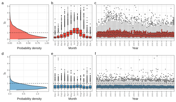
Space time metrics were calculated using Eqs. (2)–(4) and are summarized in Fig. 4 (γ2) and in Fig. S7 (γ3) by probability density, month, and year. The space time metrics for daily summertime heat index differ between γ2 (median = 1.18, range 0.03 to 6.22) and γ3 (median = 1.46, range 0.09 to 9.00). No day has a space time metric of one, but γ2 (γ3) is greater than one for 4911 (5959) days and less than one for 2817 (1769) days. Meanwhile, daily precipitation space time metrics differ between γ2 (median = 0.45, range 0.00 to 5.64) and γ3 (median = 0.57, range 0.00 to 7.19). Like heat index, no day has a space time metric of one, but γ2 (γ3) is greater than one for 2756 (4657) days and less than one for 26 903 (25 002) days. The mean and standard deviation of all daily space time metrics are reported in Fig. S8.

Figure 4Space time metrics (γ2) derived from space time separable covariance models for heat index (red) and precipitation (blue). The horizontal dashed line illustrates a space time metric of one whereby the dataset is already structured as a space time cube, which means that resampling is unnecessary for unbiased clustering. Metrics are summarized by probability density (a, d), month (b, e), and year (c, f). Heat index displays an annual pattern but there is little variability for precipitation space time metrics. Sparse outliers exist between values of 5 and 10 but were removed from plotting for clarity.
A seasonal cycle is observed when aggregating to a monthly time series of space time metrics (Fig. 4). The median space time metric for heat index is below one in the winter, spring, and autumn months (Fig. 4b) whereas the median space time metric for precipitation is consistently below one across all seasons (Fig. 4e). There is less overall variability in the precipitation space time metric (Fig. 4d) relative to heat index (Fig. 4a). The space time metrics for heat index follow an annual cycle which is greater than one in the summer (Fig. 4b) while the precipitation space time metrics lacks interannual trends besides a relative decline in the autumn (Fig. 4e). It is challenging to draw conclusions about variability in space or time because the space time metric is a ratio, such that changes may be due to changes in the numerator, denominator, or both values.
4.3 Hypothesis testing
The nonparametric Wilcoxon signed-rank test assesses whether the median difference between a sample and the test value is zero (in our case, whether the space time metric equals one). The Wilcoxon signed-rank test indicated that the median of the space time metrics is statistically significantly different from one (heat index: γ2 p < 2.02e-192, γ3 p = 0; precipitation: γ2 and γ3 p = 0) at a significance level of α = 0.05. We reject the null hypothesis that spatial and temporal distances are equivalent in ERA5-derived heat index and precipitation and find that the native ERA5 resolution is not a space time cube for either heat index or precipitation. These results indicate that resampling strategies would reduce bias in spatiotemporal clustering, which we infer would improve model performance. Figure S8 illustrates the mean ±1 standard deviation with respect to the space time metric of one to further contextualize these differences.
4.4 Clustering
4.4.1 Space time cube
We format the ERA5 data as a space time cube for each dataset using the respective median space time metric. As discussed previously, the space time metric is treated as a normalization factor to be multiplied against the native resolution to determine the resolution of the space time cube. The summertime median heat index γ2 (1.18) and γ3 (1.46) thereby converts a dataset resolved at 0.25° into a space time cube resolved at 0.30 and 0.36°, respectively. Similarly, the record median precipitation γ2 (0.45) and γ3 (0.58) would necessitate resampling into a space time cube resolved at 0.11 and 0.14°, respectively.
4.4.2 Clustering
To examine the influence of the data resolution on the weather events generated using clustering, we modelled clusters using five different resolutions. The first, 0.25°, represents the native resolution of ERA5. The remaining resolutions, 0.30 and 0.36 (0.11 and 0.14), represent the covariance-informed resolution that defines a space time cube for heat index (precipitation). Native resolution ERA5 variables were resampled using two methods: bilinear resampling estimates values at a target cell using a distance-weighted average of the surrounding native cells while maximum resampling assigns the largest value of each surrounding native cell to the target cell. In each case, resampled observations were compared against thresholds to identify extreme points suitable for clustering into extreme weather events (Figs. S1–S4).
Clustering results are described in Table 1 for the 5-year return period. Coarsening the resolution decreases the number of extreme heat events from 1621 to between 1080 and 1390. The number of extreme points decreases from 400 thousand to between 200 and 300 thousand as the resolution decreases from an 80 × 63 grid (0.25°) to 67 × 53 (0.30°, γ2) and 56 × 44 (0.36°, γ3). In addition to detecting fewer clusters, spatial coarsening results in clusters with larger extents than the native resolution of ERA5 (Fig. S9). Conversely, interpolating the resolution increases the number of extreme precipitation events from 3995 to between 5255 and 6243 (Table 1; Fig. S10). The number of extreme points increase from 160 thousand to between 510 thousand and 1.2 million as the resolution increases from an 80 × 63 grid to 182 × 143 (0.11°, γ2) and 143 × 113 (0.14°, γ2). In all cases, the number of noise points remains unchanged at 0, suggesting that the thresholds and resolutions considered in this analysis consistently result in any extreme observation being included in an extreme weather event. The annual characteristics of extreme weather events and associated trends and uncertainties are reported in Figs. S9 and S10.
Table 1Clustering results for the 5-year return period from 1940 to 2023. Outputs include the count of extreme points for clustering, the count of noise points omitted from clustering, and the count of clusters identified. Note that 0.25° represents the native ERA5 resolution all other resolutions are covariance informed.

4.5 Validation
Cluster and Iowa Environmental Mesonet datasets are reported daily by county from 2002 to 2023. Excessive heat warnings were most often reported in the states of Oklahoma and Arkansas but were rarely reported across the Appalachian Mountains (Fig. 5a). Flash flood warnings associated with extreme precipitation events are more spatially heterogeneous than for extreme heat events (Fig. 5b), occurring more frequently in more populous counties, illustrating the difference in scale between heat and precipitation events as well as their reporting frequency. Examples of each extreme weather event compared to warnings are illustrated in Figs. S11 and S12. The model skill of each resampling strategy compared to the native resolution is reported in Figs. S13–S18 and Table 2, while overall confusion matrices and recall and precision are reported in Tables S3–S6.

Figure 5The spatial count of weather warnings reported to the Iowa Environmental Mesonet between 2002 and 2023. These include (a) excessive heat warnings and (b) flash flood warnings. Warnings are reported at the county scale. Black outlines represent states while grey outlines represent NOAA County Warning Areas.
Table 2Mean F1 scores of ERA5 clusters and weather warnings across the SEUS stratified by resampling strategy and return period (RP) threshold (2002–2023). The ability for a model to perfectly reconstruct an observed dataset results in an F1 score of 1. A paired student t-test is used to quantify differences between the mean F1 scores of weather warnings and clusters at the native (0.25°) and resampled resolutions.

∗ The mean difference in F1 between the resampled and native datasets is significantly different from zero at p < 0.05.
The F1 scores for both heat index and precipitation clusters are calculated with a confusion matrix for each county in the SEUS using both the native ERA5 resolution and the covariance-informed space time cubes. Table 2 illustrates that differences in F1 scores are small but significant for most resampling strategies and thresholds. There are two exceptions to this result: no significant differences exist for precipitation clusters generated from bilinear resampling at the 5- and 10-year return periods or for the 0.14° (γ3) bilinear interpolation at the 50-year return period. Resampling heat index increases in F1 scores for each resampling strategy and return period, while bilinear (maximum) resampling precipitation decreases (increases) F1 scores, which characteristically decrease as a function of return period. However, overall, F1 scores are low across all sampling strategies for excessive heat warnings and lack any skill for flash flood warnings.
5.1 Space time metrics quantify spatiotemporal organization of heat and precipitation
We demonstrate that a covariance-informed approach for defining the space time metric enables physical interpretations of the organization of variability observed over space and time (Figs. 4 and S7). Covariance model optimization selects between single model structures when fitting experimental covariance in space but selects between single and nested model structures when fitting in time. This implies that for a given day, the physical processes controlling heat and precipitation have a single mode of variability in space (local, regional, or hemispheric extent) but either single or nested variability in time (hourly, daily, weekly and/or seasonal duration).
5.1.1 Heat index: increasing spatial coherence of summertime variability
To interpret the observed differences in spatiotemporal organization between heat index and precipitation, we evaluate space time metrics derived from space time separable covariance models fitted to hourly ERA5 fields. This metric represents the ratio of spatial to temporal variability within a given day, such that values greater than one indicates that variability is more strongly organized in space than in time, while values less than one indicate stronger temporal persistence relative to spatial coherence.
Importantly, SEUS heat extremes are frequently characterized by humid heat (i.e., elevated heat index) rather than dry-bulb temperature extremes. Humid heat events are strongly influenced by regional moisture advection from the Gulf of Mexico and western Atlantic, which tends to be spatially coherent across the domain. As a result, humid heat extremes can exhibit broader spatial footprints than dry heat extremes, even when their temporal duration remains relatively unchanged. This distinction has been shown to increase both the areal extent and intensity of heat stress in the SEUS (Diem et al., 2017; Raymond et al., 2020). The seasonal concentration of the summertime signal further supports this interpretation. From June to August, the SEUS is dominated by the western extension of the North Atlantic Subtropical High (NASH), which enhances large-scale subsidence and moisture retention (Li et al., 2011). When a positive Bermuda High displaces the NASH eastward, this regime promotes widespread warm and humid conditions, increasing spatial covariance across the region while maintaining relatively short-lived daily variability associated with diurnal cycles and transient perturbations (Bregy et al., 2025). Recent studies also suggest that declining aerosol concentrations have allowed greenhouse warming to emerge more strongly in summer, particularly in the SEUS (Leibensperger et al., 2012). In addition, research has linked SEUS humid heat extremes to tropical North Atlantic sea surface temperatures and large-scale circulation variability, further reinforcing the role of basin-scale forcing in the spatial organization of heat (Seager et al., 2009). Taken together, these findings support the interpretation of a trend toward more spatially coherent summertime humid heat regimes.
5.1.2 Precipitation: consistent spatiotemporal organization
Precipitation exhibits relatively stable spatiotemporal organization across the past several decades, with only modest changes in the space time metric (Fig. 4f). This stability is consistent with the heterogeneous mix of precipitation-generating processes in the southeastern United States. Precipitation in this region arises from a combination of mesoscale convective systems (MCSs), localized airmass and sea-breeze convection, tropical cyclones, and frontal systems. Radar-based climatologies indicate that a large fraction of warm-season precipitation is associated with organized mesoscale systems with characteristic spatial scales on the order of 102–103 km and durations of several hours (Ashley et al., 2019). At the same time, localized convection produces smaller, shorter-lived events, while frontal systems and tropical cyclones contribute longer-duration precipitation.
Changes in the frequency or intensity of these storm types do not necessarily produce systematic shifts in the ratio of spatial to temporal covariance because each spans a range of spatial and temporal scales. For example, increases in short-duration convective intensity may be offset by persistent stratiform or frontal precipitation, leading to a relatively stable aggregate space time structure. Observational studies support this interpretation, showing increases in precipitation intensity but less consistent trends in duration and frequency (Pendergrass and Hartmann, 2014; Prein and Mearns, 2021). Large-scale climate modes further modulate SEUS precipitation in a seasonally dependent manner, with the El Nino Southern Oscillation (ENSO) exerting strong control on winter precipitation and Atlantic variability influencing precipitation patterns on longer timescales (Enfield et al., 2001). Furthermore, the NASH influences moisture availability in this region: when the western ridge is located southwest (northwest) of its mean climate position, the region experiences an excess (deficit) of precipitation (Li et al., 2012), which may explain annual variability that averages out across a decadal aggregation (Fig. 4f). These competing influences can redistribute precipitation across space and time without fundamentally altering its characteristic organization.
Although long-term changes are modest, the space time metric exhibits a clear seasonal cycle, with a notable decrease in autumn (Fig. 4e), indicating a shift toward more temporally persistent precipitation. This behavior is consistent with the seasonal transition in dominant precipitation regimes. During summer, precipitation reflects a mixture of localized convection and mesoscale systems, balancing spatial and temporal covariance. In autumn, however, precipitation becomes increasingly influenced by the atmospheric low-level jet that carries warm and moist air from the Gulf of Mexico into the United States in the form of frontal systems and tropical cyclones (Kim et al., 2020). Frontal systems can produce persistent rainfall along quasi-stationary boundaries, while tropical cyclones generate prolonged precipitation along track-dependent corridors, enhancing temporal coherence without uniform spatial coverage. Recent work shows that increases in autumnal precipitation in the southeastern United States are largely driven by non-tropical frontal systems associated with enhanced Gulf moisture transport, rather than widespread increases in rainfall occurrence (Bishop et al., 2019). Together, these processes provide a physical explanation for the observed autumn decrease in the space time metric, reflecting a shift toward precipitation regimes that are temporally persistent but spatially constrained.
5.2 Spatiotemporal clustering
The smallest possible cluster contains four points, which range in three dimensions between one timestep containing four neighbouring locations (e.g., points in space) and four timesteps at a single location. Increasing the space time metric coarsens the grid over which extreme observations can be clustered, resulting in fewer clusters relative to the native grid, while decreasing the space time metric expands the grid and results in relatively more clusters (Table 1). While fewer heat index clusters are detected in both covariance-informed space time cubes, the count of clusters is a function of the grid resolution, which influences the count of extreme points that can be clustered. This in turn influences the spatial coherence of extreme weather events, where coarser grids reduce the ability for the clustering algorithm to segment exceedances into multiple events rather than one event with relatively larger extents and longer durations. This can lead to challenges while validating extreme weather events as coarser grids may result in additional False Positives when compared to higher resolution validation data. Additionally, coarser resolutions smooth out local extremes, which may explain why False Negatives are common across both types of extreme weather warnings. While these resolution limitations are shown to affect the reconstruction of excessive heat warnings, they result in a model with limited skill in delineating flash flood warnings. The scale of each type of warning gives additional support to these findings, where flash flood warnings are much more numerous (Table S1) and more often are reported in isolation (Fig. 3) than excessive heat warnings, which tend to be reported for large regions, despite infrequent reporting overall.
5.3 Validation
The choice to evaluate model performance using a confusion matrix across spatial and temporal dimensions likely results in a conservative estimate of model skill. This is due to metrics produced by a confusion matrix penalizing any discrepancies between the spatial and temporal extent of observed and modelled extreme weather events. Since the resolution of observations (county-level) is higher on average than that of ERA5 (0.25 spatial degrees), agreement between the modelled and observed extreme weather event may still yield lower than expected results because the coarser modelled event extent may induce false positive observations in neighbouring counties that did not report extreme weather. Additionally, the reporting frequency of extreme weather varies in space and time, where counties now report extreme weather more frequently than in the past, but many counties continue to underreport (or have never reported) extreme weather.
The validation of extreme heat events indicates that comparing extreme heat index clusters with excessive heat warnings produces an F1 score between 0.375 (5-year return period) and 0.389 (50-year return period) at the native ERA5 resolution (Table 2). Investigation of recall (sensitivity) and precision (Figs. S13–S15) provides an explanation for why extreme heat events are often missed but tend to be overemphasized when they are detected. Figure S13 shows that recall is moderate in the western region of the domain (mean recall = 0.412 west of 85° W) where most warnings were issued and greatest in Florida where relatively few warnings were issued (mean recall = 0.712; Fig. 5a), suggestive of greater balance between true positives and false negatives (Table S3). This implies that the clustering method identified a smaller fraction of excessive heat warnings where reporting is common, and a larger fraction where reporting is rare. Conversely, Fig. S14 illustrates that precision is greatest in the northern region of the domain (mean precision = 0.408 north of 35° N) where most warnings were issued (Fig. 5a), but low in the southern region of the domain (mean precision = 0.288 south of 35° N), suggesting relative parity between true positives and false positives (Table S3). This implies that the spatial extent of the modelled heat events may be too generous in the southern region, overestimating areas exposed to each hazard. Taken together, these spatially contrasting results for recall and precision explain moderate F1 scores across the SEUS (Fig. S15).
Improvements to model performance are marginal across all resampling and threshold definitions (Table 2), which suggest that the locally relevant hazard information necessary for skilful model performance is largely absent in ERA5 reanalysis data. While inconsistent reporting may also decrease the reported model performance, our findings provide evidence that higher resolution meteorological data would better preserve extreme observations that are otherwise smoothed in ERA5 reanalysis data, which would both increase recall by identifying and clustering more return period exceedances, and increase precision by reducing the areal extent of clustered exceedances.
Comparison between extreme precipitation clusters and flash flood warnings produces an F1 score between 0.041 (50-year return period) and 0.052 (5-year return period) at the native ERA5 resolution (Table 2). Investigation of recall (sensitivity) and precision (Figs. S16–S18) provides an explanation for why extreme precipitation events are almost never detected. Figure S16 shows that recall is essentially zero across the Southeast despite more than twice the number of warnings issued per county relative to excessive heat warnings (Fig. 5b) and a threefold greater reporting frequency than for excessive heat (Table S1), which suggests high rates of false negatives (Table S4). This implies that almost all flash flood warnings were never predicted by the clustering method, and the few warnings that are reconstructed are likely those associated with a small population of large-scale events (e.g., tropical cyclones as in Fig. S12). Conversely, Fig. S17 illustrates that precision is greater overall, especially in the western region of the domain (mean precision = 0.339 west of 85° W) where most warnings were issued (Fig. 5b), but low in the southern region of the domain, which suggests greater balance between true positives and false positives (Table S3). Overall, the low F1 scores are primarily due to an inability to reconstruct most extreme precipitation events (Fig. S18). This may be explained by the poor representation of smaller scale convective processes within coarse reanalysis products such as ERA5, thereby limiting the representation of smaller scale extreme precipitation events within our population of clusters. Ultimately, the resampling proposed here does not produce additional information, which explains why extreme weather events that do not initially appear in ERA5 continue to go unobserved. Higher resolution data may overcome this limitation by preserving extremes occurring at smaller scales. This change would likely both increase recall by identifying and clustering more return period exceedances and increase precision by reducing the areal extent of clustered exceedances.
We demonstrate that covariance-informed spatiotemporal clustering influences the number of extreme weather events observed in reanalysis data (Table 1), which greatly affects the interpretation of recent trends in hazardous weather. For example, while humid heat fluctuations are relatively coarse in space relative to time, clustering extreme heat events at such a resolution may bias results towards relatively few, longer-lasting events, even though reported excessive heat warnings suggest more modest extents and durations (Fig. S11). Conversely, precipitation fluctuations are fine in both space and time, and while clustering extreme precipitation events at such a resolution may more appropriately represent reported flash flood warnings, additional clusters that are short-lasting and spatially isolated are unlikely to be identified by simple interpolation of a coarse precipitation grid where locally isolated extremes are often attenuated.
Importantly, our results suggest that previous studies that have clustered ERA5-derived extreme heat and precipitation events at regional to global scales using the data at its native resolution (see, e.g., Liu and Zhou, 2023a; Tilloy et al., 2022) may generate different weather event sets or different weather event characteristics than if space time separable covariance modelling were to be applied to the datasets prior to clustering. For example, Tilloy et al. (2022) applied a space time metric of four when clustering extreme precipitation into weather events across the United Kingdom. This assumption makes intuitive sense as the prevalence of synoptic-scale stratiform precipitation in this region is primarily fuelled by extratropical cyclone activity, which would result in fewer observed extreme precipitation events clustered along a relatively coarser grid. However, space time separable covariance modelling would enable quantification of the magnitude of the recommended space time metric which may result in significantly fewer clusters than are currently identified, and potentially further improve model performance. An alternative approach to the hypothesis test proposed in this study is to include a buffer around the space time metric of one. Figure S8 shows the probability distribution of space time metrics overlaid with their mean and ±1 standard deviation to illustrate one possible buffering definition. In this study, such a buffer would suggest that resampling is not needed for heat index but may be important for precipitation.
Our findings for the SEUS suggest that datasets where the resolution was not checked prior to clustering should be used with caution as they may be biased in either the spatial or temporal dimension. However, we find that even after reducing bias during clustering using this approach, the subsequent events continue to poorly reconstruct hazardous conditions, especially those reported in isolation. This suggests that by defining the spatial and temporal structure of variability, the inclusion of space time separable covariance modelling into clustering frameworks marginally improves extreme weather event delineation, but that consideration of higher resolution data may yield greater improvements.
This study offers a novel empirical approach to proportionally transform spatial distances into equivalent temporal distances prior to conducting spatiotemporal clustering. We show that space time separable covariance modelling is a useful tool for understanding the scale of fluctuations of heat index and precipitation. We show that a space time metric of one indicates that a dataset is already properly formatted for spatiotemporal clustering, and that when the space time metric is not equal to one, the spatial resolution of the dataset can be scaled by this normalization factor to properly format the data. In the case study, neither heat index nor precipitation displayed a space time metric equal to one for any day in the SEUS from 1940 to 2023, suggesting that neither is a space time cube outright. While resampling each dataset into a space time cube marginally improves model skill, resulting clusters still fail to reconstruct reported extreme heat and precipitation events. This is likely because resampling strategies do not add information about local extreme observations but instead improve understanding of the number of extreme events likely to exist within the available dataset; thus, we suggest that researchers use space time metrics to assess seasonal variability in weather fluctuations, but to prefer highly resolved datasets for delineating extreme weather events.
The code used in this study is available on GitHub at https://github.com/hquintal16/cisc/tree/1.0 (last access: 16 October 2026) and linked through Zenodo (https://doi.org/10.5281/zenodo.23454977, Quintal, 2026) under an MIT license.
This analysis was conducted using R version 4.4.3, MATLAB version R2024a, and Python version 3.9.12. The meteorological datasets analysed are available through the ECMWF Reanalysis v5 (ERA5) repository, https://www.ecmwf.int/en/forecasts/dataset/ecmwf-reanalysis-v5 (last access: 17 April 2024). NOAA NWS WFO CWA shapefiles are available through the NWS online GIS portal, https://www.weather.gov/gis/CWABounds (last access: 4 April 2026). Weather warnings are available in the Iowa Environmental Mesonet NWS repository, https://mesonet.agron.iastate.edu/vtec/search.php?mode=bypoint (last access: 9 July 2026). Environmental Protection Agency (EPA) Ecoregion shapefiles are available through the National Aquatic Resources Survey, https://www.epa.gov/national-aquatic-resource-surveys/ecoregions-used-national-aquatic-resource-surveys (last access: 4 April 2026). BMElib software is available in the BMElib repository, https://mserre.sph.unc.edu/BMElib_web/ (last access: 26 September 2022).
The supplement related to this article is available online at https://doi.org/10.5194/hess-30-7083-2026-supplement.
H.Q.: Conceptualization; Data curation; Formal analysis; Investigation; Methodology; Software; Validation; Visualization; Writing – original draft preparation; Writing – review and editing. A.S.: Conceptualization; Funding acquisition; Resources; Methodology; Supervision; Validation; Visualization; Writing – original draft preparation; Writing – review and editing. M.S.: Conceptualization; Resources; Methodology; Software; Supervision; Writing – review and editing. W.J.: Conceptualization; Methodology; Writing – review and editing. M.C.R.: Resources; Writing – review and editing.
At least one of the (co-)authors serves as associate editor for the “Methodological innovations for the analysis and management of compound risk and multi-risk, including climate-related and geophysical hazards (NHESS/ESD/ESSD/GC/HESS inter-journal SI)” to which this paper belongs. The peer-review process was guided by an independent editor, and the authors also have no other competing interests to declare.
NOAA had no role in the design or conduct of the study; data analysis or interpretation; preparation, review, or approval of the manuscript; or decision to submit the manuscript for publication.
Publisher's note: Copernicus Publications remains neutral with regard to jurisdictional claims made in the text, published maps, institutional affiliations, or any other geographical representation in this paper. The authors bear the ultimate responsibility for providing appropriate place names. Views expressed in the text are those of the authors and do not necessarily reflect the views of the publisher.
This article is part of the special issue “Methodological innovations for the analysis and management of compound risk and multi-risk, including climate-related and geophysical hazards (NHESS/ESD/ESSD/GC/HESS inter-journal SI)”. It is not associated with a conference.
We thank the Myriad-EU project at Vrije Universiteit Amsterdam for hosting Hunter Quintal as a visiting researcher during the summer of 2024. We thank members of the Myriad-EU project for constructive discussions, especially Davide Ferrario, Kelley de Polt, Judith Claassen, and Sophie Buijs. We acknowledge the use of Artificial Intelligence (AI) in assisting in the development of R code for the analysis (ChatGPT version 5).
This study was supported in part by a grant from the National Oceanic and Atmospheric Administration (NOAA) Climate Program Office Regional Integrated Sciences and Assessments program: Modernizing Risk Assessment for High-Impact Weather Events in the Carolinas (2021–2026) [NA21OAR4310312]. MCR and WJ also received funding from the MYRIAD-EU project, which received funding from the European Union's Horizon 2020 research and innovation programme under grant agreement no. 101003267. MCR also received support from the Netherlands Organisation for Scientific Research (NOW) (VENI; grant no. VI. Veni.222.169).
This paper was edited by Aloïs Tilloy and reviewed by two anonymous referees.
Agrawal, K. P., Garg, S., Sharma, S., and Patel, P.: Development and validation of OPTICS based spatio-temporal clustering technique, Inf. Sci. (N.Y.), 369, 388–401, https://doi.org/10.1016/j.ins.2016.06.048, 2016.
Agulles, M., Marcos, M., Amores, A., and Toomey, T.: Storm surge modelling along European coastlines: The effect of the spatio-temporal resolution of the atmospheric forcing, Ocean Model. (Oxf.), 192, https://doi.org/10.1016/j.ocemod.2024.102432, 2024.
Alvera-Azcárate, A., Barth, A., Beckers, J.-M., and Weisberg, R. H.: Multivariate reconstruction of missing data in sea surface temperature, chlorophyll, and wind satellite fields, J. Geophys. Res.-Oceans, 112, https://doi.org/10.1029/2006JC003660, 2007.
Ansari, M., Ahmad, A., Khan, S., Bhushan, G., and Mainuddin: Spatiotemporal clustering: a review, Artif. Intell. Rev., 53, 2381–2423, https://doi.org/10.1007/s10462-019-09736-1, 2020.
Ashley, W. S., Haberlie, A. M., and Strohm, J.: A climatology of quasi-linear convective systems and their hazards in the united states, Weather Forecast., 34, 1605–1631, https://doi.org/10.1175/WAF-D-19-0014.1, 2019.
Bach, B., Dragicevic, P., Archambault, D., Hurter, C., and Carpendale, S.: A Descriptive Framework for Temporal Data Visualizations Based on Generalized Space-Time Cubes, Computer Graphics Forum, 36, 36–61, https://doi.org/10.1111/cgf.12804, 2017.
Barbero, R., Fowler, H. J., Blenkinsop, S., Westra, S., Moron, V., Lewis, E., Chan, S., Lenderink, G., Kendon, E., Guerreiro, S., Li, X. F., Villalobos, R., Ali, H., and Mishra, V.: A synthesis of hourly and daily precipitation extremes in different climatic regions, Weather Clim. Extrem., 26, https://doi.org/10.1016/j.wace.2019.100219, 2019.
Birant, D. and Kut, A.: ST-DBSCAN: An algorithm for clustering spatial-temporal data, Data Knowl. Eng., 60, 208–221, https://doi.org/10.1016/j.datak.2006.01.013, 2007.
Bishop, D. A., Williams, A. P., and Seager, R.: Increased Fall Precipitation in the Southeastern United States Driven by Higher-Intensity, Frontal Precipitation, Geophys. Res. Lett., 46, 8300–8309, https://doi.org/10.1029/2019GL083177, 2019.
Bregy, J. C., Maxwell, J. T., Robeson, S. M., Harley, G. L., and Trouet, V.: Changes in the western flank of the North Atlantic subtropical high since 1140 CE: Extremes, drivers, and hydroclimatic patterns, Sci. Adv., 11, 1–11, 2025.
Cammalleri, C. and Toreti, A.: A Generalized Density-Based Algorithm for the Spatiotemporal Tracking of Drought Events, J. Hydrometeorol., 24, 537–548, https://doi.org/10.1175/JHM-D-22-0115.1, 2023.
Christakos, G.: A Bayesian/Maximum-Entropy View to the Spatial Estimation Problem, Math. Geol., 22, 763–777, 1990.
Christakos, G. and Li, X.: Bayesian Maximum Entropy Analysis and Mapping: A Farewell to Kriging Estimators?, Math. Geol., 30, 435–462, https://doi.org/10.1023/A:1021748324917, 1998.
Christakos, G. and Serre, M.: BME analysis of spatiotemporal particulate matter distributions in North Carolina, Atmos. Environ., 34, 3393–3406, 1999.
Christakos, G., Hristopulos, D., and Bogaert, P.: On the physical geometry concept at the basis of space/time geostatistical hydrology, Adv. Water Resour., 23, 799–810, 2000.
Christakos, G., Bogaert, P., and Serre, M.: Temporal GIS: advanced functions for field-based applications, Springer Science & Business Media, https://doi.org/10.1007/978-3-642-56540-3, 2002.
Christakos, G., Angulo, J. M., Yu, H. L., and Wu, J.: Space-time metric determination in environmental modeling, J. Environ. Inform., 30, 29–40, https://doi.org/10.3808/jei.201700365, 2017.
Delang, M., Becker, J., Chang, K., Serre, M., Cooper, O., Schultz, M., Schröder, S., Lu, X., Zhang, L., Deushi, M., Josse, B., Keller, C., Lamarque, J., Lin, M., Liu, J., Marécal, V., Strode, S., Sudo, K., Tilmes, S., Zhang, L., Cleland, S., Collins, E., Brauer, M., and West, J.: Mapping Yearly Fine Resolution Global Surface Ozone through the Bayesian Maximum Entropy Data Fusion of Observations and Model Output for 1990–2017, Environ. Sci. Technol., 55, 4389–4398, https://doi.org/10.1021/acs.est.0c07742, 2021.
Dey, R. and Chakraborty, S.: Convex-Hull & DBSCAN Clustering to Predict Future Weather, in: 2015 International Conference and Workshop on Computing and Communication (IEMCON), 1–8, https://doi.org/10.1109/IEMCON.2015.7344438, 2015.
Di Napoli, C., Pappenberger, F., and Cloke, H.: Verification of Heat Stress Thresholds for a Health-Based Heat-Wave Definition, J. Appl. Meteorol. Clim., 58, 1177–1194, https://doi.org/10.1175/JAMC-D-18-0246.1, 2019.
Diem, J., Stauber, C., and Rothenberg, R.: Heat in the southeastern United States: Characteristics, trends, and potential health impact, PLOS ONE, 12, https://doi.org/10.1371/journal.pone.0177937, 2017.
Drakes, O., Tate, E., Rainey, J., and Brody, S.: Social vulnerability and short-term disaster assistance in the United States, Int. J. Disast. Risk Re., 53, https://doi.org/10.1016/j.ijdrr.2020.102010, 2021.
Enfield, D. B., Mestas-Nuñez, A. M., and Trimble, P. J.: The Atlantic multidecadal oscillation and its relation to rainfall and river flows in the continental U.S, Geophys. Res. Lett., 28, 2077–2080, https://doi.org/10.1029/2000GL012745, 2001.
Ester, M., Kriegel, H.-P., Sander, J., and Xu, X.: A Density-Based Algorithm for Discovering Clusters in Large Spatial Databases with Noise, in: Proceedings of the Second International Conference on Knowledge Discovery and Data Mining, 226–231, 1996.
Fox, L., Serre, M., Lippmann, S., Rodríguez, D., Bangdiwala, S., Gutiérrez, M., Escobar, G., and Villaveces, A.: Spatiotemporal Approaches to Analyzing Pedestrian Fatalities: The Case of Cali, Colombia, Traffic Inj. Prev., 16, 571–577, https://doi.org/10.1080/15389588.2014.976336, 2015.
Gómez, A., Serre, M., Wise, E., and Pavelsky, T.: Integrating Community Science Research and Space-Time Mapping to Determine Depth to Groundwater in a Remote Rural Region, Water Resour. Res., 57, https://doi.org/10.1029/2020WR029519, 2021.
Hahsler, M., Piekenbrock, M., and Doran, D.: Dbscan: Fast density-based clustering with R, J. Stat. Softw., 91, https://doi.org/10.18637/jss.v091.i01, 2019.
Hassler, B. and Lauer, A.: Comparison of reanalysis and observational precipitation datasets including era5 and wfde5, Atmosphere-Basel, 12, https://doi.org/10.3390/atmos12111462, 2021.
Hersbach, H., Bell, B., Berrisford, P., Hirahara, S., Horányi, A., Muñoz-Sabater, J., Nicolas, J., Peubey, C., Radu, R., Schepers, D., Simmons, A., Soci, C., Abdalla, S., Abellan, X., Balsamo, G., Bechtold, P., Biavati, G., Bidlot, J., Bonavita, M., de Chiara, G., Dahlgren, P., Dee, D., Diamantakis, M., Dragani, R., Flemming, J., Forbes, R., Fuentes, M., Geer, A., Haimberger, L., Healy, S., Hogan, R. J., Hólm, E., Janisková, M., Keeley, S., Laloyaux, P., Lopez, P., Lupu, C., Radnoti, G., de Rosnay, P., Rozum, I., Vamborg, F., Villaume, S., and Thépaut, J. N.: The ERA5 global reanalysis, Q. J. Roy. Meteor. Soc., 146, 1999–2049, https://doi.org/10.1002/qj.3803, 2020.
Holcomb, D., Messier, K., Serre, M., Rowny, J., and Stewart, J.: Geostatistical Prediction of Microbial Water Quality Throughout a Stream Network Using Meteorology, Land Cover, and Spatiotemporal Autocorrelation, Environ. Sci. Technol., 52, 7775–7784, https://doi.org/10.1021/acs.est.8b01178, 2018.
Hüsch, M., Schyska, B. U., and von Bremen, L.: CorClustST—Correlation-based clustering of big spatio-temporal datasets, Future Gener. Comp. Sy., 110, 610–619, https://doi.org/10.1016/j.future.2018.04.002, 2020.
Iglesias, V., Braswell, A. E., Rossi, M. W., Joseph, M. B., McShane, C., Cattau, M., Koontz, M. J., McGlinchy, J., Nagy, R. C., Balch, J., Leyk, S., and Travis, W. R.: Risky Development: Increasing Exposure to Natural Hazards in the United States, Earths Future, 9, https://doi.org/10.1029/2020EF001795, 2021.
KC, B., Shepherd, J. M., King, A. W., and Johnson Gaither, C.: Multi-hazard climate risk projections for the United States, Nat. Hazards, 105, 1963–1976, https://doi.org/10.1007/s11069-020-04385-y, 2021.
Kidd, C., Becker, A., Huffman, G., Muller, C., Joe, P., Skofronick-Jackson, G., and Kirschbaum, D.: So, how much of the Earth's surface is covered by rain gauges?, B. Am. Meteorol. Soc., 98, 69–78, https://doi.org/10.1175/BAMS-D-14-00283.1, 2017.
Kim, D., Lee, S. K., Lopez, H., Foltz, G. R., Misra, V., and Kumar, A.: On the Role of Pacific-Atlantic SST Contrast and Associated Caribbean Sea Convection in August–October U. S. Regional Rainfall Variability, Geophys. Res. Lett., 47, https://doi.org/10.1029/2020GL087736, 2020.
Kisilevieh, S., Mansmann, F., Nanni, M., and Rinzivillo, S.: Spatio-temporal clustering, Data Mining and Knowledge Discovery Handbook, 2nd edn., Springer, New York, 1, 855–874, 2010.
Kolovos, A., Christakos, G., Hristopulos, D., and Serre, M.: Methods for generating non-separable spatiotemporal covariance models with potential environmental applications, Adv. Water Resour., 27, 815–830, https://doi.org/10.1016/j.advwatres.2004.04.002, 2004.
Lamb, D. S., Downs, J., and Reader, S.: Space-time hierarchical clustering for identifying clusters in spatiotemporal point data, ISPRS Int. J. Geoinf., 9, https://doi.org/10.3390/ijgi9020085, 2020.
Leibensperger, E. M., Mickley, L. J., Jacob, D. J., Chen, W.-T., Seinfeld, J. H., Nenes, A., Adams, P. J., Streets, D. G., Kumar, N., and Rind, D.: Climatic effects of 1950–2050 changes in US anthropogenic aerosols – Part 1: Aerosol trends and radiative forcing, Atmos. Chem. Phys., 12, 3333–3348, https://doi.org/10.5194/acp-12-3333-2012, 2012.
Li, L., Li, W., and Kushnir, Y.: Variation of the North Atlantic subtropical high western ridge and its implication to Southeastern US summer precipitation, Clim. Dynam., 39, 1401–1412, https://doi.org/10.1007/s00382-011-1214-y, 2012.
Li, W., Li, L., Fu, R., Deng, Y., and Wang, H.: Changes to the North Atlantic subtropical high and its role in the intensification of summer rainfall variability in the southeastern United States, J. Climate, 24, 1499–1506, https://doi.org/10.1175/2010JCLI3829.1, 2011.
Li, X., Plale, B., Vijayakumar, N., Ramachandran, R., Graves, S., and Conover, H.: Real-time storm detection and weather forecast activation through data mining and events processing, Earth Sci. Inform., 1, 49–57, https://doi.org/10.1007/s12145-008-0010-7, 2008a.
Li, X., Ramachandran, R., Movva, S., Graves, S., Plale, B., and Vijayakumar, N.: Storm Clustering for Data-driven Weather Forecasting, in: 24th Conference on International Institute of Professional Studies (IIPS), 2008b.
Liu, Z. and Zhou, W.: Glo3DHydroClimEventSet(v1.0): A global-scale event set of hydroclimatic extremes detected with the 3D DBSCAN-based workflow (1951–2022), Int. J. Climatol., 43, 7722–7744, https://doi.org/10.1002/joc.8289, 2023a.
Liu, Z. and Zhou, W.: Global Seasonal-Scale Meteorological Droughts. Part I: Detection, Metrics, and Inland/Coastal Types, Ocean-Land-Atmosphere Research, 2, https://doi.org/10.34133/olar.0016, 2023b.
Luo, M., Lau, N., Liu, Z., Wu, S., and Wang, X.: An Observational Investigation of Spatiotemporally Contiguous Heatwaves in China From a 3D Perspective, Geophys. Res. Lett., 49, https://doi.org/10.1029/2022GL097714, 2022.
Oliveira, R., Santos, M. Y., and Pires, J. M.: 4D+SNN: A spatio-temporal density-based clustering approach with 4D similarity, in: Proceedings – IEEE 13th International Conference on Data Mining Workshops, ICDMW 2013, 1045–1052, https://doi.org/10.1109/ICDMW.2013.119, 2013.
Paprotny, D., Sebastian, A., Morales-Nápoles, O., and Jonkman, S.: Trends in flood losses in Europe over the past 150 years, Nat. Commun., 9, https://doi.org/10.1038/s41467-018-04253-1, 2018.
Paprotny, D., Rhein, B., Vousdoukas, M. I., Terefenko, P., Dottori, F., Treu, S., Śledziowski, J., Feyen, L., and Kreibich, H.: Merging modelled and reported flood impacts in Europe in a combined flood event catalogue for 1950–2020, Hydrol. Earth Syst. Sci., 28, 3983–4010, https://doi.org/10.5194/hess-28-3983-2024, 2024.
Pasche, O. C., Wider, J., Zhang, Z., Zscheischler, J., and Engelke, S.: Validating Deep Learning Weather Forecast Models on Recent High-Impact Extreme Events, Artificial Intelligence for the Earth Systems, 4, 1–24, https://doi.org/10.1175/AIES-D-24-0033.1, 2025.
Pendergrass, A. G. and Hartmann, D. L.: Changes in the Distribution of Rain Frequency and Intensity in Response to Global Warming, J. Climate, 27, 8372–8383, https://doi.org/10.1175/JCLI-D-14-00183.s1, 2014.
Polasky, A., Sapkota, V., Forest, C., and Fuentes, J.: Discrepancies in precipitation trends between observational and reanalysis datasets in the Amazon Basin, Sci. Rep., 15, https://doi.org/10.1038/s41598-025-87418-5, 2025.
Prein, A. F. and Mearns, L. O.: U.S. Extreme Precipitation Weather Types Increased in Frequency During the 20th Century, J. Geophys. Res.-Atmos., 126, https://doi.org/10.1029/2020JD034287, 2021.
Quintal, H.: Code repository for Covariance-informed spatiotemporal clustering improves the detection of hazardous weather events, Version 1.0, Zenodo [computer software], https://doi.org/10.5281/zenodo.23454977, 2026.
Racah, E., Beckham, C., Maharaj, T., Kahou, S. E., Prabhat, and Pal, C.: ExtremeWeather: A large-scale climate dataset for semi-supervised detection, localization, and understanding of extreme weather events, arXiv [preprint], https://doi.org/10.48550/arXiv.1612.02095, 2017.
Raymond, C., Matthews, T., and Horton, R.: The emergence of heat and humidity too severe for human tolerance, Sci. Adv., 8, 1–8, https://doi.org/10.1126/sciadv.aaw1838, 2020.
Raymond, C., Matthews, T., Horton, R., Fischer, E., Fueglistaler, S., Ivanovich, C., Suarez-Gutierrez, L., and Zhang, Y.: On the Controlling Factors for Globally Extreme Humid Heat, Geophys. Res. Lett., 48, https://doi.org/10.1029/2021GL096082, 2021.
Raymond, C., Waliser, D., Guan, B., Lee, H., Loikith, P., Massoud, E., Sengupta, A., Singh, D., and Wootten, A.: Regional and elevational patterns of extreme heat stress change in the US, Environ. Res. Lett., 17, https://doi.org/10.1088/1748-9326/ac7343, 2022.
Reidmiller, D., Avery, C., Easterling, D., Kunkel, K., and Lewis, K.: Impacts, Risks, and Adaptation in the United States: Fourth National Climate Assessment, Volume II, edited by: Reidmiller, D. R., Avery, C. W., Easterling, D. R., Kunkel, K. E., Lewis, K. L. M., Maycock, T. K., and Stewart, B. C., U.S. Global Change Research Program, Washington, DC, USA, 1506 pp., https://doi.org/10.7930/NCA4.2018, 2018.
Reynolds, A. P., Richards, G., de La Iglesia, B., and Rayward-Smith, V. J.: Clustering rules: A comparison of partitioning and hierarchical clustering algorithms, Journal of Mathematical Modelling and Algorithms, 5, 475–504, https://doi.org/10.1007/s10852-005-9022-1, 2006.
Rogers, C., Ting, M., Li, C., Kornhuber, K., Coffel, E., Horton, R., Raymond, C., and Singh, D.: Recent Increases in Exposure to Extreme Humid-Heat Events Disproportionately Affect Populated Regions, Geophys. Res. Lett., 48, https://doi.org/10.1029/2021GL094183, 2021.
Rogers, C., Kornhuber, K., Perkins-Kirkpatrick, S., Loikith, P., and Sinhg, D.: Sixfold Increase in Historical Northern Hemisphere Concurrent Large Heatwaves Driven by Warming and Changing Atmospheric Circulations, J. Climate, 35, 1063–1078, https://doi.org/10.1175/JCLI-D-21-0200.s1, 2022.
Rothfusz, L. P.: The Heat Index “Equation” (or, More Than You Ever Wanted to Know About Heat Index), Fort Worth, NWS Southern Region Headquarters, 1–2, https://www.weather.gov/media/ffc/ta_htindx.PDF (last access: 23 February 2026), 1990.
Rus, A. M. M., Othman, Z. A., Bakar, A. A., and Zainudin, S.: A Hierarchical ST-DBSCAN with Three Neighborhood Boundary Clustering Algorithm for Clustering Spatio–temporal Data, International Journal of Advanced Computer Science and Applications, 13, 614–626, https://doi.org/10.14569/IJACSA.2022.0131274, 2022.
Saltikoff, E., Friedrich, K., Soderholm, J., Lengfeld, K., Nelson, B., Becker, A., Hollmann, R., Urban, B., Heistermann, M., and Tassone, C.: An overview of using weather radar for climatological studies successes, challenges, and potential, 100, 1739–1752, https://doi.org/10.1175/BAMS-D-18-0166.1, 2019.
Seager, R., Tzanova, A., and Nakamura, J.: Drought in the Southeastern United States: Causes, variability over the last millennium, and the potential for future hydroclimate change, J. Climate, 22, 5021–5045, https://doi.org/10.1175/2009JCLI2683.1, 2009.
Serre, M. and Bogaert, P.: The Bayesian Maximum Entropy software for Space/Time Geostatistics, and temporal GIS data integration, https://mserre.sph.unc.edu/BMElib_web/ (last access: 26 October 2026), 2009.
Serre, M. L. and Christakos, G.: Modern geostatistics: computational BME analysis in the light of uncertain physical knowledge ± the Equus Beds study, Stoch. Env. Res. Risk A., 13, 1–26, 1999.
Summers, J. K., Lamper, A., McMillion, C., and Harwell, L. C.: Observed Changes in the Frequency, Intensity, and Spatial Patterns of Nine Natural Hazards in the United States from 2000 to 2019, Sustainability (Switzerland), 14, https://doi.org/10.3390/su14074158, 2022.
Terando, A., Costanza, J., Belyea, C., Dunn, R., and Mckerrow, A.: The Southern Megalopolis: Using the Past to Predict the Future of Urban Sprawl in the Southeast, PLOS ONE, 9, 102261, https://doi.org/10.1371/journal.pone.0102261, 2014.
Tierney, G. E., Mallard, M. S., Spero, T. L., and Jalowska, A. M.: A novel framework for expanding temperature intensity-duration-frequency curve utility, Nat. Hazards, 122, https://doi.org/10.1007/s11069-025-07811-1, 2026.
Tilloy, A., Malamud, B. D., and Joly-Laugel, A.: A methodology for the spatiotemporal identification of compound hazards: wind and precipitation extremes in Great Britain (1979–2019), Earth Syst. Dynam., 13, 993–1020, https://doi.org/10.5194/esd-13-993-2022, 2022.
Tin Tin, T., Jia Hao, Y., Chang Yeou, Y., Siew Mooi, L., Ting Yew, G., Olumide Olugbade, T., and Aitizaz, A.: Natural Disaster Clustering Using K-Means, DBSCAN, SOM, GMM, and Mean Shift: An Analysis of Fema Disaster Statistics, IJACSA) International Journal of Advanced Computer Science and Applications, 15, 667–681, https://doi.org/10.14569/IJACSA.2024.0150968, 2024.
Wang, M., Wang, A., and Li, A.: Mining Spatial-temporal Clusters from Geo-databases, International Journal of Advanced Data Mining and Applications, 4093, 263–270, https://doi.org/10.1007/11811305_29, 2006.
Ward, P. J., Blauhut, V., Bloemendaal, N., Daniell, J. E., de Ruiter, M. C., Duncan, M. J., Emberson, R., Jenkins, S. F., Kirschbaum, D., Kunz, M., Mohr, S., Muis, S., Riddell, G. A., Schäfer, A., Stanley, T., Veldkamp, T. I. E., and Winsemius, H. C.: Review article: Natural hazard risk assessments at the global scale, Nat. Hazards Earth Syst. Sci., 20, 1069–1096, https://doi.org/10.5194/nhess-20-1069-2020, 2020.
Wibisono, S., Anwar, M., Supriyanto, A., and Amin, I. H.: Multivariate weather anomaly detection using DBSCAN clustering algorithm, J. Phys. Conf. Ser., 1869, 012077, https://doi.org/10.1088/1742-6596/1869/1/012077, 2021.
Yin, C., Ting, M., Kornhuber, K., Horton, R. M., Yang, Y., and Jiang, Y.: CETD, a global compound events detection and visualisation toolbox and dataset, Sci. Data, 12, https://doi.org/10.1038/s41597-025-04530-x, 2025.