
the Creative Commons Attribution 4.0 License.
the Creative Commons Attribution 4.0 License.
 | 16 Nov 2026
Testing the temporal and spatial transferability of a water balance model using a parameter learning approach

François Bourgin
Charles Perrin
Vazken Andréassian
Reliable transferability of hydrological model parameters across time and space remains a challenge for large-scale water resources assessment. In this study, we investigate whether a differentiable hybrid framework can identify robust and physically coherent parameter sets for annual streamflow modeling across a large-sample dataset of 3044 catchments from eight countries. To focus on temporal and spatial transferability analysis, we work at the annual time scale using what we consider to be the simplest possible model: an annual anomaly model of climate elasticities, coupled with the Turc–Mezentsev formulation for the long-term streamflow mean (MQ). A dense neural network is trained in an end-to-end fashion to map catchment descriptors to the four model parameters: because the anomaly-model equations are fully differentiable with respect to their parameters, the gradients of the streamflow loss are backpropagated through these equations to the neural network weights.
We evaluate the framework using three cross-validation settings inspired by Klemeš (1986): temporal, spatial, and combined temporal–spatial cross-validation. As a benchmark, we compare the hybrid model against local, catchment-by-catchment linear regressions under temporal cross-validation.
Our results show that, for temporal transferability, our parameter learning approach outperforms local calibration, yielding higher Nash-Sutcliffe efficiency (NSE) values while producing elasticity coefficients that remain within plausible physical ranges, despite lacking explicit parameter constraints. By contrast, spatial transferability reveals a marked limitation: the anomaly component extrapolates well spatially, but regionalizing MQ from descriptors proves difficult, with MQ errors dominating the loss of performance in spatial and spatiotemporal cross-validation. Experiments with random descriptors further show that our parameter learning uses attributes mainly as catchment identifiers in temporal cross-validation but relies on their physical content to sustain spatial transfer, particularly for MQ. Overall, the study demonstrates that simple differentiable hybrid annual models can learn robust and interpretable anomaly parameters, while highlighting MQ regionalization as the main remaining bottleneck for spatially transferable annual streamflow predictions.
- Article
(5366 KB) - Full-text XML
-
Supplement
(328 KB) - BibTeX
- EndNote


1.1 Parameter transferability across space and time: strategies and limitations
Most hydrologists agree that a hydrological model's ability to extrapolate under changing conditions is fundamental, whether for effective management of water resources, the design of hydraulic infrastructure, or the implementation of ecosystem services (de Lavenne et al., 2019; Parajka et al., 2013). This property, however, has yet to be achieved and remains among the unsolved problems in hydrology, as compiled by Blöschl et al. (2019): “How can hydrological models be adapted to be able to extrapolate to changing conditions?” It is primarily defined by two dimensions of transferability: spatial transferability, also known as “prediction in ungauged basins” (PUB), which seeks to provide predictions where no discharge records exist, and temporal transferability, which challenges a model's ability to maintain its predictive performance under changing climatic conditions (Blöschl et al., 2019; Klemeš, 1986). While the International Association of Hydrological Sciences (IAHS) PUB decade (Sivapalan et al., 2003) and the subsequent “Panta Rhei” initiative (Montanari et al., 2013) have significantly advanced these topics (Hrachowitz et al., 2013), identifying robust parameter sets that can bridge the gap between regional information and ungauged locations while remaining stable across different hydroclimatic periods remains a critical research frontier (Rojas-Serna et al., 2016; Santos et al., 2025).
To overcome the lack of local data, hydrologists have developed regionalization strategies to transfer information from gauged “donor” catchments to “receiver” ungauged ones (McIntyre et al., 2005; Oudin et al., 2010; Parajka et al., 2013). These classic approaches rely on three main pillars:
-
Regression-based methods, linking model parameters to physical or climatic descriptors (e.g., Seibert, 1999);
-
Physical similarity-based methods, transferring parameters between catchments sharing similar physical attributes such as slope, aridity, or land cover (e.g., Ali et al., 2012; Heng and Suetsugi, 2014; McIntyre et al., 2005; Wolock et al., 2004);
-
Spatial proximity-based methods, assuming that neighboring basins behave similarly due to shared climate and geology (e.g., Kim and Kaluarachchi, 2008; Merz and Blöschl, 2004; Parajka et al., 2005).
The effectiveness of regionalization strategies is highly dependent on the density of the stream gauge network (Heng and Suetsugi, 2014; Lebecherel et al., 2016). In regions characterized by a dense network of gauging stations, approaches based on spatial proximity consistently outperform other methods; France and Australia are often used as examples in this context (Merz and Blöschl, 2004; Oudin et al., 2008), although they are by no means the only countries with dense networks. However, this superiority is sensitive to data availability: in areas with sparse hydrometric networks and distant gauging stations, physical similarity can outperform spatial proximity (Heng and Suetsugi, 2014; Parajka et al., 2013). Lastly, comparative assessments indicate that regression-based methods yield the lowest performance (Oudin et al., 2008; Parajka et al., 2013; Razavi and Coulibaly, 2013), underscoring the need to handle complete parameter sets.
On the temporal dimension, model stability is typically achieved through structural choices and specific parameterization schemes. Model parsimony is frequently advocated as a primary way to address over-parameterization, thereby enhancing the stability of parameter sets when applied to periods beyond calibration (Perrin et al., 2001). Other strategies include the use of dynamic parameterization, which allows models to adapt to changing regimes (Lan et al., 2020; Stephens et al., 2019). Furthermore, the concept of “discrete parameterization” through parameter set libraries has been proposed to provide more stable results than local calibration, especially when data are limited or when models face non-stationary conditions (Andréassian et al., 2014; Perrin et al., 2008).
The evaluation of a model's extrapolation ability requires rigorous protocols (Refsgaard and Henriksen, 2004). The international benchmark remains the hierarchical scheme proposed by Klemeš (1986), which defines the Split-Sample Test (SST) for temporal validity and the Proxy-Basin Test (PBT) for spatial transposability. Specifically, the Differential Split-Sample Test (DSST) challenges the model by evaluating parameters over contrasting climatic periods (Klemeš, 1986; Seibert, 2003). These protocols are often described as “crash tests”, essential for detecting failures outside the model's historical calibration range (Andréassian et al., 2009). At the same time, recent studies have shown that standard split-sample implementations can sometimes give an unduly pessimistic view of model robustness, by missing parameter sets that perform satisfactorily across different climatic periods (Fowler et al., 2016), and have proposed more systematic frameworks to diagnose whether failures under changing conditions stem from structural inadequacy, parameterization issues, or data errors (Fowler et al., 2018).
Despite decades of development and refinement, traditional hydrological models face fundamental structural limitations because they are often over-simplified representations, plagued by structural deficiencies, and unable to handle all hydrological processes. For instance, many conceptual structures lack explicit vegetation modules (such as seasonally varying leaf area index or rooting depth) or struggle to capture multi-year hydrological memory and complex groundwater interactions (Feng et al., 2022; Grigg and Hughes, 2018).
These structural gaps often lead to parameter identification issues. When a model structure is imperfect, the calibration process often forces parameters to vary in non-sensical ways to compensate for missing physics or data biases (Kirchner, 2006). While equifinality (the existence of multiple and disparate parameter sets yielding identical fits) is a well-known challenge (Beven, 2006), its impact is particularly acute in conceptual models, rendering objective relationship between parameters and physical catchment characteristics elusive (Oudin et al., 2010). This results in a lack of temporal robustness, where parameter sets calibrated during wet periods fail to reproduce dry periods, and vice versa (Merz et al., 2011; Vaze et al., 2010). Because these models often act as “mathematical marionettes” that can only “dance to a tune they have already heard” (Kirchner, 2006), they frequently fail climatic “crash tests” when facing conditions beyond their historical calibration range (Coron et al., 2012). This highlights the need for modeling architectures capable of learning missing processes from big data while maintaining fundamental physical consistencies (Jiang et al., 2020).
1.2 Beyond regional calibration: a new hybrid paradigm
In an attempt to address the limitations of traditional conceptual models, part of the hydrological community has recently begun exploring possible synergies between physical process-based models and deep learning (Jiang et al., 2020; Reichstein et al., 2019; Shen, 2018). This hybrid paradigm seeks to overcome the dichotomy between the high predictive accuracy of “black-box” machine learning models and the interpretability of physical–conceptual structures (Höge et al., 2022; Jiang et al., 2020). By utilizing a physical backbone, such as the HBV (Bergström, 1976) or the GR (Perrin et al., 2003) models, these hybrid structures ensure mass conservation and physical consistency while leveraging the data-driven flexibility of deep learning (Feng et al., 2022; Huynh et al., 2024). These models can effectively compensate for structural deficiencies or missing processes by outsourcing them to learnable components, thereby matching the performance of state-of-the-art pure deep learning models while providing access to internal physical fluxes such as baseflow and evapotranspiration (Feng et al., 2022; Jiang et al., 2020).
A major breakthrough in the field of hybrid modeling comes from the adoption of differentiable programming (Shen et al., 2023), a computing paradigm that allows for gradient tracking through every operation in the model pipeline (Paszke et al., 2019). This enables a differentiable parameter learning (dPL) framework in which a neural network is trained to map raw catchment attributes directly to hydrological model parameters (Feng et al., 2022; Tsai et al., 2021). In this sense, dPL represents a modern, deep-learning-based evolution of regional calibration strategies. While traditional regional calibration often relies on rigid, human-designed transfer functions or regional pooling to find common parameter sets (e.g., Poncelet, 2016), the dPL approach facilitates learning these complex mappings using all available data simultaneously. Unlike traditional local calibration, which fits a separate model to each basin and often results in disparate or sometimes “pathological” parameter sets, dPL leverages the scaling effects of big data to identify generic relationships across thousands of catchments (Tsai et al., 2021).
In this framework, the neural network is constrained by the process-based backbone, ensuring that the learned mapping respects physical laws such as mass conservation (Acuña Espinoza et al., 2024; Feng et al., 2022). This structural constraint restricts the learnable functional space to a physically permissible subspace, ensuring that the model's outputs remain hydrologically consistent even when the internal neural network is highly flexible. Furthermore, by training the model on a large set of catchments, the system is forced to identify generic signals shared across regions. This helps mitigate the risk of overfitting to site-specific noise or local data errors that typically plague site-by-site calibration. This synergy between physical consistency and global learning favors the identification of physically coherent parameter sets that are more likely to remain valid under changing climatic conditions (Feng et al., 2022; Tsai et al., 2021).
1.3 Why use a parsimonious annual anomaly and water balance model?
In the context of water resources management and policy planning, the choice of an appropriate level of model complexity is a critical decision that directly impacts the reliability of long-term assessments. While daily conceptual models are widely used, adopting a parsimonious annual anomaly model is strategically justified both by the nature of the information contained in hydrometeorological records and by the specific requirements of large-scale resource estimation.
Simulating hydrological behavior across large geographic domains is a key concern for water managers, who need to estimate the spatial variability of resources to guide planning and infrastructure design (Arnell, 1999). Annual hydro-climatological models are particularly effective for evaluating long-term water balance and inter-annual variability, which are cornerstones of water security assessments (Sankarasubramanian and Vogel, 2002). In particular, Budyko-type formalisms, including the Turc–Mezentsev equation used here, have proven effective for relating climatic aridity to long-term runoff with very few parameters (Budyko, 1963; Mezentsev, 1955; Turc, 1954). Furthermore, in data-poor regions or for large-scale assessments, simple water balance methods perform comparably to more sophisticated conceptual models, providing reliable first-order estimates of water availability without requiring extensive local calibration (Chiew, 2010).
Also, a fundamental constraint in hydrological modeling is the limited information contained in rainfall–runoff records. Extensive research has shown that such records generally contain only enough information to support models of very limited complexity, typically identifying no more than three to five parameters (Jakeman and Hornberger, 1993). Attempting to simulate every known physical process often leads to over-parameterization and to “mathematical marionettes” that fail climatic “crash tests” when applied beyond their historical calibration range (Kirchner, 2006; Slater et al., 2021). By adopting an annual time step and limiting the number of free parameters through a low-dimensional water balance relationship, the model structure is inherently regularized: short-term noise and rapid processes are filtered out and only large-scale, slowly varying signals are represented. This helps address equifinality and enhances the stability of parameter sets under non-stationary conditions (Thyer et al., 2006).
The use of an anomaly-based formulation further reinforces the parsimony and interpretability of the model. By focusing on deviations from the mean rather than on full hydrographs, such structures align closely with the concept of climate elasticity and provide a transparent means of relating interannual streamflow variability to changes in climatic drivers (Andréassian et al., 2016; Sankarasubramanian et al., 2001). In our case, the Turc–Mezentsev equation provides a parsimonious estimate of the long-term mean runoff, while the anomaly model describes how annual deviations from this mean respond to variations in precipitation, potential evaporation, and their timing. Together, these two components offer a simple yet powerful framework for diagnosing catchment responses to changing hydroclimatic conditions, while maintaining the number of free parameters within the limits supported by the available data. We mention here parsimony as a guiding principle for the hydrological model structure (four parameters, annual time step) rather than as an absolute rule applied to every component of the framework: indeed, the neural network used for our parameter-estimation method, is definitely not parsimonious, but it has the ability to learn nonlinear relationships between catchment descriptors and model parameters.
1.4 Objective of the paper
While recent studies have demonstrated the potential of differentiable hybrid modeling, they have primarily focused on daily time steps and relatively complex structures, such as the HBV model at daily time steps (Acuña Espinoza et al., 2024; Feng et al., 2022; Tsai et al., 2021). For instance, Feng et al. (2022) showed that differentiable models can approach the accuracy of pure long short-term memory models (LSTMs) while providing multi-physical outputs. More recently, Feng et al. (2023) confirmed their suitability for spatial extrapolation in ungauged regions. However, several questions remain open regarding the effectiveness of the physical structure as a regularizer. Acuña Espinoza et al. (2024) specifically questioned whether conceptual models provide strong enough constraints to prevent the data-driven component from overcompensating for structural deficiencies. Furthermore, the application of dPL to simpler, annual-scale water balance models remains unexplored, despite the critical need for robust long-term projections.
The aim of this study is to fill this gap by investigating whether a differentiable hybrid approach can identify robust and physically coherent parameter sets for annual hydrological modeling. To achieve this, we rely on an “end-to-end” framework where the entire system is trained as a single unit without requiring intermediate data to supervise the identification of model parameters. Instead, the neural network and the hydrological model are optimized simultaneously using only the final streamflow output to calculate an overall loss function. This eliminates the need for intermediate observations of parameters that are often impossible to measure in the field and minimizes error propagation through intermediate steps. By training the system in this manner, we hypothesize that the framework will learn a global mapping that is inherently more generalizable across both space and time. We set our analysis in the context of a simple and interpretable annual model based on climate elasticities, following the framework of Andréassian et al. (2025), and use a large-sample dataset of 3044 catchments to ensure robust evaluation of model transferability. We assess the model's temporal and spatial transferability using three cross-validation schemes: temporal, spatial, and combined spatiotemporal cross-validation.
2.1 Climatic data and selection of streamflow records
In this study, we used catchments from eight countries to base our analysis on a wide range of climates and physiographic situations. The total number of catchments was 3044, representing nearly 90 000 station-years (see Fig. 1 and Table 1).
The catchments used in this paper were selected from the datasets presented in Table 1 and Fig. 1; they represent approximately 65 % of the catchments available in the original datasets. The gauge identifiers of the 3044 selected catchments, as given in their original datasets, are listed in the Supplement. Our catchment selection was based on three criteria, namely, record length, catchment memory, and degree of regulation:
-
Record length: we only selected catchments that had six or more complete hydrological years for each of the training, validation, and testing periods (see Sect. 3.4).
-
Catchment memory: we selected catchments that exhibit minimal interannual memory (as defined by de Lavenne et al., 2022), because the simple annual model used here cannot reproduce interannual memory effects. Interannual memory refers to the persistence of hydrological conditions from one year to the next, whereby the storage state at the end of year n influences streamflow in year n+1; here it was quantified from the observed streamflow autocorrelation following the detection method of de Lavenne et al. (2022).
-
Regulation degree: catchments identified as significantly regulated by reservoirs were excluded. This identification relied on the dataset authors' input or, where the information was available, by setting a limit of 10 mm equivalent volume storage in dams; for Switzerland, the list of near-natural catchments published by Muelchi et al. (2022) was used.
Where several precipitation products were available in the original dataset, we selected the one recommended by the authors as being of the highest quality. In the original datasets, potential evaporation was computed using various formulas and, for the sake of homogeneity, we recomputed it (at the daily time step) for all catchments using the formula proposed by Oudin et al. (2005), which requires only extraterrestrial radiation and air temperature. In contrast to the original products, we estimated potential evaporation from basin-average air temperature rather than computing potential evaporation at the grid-cell scale and averaging it afterward.
Table 1Origin of the catchments used in this paper. The gauge identifiers of the selected catchments are listed in the Supplement.


Figure 1Location of the catchments used in this paper: in the United States (top left), Australia (bottom left), and Switzerland (ch), Germany (de), Denmark (dk), France (fr), Great Britain (gb), and Sweden (smhi) (right).
2.2 Selection of descriptors
Catchment descriptors are central to the hybrid modeling and regionalization strategy adopted in this study. Beyond their descriptive role, these variables serve as explanatory features that facilitate information transfer between catchments and enable regionalization. As such, the selection and computation of descriptors represent a critical step in characterizing the catchments retained in our database.
Descriptors were chosen to represent key morphometric, land cover, soil, geological, and climatic properties of the catchments. To ensure consistency across the diverse local CAMELS datasets, which unavoidably use varying definitions and calculation methods for their descriptors, we limited our selection to variables that could be robustly derived from global data products. By relying on internationally recognized sources such as GLC2000, HID v1.0, GLHYMPS, and GLIM (see references in Appendix A), we built a homogeneous, high-quality set of descriptors, minimizing methodological disparities. This strategy ensures coherence in our catchment attributes database and facilitates meaningful comparison and knowledge transfer at the international scale.
The final set comprises nine climatic indices, seven land cover and human influence descriptors, and 11 subsurface, lithological and geometric descriptors (27 in total), as summarized in Appendix A (Tables A1–A3).
3.1 Annual model
Our approach consisted of coupling an annual hydrological model describing streamflow elasticity with a model estimating the long-term streamflow mean (MQ) to obtain an annual model for streamflow. Traditionally, the most important factors used to explain streamflow elasticity are (i) the annual precipitation anomaly (ΔPn) and (ii) the annual potential evaporation anomaly (ΔE0n). Following Andréassian et al. (2025), we incorporated a third factor to explain streamflow elasticity, namely, the synchronicity between precipitation and potential evaporation Λn. This factor represents the volume of annual precipitation that is easily accessible for evaporation. It was computed for each year, using monthly data, as shown in Eq. (1):
where indices n and m refer to the year and to the calendar month, respectively. is the interannual mean of annual precipitation for the catchment in mm yr−1. Like Pn and E0n, the dimension of Λn is mm yr−1.
We estimated streamflow elasticity using a simple linear regression, as shown in Eq. (2):
where ΔQn, ΔPn, ΔE0n, and ΔΛn are the anomalies of streamflow, precipitation, potential evaporation, and synchronicity, respectively, all expressed in mm yr−1. They were calculated as the difference between the value for year n and the interannual average. The coefficients , , and characterize the elasticity of streamflow to precipitation, potential evaporation, and their synchronicity, respectively. These three parameters are dimensionless and offer good model interpretability, as each has a physical domain in which they are expected to vary: [0, 1] for and [−1, 0] for and . Indeed, all else being equal, an additional millimeter of precipitation should increase streamflow by no more than 1 mm. Similarly, an additional millimeter of potential evapotranspiration should reduce streamflow by no more than 1 mm. Finally, an additional millimeter of synchronous precipitation (P) and potential evapotranspiration (E0), representing the precipitation most easily available for evaporation, should also reduce streamflow by no more than 1 mm.
This model thus enables the estimation of annual streamflow anomalies from three elasticity coefficients. To obtain an estimate of annual streamflow, we couple the elasticity model with an MQ estimation model. The chosen model uses the Turc–Mezentsev formula (Mezentsev, 1955; Turc, 1954), which is part of a family of formulas relating aridity to streamflow (Budyko, 1963; Fu, 1981; Oldekop, 1911; Tixeront, 1964). The mean streamflow is given by Eq. (3):
This formula estimates the mean interannual streamflow for each catchment directly from the interannual means of precipitation and potential evapotranspiration. The value of ω was fixed at 2.5, as suggested by Le Moine et al. (2007).
To couple the two models, we introduced a fourth parameter: annual streamflow was calculated as the sum of the streamflow anomaly (modeled by elasticity) and the MQ estimated by the Turc-Mezentsev formula corrected by a multiplicative coefficient eMQ. Equation (4) thus synthesizes our coupled annual model:
The anomaly component of Eq. (4) is linear by design. Following Andréassian et al. (2025), who fitted the same three-anomaly formulation by ordinary least squares on 4122 catchments from four continents, we express the streamflow anomaly as a linear combination of climatic anomalies of equal dimensions (mm yr−1). This form introduces a minimal number of hydrological assumptions, and its three coefficients can be read directly as climate elasticities of streamflow (Andréassian et al., 2016; Sankarasubramanian et al., 2001), each with a bounded physical range. This is what allows us to check whether the parameters learned by the neural network remain physically plausible (Sect. 4.1). This formulation is only warranted for catchments with minimal interannual memory, which is why such catchments were excluded (Sect. 2.1). The nonlinear part of the climate–streamflow relationship is carried by the mean state, through the Turc–Mezentsev formula (Eq. 3), and, in the hybrid approach presented in Sect. 3.2, by the neural network that maps catchment descriptors to the model parameters.
3.2 Parameterization of the annual model through hybridization
The objective of our study was to use a neural network to parameterize (regionalize) the model of Eq. (4). In AI terms, the neural network is used to map catchment descriptors to the parameters of the annual hydrological model within an end-to-end training setup. Rather than first calibrating the hydrological model separately for each basin and then fitting a regionalization relationship to the resulting parameters, we trained a single model in which the neural network and the hydrological equations were jointly optimized from the observed streamflow. In summary, the model estimates annual streamflow Qn (Eq. 4) as the sum of two components: an anomaly component, in which three elasticity coefficients translate annual deviations in precipitation, potential evaporation and their synchronicity into a streamflow anomaly around the mean; and a long-term mean component, in which the Turc–Mezentsev estimate of mean interannual runoff is corrected by a multiplicative coefficient. Depending on the estimation method, these same four parameters are either learned globally by the neural network from catchment descriptors (hybrid approach) or estimated locally for each catchment by ordinary least squares (local regression approach).
The machine learning model used here was a dense neural network (i.e., there are weighted connections between all the neurons in two successive layers), where the number and size of layers in the network were hyperparameters of the experiment, with all layers having equal size. This neural network takes catchment descriptors as input and it outputs the four model coefficients. Then, based on these coefficients, on forcing anomalies, and on the Turc–Mezentsev estimation, a streamflow value is obtained. This framework is illustrated in Fig. 2.

It should be noted that, although the model produces annual streamflow estimates for successive years, it does not assume or exploit any temporal autocorrelation between years: each year is treated as an independent observation during training, with no recurrent or memory-based mechanism linking year n to year n+1 (hence the exclusion of catchments with significant interannual memory).
3.3 Model calibration and evaluation methodology
The model was trained globally, i.e., on all the available catchments, in contrast to local approaches that calibrate a separate model for each catchment. The dataset was partitioned into three distinct subsets: a training set to calibrate the model, a validation set to optimize hyperparameters, and a test set to assess the model's performance on unseen data. Depending on the cross-validation experiment, this partition is applied along the temporal dimension (non-overlapping time periods, for all catchments), the spatial dimension (disjoint groups of catchments, across all years), or both; the specific strategy for each experiment is detailed in Sect. 3.4. The end-to-end approach simultaneously calibrated the deep learning model and the hydrological model, as training of the neural network directly targets the outputs of the hydrological model, i.e., the streamflow predictions. The mean squared error (MSE) between simulated and observed streamflow (in mm yr−1), calculated across all catchments in the training set, was used as the target criterion. We employed the AdamW (Loshchilov and Hutter, 2019) algorithm to minimize the target criterion, and, in addition to overall performance, the Nash–Sutcliffe efficiency (NSE, Nash and Sutcliffe, 1970) was calculated for each catchment and for each set (training, validation, and test). The MSE was preferred over the NSE as a training criterion because of the structure of the optimization problem: the NSE is defined at the catchment level and requires a temporal series to compute the mean flow used in its denominator, whereas here each year is computed independently and the loss is minimized globally across all years and all catchments simultaneously, without grouping by basin. We acknowledge that the MSE gives more weight to catchments with higher mean flows, as larger absolute residuals dominate the loss; variance-based weighting across catchments or flow transformations prior to computing the loss could mitigate this effect and would be worth exploring in future studies. The NSE (and its bounded form) is used only as an evaluation metric, computed post-hoc for each catchment once all annual predictions are available.
To facilitate performance comparison, we also used a transformation that projects NSE onto the interval [−1, 1]: the NSEBOUNDED criterion suggested by Mathevet et al. (2006; see Eq. 5). This metric makes it easier to visualize the distribution of NSE, especially when there are large negative values.
Also, to compare the MQ predicted by the model with the observed MQ, we computed absolute relative errors (ERA, see Eq. 6)
In this study, to better account for the stochasticity inherent in training machine learning models, each experiment was repeated five times with different random initializations, and the streamflow simulations obtained from the five trained models were averaged. This yielded more reliable performance estimations and reduced optimization-related randomness. The variability across these five repetitions was very limited: for each cross-validation experiment, the distributions of NSEBOUNDED obtained from the individual runs were nearly indistinguishable, with median values varying by less than 0.021 across the five repetitions, confirming that the results are not sensitive to the random initialization of the network. Similarly, in the spatial cross-validation experiment, the variability in NSEBOUNDED across the 10 training configurations was limited (range of 0.027), indicating that the results are also stable with respect to the choice of training basins. For conciseness, these distributions are not shown.
In machine learning, hyperparameters denote the settings that control how a model is trained or structured (e.g., learning rate, batch size, number and size of layers), as opposed to network weights learned from the data. Hyperparameter optimization – searching for optimal model and experiment settings beyond neural network weights – is computationally demanding, as it requires multiple training runs to test various combinations. In this work, we performed exhaustive grid-search analysis only on the network's structural hyperparameters, namely, the number and size of the layers. We explored 77 combinations obtained by varying the hidden layer size across 11 values ranging between 4 and 1024 units, and the number of hidden layers across 7 values ranging between 1 and 16. We then selected the highest-performing configuration on the validation set, i.e., a network with 8 hidden layers of 192 units each. Other training hyperparameters, such as those controlling the optimization procedure and the training schedule, were kept fixed and set according to common practices or previous studies (see Table 2). In particular, we specified the learning rate of the optimizer, the number of training epochs, and the mini-batch size used for stochastic gradient descent. Each of the 77 configurations was trained several times with different random seeds. Beyond a certain level of network complexity, additional layers or units yielded only marginal gains on the validation set, i.e. the performance curve reached a plateau, and several architectures within this plateau produced similar results. We selected the configuration with 8 hidden layers of 192 units each as the most parsimonious architecture that had already reached this plateau, consistent with the parsimony principle adopted throughout the study. Each individual training run takes only a few minutes on the Jean-Zay GPU infrastructure (Nvidia V100, 32 GB), making the exhaustive grid search of 77 configurations computationally feasible.
With these parameters, the neural network contains approximately 2.7 × 10⁵ trainable weights (8 hidden layers of 192 units, mapping 27 catchment descriptors to 4 parameters). It should be stressed that these weights are not parameters of the hydrological model: they define the descriptor-to-parameter mapping shared by all catchments, whereas the hydrological model itself retains only four parameters per catchment. The mapping is constrained both by the physical backbone and by the size of the training sample (3044 catchments, nearly 90 000 station-years), which limits the risk of overfitting despite the flexibility of the network.

3.4 Cross-validation experiments
Building on the hierarchical testing framework proposed by Klemeš (1986) and summarized in Sect. 1.1, with the Split-Sample Test (SST) for temporal validity, the Proxy-Basin Test (PBT) for spatial transposability, and their differential counterparts, we designed three cross-validation schemes adapted to our data and to the annual time step. Given the limited data availability in some catchments and the annual time step used, we disregarded the “differential” aspect and did not select periods with particularly contrasting climates. However, we believe that the three test levels of temporal, spatial, and spatiotemporal cross-validation are a good starting point for evaluating our model's transferability.
In the following, we use the term “temporal cross-validation” to refer to experiments in which the model was trained and validated on certain time periods and then tested on a different, non-overlapping period within the same catchments. We use the term “spatial cross-validation” (or “regionalization”) for experiments in which the model was trained and validated on a subset of catchments and tested on a disjoint subset of catchments. We refer to “spatiotemporal cross-validation” when both the catchments and the time periods used for testing differ from those used for training and validation. These three schemes were used to assess the model's temporal transferability, spatial transferability, and spatiotemporal transferability, respectively. We note that the temporal period is not fixed in the spatial cross-validation experiment (HYBRID SPATIAL): all available time steps are used for every catchment, regardless of the spatial split. Only the spatiotemporal experiment (HYBRID SPATIO-TEMP) varies both the catchment split and the time period simultaneously.
For temporal cross-validation, we selected three periods – 1989–1998, 1999–2008, and 2009–2021 – to ensure that each contains a similar number of data points. This experiment is hereafter referred to as HYBRID TEMP, which is the label used in the results figures. The model was first trained using only the training set, while the validation set was used for hyperparameter selection. Next, the selected model was retrained on both the training and validation periods and evaluated on the test period to assess its final performance. This data split is summarized in Table 3.
Table 3Temporal cross-validation: period splitting for training, validation, and testing.

Although the periods were selected so that each contained the same number of usable data overall, it should be noted that for some basins, the number of flow data available for certain periods was limited. To avoid working on basins with too-short series, only basins containing at least six annual flow values for each of the three periods were retained. Although some catchments contribute relatively few annual values after this filtering, learning in the differentiable parameter learning framework is performed globally across all catchments simultaneously: the neural network does not learn from each catchment in isolation but from the collective signal of the full 3044-catchment dataset, so that even catchments with short records contribute to constraining the shared descriptor–parameter relationships. The small per-catchment sample size is therefore less limiting than it would be in a local calibration context.
For spatial cross-validation (regionalization), catchments were randomly divided into five groups containing a similar number of catchments (∼ 600 each), assigned randomly and without regard to catchment drainage area. The dataset was then partitioned into three sets: a training set containing three of the five basin groups, a validation set, and a test set, each containing one basin group. To ensure that all possible combinations of three basin groups were represented during training, we used the 10 distinct training sets corresponding to the 10 combinations of three groups among five. For each of these 10 training sets, one of the two remaining basin groups was used for validation and the other for testing. Basin groups were assigned to validation or testing so that each group appeared the same number of times in the validation set and in the test set (two times each). This experiment is hereafter referred to as HYBRID SPATIAL. Table 4 illustrates the 10 tests carried out.
Table 4Spatial cross-validation: catchment splitting for training, validation, and testing.

To evaluate the performance of spatiotemporal cross-validation, we combined the two previous approaches. The five basin groups were retained, as were the three selected periods. Learning was carried out for each combination of three basin groups/periods. This gave a total of 30 different learning exercises (10 basin combinations × 3 periods). For each configuration, two periods and two basin groups remained available, giving four spatiotemporal pairs (i.e., 60 validation and 60 training tests). These were divided between validation and testing so that each basin/period pair appeared the same number of times in the validation set as in the test set. This experiment is hereafter referred to as HYBRID SPATIO-TEMP. This division is shown in Table 5.
Table 5Spatiotemporal cross-validation: catchment and period splitting for training, validation, and testing. For each period split, the first column gives the training groups, and the two other columns give the validation and testing groups (Val./Test.) for each of the two remaining periods.

3.5 Local linear regression as a reference
We used a local linear regression as a benchmark to evaluate the performance of the hybrid model. This benchmark is closely related to the elasticity framework proposed by Andréassian et al. (2025). For each basin, a linear regression was calibrated using ΔPn, ΔE0n, and ΔΛn and as input variables to predict streamflow Qn. Any regression coefficient whose two-sided t-test p-value exceeded 0.05 was considered statistically insignificant and set to zero, so that the corresponding predictor was excluded from the local regression for that catchment; only robust predictors were thus retained in the local benchmark. This local regression was first calibrated and evaluated over the entire data period, providing the optimal parameter set and representing the best achievable performance for each basin without applying cross-validation (this experiment is hereafter referred to as LOCAL FIT). Then, in order to be used as reference for temporal cross-validation, we implemented a reference regression trained with data from the training and validation periods, following the division outlined in Sect. 3.4 and Table 5 (this experiment is hereafter referred to as LOCAL TEMP).
It is important to distinguish two elements here: the structure of the annual model (Eq. 4, with four parameters) and the method used to estimate its parameters. This local linear regression benchmark is not intended to represent the state of the art in regionalization; it estimates the four parameters of the same model structure independently for each catchment by ordinary least squares, using only local data and no catchment descriptors. Because this local fit uses all available data for a given catchment, it yields the best parameter set that our model structure can achieve for that basin (LOCAL FIT), so that the comparison isolates the contribution of the neural network as a parameter-estimation method within a fixed model structure, rather than comparing different modelling systems. We also note that the annual model is not purely linear: the Turc–Mezentsev formulation used to estimate MQ is a nonlinear function of precipitation and potential evaporation, so the framework already embeds a physically grounded nonlinearity for the mean state, the linearity applying only to the anomaly component.
3.6 Hardware and computational environment
This work was performed using CPUs and GPUs (Nvidia V100 GPUs with 32 GB of memory) on the Jean-Zay supercomputer set up by GENCI-IDRIS (http://www.idris.fr/, last access: 12 November 2026). The PyTorch library (Paszke et al., 2019) was used to write and train our models. Linear regressions were performed using the Scikit-learn library (Pedregosa et al., 2011).
4.1 Temporal transferability: performance of the hybrid model compared to local calibration
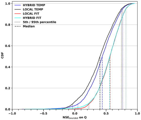
Figure 3 compares the performance of the hybrid model and the local, catchment-by-catchment linear regression in two settings: calibration (HYBRID FIT vs. LOCAL FIT) and temporal cross-validation (HYBRID TEMP vs. LOCAL TEMP). In the calibration setting, the cumulative distribution functions (CDFs) of HYBRID FIT and LOCAL FIT are almost indistinguishable, showing that the global, end-to-end training does not impose any noticeable constraint on in-sample performance compared to independent, catchment-by-catchment calibration. Under temporal cross-validation, by contrast, the HYBRID TEMP curve is clearly shifted toward higher NSEBOUNDED values compared to LOCAL TEMP, indicating that the globally trained hybrid model achieves better temporal robustness of the parameters than the locally calibrated regressions.

Figure 3Cumulative distribution functions of the NSEBOUNDED metric across the 3044 catchments for four models: the hybrid model under temporal cross-validation (HYBRID TEMP, blue), the local regression under temporal cross-validation (LOCAL TEMP, gray), and the hybrid model and local regression in calibration setting (HYBRID FIT, light blue, and LOCAL FIT, red). For HYBRID TEMP and LOCAL TEMP, the scores are computed on the testing periods.
Figure 4 presents the distributions of the inferred parameters for both approaches. For the local linear regressions, most coefficients related to evaporation () are set to zero because they are statistically nonsignificant; coefficients related to synchronicity () are also set to zero in many catchments. By contrast, the hybrid model produces parameter values that remain within the expected physical ranges of the three elasticity coefficients. It is worth noting that no bounds were imposed in this study: the neural network was free to produce any values, yet it nevertheless converged to physically coherent parameter sets. This behavior indicates that the hybrid approach can implicitly constrain the learned parameters toward interpretable and hydrologically consistent values while optimizing predictive performance. We note (Fig. 4 see the distributions of inferred parameters), that the potential evaporation and synchronicity elasticity coefficients are often statistically non-significant and set to zero in many catchments. We nevertheless retain these predictors for two reasons: where they are significant they add explanatory power at no structural cost (the coefficients are simply zeroed out otherwise); and, following Andréassian et al. (2025), the synchronicity term in particular captures a physically meaningful process (the temporal overlap between precipitation and potential evaporation) that can matter in specific climate contexts.

Figure 4Boxplots showing the distribution of the four model parameters across the 3044 catchments for the hybrid model under temporal cross-validation (HYBRID TEMP, blue), the local regression under temporal cross-validation (LOCAL TEMP, gray), and local regression in calibration setting (LOCAL FIT, red). For the elasticity coefficients, the shaded gray area indicates the expected physical range of parameter values (see Sect. 3.1). Boxes represent the 5th–95th percentile range across catchments, with the median indicated by the horizontal line inside each box.
4.2 Spatial transferability: difficulties in regionalizing the long-term streamflow mean
In a spatial cross-validation (regionalization) setting, performance drops substantially for both approaches relative to their training sets (Fig. 5). The loss of performance is larger in spatial cross-validation than in temporal cross-validation; spatiotemporal cross-validation shows a further, modest decrease relative to purely spatial cross-validation. This pattern indicates that the main difficulty for the annual model lies in spatial rather than temporal transfer.

Figure 5Cumulative distribution functions of the NSEBOUNDED metric across the 3044 catchments for the hybrid model under temporal cross-validation (HYBRID TEMP, blue), spatial cross-validation (HYBRID SPATIAL, green), and spatiotemporal cross-validation (HYBRID SPATIO-TEMP, magenta).
To identify the origin of the spatial performance loss, we analyzed the two components of the coupled model separately: (i) the annual anomaly (elasticity) model and (ii) the MQ estimation (the adjustment coefficient for the value given by the Turc–Mezentsev formula). Figure 6 shows the performance of the model on streamflow anomalies alone. The results indicate that the hybrid approach successfully regionalizes the anomaly model: the drop in performance between temporal and spatial cross-validation is minimal for anomalies. Therefore, the elasticity submodel (and its three coefficients) generalizes well across space.
Figure 7 reports the absolute relative error (ERA) between the predicted MQ and the observed MQ. While the MQ prediction error is small under temporal cross-validation (predicted MQ closely matches observed values), it increases markedly under spatial cross-validation. This observation suggests that the loss of performance in annual streamflow regionalization is primarily due to the model's inability to accurately predict MQ from the catchment descriptors. In short, the hybrid model can regionalize anomaly behavior well, but it struggles to derive spatially transferable relationships between descriptors and the parameters controlling MQ.

Figure 6Cumulative distribution functions of the NSEBOUNDED metric computed on the predicted streamflow anomaly ΔQ across the 3044 catchments for the hybrid model under temporal cross-validation (HYBRID TEMP, blue), spatial cross-validation (HYBRID SPATIAL, green), and spatiotemporal cross-validation (HYBRID SPATIO-TEMP, magenta).

Figure 7Boxplots of the absolute relative error on predicted interannual streamflow mean (ERA on MQ) across the 3044 catchments for the hybrid model under temporal cross-validation (HYBRID TEMP, blue), spatial cross-validation (HYBRID SPATIAL, green), and spatiotemporal cross-validation (HYBRID SPATIO-TEMP, magenta). For each model, two boxplots are displayed side by side: the training set (hatched box) and the test set (plain box). Boxes represent the 5th–95th percentile range across catchments, with the median indicated by the horizontal line inside each box.
5.1 Ability of the hybrid model to exploit information contained in the descriptors
To test whether the hybrid model actually exploits the physical information contained in the descriptors, we performed a control experiment inspired by the work of Li et al. (2022). In their study, they showed that for a global LSTM streamflow model, replacing physically based catchment descriptors with high-dimensional random vectors can still yield robust regionalization performance in gauged basins. Their results suggest that, in some settings, the deep learning model uses these vectors primarily as identifiers of individual catchments (rather than relying on their explicit physical meaning).
We adapted this idea to our hybrid modeling framework. Specifically, we constructed a “random-descriptor” setting in which, instead of using the real, physically based catchment descriptors, each catchment is assigned a random vector whose components are drawn independently from a standard normal distribution. In this setting, the descriptor vectors contain no physically interpretable information and do not preserve any geographical or climatic proximity among catchments. Comparing the performance and learned parameters obtained with these random descriptors against those obtained with the actual physical descriptors allows us to assess to what extent the hybrid model truly uses the physical content of the descriptors and whether its behavior resembles that observed by Li et al. (2022) for LSTM models or instead reflects a different dependence on descriptor information. The results of this experiment are shown in Fig. 8.
In temporal cross-validation, substituting real descriptors with random vectors causes only a small decrease in overall performance. The CDFs show that the largest degradation occurs in poorly predicted catchments (NSEBOUNDED< 0.3). For the better predicted catchments, performance is similar with real or random descriptors. This suggests that, in a temporal cross-validation setting, the network can use descriptors primarily as identifiers to distinguish catchments from one another (i.e., to locate a catchment in descriptor space), enabling the model to recover catchment-specific behavior during testing even when descriptors lack explicit physical information. This behavior is consistent with the findings of Li et al. (2022), who showed that a global LSTM can achieve nearly equivalent performance when physical descriptors are replaced by random vectors in a gauged prediction setting.
In spatial cross-validation, however, the difference between real and random descriptors is large and pronounced: using random descriptors yields substantially worse performance overall. This demonstrates that, for regionalization, the hybrid model relies on the physical content of the descriptors and can use it to build spatially transferable parameter estimates. When descriptors are random, the model can at best learn a generic mean parameter set and cannot capture meaningful spatial patterns. Consequently, as shown in Fig. 9, parameter variability across catchments is greatly reduced under random descriptors compared to the real-descriptor case. In contrast to the LSTM results reported by Li et al. (2022), our hybrid model therefore appears to require physically meaningful descriptors to sustain regionalization performance.

Figure 8Comparison of the hybrid model performance using random descriptors versus physically based descriptors. Cumulative distribution functions of the NSEBOUNDED metric across the 3044 catchments are shown for temporal cross-validation (HYBRID TEMP), spatial cross-validation (HYBRID SPATIAL), and spatiotemporal cross-validation (HYBRID SPATIO-TEMP). For each experiment, solid lines correspond to models trained with physically based catchment descriptors, while dashed lines correspond to models trained with random descriptors.
Taken together, these experiments indicate that:
-
the hybrid model exploits descriptors differently depending on the cross-validation task: as identifiers in temporal cross-validation (where catchment identity can be effectively recognized) and as carriers of physical information in spatial cross-validation (where transfer depends on meaningful relationships between descriptors and parameters);
-
the hybrid architecture is capable of learning physically interpretable parameter variations from descriptors, but its spatial transfer performance is limited by the current ability to predict the MQ from those descriptors.
These conclusions are consistent with the results presented in Sect. 4.2 and highlight the main remaining challenge: improving the mapping between catchment descriptors and MQ-controlling parameters so that MQ regionalization becomes as effective as anomaly regionalization. At the same time, the contrast with the work of Li et al. (2022) suggests that the dependence on descriptors may differ substantially between purely data-driven sequence models and hybrid models that explicitly separate long-term water balance from anomaly dynamics.

Figure 9Boxplots showing the distribution of the four model parameters across the 3044 catchments using random versus physically based descriptors for the hybrid model under temporal cross-validation (HYBRID TEMP, blue), spatial cross-validation (HYBRID SPATIAL, green), and spatiotemporal cross-validation (HYBRID SPATIO-TEMP, magenta). For each model, plain boxes correspond to physically based descriptors, while hatched boxes correspond to random descriptors with the same dimensionality. For the elasticity coefficients, the shaded gray area indicates the expected physical range of parameter values (see Sect. 3.1). Boxes represent the 5th–95th percentile range across catchments, with the median indicated by the horizontal line inside each box.
5.2 Limitations and perspectives
A key limitation of the proposed annual hybrid framework lies in the regionalization of the long-term streamflow mean (MQ). Although the elasticity component governing streamflow anomalies transfers well across space and time, the MQ component remains difficult to predict from catchment descriptors alone in our current formulation, which includes only a single multiplicative correction factor applied to the Turc–Mezentsev estimate. This difficulty is consistent with earlier work on regionalizing the Turc–Mezentsev water balance formula. Using a large set of French catchments, Lebecherel et al. (2013) systematically compared different ways of introducing regional information into this formula (by correcting simulated discharge directly, adjusting the aridity index, or modifying the Turc–Mezentsev shape parameter) and showed that the choice of correction term is critical, with correction of the aridity index emerging as the most robust solution when all catchments types are considered together. Our current MQ parameterization is conceptually closest to the first option (a multiplicative correction applied directly to the simulated discharge), which may partly explain its limited regionalization performance.
Building on these results, future work should focus on improving the representation and regionalization of long-term water balance, for instance, by testing alternative Budyko-type formulations, exploring more flexible parameterizations of the Turc–Mezentsev curve (beyond a single global correction factor), or explicitly representing additional controls such as groundwater storage, snow processes, or human influences. In particular, an interesting avenue would be to regionalize parameters that directly affect the aridity index or the shape of the Turc–Mezentsev curve, rather than merely scaling MQ a posteriori. A complementary strategy would be to treat MQ as a distinct sub-problem, possibly with its own loss function or a multi-task learning setup, instead of coupling it with the anomaly model through a single scalar correction. Applying the same anomaly-based decomposition to a conceptual daily rainfall–runoff model would also be an interesting way to test whether the benefits observed here at the annual scale carry over to finer temporal resolutions.
The experiments with random descriptors also reveal an important limitation in the use of catchment attributes. They suggest that the hybrid architecture exploits descriptors in markedly different ways depending on the cross-validation task: as quasi-identifiers in temporal cross-validation and as genuine carriers of physical information in spatial cross-validation. This contrast with the behavior reported for purely data-driven sequence models by Li et al. (2022) warrants a more systematic exploration of the interplay between descriptor spaces and hybrid model structure. In particular, it would be useful to investigate alternative sets of attributes (including dynamic or remotely sensed variables) and to examine to what extent feature selection, dimensionality reduction, or embedding strategies can enhance the spatial transferability of both the anomaly and MQ components.
Another limitation stems from the deliberate focus on a simple annual anomaly model. This choice helped isolate key mechanisms and avoid over-parameterization, but it also precluded the explicit representation of many intra-annual processes. Extending the proposed framework to finer temporal scales (seasonal, monthly, or daily) would enable the inclusion of additional processes such as snow accumulation and melt, soil moisture dynamics, or vegetation phenology, and would test whether the regularizing role of the physical backbone persists as model complexity increases. Such extensions, however, would face more severe equifinality issues and higher sensitivity to data quality, reinforcing the need for careful model design and robust transferability tests in the spirit of Klemeš (1986).
Finally, the present work focused on single-objective calibration based on the mean squared error of annual streamflow. Future developments could explore multi-objective and constraint-aware formulations, for example, by jointly optimizing streamflow performance and adherence to physically plausible parameter ranges, water balance closure, or independently derived elasticities. Differentiable programming offers a natural framework for incorporating such additional objectives or soft constraints, which could further stabilize parameter estimates under cross-validation and facilitate physical interpretation. In addition, the proposed annual hybrid framework could be used as a diagnostic tool to assess the robustness and transferability of more complex models. Being parsimonious, interpretable, and computationally inexpensive, the model could serve as a baseline for benchmarking large-scale hydrological simulations, identifying regions or periods where added structural complexity genuinely improves cross-validation performance. In this sense, annual hybrid models may play a dual role: not only as practical tools for large-scale water resources assessments, but also as reference frameworks for understanding when and where sophisticated hydrological and machine learning architectures are truly needed.
In this study, we proposed and evaluated a hybrid hydrological model that couples the Turc–Mezentsev formulation for the annual water balance with a data-driven elasticity model for annual streamflow anomalies. The approach was assessed across a large set of catchments under three experimental settings: temporal cross-validation, spatial cross-validation (regionalization), and combined spatiotemporal cross-validation.
First, our results show that, for temporal cross-validation, the hybrid approach with end-to-end learning outperforms local, catchment-by-catchment calibration. Joint training across all catchments yields parameter sets that are more temporally robust and achieve higher NSEBOUNDED scores than local calibrations. At the same time, the inferred elasticity coefficients remain within plausible physical ranges, even though no explicit constraint was imposed during training. This indicates that the hybrid architecture can leverage information shared across catchments to learn parameter sets that are both predictive and hydrologically interpretable.
Second, the experiments reveal a clear limitation of the current approach under spatial cross-validation. While the elasticity component governing streamflow anomalies generalizes well spatially, the model struggles to regionalize MQ: prediction errors on MQ remain small under temporal cross-validation but increase substantially under spatial and spatiotemporal cross-validation. The loss of performance in regionalization is thus primarily attributable to the difficulty of learning spatially transferable relationships between catchment descriptors and the correction factor used to adjust the Turc–Mezentsev MQ estimate in our model.
Third, the random-descriptor experiments clarify the role of descriptors in the hybrid model. Under temporal cross-validation, replacing the physically based descriptors by random vectors only slightly degrades performance, suggesting that the network uses the descriptors mainly as identifiers to distinguish individual catchments from each other. By contrast, under spatial cross-validation, performance drops markedly with random descriptors, and the variability of inferred parameters collapses toward a nearly global mean. This demonstrates that for regionalization, the hybrid model exploits the physical information in the descriptors to construct spatially coherent parameter fields.
Overall, these findings lead to two main conclusions. On the positive side, the hybrid framework successfully combines physical consistency with data-driven flexibility: it learns interpretable elasticity parameters, improves temporal transferability relative to local calibration, and leverages descriptors to enable spatial transfer of anomaly behavior. On the negative side, MQ regionalization emerges as the main bottleneck, limiting the overall performance of the annual hybrid model in spatial and spatiotemporal cross-validation.
Table A1Climate indices used to characterize catchment hydroclimatic conditions


Table A3Soil, subsurface, lithological, and morphological descriptors.

The data sources are listed in Tables 1, A1, A2, and A3. All datasets used in this work are publicly available: the CAMELS datasets are accessible from their respective repositories, as referenced in Tables 1, A1, A2 and A3, and all catchment descriptors used to train the neural network are derived from the openly accessible global data products listed in Appendix A. The list of the 3044 catchments used in this study, with their country, dataset and gauge identifier, is provided in the Supplement, as a table and as a CSV file.
The supplement related to this article is available online at https://doi.org/10.5194/hess-30-7061-2026-supplement.
AD conceived the study, implemented the model and experimental framework, carried out all simulations and analyses, and prepared the manuscript. VA and FB contributed to the experimental design, assembled and harmonized the multi-country dataset, and provided critical feedback on the methodology. CP contributed to the design of the experimental protocol and participated in the analysis and interpretation of the results. All authors discussed the results, revised the manuscript, and contributed to the final version of the paper.
The contact author has declared that none of the authors has any competing interests.
Publisher's note: Copernicus Publications remains neutral with regard to jurisdictional claims made in the text, published maps, institutional affiliations, or any other geographical representation in this paper. The authors bear the ultimate responsibility for providing appropriate place names. Views expressed in the text are those of the authors and do not necessarily reflect the views of the publisher.
This work was performed using HPC resources from GENCI–IDRIS (grant nos. 2024-AD010115988 and 2025-AD010115988R1). The authors would like to thank Guilherme M. Guimarães and Gaëlle Tallec for making the hydrological datasets used in this paper available and Isabella Athanassiou for copyediting this paper. We also thank the editor Wouter Berghuijs, David Post and the anonymous referee for their comments, which helped to improve this paper. AI-assisted tools (GitHub Copilot) were used to support language editing during manuscript preparation.
This research was funded by the Agence Nationale de la Recherche (project DRHYM ANR-22-CE56-0007).
This paper was edited by Wouter Berghuijs and reviewed by David Post and one anonymous referee.
Acuña Espinoza, E., Loritz, R., Álvarez Chaves, M., Bäuerle, N., and Ehret, U.: To bucket or not to bucket? Analyzing the performance and interpretability of hybrid hydrological models with dynamic parameterization, Hydrol. Earth Syst. Sci., 28, 2705–2719, https://doi.org/10.5194/hess-28-2705-2024, 2024.
Addor, N., Newman, A. J., Mizukami, N., and Clark, M. P.: The CAMELS data set: catchment attributes and meteorology for large-sample studies, Hydrol. Earth Syst. Sci., 21, 5293–5313, https://doi.org/10.5194/hess-21-5293-2017, 2017.
Ali, G., Tetzlaff, D., Soulsby, C., McDonnell, J. J., and Capell, R.: A comparison of similarity indices for catchment classification using a cross-regional dataset, Adv. Water Res., 40, 11–22, https://doi.org/10.1016/j.advwatres.2012.01.008, 2012.
Andréassian, V., Perrin, C., Berthet, L., Le Moine, N., Lerat, J., Loumagne, C., Oudin, L., Mathevet, T., Ramos, M.-H., and Valéry, A.: HESS Opinions “Crash tests for a standardized evaluation of hydrological models”, Hydrol. Earth Syst. Sci., 13, 1757–1764, https://doi.org/10.5194/hess-13-1757-2009, 2009.
Andréassian, V., Bourgin, F., Oudin, L., Mathevet, T., Perrin, C., Lerat, J., Coron, L., and Berthet, L.: Seeking genericity in the selection of parameter sets: Impact on hydrological model efficiency, Water Resour. Res., 50, 8356–8366, https://doi.org/10.1002/2013WR014761, 2014.
Andréassian, V., Coron, L., Lerat, J., and Le Moine, N.: Climate elasticity of streamflow revisited – an elasticity index based on long-term hydrometeorological records, Hydrol. Earth Syst. Sci., 20, 4503–4524, https://doi.org/10.5194/hess-20-4503-2016, 2016.
Andréassian, V., Guimarães, G. M., de Lavenne, A., and Lerat, J.: Time shift between precipitation and evaporation has more impact on annual streamflow variability than the elasticity of potential evaporation, Hydrol. Earth Syst. Sci., 29, 5477–5491, https://doi.org/10.5194/hess-29-5477-2025, 2025.
Arnell, N. W.: A simple water balance model for the simulation of streamflow over a large geographic domain, J. Hydrol., 217, 314–335, https://doi.org/10.1016/S0022-1694(99)00023-2, 1999.
Bergström, S.: Development and application of a conceptual runoff model for Scandinavian catchments, SMHI Report RHO 7, Swedish Meteorological and Hydrological Institute (SMHI), Norrköping, Sweden, https://www.smhi.se/publikationer-fran-smhi/sok-publikationer/1976-08-19-development-and-application-of-a-conceptual-runoff-model-for-scandinavian-catchments (last access: 12 November 2026), 1976.
Beven, K.: A manifesto for the equifinality thesis, J. Hydrol., 320, 18–36, https://doi.org/10.1016/j.jhydrol.2005.07.007, 2006.
Blöschl, G., Bierkens, M. F. P., Chambel, A., Cudennec, C., Destouni, G., Fiori, A., Kirchner, J. W., McDonnell, J. J., Savenije, H. H. G., Sivapalan, M., Stumpp, C., Toth, E., Volpi, E., Carr, G., Lupton, C., Salinas, J., Széles, B., Viglione, A., Aksoy, H., Allen, S. T., Amin, A., Andréassian, V., Arheimer, B., Aryal, S. K., Baker, V., Bardsley, E., Barendrecht, M. H., Bartosova, A., Batelaan, O., Berghuijs, W. R., Beven, K., Blume, T., Bogaard, T., Borges de Amorim, P., Böttcher, M. E., Boulet, G., Breinl, K., Brilly, M., Brocca, L., Buytaert, W., Castellarin, A., Castelletti, A., Chen, X., Chen, Y., Chen, Y., Chifflard, P., Claps, P., Clark, M. P., Collins, A. L., Croke, B., Dathe, A., David, P. C., de Barros, F. P. J., de Rooij, G., Di Baldassarre, G., Driscoll, J. M., Duethmann, D., Dwivedi, R., Eris, E., Farmer, W. H., Feiccabrino, J., Ferguson, G., Ferrari, E., Ferraris, S., Fersch, B., Finger, D., Foglia, L., Fowler, K., Gartsman, B., Gascoin, S., Gaume, E., Gelfan, A., Geris, J., Gharari, S., Gleeson, T., Glendell, M., Gonzalez Bevacqua, A., González-Dugo, M. P., Grimaldi, S., Gupta, A. B., Guse, B., Han, D., Hannah, D., Harpold, A., Haun, S., Heal, K., Helfricht, K., Herrnegger, M., Hipsey, M., Hlaváčiková, H., Hohmann, C., Holko, L., Hopkinson, C., Hrachowitz, M., Illangasekare, T. H., Inam, A., Innocente, C., Istanbulluoglu, E., Jarihani, B., Kalantari, Z., Kalvans, A., Khanal, S., Khatami, S., Kiesel, J., Kirkby, M., Knoben, W., Kochanek, K., Kohnová, S., Kolechkina, A., Krause, S., Kreamer, D., Kreibich, H., Kunstmann, H., Lange, H., Liberato, M. L. R., Lindquist, E., Link, T., Liu, J., Loucks, D. P., Luce, C., Mahé, G., Makarieva, O., Malard, J., Mashtayeva, S., Maskey, S., Mas-Pla, J., Mavrova-Guirguinova, M., Mazzoleni, M., Mernild, S., Misstear, B. D., Montanari, A., Müller-Thomy, H., Nabizadeh, A., Nardi, F., Neale, C., Nesterova, N., Nurtaev, B., Odongo, V. O., Panda, S., Pande, S., Pang, Z., Papacharalampous, G., Perrin, C., Pfister, L., Pimentel, R., Polo, M. J., Post, D., Prieto Sierra, C., Ramos, M.-H., Renner, M., Reynolds, J. E., Ridolfi, E., Rigon, R., Riva, M., Robertson, D. E., Rosso, R., Roy, T., Sá, J. H. M., Salvadori, G., Sandells, M., Schaefli, B., Schumann, A., Scolobig, A., Seibert, J., Servat, E., Shafiei, M., Sharma, A., Sidibe, M., Sidle, R. C., Skaugen, T., Smith, H., Spiessl, S. M., Stein, L., Steinsland, I., Strasser, U., Su, B., Szolgay, J., Tarboton, D., Tauro, F., Thirel, G., Tian, F., Tong, R., Tussupova, K., Tyralis, H., Uijlenhoet, R., van Beek, R., van der Ent, R. J., van der Ploeg, M., Van Loon, A. F., van Meerveld, I., van Nooijen, R., van Oel, P. R., Vidal, J.-P., von Freyberg, J., Vorogushyn, S., Wachniew, P., Wade, A. J., Ward, P., Westerberg, I. K., White, C., Wood, E. F., Woods, R., Xu, Z., Yilmaz, K. K., and Zhang, Y.: Twenty-three unsolved problems in hydrology (UPH) – a community perspective, Hydrol. Sci. J., 64, 1141–1158, https://doi.org/10.1080/02626667.2019.1620507, 2019.
Budyko, M. I.: Evaporation under natural conditions, Israel Program for Scientific Translations, Jerusalem, https://catalog.hathitrust.org/Record/001485946 (last access: 12 November 2026), 1963.
Chiew, F. H. S.: Lumped Conceptual Rainfall-Runoff Models and Simple Water Balance Methods: Overview and Applications in Ungauged and Data Limited Regions, Geography Compass, 4, 206–225, https://doi.org/10.1111/j.1749-8198.2009.00318.x, 2010.
Coron, L., Andréassian, V., Perrin, C., Lerat, J., Vaze, J., Bourqui, M., and Hendrickx, F.: Crash testing hydrological models in contrasted climate conditions: An experiment on 216 Australian catchments, Water Resour. Res., 48, 2011WR011721, https://doi.org/10.1029/2011WR011721, 2012.
Coxon, G., Addor, N., Bloomfield, J. P., Freer, J., Fry, M., Hannaford, J., Howden, N. J. K., Lane, R., Lewis, M., Robinson, E. L., Wagener, T., and Woods, R.: CAMELS-GB: hydrometeorological time series and landscape attributes for 671 catchments in Great Britain, Earth Syst. Sci. Data, 12, 2459–2483, https://doi.org/10.5194/essd-12-2459-2020, 2020.
Delaigue, O., Guimarães, G. M., Brigode, P., Génot, B., Perrin, C., Soubeyroux, J.-M., Janet, B., Addor, N., and Andréassian, V.: CAMELS-FR dataset: a large-sample hydroclimatic dataset for France to explore hydrological diversity and support model benchmarking, Earth Syst. Sci. Data, 17, 1461–1479, https://doi.org/10.5194/essd-17-1461-2025, 2025.
de Lavenne, A., Andréassian, V., Thirel, G., Ramos, M.-H., and Perrin, C.: A Regularization Approach to Improve the Sequential Calibration of a Semidistributed Hydrological Model, Water Resour. Res., 55, 8821–8839, https://doi.org/10.1029/2018WR024266, 2019.
de Lavenne, A., Andréassian, V., Crochemore, L., Lindström, G., and Arheimer, B.: Quantifying multi-year hydrological memory with Catchment Forgetting Curves, Hydrol. Earth Syst. Sci., 26, 2715–2732, https://doi.org/10.5194/hess-26-2715-2022, 2022.
European Commission: Global Land Cover 2000 database, European Commission, Joint Research Centre [data set], https://forobs.jrc.ec.europa.eu/glc2000 (last access: 12 November 2026), 2003.
Feng, D., Liu, J., Lawson, K., and Shen, C.: Differentiable, Learnable, Regionalized Process-Based Models With Multiphysical Outputs can Approach State-Of-The-Art Hydrologic Prediction Accuracy, Water Resour. Res., 58, https://doi.org/10.1029/2022WR032404, 2022.
Feng, D., Beck, H., Lawson, K., and Shen, C.: The suitability of differentiable, physics-informed machine learning hydrologic models for ungauged regions and climate change impact assessment, Hydrol. Earth Syst. Sci., 27, 2357–2373, https://doi.org/10.5194/hess-27-2357-2023, 2023.
Fowler, K. J. A., Peel, M. C., Western, A. W., Zhang, L., and Peterson, T. J.: Simulating runoff under changing climatic conditions: Revisiting an apparent deficiency of conceptual rainfall-runoff models, Water Resour. Res., 52, 1820–1846, https://doi.org/10.1002/2015WR018068, 2016.
Fowler, K., Coxon, G., Freer, J., Peel, M., Wagener, T., Western, A., Woods, R., and Zhang, L.: Simulating Runoff Under Changing Climatic Conditions: A Framework for Model Improvement, Water Resour. Res., 54, 9812–9832, https://doi.org/10.1029/2018WR023989, 2018.
Fowler, K. J. A., Zhang, Z., and Hou, X.: CAMELS-AUS v2: updated hydrometeorological time series and landscape attributes for an enlarged set of catchments in Australia, Earth Syst. Sci. Data, 17, 4079–4095, https://doi.org/10.5194/essd-17-4079-2025, 2025.
Fu, B.: On the calculation of the evaporation from land surface, Scientia Atmospherica Sinica, 5, 23–31, https://doi.org/10.3878/j.issn.1006-9895.1981.01.03, 1981.
Gleeson, T.: GLobal HYdrogeology MaPS (GLHYMPS) of permeability and porosity, University of Victoria Research Data Collection [data set], https://doi.org/10.5683/SP2/DLGXYO, 2018.
Grigg, A. H. and Hughes, J. D.: Nonstationarity driven by multidecadal change in catchment groundwater storage: A test of modifications to a common rainfall–run-off model, Hydrol. Proc., 32, 3675–3688, https://doi.org/10.1002/hyp.13282, 2018.
Hartmann, J. and Moosdorf, N.: The new global lithological map database GLiM: A representation of rock properties at the Earth surface, Geochem. Geophys. Geosyst., 13, 2012GC004370, https://doi.org/10.1029/2012GC004370, 2012.
Heng, S. and Suetsugi, T.: Comparison of regionalization approaches in parameterizing sediment rating curve in ungauged catchments for subsequent instantaneous sediment yield prediction, J. Hydrol., 512, 240–253, https://doi.org/10.1016/j.jhydrol.2014.03.003, 2014.
Höge, M., Scheidegger, A., Baity-Jesi, M., Albert, C., and Fenicia, F.: Improving hydrologic models for predictions and process understanding using neural ODEs, Hydrol. Earth Syst. Sci., 26, 5085–5102, https://doi.org/10.5194/hess-26-5085-2022, 2022.
Höge, M., Kauzlaric, M., Siber, R., Schönenberger, U., Horton, P., Schwanbeck, J., Floriancic, M. G., Viviroli, D., Wilhelm, S., Sikorska-Senoner, A. E., Addor, N., Brunner, M., Pool, S., Zappa, M., and Fenicia, F.: CAMELS-CH: hydro-meteorological time series and landscape attributes for 331 catchments in hydrologic Switzerland, Earth Syst. Sci. Data, 15, 5755–5784, https://doi.org/10.5194/essd-15-5755-2023, 2023.
Hrachowitz, M., Savenije, H. H. G., Blöschl, G., McDonnell, J. J., Sivapalan, M., Pomeroy, J. W., Arheimer, B., Blume, T., Clark, M. P., Ehret, U., Fenicia, F., Freer, J. E., Gelfan, A., Gupta, H. V., Hughes, D. A., Hut, R. W., Montanari, A., Pande, S., Tetzlaff, D., Troch, P. A., Uhlenbrook, S., Wagener, T., Winsemius, H. C., Woods, R. A., Zehe, E., and Cudennec, C.: A decade of Predictions in Ungauged Basins (PUB)– a review, Hydrol. Sci. J., 58, 1198–1255, https://doi.org/10.1080/02626667.2013.803183, 2013.
Huynh, N. N. T., Garambois, P., Colleoni, F., Renard, B., Roux, H., Demargne, J., Jay-Allemand, M., and Javelle, P.: Learning Regionalization Using Accurate Spatial Cost Gradients Within a Differentiable High-Resolution Hydrological Model: Application to the French Mediterranean Region, Water Resour. Res., 60, e2024WR037544, https://doi.org/10.1029/2024WR037544, 2024.
Jakeman, A. J. and Hornberger, G. M.: How much complexity is warranted in a rainfall-runoff model?, Water Resour. Res., 29, 2637–2649, https://doi.org/10.1029/93WR00877, 1993.
Jiang, S., Zheng, Y., and Solomatine, D.: Improving AI System Awareness of Geoscience Knowledge: Symbiotic Integration of Physical Approaches and Deep Learning, Geophys. Res. Lett., 47, https://doi.org/10.1029/2020GL088229, 2020.
Kim, U. and Kaluarachchi, J. J.: Application of parameter estimation and regionalization methodologies to ungauged basins of the Upper Blue Nile River Basin, Ethiopia, J. Hydrol., 362, 39–56, https://doi.org/10.1016/j.jhydrol.2008.08.016, 2008.
Kirchner, J. W.: Getting the right answers for the right reasons: Linking measurements, analyses, and models to advance the science of hydrology, Water Resour. Res., 42, 2005WR004362, https://doi.org/10.1029/2005WR004362, 2006.
Klemeš, V.: Operational testing of hydrological simulation models, Hydrol. Sci. J., 31, 13–24, https://doi.org/10.1080/02626668609491024, 1986.
Lan, T., Lin, K., Xu, C.-Y., Tan, X., and Chen, X.: Dynamics of hydrological-model parameters: mechanisms, problems and solutions, Hydrol. Earth Syst. Sci., 24, 1347–1366, https://doi.org/10.5194/hess-24-1347-2020, 2020.
Lebecherel, L., Andréassian, V., and Perrin, C.: On regionalizing the Turc-Mezentsev water balance formula, Water Resour. Res., 49, 7508–7517, https://doi.org/10.1002/2013WR013575, 2013.
Lebecherel, L., Andréassian, V., and Perrin, C.: On evaluating the robustness of spatial-proximity-based regionalization methods, J. Hydrol., 539, 196–203, https://doi.org/10.1016/j.jhydrol.2016.05.031, 2016.
Le Moine, N., Andréassian, V., Perrin, C., and Michel, C.: How can rainfall-runoff models handle intercatchment groundwater flows? Theoretical study based on 1040 French catchments, Water Resour. Res., 43, 2006WR005608, https://doi.org/10.1029/2006WR005608, 2007.
Li, X., Khandelwal, A., Jia, X., Cutler, K., Ghosh, R., Renganathan, A., Xu, S., Tayal, K., Nieber, J., Duffy, C., Steinbach, M., and Kumar, V.: Regionalization in a Global Hydrologic Deep Learning Model: From Physical Descriptors to Random Vectors, Water Resour. Res., 58, https://doi.org/10.1029/2021WR031794, 2022.
Liu, J., Koch, J., Stisen, S., Troldborg, L., Højberg, A. L., Thodsen, H., Hansen, M. F. T., and Schneider, R. J. M.: CAMELS-DK: hydrometeorological time series and landscape attributes for 3330 Danish catchments with streamflow observations from 304 gauged stations, Earth Syst. Sci. Data, 17, 1551–1572, https://doi.org/10.5194/essd-17-1551-2025, 2025.
Loritz, R., Dolich, A., Acuña Espinoza, E., Ebeling, P., Guse, B., Götte, J., Hassler, S. K., Hauffe, C., Heidbüchel, I., Kiesel, J., Mälicke, M., Müller-Thomy, H., Stölzle, M., and Tarasova, L.: CAMELS-DE: hydro-meteorological time series and attributes for 1582 catchments in Germany, Earth Syst. Sci. Data, 16, 5625–5642, https://doi.org/10.5194/essd-16-5625-2024, 2024.
Loshchilov, I. and Hutter, F.: Decoupled Weight Decay Regularization, in: International Conference on Learning Representations (ICLR 2019), https://openreview.net/forum?id=Bkg6RiCqY7 (last access: 12 November 2026), 2019.
Mathevet, T., Michel, C., Andréassian, V., and Perrin, C.: A bounded version of the Nash-Sutcliffe criterion for better model assessment on large sets of basins, in: Large Sample Basin Experiments for Hydrological Model Parameterization: Results of the Model Parameter Experiment – MOPEX, IAHS Publ. 307, 211–219, https://iahs.info/uploads/dms/13614.21--211-219-41-MATHEVET.pdf (last access: 12 November 2026), 2006.
McIntyre, N., Lee, H., Wheater, H., Young, A., and Wagener, T.: Ensemble predictions of runoff in ungauged catchments, Water Resour. Res., 41, 2005WR004289, https://doi.org/10.1029/2005WR004289, 2005.
Merz, R. and Blöschl, G.: Regionalisation of catchment model parameters, J. Hydrol., 287, 95–123, https://doi.org/10.1016/j.jhydrol.2003.09.028, 2004.
Merz, R., Parajka, J., and Blöschl, G.: Time stability of catchment model parameters: Implications for climate impact analyses, Water Resour. Res., 47, 2010WR009505, https://doi.org/10.1029/2010WR009505, 2011.
Mezentsev, V.: Back to the computation of total evaporation, Meteorologia i Gidrologia, 5, 24–26, 1955.
Montanari, A., Young, G., Savenije, H. H. G., Hughes, D., Wagener, T., Ren, L. L., Koutsoyiannis, D., Cudennec, C., Toth, E., Grimaldi, S., Blöschl, G., Sivapalan, M., Beven, K., Gupta, H., Hipsey, M., Schaefli, B., Arheimer, B., Boegh, E., Schymanski, S. J., Di Baldassarre, G., Yu, B., Hubert, P., Huang, Y., Schumann, A., Post, D. A., Srinivasan, V., Harman, C., Thompson, S., Rogger, M., Viglione, A., McMillan, H., Characklis, G., Pang, Z., and Belyaev, V.: “Panta Rhei – Everything Flows”: Change in hydrology and society – The IAHS Scientific Decade 2013–2022, Hydrol. Sci. J., 58, 1256–1275, https://doi.org/10.1080/02626667.2013.809088, 2013.
Muelchi, R., Rössler, O., Schwanbeck, J., Weingartner, R., and Martius, O.: An ensemble of daily simulated runoff data (1981–2099) under climate change conditions for 93 catchments in Switzerland (Hydro-CH2018-Runoff ensemble), Geosci. Data J., 9, 46–57, https://doi.org/10.1002/gdj3.117, 2022.
Nash, J. E. and Sutcliffe, J. V.: River flow forecasting through conceptual models part I – A discussion of principles, J. Hydrol., 10, 282–290, https://doi.org/10.1016/0022-1694(70)90255-6, 1970.
Oldekop, E.: Evaporation from the surface of river basins, Collection of the Works of Students of the Meteorological Observatory, University of Tartu-Jurjew-Dorpat, Tartu, Estonia, 209 pp., 1911.
Oudin, L., Hervieu, F., Michel, C., Perrin, C., Andréassian, V., Anctil, F., and Loumagne, C.: Which potential evapotranspiration input for a lumped rainfall–runoff model?, J. Hydrol., 303, 290–306, https://doi.org/10.1016/j.jhydrol.2004.08.026, 2005.
Oudin, L., Andréassian, V., Perrin, C., Michel, C., and Le Moine, N.: Spatial proximity, physical similarity, regression and ungaged catchments: A comparison of regionalization approaches based on 913 French catchments, Water Resour. Res., 44, 2007WR006240, https://doi.org/10.1029/2007WR006240, 2008.
Oudin, L., Kay, A., Andréassian, V., and Perrin, C.: Are seemingly physically similar catchments truly hydrologically similar?, Water Resour. Res., 46, 2009WR008887, https://doi.org/10.1029/2009WR008887, 2010.
Parajka, J., Merz, R., and Blöschl, G.: A comparison of regionalisation methods for catchment model parameters, Hydrol. Earth Syst. Sci., 9, 157–171, https://doi.org/10.5194/hess-9-157-2005, 2005.
Parajka, J., Viglione, A., Rogger, M., Salinas, J. L., Sivapalan, M., and Blöschl, G.: Comparative assessment of predictions in ungauged basins – Part 1: Runoff-hydrograph studies, Hydrol. Earth Syst. Sci., 17, 1783–1795, https://doi.org/10.5194/hess-17-1783-2013, 2013.
Paszke, A., Gross, S., Massa, F., Lerer, A., Bradbury, J., Chanan, G., Killeen, T., Lin, Z., Gimelshein, N., Antiga, L., Desmaison, A., Köpf, A., Yang, E., DeVito, Z., Raison, M., Tejani, A., Chilamkurthy, S., Steiner, B., Fang, L., Bai, J., and Chintala, S.: PyTorch: An Imperative Style, High-Performance Deep Learning Library, in: Advances in Neural Information Processing Systems 32 (NeurIPS 2019), https://proceedings.neurips.cc/paper_files/paper/2019/hash/bdbca288fee7f92f2bfa9f7012727740-Abstract.html (last access: 12 November 2026), 2019.
Pedregosa, F., Varoquaux, G., Gramfort, A., Michel, V., Thirion, B., Grisel, O., Blondel, M., Prettenhofer, P., Weiss, R., Dubourg, V., Vanderplas, J., Passos, A., Cournapeau, D., Brucher, M., Perrot, M., and Duchesnay, É.: Scikit-learn: Machine Learning in Python, J. Mach. Learn. Res., 12, 2825–2830, https://jmlr.org/papers/v12/pedregosa11a.html (last access: 12 November 2026), 2011.
Pelletier, J. D., Broxton, P. D., Hazenberg, P., Zeng, X., Troch, P. A., Niu, G., Williams, Z. C., Brunke, M. A., and Gochis, D.: Global 1-km Gridded Thickness of Soil, Regolith, and Sedimentary Deposit Layers, ORNL DAAC, Oak Ridge, Tennessee, USA [data set], https://doi.org/10.3334/ORNLDAAC/1304, 2016.
Perrin, C., Michel, C., and Andréassian, V.: Does a large number of parameters enhance model performance? Comparative assessment of common catchment model structures on 429 catchments, J. Hydrol., 242, 275–301, https://doi.org/10.1016/S0022-1694(00)00393-0, 2001.
Perrin, C., Michel, C., and Andréassian, V.: Improvement of a parsimonious model for streamflow simulation, J. Hydrol., 279, 275–289, https://doi.org/10.1016/S0022-1694(03)00225-7, 2003.
Perrin, C., Andréassian, V., Rojas Serna, C., Mathevet, T., and Le Moine, N.: Discrete parameterization of hydrological models: Evaluating the use of parameter sets libraries over 900 catchments, Water Resour. Res., 44, 2007WR006579, https://doi.org/10.1029/2007WR006579, 2008.
Poncelet, C.: Du bassin au paramètre: jusqu’où peut-on régionaliser un modèle hydrologique conceptuel?, PhD thesis, Université Pierre et Marie Curie, Paris, France, http://www.theses.fr/2016PA066550 (last access: 12 November 2026), 2016.
Razavi, T. and Coulibaly, P.: Streamflow Prediction in Ungauged Basins: Review of Regionalization Methods, J. Hydrol. Eng., 18, 958–975, https://doi.org/10.1061/(ASCE)HE.1943-5584.0000690, 2013.
Refsgaard, J. C. and Henriksen, H. J.: Modelling guidelines - terminology and guiding principles, Adv. Water Resour., 27, 71–82, https://doi.org/10.1016/j.advwatres.2003.08.006, 2004.
Reichstein, M., Camps-Valls, G., Stevens, B., Jung, M., Denzler, J., Carvalhais, N., and Prabhat: Deep learning and process understanding for data-driven Earth system science, Nature, 566, 195–204, https://doi.org/10.1038/s41586-019-0912-1, 2019.
Rojas-Serna, C., Lebecherel, L., Perrin, C., Andréassian, V., and Oudin, L.: How should a rainfall-runoff model be parameterized in an almost ungauged catchment? A methodology tested on 609 catchments, Water Resour. Res., 52, 4765–4784, https://doi.org/10.1002/2015WR018549, 2016.
Sankarasubramanian, A. and Vogel, R. M.: Annual hydroclimatology of the United States, Water Resour. Res., 38, https://doi.org/10.1029/2001WR000619, 2002.
Sankarasubramanian, A., Vogel, R. M., and Limbrunner, J. F.: Climate elasticity of streamflow in the United States, Water Resour. Res., 37, 1771–1781, https://doi.org/10.1029/2000WR900330, 2001.
Santos, L., Andréassian, V., Sonnenborg, T. O., Lindström, G., de Lavenne, A., Perrin, C., Collet, L., and Thirel, G.: Lack of robustness of hydrological models: a large-sample diagnosis and an attempt to identify hydrological and climatic drivers, Hydrol. Earth Syst. Sci., 29, 683–700, https://doi.org/10.5194/hess-29-683-2025, 2025.
Seibert, J.: Regionalisation of parameters for a conceptual rainfall-runoff model, Agricultural and Forest Meteorology, 98–99, 279–293, https://doi.org/10.1016/S0168-1923(99)00105-7, 1999.
Seibert, J.: Reliability of Model Predictions Outside Calibration Conditions, Hydrol. Res., 34, 477–492, https://doi.org/10.2166/nh.2003.0019, 2003.
Shen, C.: A Transdisciplinary Review of Deep Learning Research and Its Relevance for Water Resources Scientists, Water Resour. Res., 54, 8558–8593, https://doi.org/10.1029/2018WR022643, 2018.
Shen, C., Appling, A. P., Gentine, P., Bandai, T., Gupta, H., Tartakovsky, A., Baity-Jesi, M., Fenicia, F., Kifer, D., Li, L., Liu, X., Ren, W., Zheng, Y., Harman, C. J., Clark, M., Farthing, M., Feng, D., Kumar, P., Aboelyazeed, D., Rahmani, F., Song, Y., Beck, H. E., Bindas, T., Dwivedi, D., Fang, K., Höge, M., Rackauckas, C., Mohanty, B., Roy, T., Xu, C., and Lawson, K.: Differentiable modelling to unify machine learning and physical models for geosciences, Nat. Rev. Earth Environ., 4, 552–567, https://doi.org/10.1038/s43017-023-00450-9, 2023.
Siebert, S., Kummu, M., Porkka, M., Döll, P., Ramankutty, N., and Scanlon, B.: Historical Irrigation Dataset (HID), MyGeoHUB [data set], https://doi.org/10.13019/M20599, 2015.
Sivapalan, M., Takeuchi, K., Franks, S. W., Gupta, V. K., Karambiri, H., Lakshmi, V., Liang, X., McDonnell, J. J., Mendiondo, E. M., O'Connell, P. E., Oki, T., Pomeroy, J. W., Schertzer, D., Uhlenbrook, S., and Zehe, E.: IAHS Decade on Predictions in Ungauged Basins (PUB), 2003–2012: Shaping an exciting future for the hydrological sciences, Hydrol. Sci. J., 48, 857–880, https://doi.org/10.1623/hysj.48.6.857.51421, 2003.
Slater, L. J., Anderson, B., Buechel, M., Dadson, S., Han, S., Harrigan, S., Kelder, T., Kowal, K., Lees, T., Matthews, T., Murphy, C., and Wilby, R. L.: Nonstationary weather and water extremes: a review of methods for their detection, attribution, and management, Hydrol. Earth Syst. Sci., 25, 3897–3935, https://doi.org/10.5194/hess-25-3897-2021, 2021.
Stephens, C. M., Marshall, L. A., and Johnson, F. M.: Investigating strategies to improve hydrologic model performance in a changing climate, J. Hydrol., 579, 124219, https://doi.org/10.1016/j.jhydrol.2019.124219, 2019.
Thyer, M., Frost, A. J., and Kuczera, G.: Parameter estimation and model identification for stochastic models of annual hydrological data: Is the observed record long enough?, J. Hydrol., 330, 313–328, https://doi.org/10.1016/j.jhydrol.2006.03.029, 2006.
Tixeront, J.: Prévision des apports des cours d'eau, Publication de l'Association internationale d'hydrologie scientifique, 63, 118–126, 1964.
Tsai, W.-P., Feng, D., Pan, M., Beck, H., Lawson, K., Yang, Y., Liu, J., and Shen, C.: From calibration to parameter learning: Harnessing the scaling effects of big data in geoscientific modeling, Nat. Commun., 12, 5988, https://doi.org/10.1038/s41467-021-26107-z, 2021.
Turc, L.: Le bilan d'eau des sols : relations entre les précipitations, l'évaporation et l'écoulement, Annales agronomiques, 5, 491–595, 1954.
Vaze, J., Post, D. A., Chiew, F. H. S., Perraud, J.-M., Viney, N. R., and Teng, J.: Climate non-stationarity – Validity of calibrated rainfall–runoff models for use in climate change studies, J. Hydrol., 394, 447–457, https://doi.org/10.1016/j.jhydrol.2010.09.018, 2010.
Wolock, D. M., Winter, T. C., and McMahon, G.: Delineation and Evaluation of Hydrologic-Landscape Regions in the United States Using Geographic Information System Tools and Multivariate Statistical Analyses, Environ. Manag., 34, S71–S88, https://doi.org/10.1007/s00267-003-5077-9, 2004.