A physically integrated GNN surrogate for microbially-mediated kinetic reactive transport: PHYGNET

Reactive transport modelling (RTM) is essential for subsurface environmental management but is fundamentally constrained by traditional geochemical solvers. These solvers incur prohibitive computational costs and frequently suffer from numerical instabilities such as convergence failures, particularly in microbially-mediated kinetic reaction systems. While machine learning surrogates offer acceleration, they often lack physical consistency when dealing with stiff biogeochemical dynamics. Here we propose PHYGNET (Physically GNN Network), which maps microbial reaction networks into a directed graph by representing species and reactions as nodes and edges. It embeds Monod-type kinetics within a differentiable physics layer that enforces stoichiometric mass conservation and thermodynamic hierarchies, and incorporates a residual corrector that refines the final outputs at the cost of small deviations from exact mass balance. By successfully coupling with COMSOL, PHYGNET demonstrates the capability to execute full reactive transport simulations. Benchmark tests reveal that, in contrast to the severe super-linear time penalties faced by traditional solvers at engineering scales, PHYGNET maintains stable sub-linear scaling via tensor parallelism. At a scale of 10⁵ grid nodes, PHYGNET achieved an acceleration (up to 3588-fold) without numerical crashes. Furthermore, its escalating speedup ratio establishes a “small-sample training, ultra-large-scale inference” paradigm that effectively offsets initial data generation costs. Overall, PHYGNET provides an efficient and physically consistent framework for accelerating Monod-type microbial reactive transport simulations, offering a practical pathway for large-scale environmental applications.

1 Introduction

Reactive transport modelling (RTM) provides a process-based framework to quantitatively describe and predict the distribution of chemicals across spatial and temporal scales, while offering a rigorous means to test our understanding of the underlying processes and controlling factors (Meile and Scheibe, 2019; Steefel et al., 2015). Among these processes, microbially mediated reactions constitute a central driver of biogeochemical cycling, governing the transformation and redistribution of key elements under thermodynamically constrained conditions (Falkowski et al., 2008; Meile and Scheibe, 2019). To quantitatively resolve these dynamics, Monod-type kinetics, often implemented via Michaelis-Menten formulations, represent a widely adopted and foundational approach within the RTM framework (Johnson and Goody, 2011). These formulations explicitly capture substrate limitation, electron acceptor competition, and nonlinear transitions between metabolic regimes, enabling RTMs to reproduce complex redox zonation and pathway switching. Consequently, RTMs equipped with these biogeochemical modules have become indispensable not only for predictive applications, such as groundwater remediation (Brookfield et al., 2023; Prommer and Stuyfzand, 2005), but also for advancing mechanistic understanding of thermo-hydro-mechanical-chemical-biological (THMCB) coupling in geological systems (Mayer et al., 2002).

However, this mechanistic fidelity comes at a significant computational cost, as Monod-type formulations introduce strong nonlinearity and tight coupling among species. By expressing reaction rates as nonlinear functions of multiple substrates, electron acceptors, and environmental variables, these models generate highly coupled and stiff systems of ordinary differential equations. As a consequence, the geochemical reaction module becomes the primary computational bottleneck in RTMs (Laloy and Jacques, 2022; Silva et al., 2025), often requiring orders of magnitude more computational effort than transport calculations due to repeated nonlinear iterations and convergence control (De Lucia and Kühn, 2021; He et al., 2015). The computational cost of solving the geochemical reaction module escalates dramatically in large-scale or highly resolved simulations and is frequently accompanied by numerical instabilities, including convergence failures under extreme chemical gradients. (Deng et al., 2025). Such limitations severely restrict the feasibility of critical analyses (such as uncertainty quantification, parameter estimation, and inverse modelling), thereby hindering the broader application of RTMs in both scientific investigation and real-world decision-making (Fotherby et al., 2023; Shi et al., 2014). This fundamental trade-off between mechanistic fidelity and computational tractability remains a central challenge in modern reactive transport modelling.

This cost escalates further when reaction networks include sequential electron-acceptor pathways, such as aerobic respiration, denitrification, sulfate reduction, and methanogenesis, which introduce strong thermodynamic ordering, tight species coupling, and near-discontinuous redox transitions. Moreover, complex biogeochemical reaction networks can introduce numerical stiffness and convergence difficulties (Deng et al., 2025). These prohibitive computational expenses severely limit the feasibility of essential analyses, such as uncertainty quantification, parameter optimization, and inverse modelling, creating a significant barrier to their widespread use in decision-making and comprehensive system analysis (Fotherby et al., 2023; Shi et al., 2014).

In response to these challenges, researchers have increasingly turned to machine learning (ML) surrogates to accelerate RTMs (De Lucia and Kühn, 2021; Demirer et al., 2023; Jatnieks et al., 2016; Sprocati and Rolle, 2021). Parallel developments in groundwater science demonstrate the maturity of machine learning for subsurface prediction and inference, spanning groundwater-level forecasting (Kim et al., 2024; Solgi et al., 2021; Wu et al., 2025), contaminant source identification (Luo et al., 2025; Mo et al., 2019; Xu et al., 2025), and aquifer parameter inversion (Chen et al., 2025; Wang et al., 2025a; Zhan et al., 2023). However, surrogate modelling for complex biogeochemical kinetic reaction systems remains virtually unexplored. These reaction networks exhibit thermodynamically ordered pathways, sharp redox fronts, and tightly coupled pH-pe feedbacks, leading to stiff and highly nonlinear dynamics that conventional neural networks struggle to emulate (Koehn et al., 2021). Existing ML surrogates are generally black-box function approximators that do not enforce mass balance, inhibition effects, or reaction ordering (McGovern et al., 2019; Sturm and Wexler, 2022), causing error accumulation and instability during temporal rollout (Keller and Evans, 2019; Silva et al., 2025). This opaqueness undermines user trust and has prompted calls to develop inherently interpretable or physics-informed models instead of relying on completely opaque black-box approaches (Jiang et al., 2020; Rudin, 2019). As a result, despite progress in ML-accelerated hydrogeochemical modelling, there is still a lack of physically consistent and interpretable ML frameworks capable of handling full multi-pathway reaction networks.

To overcome these limitations, we turn to graph neural network (GNN). Nowadays, GNN have been extensively applied to molecular property prediction (Reiser et al., 2022), material screening (Zeng et al., 2022), catalysis modelling (Wang et al., 2025b), and has already proven its accuracy and practicality (Reiser et al., 2022; Midlagajni and Rothkopf, 2025). Since biogeochemical kinetic reactions inherently involve complex networks of chemical species and their interactions, these networks naturally resemble graph structures, where chemical species can be treated as nodes and reactions as edges or functional relationships. This structural analogy allows GNNs to inherently capture sequential, branched, and competitive reaction pathways. Moreover, GNNs offer architectural flexibility, they are not limited to fixed input shapes or predefined topologies, making them ideal for modelling systems with variable reaction networks. Studies have shown that trained GNNs generalize well across unseen graph structures or chemical mechanisms (Midlagajni and Rothkopf, 2025; Pang et al., 2024; Wu et al., 2025). Additionally, node and edge features in a GNN can directly encode domain knowledge (such as concentrations, reaction rates and environmental factors) making it possible to embed physical constraints and mechanistic understanding into the learning process. By explicitly embedding these physical mechanisms into the network architecture, GNNs provide a uniquely suited framework for the surrogate modelling of biogeochemical reaction systems.

Based on these considerations, we propose PHYGNET (Physically GNN Network), a physics-integrated GNN framework designed to accelerate microbially mediated kinetic reactive transport simulations while preserving mechanistic consistency. PHYGNET represents biogeochemical reaction systems as directed graphs, where chemical species and reaction pathways are encoded as graph components, and integrates a Monod-based kinetic physics layer to explicitly enforce stoichiometric constraints and mass conservation. A residual correction module is further incorporated to capture unresolved system-specific variations. To evaluate its applicability to complex reactive transport problems, PHYGNET is validated against representative multispecies biogeochemical kinetic systems, including thermodynamically ordered competitive degradation and sequential reductive dechlorination networks, and is further coupled with a COMSOL-based reactive transport framework for spatially distributed simulations. The performance of PHYGNET is systematically assessed in terms of predictive accuracy, long-term temporal stability during autoregressive simulations, physical consistency of the simulated geochemical states, and computational efficiency relative to conventional geochemical solvers. This study aims to establish a generalizable physics–ML framework for accelerating large-scale reactive transport modelling while retaining the fundamental chemical constraints required for reliable environmental predictions.

2 Methodology

The PHYGNET framework is developed as a modular architecture designed to emulate complex, microbially-mediated biogeochemical reaction networks. PHYGNET establishes a new mapping protocol that translates the stoichiometry and the kinetic logic of the given biogeochemical system into a physically integrated graph neural network. By leveraging the inherent structural analogy between biogeochemical pathways and directed graphs, the framework allows for the integration of reaction topologies, ranging from sequential electron-acceptor competition to complex, multi-species metabolic chains.

To demonstrate the framework's capabilities and validate its generalizability, this study utilizes two distinct and highly representative biogeochemical reaction networks: the thermodynamically ordered sequential degradation of toluene (a primary BTEX contaminant) and the chain reductive dechlorination of perchloroethylene (PCE). These systems encompass stiff nonlinearities, multi-electron-acceptor competition, and intricate inhibitory feedbacks among intermediate products (e.g., the well-documented “VC stall”). Evaluating the framework across the two networks suggests its potential applicability to other critical subsurface processes, such as microbially induced heavy metal reduction (e.g., U(VI) or Cr(VI) bioremediation) and nutrient cycling.

To rigorously test the limits of the PHYGNET framework, we move beyond simple porous media and apply it to a fractured aquifer system. The distinct flow channels and sharp gradients in fractured media (Hyman et al., 2017; Hyman and Jimenez-Martinez, 2018) provide a demanding environment for evaluating the model's stability and accuracy. In this section, we firstly introduce the numerical modelling of groundwater flow and solute transport. Next, we detail the mathematical formulations of the chemical reaction networks. Lastly, the components of PHYGNET will be introduced, including its detailed mathematical modelling and how it can be coupled with COMSOL to accomplish full reactive transport modelling (RTM).

2.1 Mathematical Modelling of Flow and Solute Transport in Fractured Media

The numerical simulation is conducted in a 2D rectangular domain measuring 0.5 m × 0.4 m. The domain represents a fractured porous medium where the rock matrix is treated as a continuum and fractures are explicitly represented using a Discrete Fracture Network (DFN) approach. We assume unsteady groundwater and solute transport in a pressurized, isotropic, fractured aquifer. We denote the 2D domain as Ω∈R² with the boundary Γ, in which the union of all fractures is denoted as Ω_f and the surrounding rock matrix as Ω_m. A conventional subscription “m” and “f” are adopted to denote the variables corresponding to the matrix and the fractures, respectively. Within Ω_m, the mass balance equation and the constitutive law are:

$$\begin{array}{}\text{(1)}& \begin{array}{rl}& {\displaystyle \frac{\partial }{\partial t}}\left({\mathit{ϵ}}_{\mathrm{p}}\mathit{\rho }\right)+\mathrm{\nabla }\cdot \left(\mathit{\rho }{q}_{\mathrm{m}}\right)=Q,\\ & q_{\mathrm{m}}=-{\displaystyle \frac{K_{\mathrm{m}}}{\mathit{\mu }}}\mathrm{\nabla }p,\end{array}\end{array}$$

Similarly, within the Ω_f

$$\begin{array}{}\text{(2)}& \begin{array}{rl}& d_{\mathrm{f}}{\displaystyle \frac{\partial }{\partial t}}\left({\mathit{ϵ}}_{\mathrm{p}}\mathit{\rho }\right)+{\mathrm{\nabla }}_{\mathrm{T}}\cdot \left(d_{\mathrm{f}}\mathit{\rho }{q}_{\mathrm{f}}\right)=d_{\mathrm{f}}Q,\\ & q_{\mathrm{f}}=-{\displaystyle \frac{K_{\mathrm{f}}}{\mathit{\mu }}}{\mathrm{\nabla }}_{\mathrm{T}}p,\end{array}\end{array}$$

where q_m and q_f are the Darcy flux in Ω_m and Ω_f respectively, p is the aqueous pressure, ϵ_p is the porosity, ρ is the density of water, Q is the external sources, d_f is the fracture aperture, K_m and K_f are the permeability of Ω_m and Ω_f respectively, within the Ω_f, ∇_T denotes the tangential direction along the fracture, indicating that the flow and pressure gradient are restricted to the one-dimensional fracture line within this two-dimensional model. K_f follows the cubic law.

For the solute transport model, we consider only advection and hydrodynamic dispersion, while the reaction term (S) which handled by the PHYGNET is solved separately. Thus, the governing equation of solute transport in Ω_m can be expressed as:

$$\begin{array}{}\text{(3)}& \begin{array}{rl}& {\displaystyle \frac{\partial {\mathit{ϵ}}_{\mathrm{p}}C}{\partial t}}+\mathrm{\nabla }\cdot J+q_{\mathrm{m}}\cdot \mathrm{\nabla }C=S,\\ & J=-D\mathrm{\nabla }C,\end{array}\end{array}$$

Similarly, within the Ω_f

$$\begin{array}{}\text{(4)}& \begin{array}{rl}& d_{\mathrm{f}}\left({\displaystyle \frac{\partial {\mathit{ϵ}}_{\mathrm{p}}C}{\partial t}}+{\mathrm{\nabla }}_{\mathrm{T}}\cdot J+q_{\mathrm{f}}\cdot {\mathrm{\nabla }}_{t}C\right)=d_{\mathrm{f}}S+n_{\mathrm{0}},\\ & J=-D{\mathrm{\nabla }}_{t}C,\end{array}\end{array}$$

where C is the concentration of solute, t demotes time, J is the hydrodynamic dispersion flux, S is the solute source/sink term, n₀ is initial solute amount in the fracture system, D is the hydrodynamic dispersion coefficient.

2.2 Mathematical Formulations of Kinetic Reaction Networks

In natural subsurface environments, microbially-driven biogeochemical transformations rarely occur as isolated, single-step processes. Instead, they manifest as complex, interconnected kinetic reaction networks. Whether modelling the thermodynamically ordered oxidation of hydrocarbons or the sequential reductive dechlorination of chlorinated solvents, the underlying mathematical architecture of these metabolic pathways shares a universal structure.

Consider a generalized biogeochemical reaction step j within a complex network, which can be conceptually represented by the following stoichiometry:

$$\begin{array}{}\text{(5)}& v_{A}A+v_{B}B\to v_{Y}Y+v_{Z}Z\end{array}$$

where A represents the primary substrate (i.e., a contaminant), B represents an electron acceptor or donor. Y and Z are the resulting products, and v the corresponding stoichiometric coefficients. r_j(C,E) is the kinetic rate of reaction j. This reaction rate is inherently a highly nonlinear function dependent on the concentration vector of all involved species (C) and the localized environmental state variables (E), such as pH, pe.

Mathematically, the temporal evolution of any chemical species i within a localized batch system (i.e., the reaction step in an operator-splitting RTM framework) is governed by a system of stiff, coupled ordinary differential equations (ODEs):

$$\begin{array}{}\text{(6)}& {\displaystyle \frac{\mathrm{d}{C}_i}{\mathrm{d}t}}=\sum _{j=\mathrm{1}}^M\pm {\mathit{\nu }}_{i,j}{r}_j(\mathbf{C},\mathbf{E})\end{array}$$

where C_i is the concentration of species i, t is the time, M is the total number of reactions in the network, v_i,j represents the stoichiometric coefficient of species i in reaction j (positive for products, negative for reactants).

The crux of the numerical complexity lies in the generalized kinetic rate, r_j. To capture the intricate biogeochemical dependencies, r_j is typically formulated as a multiplicative combination of a maximum rate capacity, substrate limitations, and inhibitory feedbacks among species. A generalized multi-Monod kinetic formulation can be expressed as:

$$\begin{array}{}\text{(7)}& r_j=k_{\max ,j}\cdot \left({\displaystyle \frac{C_A}{K_A+C_A}}\right)\cdot \left({\displaystyle \frac{C_B}{K_B+C_B}}\right)\cdot I_j\left(\mathbf{C}\right)\end{array}$$

where k_max,j is the maximum specific reaction rate (reflecting maximum specific microbial growth and biomass yield) under optimal environmental conditions (E). The fractional terms (e.g., $\frac{C_A}{K_A+C_A}$) are Monod expressions representing thermodynamic or enzymatic limitations, where K_i (e.g., K_A K_B) is the half-saturation constant of species i. These terms drive the reaction forward when substrates are abundant but choke it as concentrations approach zero. I_j(C) encapsulates the intricate inhibitory feedbacks from the surrounding chemical network.

In complex systems, the inhibition term I_j(C) acts as a regulatory gate. It is frequently modelled using competitive or non-competitive enzymatic inhibition functions, generalized as:

$$\begin{array}{}\text{(8)}& I_j\left(\mathbf{C}\right)=\prod _{x\in X_j}{\displaystyle \frac{K_{I,x}}{K_{I,x}+C_x}}\end{array}$$

where X_j is the set of all species that inhibit reaction j, C_x is the concentration of the inhibiting species x, and K_I,x is the inhibition threshold constant. This explicit mathematical term elegantly captures critical subsurface phenomena. For example, the presence of a thermodynamically more favourable electron acceptor (C_x) will suppress secondary metabolic pathways, or the accumulation of a toxic intermediate product will stall the downstream degradation chain.

The highly coupled nature of Eqs. (6) to (8), combined with feedback loops that can fluctuate over several orders of magnitude, results in severe numerical stiffness. Solving this generalized ODE system iteratively at every spatial grid cell using traditional Newton-Raphson methods imposes an overwhelming computational burden.

However, the inherent architecture of this generalized formulation exhibits a profound structural analogy to a directed graph. The discrete chemical species (A, B, Y, Z) serve as nodes, the stoichiometric transformations (v) form directed edges representing mass flow, and the inhibition terms (I_j) act as regulatory signals passed between specific nodes. This new topological mapping provides the foundational rationale for the PHYGNET framework, allowing the model to accelerate simulation efficiency by directly learning the message-passing dynamics of these structured biological networks.

2.3 Physically Integrated Surrogate GNN for Reactive Process

2.3.1 Framework Overview

Building upon the formal definition of the sequential kinetic pathways and their corresponding governing equations, we now proceed to the structural realization of the PHYGNET framework. By mapping the previously defined stoichiometry and inhibitory feedbacks into a directed graph topology, the model transitions from theoretical description to an active surrogate capable of emulating complex biogeochemical reaction-transport dynamics with high fidelity.

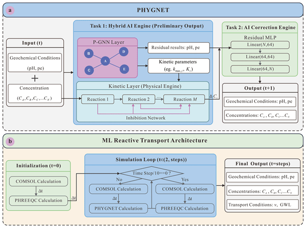
PHYGNET consists of three components: a parametric GNN (P-GNN), a Monod-based kinetic physics layer, and a residual corrector (see Fig. 1a). The P-GNN encodes each biogeochemical system as a directed graph, where nodes represent chemical species and reaction pathways, and edges capture reactant flows and inhibitory relationships. Node features include log-transformed concentrations. Through message passing, the P-GNN component learns latent embeddings (low-dimensional vector representations that encapsulate the topological and chemical context of each node) and uses them to predict biological kinetic parameters (i.e., k_max,j) for each pathway. These predicted parameters are then passed into the explicit kinetic physics layer, which deterministically calculates preliminary species concentrations, pH, and pe to ensure fundamental mass conservation and stoichiometric consistency. Finally, a lightweight multilayer perceptron (MLP) takes these preliminary physics-based results and outputs the final refined concentrations, pH, and pe by correcting residual errors, as this correction is not stoichiometrically constrained, the final outputs satisfy mass balance only approximately (quantified in Sect. 3.3). This decoupled architecture preserves interpretability while improving accuracy all target variables.

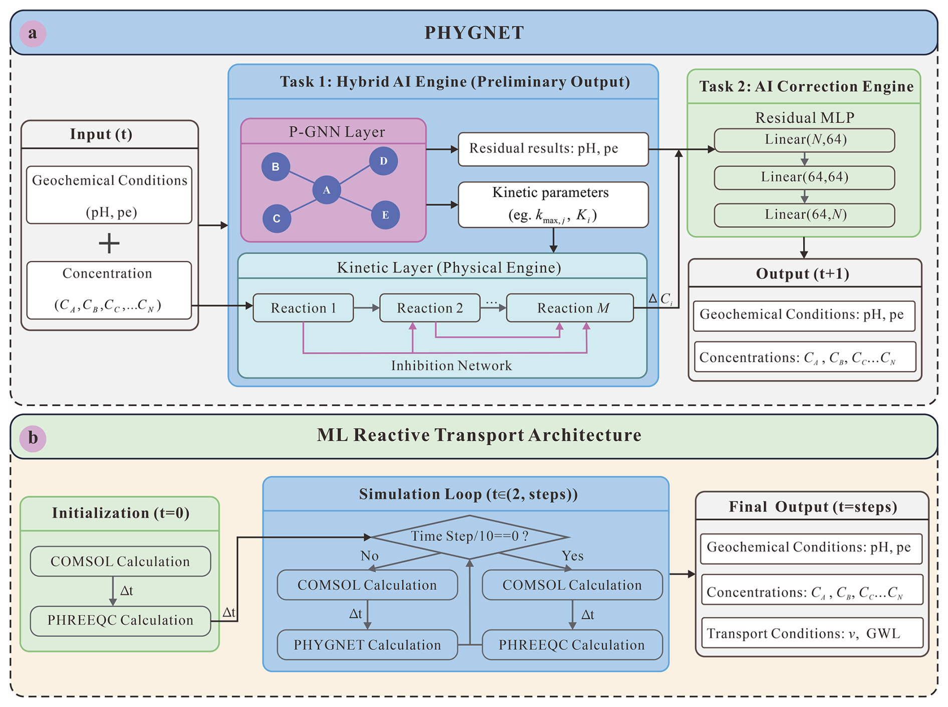
Figure 1 Overview of the PHYGNET framework and its integration into ML-accelerated RTMs. (a) PHYGNET combines a P-GNN for reaction kinetic parameter prediction, a Monod-based kinetic layer, and a residual MLP for correction. (b) In the ML RTM architecture, PHYGNET serves as a surrogate for PHREEQC between periodic recalibrations using the PHREEQC solver.

To seamlessly integrate physical consistency with predictive accuracy, PHYGNET adopts a multi-task learning strategy that simultaneously captures chemical dynamics and system states. Specifically, the model performs joint prediction of species concentrations, pH, pe, and the kinetic parameters, and this multi-task learning process is optimized during training through a unified loss function (detailed mathematically in Sect. 3.2.2, Eq. 18). This formulation enables shared latent representations that integrate fine-scale reactivity with global geochemical behaviour. In the PHYGNET architecture, predicted kinetic parameters function as learnable, physically plausible controls within Monod-type expressions. These parameters consistently align with traditional fixed values, demonstrating the model's capacity to infer reasonable ranges for unknown parameters. To investigate how PHYGNET infers latent kinetic parameters from sparse concentration fields without explicit supervision, we applied Shapley Additive Explanations (SHAP) analysis (Lundberg and Lee, 2017) to the predicted logarithmic rate constants (logk_max,i) and the residual correction terms. SHAP provides a theoretically grounded, game-theoretic attribution framework widely used to interpret machine-learning models in environmental and geoscience applications (Aldrees et al., 2025). The results are analysed in Sect. 4.4.

2.3.2 Detailed Mathematical Formulation of P-GNN

P-GNN is built on Graph Attention Network (GAT) layers. In a GAT layer each node's features are linearly transformed and then self-attention is used to weight contributions from neighbouring nodes. Specifically, for node i with feature vector h_i, we compute an attention score for each neighbour j∈N(i) as

$$\begin{array}{}\text{(9)}& e_{ij}=a^{\mathrm{T}}[W{\mathit{h}}_i\parallel W{\mathit{h}}_j]\end{array}$$

where W is a shared weight matrix, a is an attention vector, and “∥” denotes concatenation. These scores are normalized by a softmax over j to give attention coefficients.

$$\begin{array}{}\text{(10)}& {\mathit{\alpha }}_{ij}={\displaystyle \frac{\exp \left(e_{ij}\right)}{\sum _{k\in \mathcal{N}\left(i\right)}\exp \left(e_{ik}\right)}}\end{array}$$

The node's new feature is then a weighted sum of its neighbours:

$$\begin{array}{}\text{(11)}& {\mathit{h}}_i^{\prime }=\mathit{\sigma }\left(\sum _{j\in \mathcal{N}\left(i\right)}{\mathit{\alpha }}_{ij}W{\mathit{h}}_j\right)\end{array}$$

where σ is a nonlinearity (LeakyReLU). Multi-head attention is typically used: independent attention mechanisms compute features which are concatenated (or averaged in the final layer) to stabilize learning (Veličković et al., 2018). Here we use 4, 2, 1 in three GAT layers respectively.

To process this network, the P-GNN models the biogeochemical system as a graph comprising two distinct node types: chemical species nodes and reaction process nodes. As illustrated using the competitive degradation of HC (Fig. 2), directed edges connect these nodes to define their biogeochemical relationships. These connections are explicitly categorized into three edge types: reactant-to-reaction edges (solid black lines) indicating mass consumption, reaction-to-product edges (solid green lines) indicating mass generation, and inhibitory edges (dashed purple lines) representing regulatory signals (e.g., O₂ inhibiting sulfate reduction and methanogenesis).

Figure 2 Schematic of PHYGNET's reaction graph encoding in the P-GNN module.

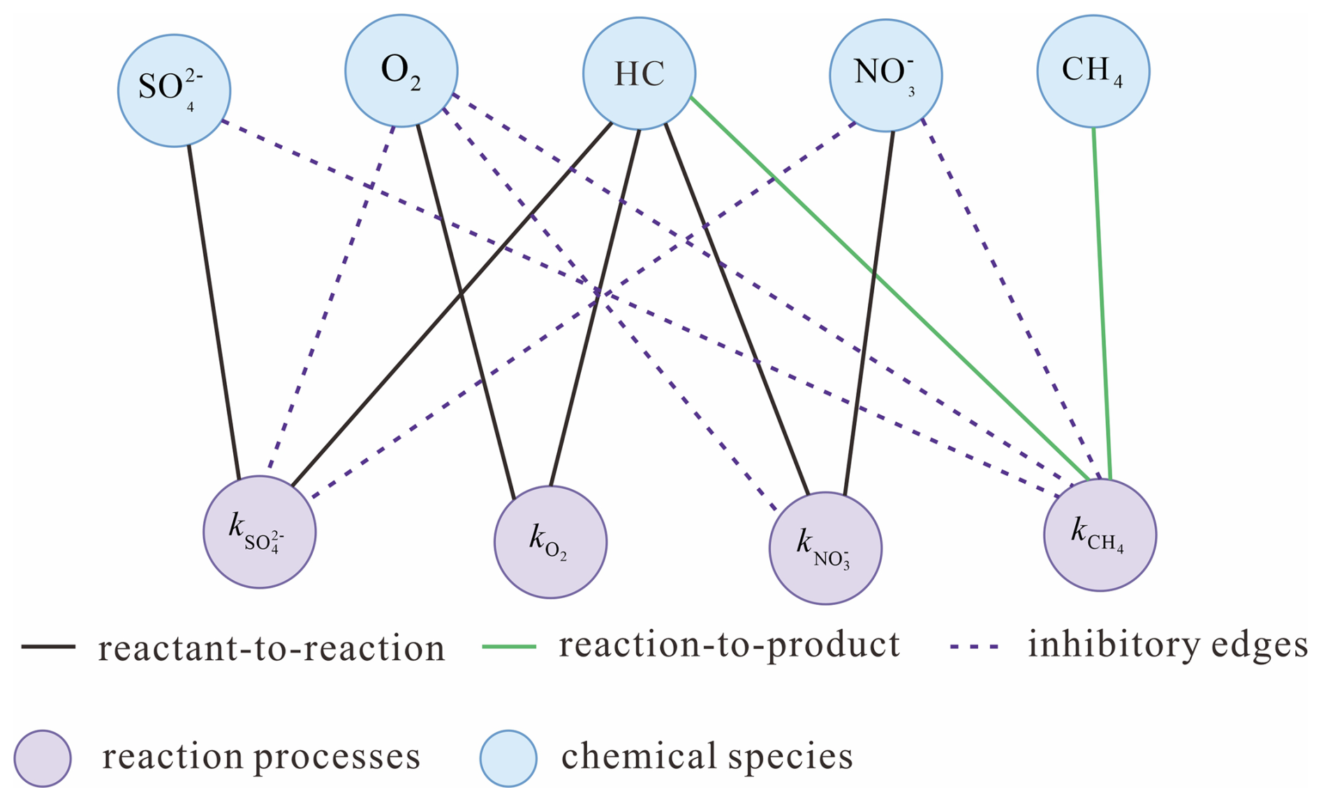
The P-GNN applies 3 stacked GAT layers to this specifically organized heterogeneous graph. At each layer, every individual node, whether representing a chemical species or a reaction process, receives messages from its incoming neighbours, weighted by the attention mechanism described above.

2.3.3 Integrating P-GNN with the Differentiable Kinetics Layer

While the P-GNN effectively captures the topological dependencies and predicts dynamic reaction constraints (e.g., k_max,j) based on message-passing algorithms, these purely data-driven outputs must be physically anchored. The core innovation of the framework lies in encoding the P-GNN within the broader PHYGNET architecture through a differentiable, hard-coded physics layer. This layer serves as a deterministic bridge between the abstract latent embeddings and the strict mass conservation laws governing hydrogeochemical systems.

Instead of allowing the neural network to directly predict future concentrations, PHYGNET restricts the P-GNN to predicting only the kinetic parameters. These predicted parameters are injected into the differentiable kinetics layer, which explicitly executes the multi-Monod rate laws and inhibition functions Eqs. (7) to (8), and enforces mass conservation within this layer through the stoichiometric matrix (v_i,j) defined within the governing ODE system (Eq. 6). By utilizing differentiable tensor operations, the layer calculates the exact mass of substrates consumed and intermediate products generated over the temporal step Δt.

This specific encoding strategy guarantees that, at the output of the differentiable kinetics layer and regardless of the specific biogeochemical reaction network being modelled, whether involving the parallel thermodynamic competition of electron acceptors (as seen in BTEX oxidation) or the sequential, inhibitory chain reactions of chlorinated solvents (such as PCE dechlorination), mass conservation is maintained. The generalized stoichiometric matrix (v_i,j) acts as an immutable physical inductive bias within the network.

Furthermore, real-world hydrogeochemical systems often exhibit subtle, unmodeled thermodynamic fluctuations. While the ground-truth target values for training are generated via comprehensive batch simulations using PHREEQC (detailed in Sect. 3.2.1), we deliberately avoid using a purely data-driven model to predict the final states directly, as such black-box models notoriously fail to maintain mass conservation in stiff kinetic systems. Instead, the physics-constrained concentration estimates are concatenated with the updated environmental features (E) and passed through a shallow Multi-Layer Perceptron (MLP) corrector. By restricting the MLP to learning only the residual differences between the physical approximations and the PHREEQC labels, this architecture keeps the final predicted state close to the mass-conserving physics-layer estimate while retaining the flexibility to capture complex environmental feedbacks. Because the residual correction is not itself stoichiometrically constrained, mass is conserved exactly only within the differentiable kinetics layer, and the final outputs satisfy mass balance approximately; the resulting deviations are quantified in Sect. 3.3.

Ultimately, this encoding paradigm ensures that during end-to-end training, the gradients computed from the final loss function flow backward through the immutable physics layer and into the P-GNN. This forces the graph network to continuously adjust its internal weights until it learns the true underlying biogeochemical dynamics, rather than merely memorizing statistical mappings.

2.4 Coupling PHYGNET with COMSOL

To demonstrate the surrogate model's capability in dynamic flow systems, we integrated PHYGNET into the CPqPy framework (see Fig. 1b). CPqPy originally couples COMSOL Multiphysics and PHREEQC through operator splitting, solving solute transport and reaction in alternating steps(Wei and Cao, 2022). We retained this architecture while substituting PHREEQC with PHYGNET for most time steps, and renamed it as CPgPy. Specifically, each time step begins with a solute transport simulation in COMSOL, from which nodal concentrations are extracted and passed to PHYGNET. These inputs (species concentrations, pH, and pe) are used to construct a batched reaction graph, which is then processed by PHYGNET to predict updated concentrations and environmental parameters. The predictions are converted back to COMSOL-readable formats and used to initialize the next transport step.

To prevent long-term drift and error accumulation, we adopt a hybrid strategy: every 10 simulation time steps, the framework calls PHREEQC to perform full geochemical simulation using the original kinetic definitions. This periodic correction stabilizes redox-sensitive parameters such as pH and pe, and helps recalibrate species interactions in the absence of explicit rate supervision. The input files for PHREEQC are automatically generated based on the latest COMSOL outputs and include both solution conditions and the defined reaction rates for each species, while the outputs are parsed back into the pipeline. This design ensures physical fidelity without sacrificing computational speed.

All modules are synchronized via a standardized file interface, ensuring compatibility with COMSOL's external input/output protocol. The entire system is controlled via Python, with MATLAB scripts used to initiate COMSOL simulations and restart services at each iteration for robustness. Through this integration, the PHYGNET-enabled CPgPy framework achieves efficient, modular simulation of reactive solute transport while preserving physical interpretability and model generalizability.

3 Application

To systematically evaluate the universal mapping capability and the physical fidelity of the PHYGNET framework, we establish two benchmark networks. These networks represent two of the most ubiquitous yet mathematically challenging biogeochemical kinetic systems in subsurface environments: thermodynamically ordered competitive oxidation (Case A) and sequential chain reductive dichlorination (Case B). By validating the surrogate against both systems, we ensure that PHYGNET's underlying topology mapping can accommodate fundamentally different biogeochemical architectures without structural modification.

3.1 Biogeochemical Kinetic Networks Setup

3.1.1 Case A: Competitive Degradation of BTEX

The first benchmark focuses on the aerobic and anaerobic oxidation of toluene (a representative BTEX compound), which involves multiple electron acceptors competing in a strict thermodynamic sequence. As groundwater transports the hydrocarbon plume, indigenous microbes preferentially utilize electron acceptors that yield the highest free energy. When dissolved oxygen O₂ is depleted, the system sequentially shifts to nitrate (NO${}_{\mathrm{3}}^{-}$), and subsequently to sulfate (SO${}_{\mathrm{4}}^{\mathrm{2}-}$), ultimately leading to methanogenesis.

This system is mathematically formulated using multiplicative Monod kinetics, incorporating competitive and non-competitive inhibitory functions to enforce the thermodynamic hierarchy. The reaction network is conceptualized as follows:

1. Aerobic Respiration.

   $$\begin{array}{}\text{(12)}& \begin{array}{rl}& {\mathrm{C}}_{\mathrm{7}}{\mathrm{H}}_{\mathrm{8}}+\mathrm{9}{\mathrm{O}}_{\mathrm{2}}+\mathrm{3}{\mathrm{H}}_{\mathrm{2}}\mathrm{O}\to \mathrm{7}\mathrm{HC}{\mathrm{O}}_{\mathrm{3}}^{-}+\mathrm{7}{\mathrm{H}}^{+}\\ & r_{{\mathrm{O}}_{\mathrm{2}}}=-k_{{\mathrm{O}}_{\mathrm{2}}}{C}_{\mathrm{HC}}{\displaystyle \frac{C_{{\mathrm{O}}_{\mathrm{2}}}}{K_{{\mathrm{O}}_{\mathrm{2}}}+C_{{\mathrm{O}}_{\mathrm{2}}}}}\end{array}\end{array}$$

2. Nitrate Reduction (Denitrification).

   $$\begin{array}{}\text{(13)}& \begin{array}{rl}& {\mathrm{C}}_{\mathrm{7}}{\mathrm{H}}_{\mathrm{8}}+\mathrm{7.2}{\mathrm{NO}}_{\mathrm{3}}^{-}+\mathrm{0.2}{\mathrm{H}}^{+}\to \mathrm{7}\mathrm{HC}{\mathrm{O}}_{\mathrm{3}}^{-}+\mathrm{3.6}{\mathrm{N}}_{\mathrm{2}}+\mathrm{0.6}{\mathrm{H}}_{\mathrm{2}}\mathrm{O}\\ & r_{\mathrm{N}{\mathrm{O}}_{\mathrm{3}}^{-}}=-k_{\mathrm{N}{\mathrm{O}}_{\mathrm{3}}^{-}}{C}_{\mathrm{HC}}{\displaystyle \frac{K_{\mathrm{inh},{\mathrm{O}}_{\mathrm{2}}}}{K_{\mathrm{I},{\mathrm{O}}_{\mathrm{2}}}+C_{{\mathrm{O}}_{\mathrm{2}}}}}{\displaystyle \frac{C_{\mathrm{N}{\mathrm{O}}_{\mathrm{3}}^{-}}}{K_{\mathrm{N}{\mathrm{O}}_{\mathrm{3}}^{-}}+C_{\mathrm{N}{\mathrm{O}}_{\mathrm{3}}^{-}}}}\end{array}\end{array}$$

3. Sulfate Reduction.

   $$\begin{array}{}\text{(14)}& \begin{array}{rl}& {\mathrm{C}}_{\mathrm{7}}{\mathrm{H}}_{\mathrm{8}}+\mathrm{4.5}{\mathrm{SO}}_{\mathrm{4}}^{\mathrm{2}-}+\mathrm{3}{\mathrm{H}}_{\mathrm{2}}\mathrm{O}+\mathrm{2}{\mathrm{H}}^{+}\to \mathrm{7}\mathrm{HC}{\mathrm{O}}_{\mathrm{3}}^{-}+\mathrm{4.5}{\mathrm{HS}}^{-}\\ & r_{{\mathrm{SO}}_{\mathrm{4}}^{\mathrm{2}-}}=-k_{{\mathrm{SO}}_{\mathrm{4}}^{\mathrm{2}-}}{C}_{\mathrm{HC}}{\displaystyle \frac{K_{I,{\mathrm{O}}_{\mathrm{2}}}}{K_{I,{\mathrm{O}}_{\mathrm{2}}}+C_{{\mathrm{O}}_{\mathrm{2}}}}}\\ & \cdot {\displaystyle \frac{K_{I,\mathrm{N}{\mathrm{O}}_{\mathrm{3}}^{-}}}{K_{I,\mathrm{N}{\mathrm{O}}_{\mathrm{3}}^{-}}+C_{\mathrm{N}{\mathrm{O}}_{\mathrm{3}}^{-}}}}{\displaystyle \frac{C_{{\mathrm{SO}}_{\mathrm{4}}^{\mathrm{2}-}}}{K_{{\mathrm{SO}}_{\mathrm{4}}^{\mathrm{2}-}}+C_{{\mathrm{SO}}_{\mathrm{4}}^{\mathrm{2}-}}}}\end{array}\end{array}$$

4. Methanogenesis.

   $$\begin{array}{}\text{(15)}& \begin{array}{rl}& {\mathrm{C}}_{\mathrm{7}}{\mathrm{H}}_{\mathrm{8}}+\mathrm{7.5}{\mathrm{H}}_{\mathrm{2}}\mathrm{O}\to \mathrm{2.5}\mathrm{HC}{\mathrm{O}}_{\mathrm{3}}^{-}+\mathrm{2.5}{\mathrm{H}}^{+}+\mathrm{4.5}{\mathrm{CH}}_{\mathrm{4}}\\ & r_{{\mathrm{CH}}_{\mathrm{4}}}=-k_{{\mathrm{CH}}_{\mathrm{4}}}{C}_{\mathrm{HC}}{\displaystyle \frac{K_{I,{\mathrm{O}}_{\mathrm{2}}}}{K_{I,{\mathrm{O}}_{\mathrm{2}}}+C_{{\mathrm{O}}_{\mathrm{2}}}}}\\ & \cdot {\displaystyle \frac{K_{I,\mathrm{N}{\mathrm{O}}_{\mathrm{3}}^{-}}}{K_{I,\mathrm{N}{\mathrm{O}}_{\mathrm{3}}^{-}}+C_{\mathrm{N}{\mathrm{O}}_{\mathrm{3}}^{-}}}}{\displaystyle \frac{K_{I,{\mathrm{SO}}_{\mathrm{4}}^{\mathrm{2}-}}}{K_{I,{\mathrm{SO}}_{\mathrm{4}}^{\mathrm{2}-}}+C_{{\mathrm{SO}}_{\mathrm{4}}^{\mathrm{2}-}}}}{\displaystyle \frac{C_{{\mathrm{CO}}_{\mathrm{2}}}}{K_{{\mathrm{CH}}_{\mathrm{4}}}+C_{{\mathrm{CO}}_{\mathrm{2}}}}}\end{array}\end{array}$$

The crucial numerical challenge here lies in the inhibition terms (e.g., $\frac{K_{I,{\mathrm{O}}_{\mathrm{2}}}}{K_{I,{\mathrm{O}}_{\mathrm{2}}}+C_{{\mathrm{O}}_{\mathrm{2}}}}$). These terms act as mathematical “switches” that suddenly activate or deactivate secondary reactions as the primary electron acceptor concentration approaches zero, creating sharp spatial and temporal gradients (stiffness) that are notoriously difficult for traditional solvers to integrate efficiently.

3.1.2 Case B: Sequential Reductive Dechlorination of PCE

To further test the framework's capability to capture chain reactions and intermediate product toxicity, we introduce the sequential reductive dechlorination of perchloroethylene (PCE) as the second benchmark. In highly reducing environments, specialized microbes (e.g., dehalococcoides) strip chlorine atoms from the solvent molecule, substituting them with hydrogen. The pathway proceeds stepwise from PCE to trichloroethylene (TCE), dichloroethylene (DCE), vinyl chloride (VC), and finally to benign Ethene, accompanied by the continuous release of chloride ions (Cl⁻).

Unlike the parallel competition in Case A, this system is characterized by sequential mass flow and profound cross-species inhibition. High concentrations of parent compounds (PCE and TCE) are known to strongly inhibit the degradation of downstream intermediates, a phenomenon that frequently leads to the dangerous accumulation of VC (a known carcinogen), often referred to as “VC stall”.

The mathematical formulation for this chain reaction utilizes multi-Monod kinetics with competitive inhibition terms. For instance, the degradation rate of DCE is suppressed by both PCE and TCE, while the degradation of VC is heavily suppressed by TCE and DCE. The generalized rate for a specific step (e.g., the degradation of component X to Y) is defined as:

$$\begin{array}{}\text{(16)}& \begin{array}{rl}& X\to Y+{\mathrm{Cl}}^{-}\\ & r_X=k_{\max ,X}\cdot \left({\displaystyle \frac{C_X}{K_X+C_X}}\right)\cdot \prod _{i\in P_X}\left({\displaystyle \frac{K_{I,i}}{K_{I,i}+C_i}}\right)\end{array}\end{array}$$

where P_X denotes the set of parent/inhibitory compounds affecting step X, and K_I,i is the competitive inhibition constant for compound i.

This specific kinetic structure forces the solver to track mass across multiple tightly coupled species. Even a minute error in predicting the early PCE dechlorination rate will exponentially propagate down the chain, completely distorting the predicted VC and Ethene concentrations. Therefore, this benchmark serves as an ultimate test for PHYGNET's differentiable physics layer, testing whether it can maintain mass-balance consistency across a multi-stage sequential pathway while correctly learning the complex interplay of downstream inhibitory signals.

3.2 Data Generation and Training Process

3.2.1 State Space Sampling and Ground Truth Simulation

To ensure the PHYGNET surrogate is robust and universally applicable across a highly heterogeneous macroscopic domain, the model must be trained on a comprehensive dataset that thoroughly explores the biogeochemical state space. Relying on a limited set of initial conditions often leads to severe out-of-distribution (OOD) errors when the surrogate encounters sharp concentration gradients or depleted zones during full reactive transport coupling. Therefore, we employed a systematic data generation and pre-processing pipeline applicable to both kinetic benchmarks.

We utilized Latin Hypercube Sampling (LHS) to efficiently sample the multi-dimensional parameter space, generating thousands of distinct initial state vectors (C₀, E₀). For Case A (BTEX), the sampled space included independent log-uniform distributions for HC, O₂, NO${}_{\mathrm{3}}^{-}$, SO${}_{\mathrm{4}}^{\mathrm{2}-}$, and CH₄, ensuring the model experiences scenarios ranging from fully aerobic to strictly methanogenic conditions. For Case B (PCE), The sampling space also explicitly covered a wide spectrum of parent (PCE, TCE) and daughter (DCE, VC, Ethene) product combinations. This deliberately included “bottleneck” scenarios (such as high PCE/TCE concentrations coexisting with trace VC) to compel the model to learn the critical “VC stall” inhibitory dynamics.

For each sampled initial state, a batch simulation was executed using the standard geochemical code PHREEQC. The solver was configured to strictly integrate the stiff ordinary differential equations defined in Section 3.1 over a designated simulation period. To mimic the discrete time-stepping inherent to the Operator-Splitting (OS) transport framework, the continuous concentration profiles were extracted at fixed intervals (Δt), producing paired input-output training tensors: $\mathit{\left\{}\right({\mathbf{C}}_t,{\mathbf{E}}_t)\to ({\mathbf{C}}_{t+\mathrm{\Delta }t},{\mathbf{E}}_{t+\mathrm{\Delta }t}\left)\mathit{\right\}}$. In total, about 50 000 discrete state transitions were generated for each benchmark system. Following data generation, the entire dataset was randomly partitioned to train and evaluate the model. Specifically, 80 % of the data was allocated to the training set, while the remaining 20 % was reserved as the testing set to validate model performance.

3.2.2 Data Transformation and Training Strategy

To map the tabular batch data into the graph-based format required by PHYGNET, the chemical species and reaction steps were encoded as node features within the topological structures defined in Fig. 1.

A critical pre-processing step in biogeochemical machine learning involves addressing the vast disparity in concentration scales. Chemical species concentrations can span more than ten orders of magnitude (e.g., from 10⁻³ mol L⁻¹ near a source zone to 10⁻¹² mol L⁻¹ at the plume fringe). Feeding raw linear concentrations into a neural network typically causes vanishing gradients for trace species. To mitigate this, all species concentrations were transformed using a regularized natural logarithm:

$$\begin{array}{}\text{(17)}& {C^{\prime }}_i={\displaystyle \frac{\ln \left(\max \right(C_i,\mathrm{0})+\mathit{ϵ})-{\mathit{\mu }}_i}{{\mathit{\sigma }}_i}}\end{array}$$

where ϵ is a conservatively small threshold (e.g., 10⁻¹² mol L⁻¹) representing the physical non-detect limit, and μ_i and σ_i are the mean and standard deviation of the log-transformed training set. Environmental state variables (pH, pe) were standardized using standard linear z-score normalization.

To strictly enforce the physics-informed inductive bias while allowing for minor thermodynamic flexibility, PHYGNET is trained end-to-end using a dual-task objective function. A single loss function targeting only the final output would allow the network to bypass physical laws; the P-GNN could potentially output absurdly large or unphysical maximum reaction rates, relying entirely on the MLP corrector to mathematically fit the data.

Task 1 (Physics Constraint). Evaluates the discrepancy between the purely physics-constrained predictions (output solely from the differentiable kinetics layer based on P-GNN's predicted k_max) and the ground truth.

Task 2 (Residual Correction). Evaluates the discrepancy of the final predictions after the residual MLP corrector has applied minor thermodynamic fine-tuning.

Because species concentrations in these successive reaction networks inherently span multiple orders of magnitude, a standard Mean Squared Error (MSE) loss suffers from severe numerical imbalance. The loss contributions are heavily dominated by high-concentration parent compounds, which disproportionately overshadows the errors associated with trace intermediate products. To compel the network to learn the intricate inhibitory dynamics of trace by-products (e.g., VC and Ethene), we employed a species-weighted Smooth L1 Loss (Huber Loss) function. The total loss L_total is formulated as:

$$\begin{array}{}\text{(18)}& \begin{array}{rl}{L}_{\mathrm{Task}}& =\sum _{i\in {\mathcal{V}}_{\mathrm{species}}}{\mathit{\omega }}_i\cdot \text{SmoothL1}({C^{\prime }}_{i,\mathrm{pred}},{C^{\prime }}_{i,\mathrm{true}})\\ & +\sum _{k\in \mathit{\left\{}\text{pH,pe}\mathit{\right\}}}\mathrm{SmoothL}\mathrm{1}(E_{k,\mathrm{pred}},E_{k,\mathrm{true}})\\ L_{\mathrm{total}}& =L_{\mathrm{Task}\mathrm{1}}+L_{\mathrm{Task}\mathrm{2}}\end{array}\end{array}$$

where ω_i is a manually assigned species-specific weight vector. Specifically, for the BTEX competitive system (Case A), the weight vector for [HC, O₂, NO${}_{\mathrm{3}}^{-}$, SO${}_{\mathrm{4}}^{\mathrm{2}-}$, CH₄] was set to [1.0, 1.0, 1.0, 1.0, 2.0]. For the sequential PCE dechlorination system (Case B), to strongly penalize “VC stall” mispredictions, the weight vector for [PCE, TCE, DCE, VC, Ethene] was scaled progressively as [1.0, 1.0, 2.0, 3.0, 3.0]. In our code implementation, higher weights were explicitly assigned to downstream daughter products to penalize sequential error propagation. Both tasks are optimized simultaneously, ensuring that the gradients flowing backward from L_Task1 strictly force the P-GNN to learn the true physical rate constants rather than relying entirely on the MLP corrector.

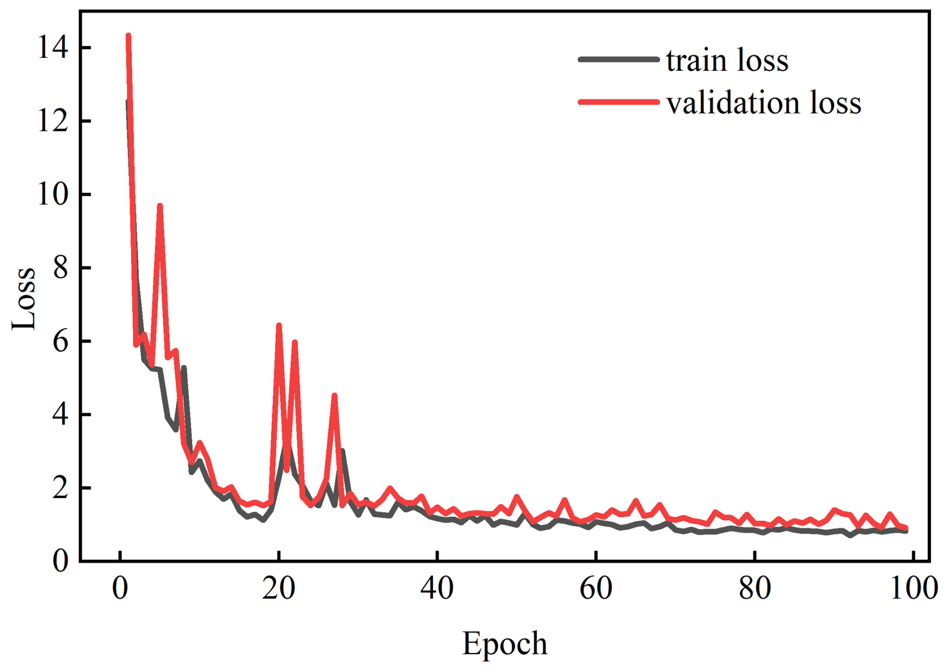
The framework was implemented using PyTorch Geometric and trained on an NVIDIA GPU using the Adam optimizer (initial learning rate of 10⁻³). An early stopping mechanism was deployed with a patience of 20 epochs to prevent overfitting. Figure 3 shows that the total loss and its components steadily decrease over training epochs, demonstrating both data fitting and physical regularization.

Figure 3 The total loss curves of training and validation (Case A).

To ensure the reproducibility of the computational performance, all simulations were executed on a standardized workstation equipped with an Intel Core i9-14900K CPU and an NVIDIA GeForce RTX 4090 GPU. The software environment was configured with COMSOL Multiphysics (v6.1), PyTorch (v2.4.1), and PHREEQC (v3.8.6).

During the model development phase, the PHYGNET was trained on the GPU using a batch size of 256. However, during the actual reactive transport simulations, the trained surrogate fully leveraged GPU acceleration to perform massively parallel predictions across all spatial grid nodes simultaneously. In contrast, the baseline physical simulations utilizing the PHREEQC engine were conducted in serial mode on the CPU. To represent a highly optimized traditional workflow, all independent reaction scenarios across the grid were compiled into a unified batch-input script, which was then solved sequentially without parallel multi-processing overhead.

3.3 Model Performance

To apply PHYGNET to RTMs, the first step should be to ensure that PHYGNET itself achieves sufficiently accurate simulation results. This high baseline accuracy is essential to minimize the propagation of surrogate-induced errors during the iterative spatial and temporal integration when coupled with the transport model. We evaluate the predictive performance of PHYGNET across two distinct kinetic networks: the competitive degradation of BTEX (Case A) and the sequential reductive dechlorination of PCE (Case B). The evaluation encompasses all output targets, including primary substrates, competing electron acceptors, intermediate daughter products, and geochemical conditions (pH, pe).

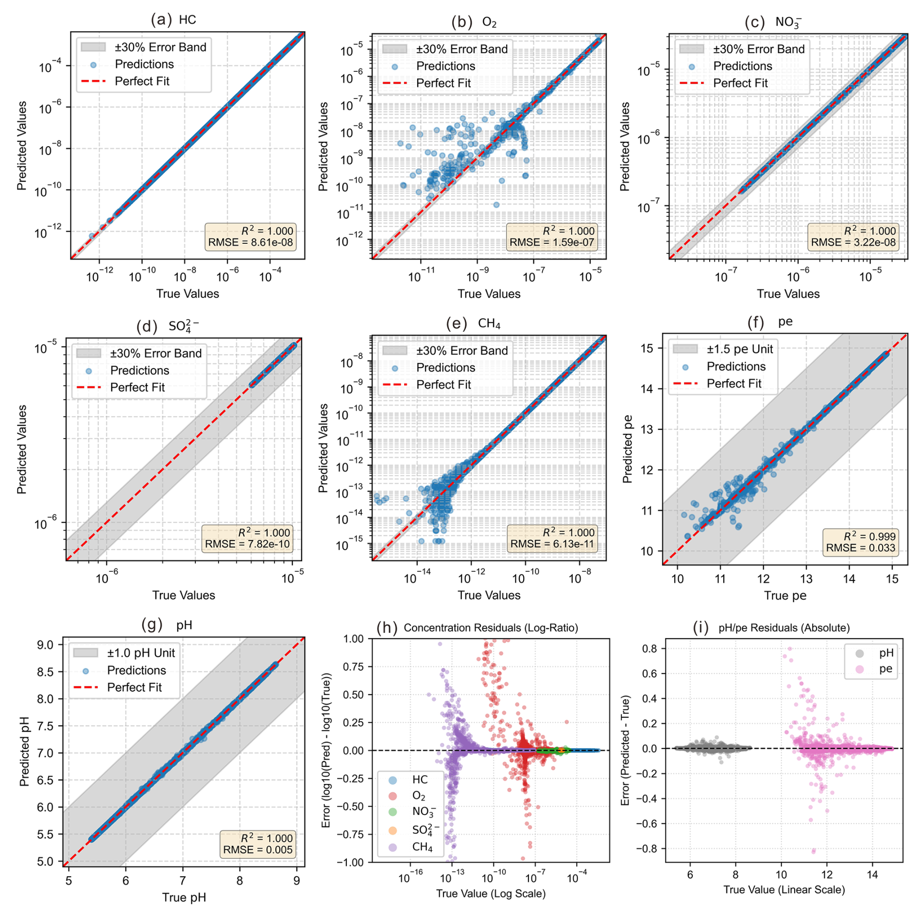
Figure 4 Predictive performance of PHYGNET for Case A. Scatter plots compare PHYGNET predictions and true values for five solute species (HC, O₂, NO${}_{\mathrm{3}}^{-}$, SO${}_{\mathrm{4}}^{\mathrm{2}-}$, CH₄) and two geochemical indicators (pH and pe). Lower-middle and lower-right panels show residual analysis for concentrations (log-ratio) and pH $/$ pe (absolute error).

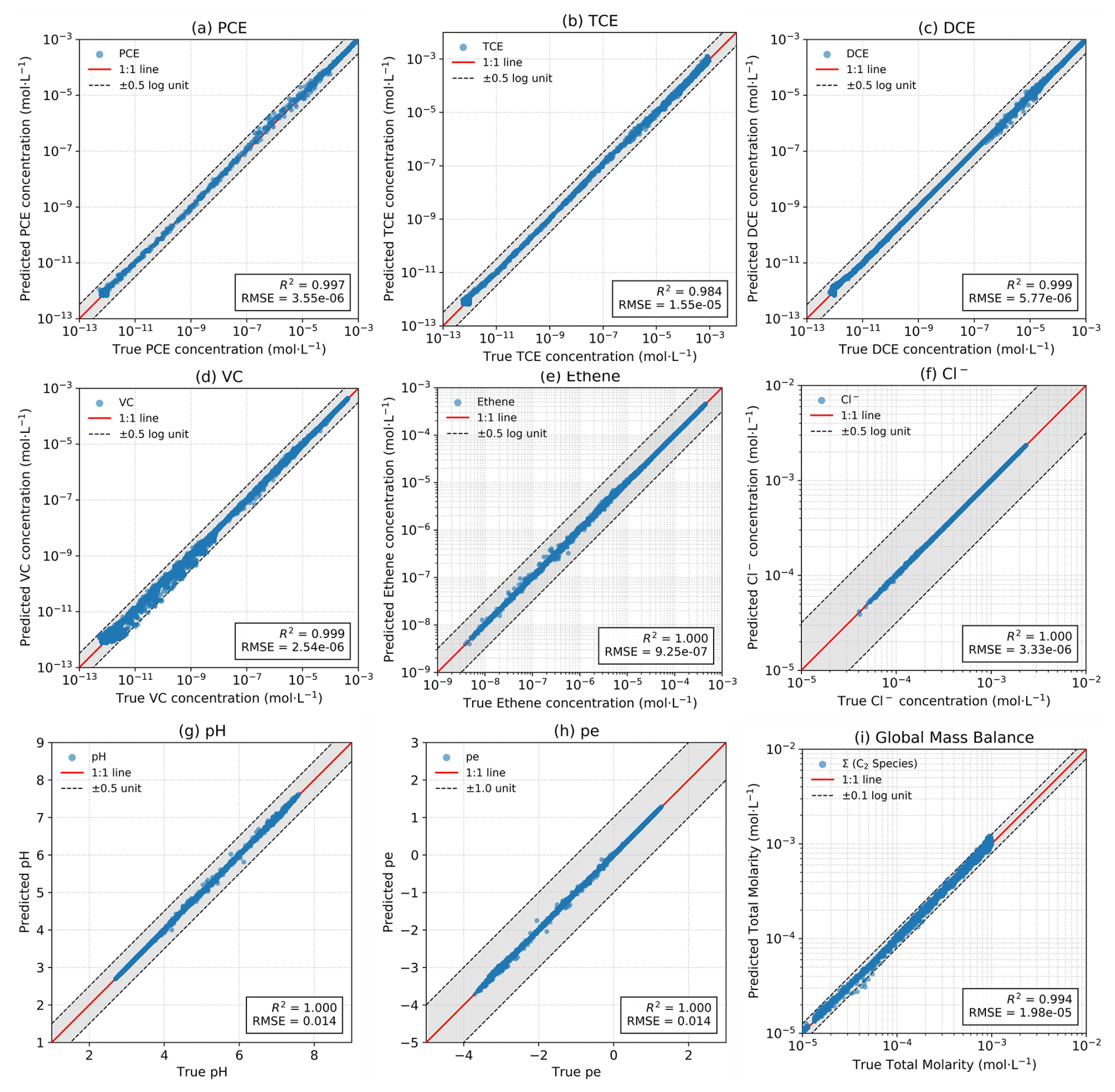
Figure 5 Predictive performance of PHYGNET for Case B. Panels (a)–(h) display the predictions for parent solvents, intermediate daughter products, and environmental variables. Panel (i) validates the global mass balance of C₂ backbone species (ΣPCE, TCE, DCE, VC, Ethene). The total molarity of the final PHYGNET outputs (after the MLP residual correction) closely follows the ground truth (R²=0.994, RMSE = $\mathrm{1.98}\times {\mathrm{10}}^{-\mathrm{5}}$ mol L⁻¹), with nearly all samples falling within the ± 0.1 log unit band, indicating that the mass-balance consistency provided by the internal physics layer is largely retained after residual correction.

Across all targets, PHYGNET achieves near-perfect agreement with ground truth values, reflected by R² scores above 0.98 and minimal root mean square errors (RMSE) (Fig. 4 for Case A; Fig. 5a–h for Case B). For the BTEX system (Case A), key species like HC and NO${}_{\mathrm{3}}^{-}$ exhibit near-zero deviation across all concentration regimes. Remarkably, the surrogate performs equally well in the PCE system (Case B), accurately capturing the complex, non-linear accumulation and decay dynamics of intermediate products like DCE and VC. The predictions for geochemical indicators (pH and pe) in both cases are also highly accurate, for instance, over 98 % of predictions fall well within ±0.5 pH units and ±1.0 pe units. These results validate PHYGNET's ability to simultaneously resolve fast-reacting organic species and slow-evolving redox environments while maintaining close mass-balance consistency.

To further probe the residual structure, we examined the log-ratio residuals for concentrations and absolute errors for pH $/$ pe. While the overall fidelity is exceptionally high, the largest relative uncertainties emerge predominantly in O₂ and CH₄ (for Case A), and trace levels of VC or Ethene (for Case B). These minor deviations stem from two primary physical and numerical causes:

1. Scale sensitivity at detection limits: These specific species often exist near physical non-detect limits (e.g., 10⁻¹⁵ to 10⁻¹⁰ mol L⁻¹). In this extreme low-concentration regime, even infinitesimally small absolute errors will translate into large log-scale variances on the parity plots.

2. Network hierarchy and error propagation: In Case A, the concentration of CH₄ is heavily influenced by upstream electron acceptors. The model must learn the implicit competition among O₂, NO${}_{\mathrm{3}}^{-}$, and SO${}_{\mathrm{4}}^{\mathrm{2}-}$. Similarly, in Case B, predicting trace VC and Ethene requires the model to correctly resolve the cascaded inhibitory feedbacks from PCE and TCE (the “VC stall” effect). These hierarchical dependencies introduce severe nonlinearities, making downstream trace species inherently more difficult to resolve perfectly than the primary substrates.

Despite these visible log-scale deviations at the lower bounds, the discrepancies are largely confined to extreme trace concentration levels approaching the numerical precision limits of the solver, where computational round-off and discretization effects naturally dominate (Hammond et al., 2014). Such errors are ubiquitous in traditional RTMs and are unlikely to affect macroscopic plume interpretation or transport simulation accuracy, as they fall well within the noise level of environmental measurement or numerical approximation (Li et al., 2008). Importantly, PHYGNET retains pristine fidelity across all ecologically and computationally relevant concentration ranges for both competitive and sequential reaction networks.

Crucially, while resolving trace-level intermediate products poses a significant challenge, the PHYGNET framework substantially mitigates a major weakness of traditional purely data-driven surrogates: the violation of mass conservation. As demonstrated in Fig. 5i, we evaluated the global mass balance of the Case B network by tracking the total molarity of all two-carbon (C2) species (Σ(PCE, TCE, DCE, VC, ethene)) over all 9900 validation transitions. Because the sequential dechlorination process merely strips chlorine atoms while leaving the C2 carbon backbone intact, the sum of these species must theoretically remain constant throughout the temporal integration. As Fig. 5i illustrates, the total molarities of the final outputs after residual correction follow the 1:1 ground truth line (R²=0.994, RMSE = $\mathrm{1.98}\times {\mathrm{10}}^{-\mathrm{5}}$ mol L⁻¹), with nearly all test samples falling within ±0.1 log units. To quantify this, we define the relative closure error of a single integration step as

$$\begin{array}{}\text{(19)}& \mathit{ϵ}={\displaystyle \frac{\mathrm{\Sigma }\text{C2}\left(t+\mathrm{\Delta }t\right)-\mathrm{\Sigma }\text{C2}\left(t\right)}{\mathrm{\Sigma }\text{C2}\left(t\right)}}\end{array}$$

For the final outputs after residual correction, the mean absolute closure error is $\mathrm{1.4}\times {\mathrm{10}}^{-\mathrm{2}}$ with an RMSE of $\mathrm{2.7}\times {\mathrm{10}}^{-\mathrm{2}}$, and 61.6 % of transitions close to better than 1 %. We regard a mean violation below 2 % as an acceptable cost for the accuracy the corrector recovers on the trace intermediates. The proposed architecture therefore represents a practical compromise between computational precision and physical fidelity.

4 Discussions

Having successfully validated the surrogate's high-fidelity emulation and topological generalizability at the batch scale, this section evaluates the PHYGNET framework's macroscopic utility and internal physical consistency.

The subsequent discussion evaluates PHYGNET across three key dimensions: macroscopic RTM performance (Sect. 4.1 and 4.2), computational efficiency (Sect. 4.3), and model interpretability (Sect. 4.4). Given that the operator-splitting interface is inherently system-agnostic, a single spatial demonstration is mathematically sufficient to validate the framework's robustness. Consequently, we focus on the BTEX competitive degradation system (Case A) embedded within a highly heterogeneous fractured aquifer. This scenario rigorously tests the surrogate's stability, spatial accuracy, and computational acceleration under extreme physical gradients. Furthermore, we apply SHAP (Shapley Additive Explanations) analysis to confirm that the network autonomously learns the underlying biogeochemical logic, capturing both competitive and sequential-inhibitory mechanisms, rather than simply overfitting the training data.

4.1 Setup of the Fractured Aquifer RTM

Specially, we simulate reactive transport within a 2D fractured domain using the CPgPy framework. Establishing validity in this highly heterogeneous condition suggests that the framework can readily extend to other subsurface conditions. The rectangular domain measures 0.5 m × 0.4 m and incorporates two intersecting fracture sets: three fractures oriented at 310° and three at 60°, respectively. A discrete fracture network (DFN) approach is adopted, with local mesh refinement along fracture planes to resolve sharp hydraulic and chemical gradients (see Fig. 6).

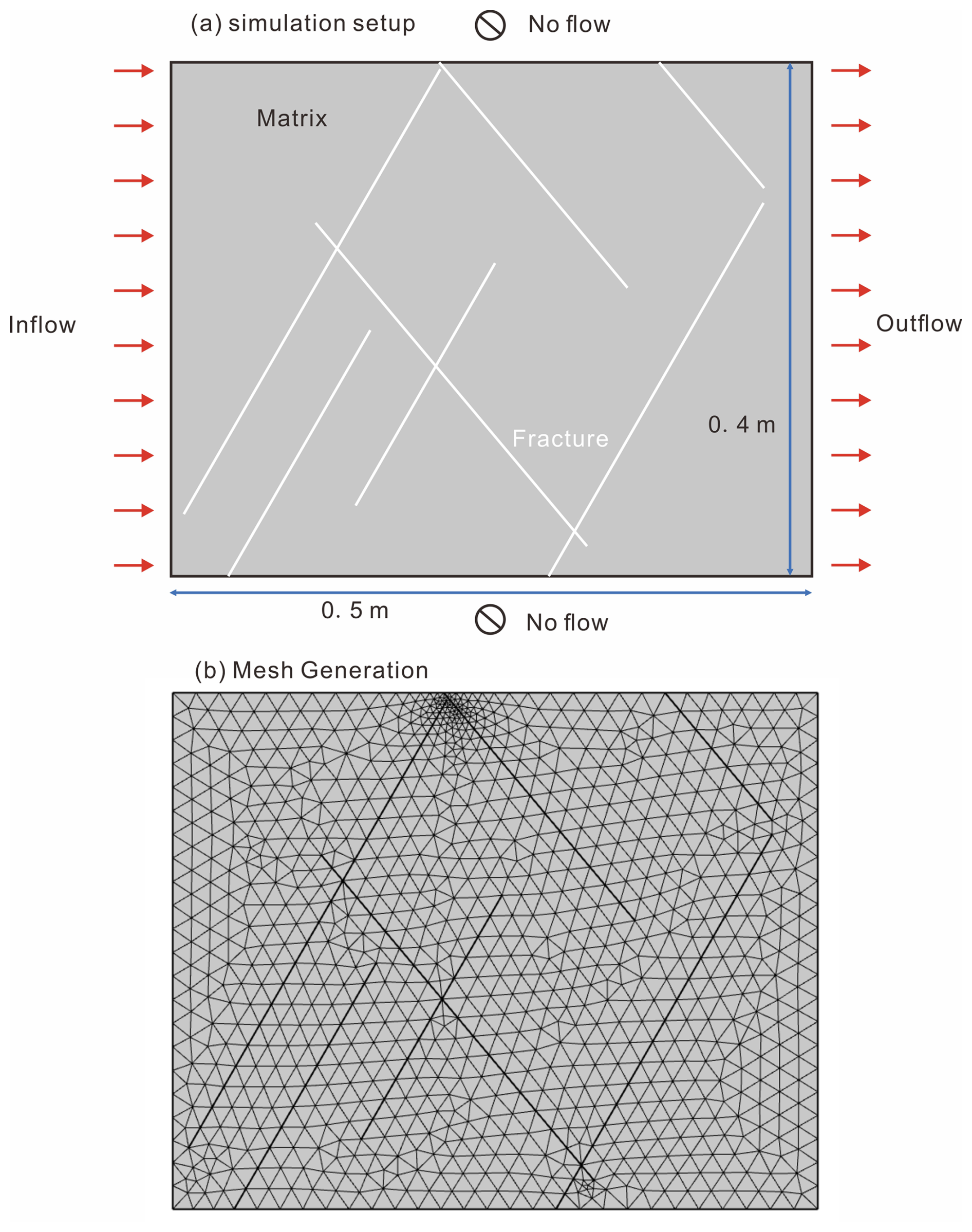
Figure 6 Schematic of the idealized 2D fractured aquifer domain and mesh generation. (a) Simulation setup: A 0.5 m × 0.4 m rectangular domain representing a porous matrix with embedded fractures. Red arrows indicate inflow from the left boundary and outflow from the right boundary; top and bottom boundaries are no-flow conditions. Fractures are depicted as white lines traversing the matrix. (b) Mesh Generation: Unstructured triangular mesh discretizing the domain, with finer resolution near fracture intersections to capture localized gradients in concentration or velocity. Mesh aligns with fracture geometry to ensure accurate representation of flow and reaction processes.

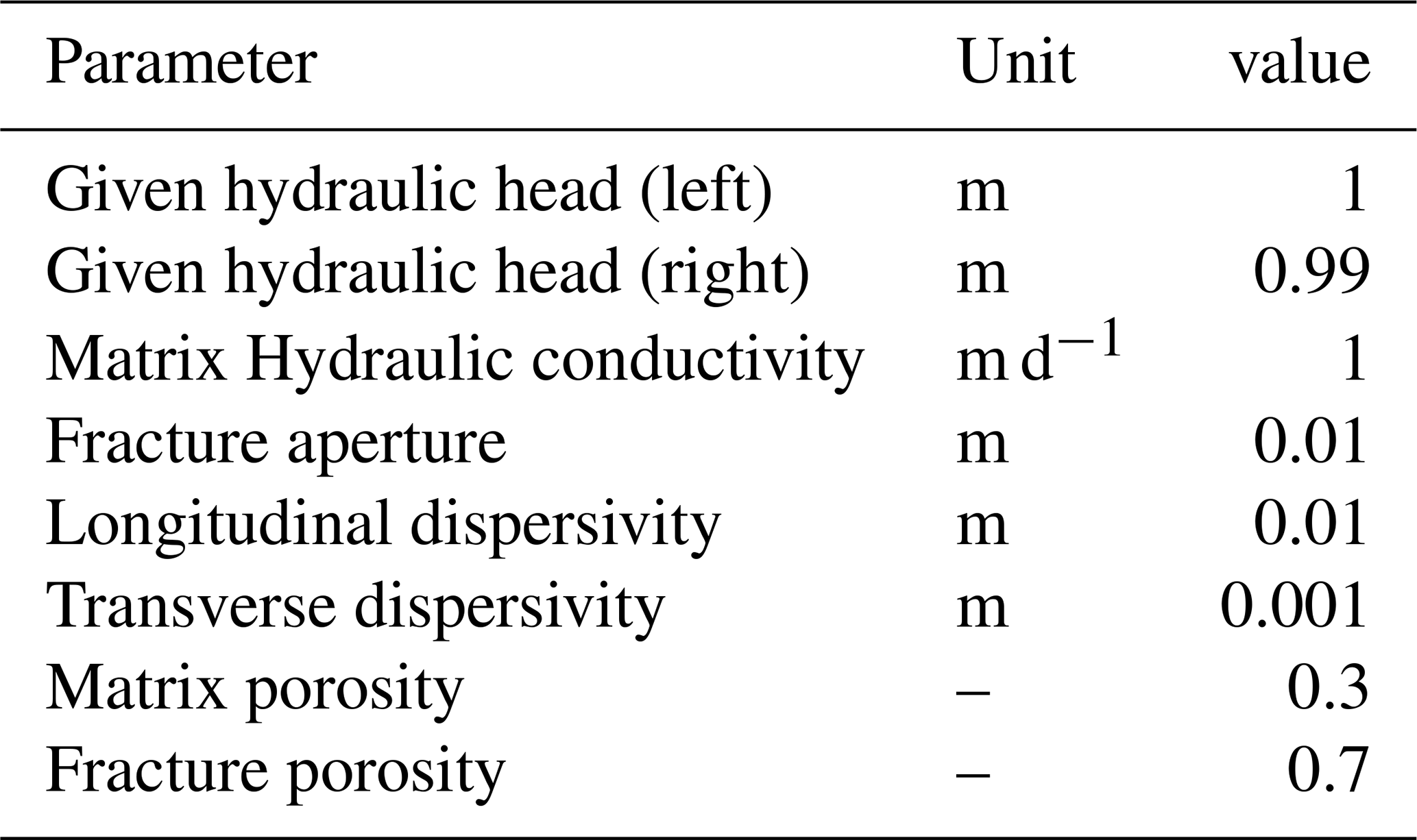
Groundwater flow is driven by given-head boundaries on the left and right edges, establishing a horizontal hydraulic gradient of 0.02 from left to right. The top and bottom boundaries are treated as no-flow. Solute transport is solved with the advection-dispersion equation, with flow field solved with a groundwater flow model built into COMSOL. The mesh is generated with refinement around fractures to capture the sharp velocity and concentration gradients at the fracture-matrix interfaces (see Fig. 6b).

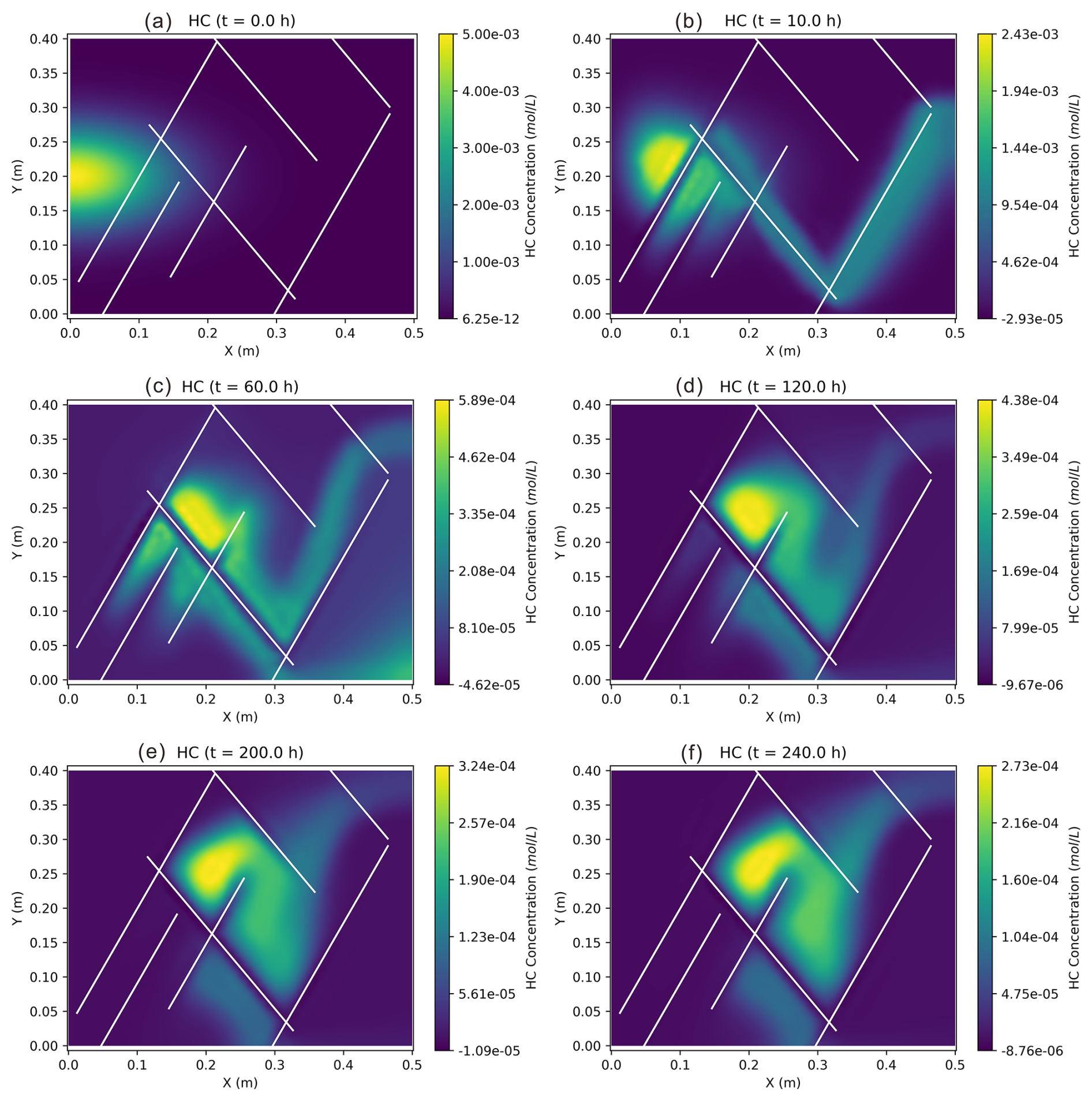
Figure 7 Temporal evolution of Toluene (HC) concentration in the fractured aquifer domain. (a–f) HC concentration distributions at t=0, 10, 60, 120, 200, 240 h, respectively. White lines denote fractures. Colour indicates concentration (mol L⁻¹), showing advection-dispersion coupled with biogeochemical reactions within the matrix and along fracture pathways.

Initial biogeochemical conditions include a toluene (HC) contamination plume centered near the left boundary, with a peak concentration of $\mathrm{5}\times {\mathrm{10}}^{-\mathrm{3}}$ mol L⁻¹ (see Fig. 7a). Background concentrations are set to $\mathrm{2}\times {\mathrm{10}}^{-\mathrm{5}}$ mol L⁻¹ (O₂), $\mathrm{3}\times {\mathrm{10}}^{-\mathrm{5}}$ mol L⁻¹ (NO${}_{\mathrm{3}}^{-}$), $\mathrm{1}\times {\mathrm{10}}^{-\mathrm{5}}$ mol L⁻¹ (SO${}_{\mathrm{4}}^{\mathrm{2}-}$), and 0 mol L⁻¹ (CH₄). The left boundary maintains inflow with fixed background concentrations, while the right acts as an advective outflow. The upper and lower boundaries are impermeable to both groundwater flow and solute transport. Detailed kinetic parameters can be seen in Table 1.

Table 1 Key hydrogeological and transport parameters used in the reactive transport simulation.

The simulation time step is 1 h, for a total of 240 h in this paper. Although a larger time step can be used with a slight sacrifice in accuracy, it is recommended to retrain the model before applying a smaller time step. At each step, species concentrations and hydraulic head fields are exported from COMSOL via MATLAB LiveLink scripts. These outputs serve as inputs to PHYGNET, which predicts the system's chemical evolution. Every 10 steps, CPgPy invokes PHREEQC to recompute full reaction equilibria, ensuring long-term chemical consistency. This hybrid execution scheme balances predictive efficiency with thermodynamic rigor.

4.2 Coupled Reactive Transport Capability of PHYGNET

The spatiotemporal evolution of hydrocarbon (HC) concentration (Fig. 7) demonstrates that PHYGNET successfully participates in the transport process and responds dynamically to flow-driven migration. At early times (t=0–10 h), the HC plume is primarily confined near the source zone and begins to migrate along preferential flow paths controlled by the fracture network. As time progresses (t=60–120 h), the plume elongates and spreads, exhibiting clear anisotropic transport behaviour governed by fracture-dominated advection and transverse dispersion. At later stages (t=200–240 h), the plume morphology stabilizes, with noticeable mass transfer into the surrounding matrix, indicating the onset of diffusion-controlled storage and redistribution.

This continuous evolution from advection-dominated transport to matrix interaction reflects that PHYGNET is not operating as an isolated reaction predictor, but is actively embedded within the transport loop. The model continuously updates concentration fields in response to spatial transport processes, confirming that the coupling between flow, transport, and reaction is effectively maintained.

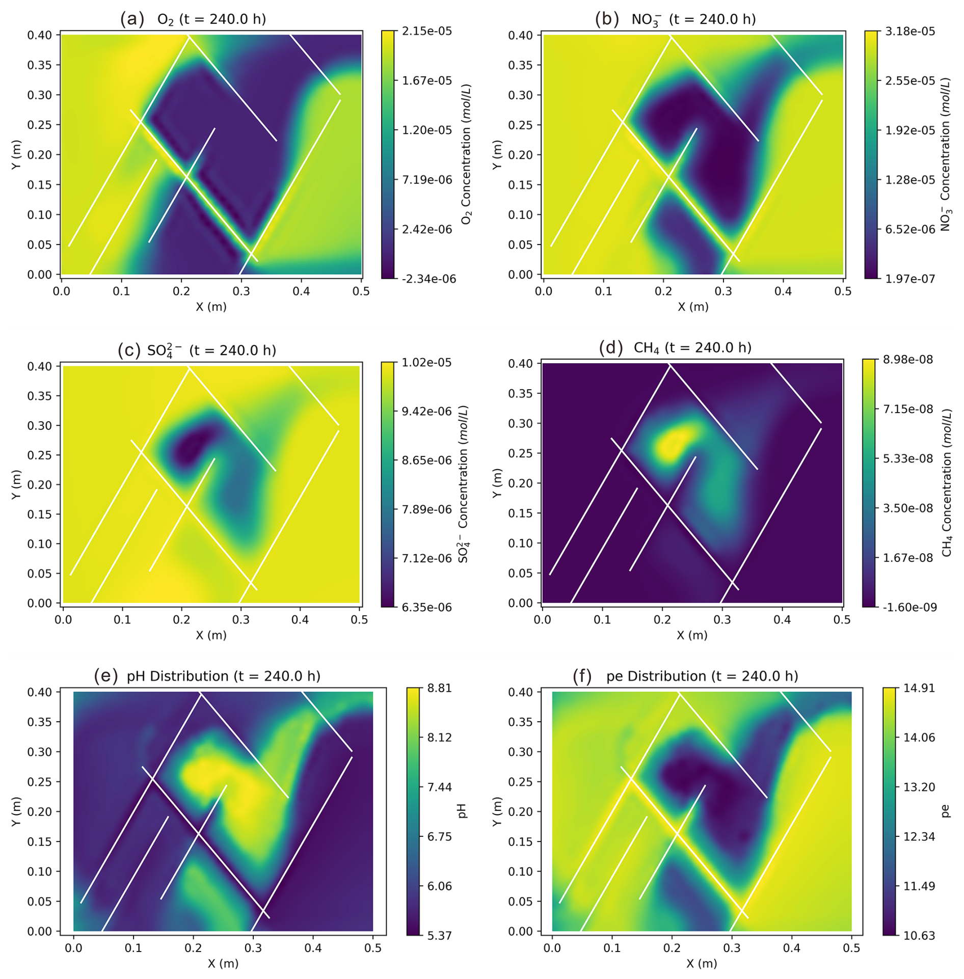
Figure 8 Spatial distributions of major reactive species and geochemical indicators at the final simulation time. (a) Dissolved oxygen (O₂) concentration (mol L⁻¹); (b) Nitrate (NO${}_{\mathrm{3}}^{-}$) concentration (mol L⁻¹); (c) Sulfate (SO${}_{\mathrm{4}}^{\mathrm{2}-}$) concentration (mol L⁻¹); (d) Methane (CH₄) concentration (mol L⁻¹); (e) pH distribution; (f) pe (redox potential) distribution.

The spatial distribution of primary species (Fig. 8) demonstrates that PHYGNET accurately captures the complex redox zonation within the fractured aquifer. The concentration profiles of O₂ and NO${}_{\mathrm{3}}^{-}$ reveal significant depletion zones precisely aligned with the high-permeability fracture network, where hydrocarbon degradation is most intensive. These sharp gradients at the fracture-matrix interface confirm the model's ability to simulate the rapid consumption of oxidants delivered via preferential flow paths, effectively resolving the localized biogeochemical fronts typical of heterogeneous media.

Conversely, the accumulation of CH₄ and the synchronized shifts in pH and pe (Fig. 8d–f) highlight the model's biogeochemical consistency. The peak methane concentrations and reduced pe values are localized within the anaerobic plume core, reflecting the sequential utilization of electron acceptors and the onset of methanogenic conditions. This coherent correlation between oxidant depletion and metabolic by-product formation proves that PHYGNET maintains chemical logic and approximate mass balance, successfully serving as a surrogate for traditional solver while preserving high-fidelity spatial variations across the fractured domain.

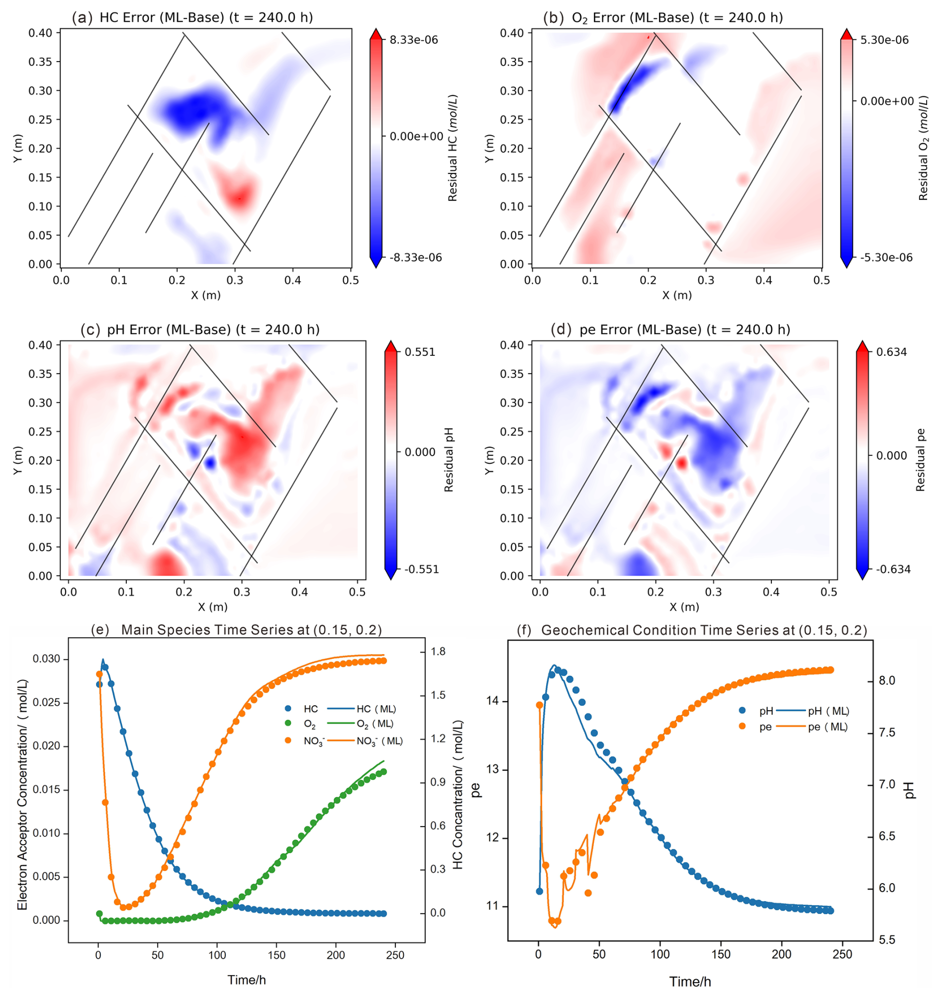
Figure 9 PHYGNET-COMSOL coupling accuracy analysis. (a–d) Present the predicted residuals (ML – baseline) for HC concentration, O₂, pH, and pe, respectively; (e)–(f) show the temporal evolution of major electron acceptors (O₂, NO${}_{\mathrm{3}}^{-}$) alongside pH and pe at representative observation points (0.15, 0.2 m).

The spatial residual distributions at t=240 h (Fig. 9a–d) provide further evidence that the largest accumulated errors tend to occur at the final time step. The HC residuals remain localized and exhibit structured patterns aligned with the plume geometry, particularly near regions of strong concentration gradients and fracture intersections. Similar spatial coherence is observed in the pH and pe residual fields, where deviations are concentrated around chemically active zones rather than being randomly distributed. This indicates that PHYGNET preserves the spatial dependency between transport-driven concentration changes and reaction-induced geochemical responses.

Importantly, the residual patterns of pH and pe are consistent with the underlying redox dynamics. Areas with higher HC concentrations correspond to stronger deviations in redox indicators, reflecting intensified reaction activity. This spatial alignment confirms that PHYGNET correctly translates transport-induced variations in reactant availability into corresponding geochemical state updates, thereby maintaining the internal coupling between species transport and reaction processes.

4.3 Surrogate Efficiency and Robustness

In comprehensive RTM involving kinetic reaction networks, geochemical solvers typically account for the vast majority of the total computational cost due to their complex nonlinear iterative solving mechanisms, and they frequently become the weak link that triggers computational crashes. To quantitatively evaluate the feasibility and performance limits of the PHYGNET surrogate in handling large-scale, three-dimensional site engineering problems, a rigorous benchmark test was conducted. Utilizing realistic chemical state datasets generated during the coupled simulation, we compared the single-step computation time and stability of the serial PHREEQC, parallel PHREEQCRM solver against PHYGNET under a broad range of computational loads (from 10² to 10⁵ grid samples).

It should be acknowledged that this comparison involves an inherent asymmetry in computing hardware, as PHYGNET is executed on GPU whereas PHREEQC and PHREEQCRM rely on CPU. This asymmetry, however, does not undermine the validity of the comparison. The primary source of PHYGNET's efficiency lies not in the hardware itself but in the underlying computational paradigm: once trained, PHYGNET replaces the iterative, nonlinear equilibrium solving required by conventional geochemical solvers with a single forward pass through the network. This structural advantage would hold even on CPU hardware, since the elimination of iterative convergence is what fundamentally reduces computational cost. The use of GPU acceleration further amplifies this advantage by exploiting the inherent parallelism of tensor operations, which is consistent with how most machine learning surrogates are deployed in practice.

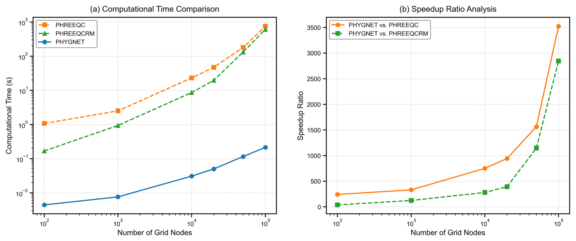
Figure 10 Performance benchmark evaluating the computational efficiency and scalability of the proposed surrogate. (a) Comparison of single-step computational time among PHREEQC, PHREEQCRM and PHYGNET. (b) The corresponding speedup ratios of PHYGNET relative to PHREEQC and PHREEQCRM.

As shown in Fig. 10a, the computational cost of both traditional geochemical solvers increases rapidly with increasing grid nodes. PHREEQC exhibits the most pronounced growth, with the computational time increasing from approximately 1.1 s at 10² grid nodes to 753.6 s at 10⁵ nodes. This rapid increase reflects the accumulated cost of solving nonlinear kinetic equations independently for each grid cell. PHREEQCRM improves the scalability through parallel reaction execution and reduces the computational time to approximately 608.6 s at 10⁵ nodes. However, its parallel efficiency remains constrained by the characteristics of CPU-based computing. Although multiple reaction calculations can be distributed among CPU cores, each individual reaction system still requires iterative nonlinear solving, and the communication and synchronization overhead increases as the number of parallel tasks grows. Consequently, the computational advantage obtained from additional CPU cores gradually diminishes when handling extremely large numbers of grid cells.

In contrast, benefits from the inherent parallelism of GPU-accelerated tensor operations, PHYGNET maintains nearly sub-linear computational growth as the number of grid nodes increases. The inference time increases only from approximately $\mathrm{4.5}\times {\mathrm{10}}^{-\mathrm{3}}$ s at 10² nodes to 0.21 s at 10⁵ nodes. This indicates that once trained, PHYGNET can efficiently process large batches of spatial reaction states without performing expensive nonlinear iterations. The corresponding acceleration ratios are presented in Fig. 10b. At small spatial scales, PHYGNET already provides substantial acceleration compared with both traditional approaches. More importantly, the computational advantage continuously increases with increasing simulation size. At 10⁵ grid nodes, PHYGNET achieves 3588-fold acceleration compared with PHREEQC and 2898-fold acceleration compared with PHREEQCRM. This increasing speedup ratio highlights an important advantage of ML surrogates in large-scale reactive transport modelling: the computational cost of neural inference grows much more slowly than that of conventional reaction solvers.

More notably, as illustrated in Fig. 10b, the speedup ratio of PHYGNET relative to the traditional solver exhibits a significant and continuous upward trend as the number of simulation samples increases. This characteristic reveals a highly practical paradigm for engineering applications. When confronting large-scale 3D site simulations comprising hundreds of thousands or even millions of grid nodes, it is entirely feasible to first employ a traditional solver (e.g., PHREEQC) to generate a limited number of representative small-scale samples to train the surrogate model, and subsequently delegate the remaining, overwhelmingly massive node computation tasks entirely to the trained PHYGNET. Because the surrogate model yields substantial computational dividends from tensor parallelism when processing large-scale data, this “small-sample training, ultra-large-scale inference” strategy effectively offsets the initial time costs incurred during training data generation. This monumental leap in efficiency implies that PHYGNET can compress large-scale uncertainty analyses (e.g., Monte Carlo simulations), which would traditionally require weeks of computation on supercomputing clusters, into a matter of hours on a standard workstation.

Beyond sheer computational speed, the numerical robustness exhibited by the surrogate model is another core value that breaks through the limitations of large-scale RTM applications. When processing real transport data involving multi-electron acceptors and extreme redox gradients (such as fracture-matrix interfaces), the Newton-Raphson iteration method employed by traditional solvers shows extreme fragility. When encountering local stiff kinetics or trace component concentrations approaching numerical limits, this mechanism is highly susceptible to falling into infinite iterative loops or crashing and reporting errors upon reaching the maximum number of iterations. In a complex computational domain with hundreds of thousands of grids, the convergence failure of any single node will inevitably interrupt the entire coupled workflow. As a surrogate model based on continuous function mapping, PHYGNET's inference process is completely decoupled from the iterative approximation mechanics of nonlinear equation systems. Consequently, even under highly heterogeneous chemical gradients in the input data, the network can compute features within a deterministic and extremely minuscule time window. Furthermore, under the dual safeguards of the hard-coded logic gating in the downstream Kinetics Layer and the smooth correction provided by the residual network (MLP), PHYGNET consistently and stably outputs bounded and reasonable results that closely conform to mass conservation and thermodynamic hierarchies. In this benchmark test, even when concurrently subjected to the impact of 100 000 highly heterogeneous solution samples, PHYGNET achieved zero local crashes, zero memory overflows, and zero computational stalls. This quantum leap in efficiency coupled with outstanding numerical robustness fundamentally ensures the continuity and reliability of massive RTM simulations in complex porous and fractured media.

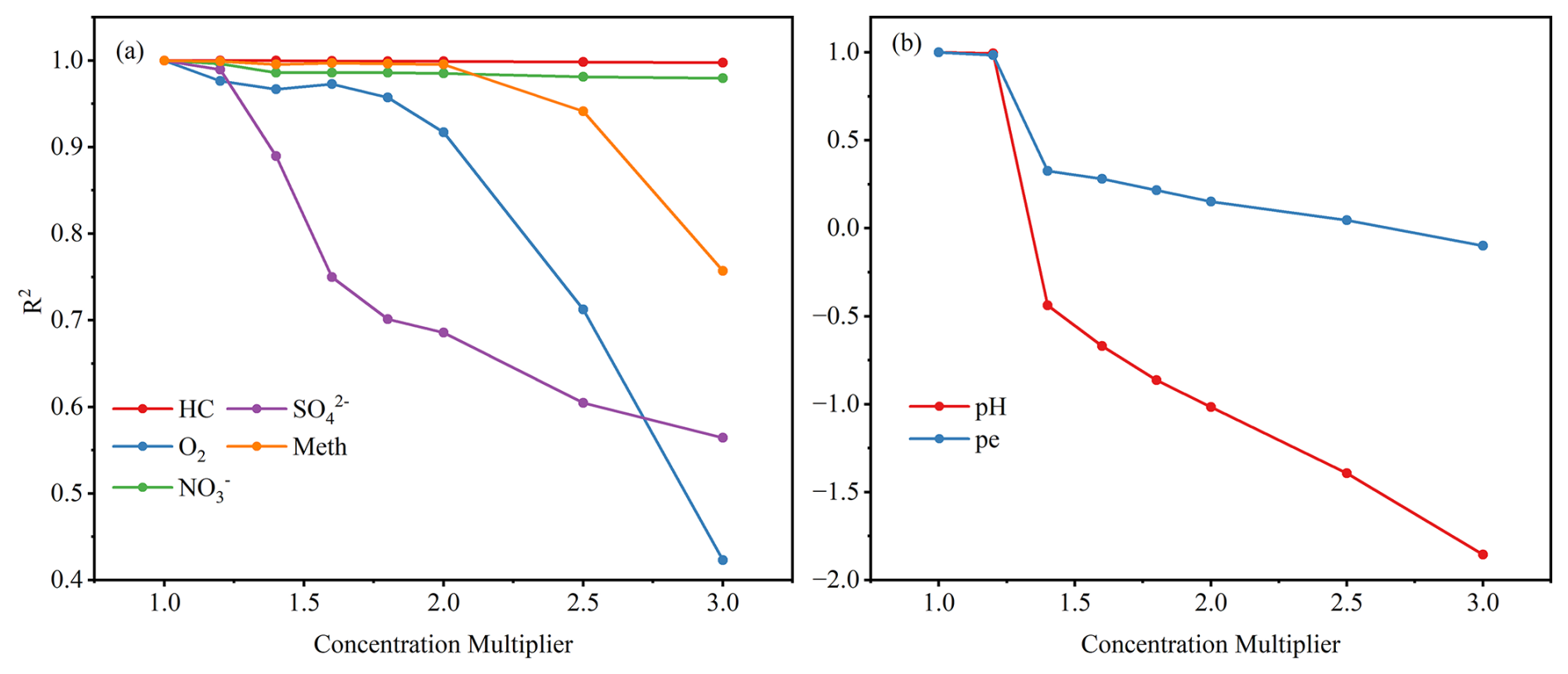
Figure 11 Out-of-distribution (OOD) assessment of PHYGNET under enlarged biochemical concentration ranges (Case A). (a) Variation of prediction accuracy (R²) for reactive species. (b) Variation of R² for environmental state variables, including pH and pe. The results demonstrate that PHYGNET maintains stable predictions for major reactive species under moderate distribution shifts, whereas environmental variables and strongly coupled redox-related species exhibit greater sensitivity under extreme OOD conditions.

To further investigate the extrapolation capability and limitations of PHYGNET under out-of-distribution (OOD) conditions, an additional robustness assessment was conducted by expanding the concentration ranges of all reactive species from 1.0 to 3.0 times the original training distribution (Fig. 11). The results reveal a clear difference in the extrapolation behaviour between reactive species and environmental state variables. For the major reactive species, PHYGNET maintains acceptable predictive performance under moderate distribution shifts, with R² values remaining above 0.7 when the concentration expansion factor is below 1.8. However, the prediction accuracy gradually deteriorates under more extreme perturbations, indicating that excessive extrapolation beyond the training distribution can introduce considerable uncertainty. In contrast, environmental variables (pH and pe) exhibit a much stronger sensitivity to OOD conditions and retain reliable predictions only within a narrower range (approximately $\le \mathrm{1.4}\times$). This discrepancy originates from the current hybrid architecture: the differentiable kinetic layer explicitly imposes physical constraints on species concentrations through Monod-type reaction formulations and mass-transfer relationships, whereas environmental state variables are mainly corrected by the residual MLP without equivalent mechanistic constraints. Consequently, although PHYGNET provides stable predictions within the sampled chemical regime, its reliability may decrease when applied to substantially different site conditions. Therefore, for practical field-scale applications, sufficient representative observations should be collected beforehand to characterize the statistical distribution of the target system, ensuring that the training dataset adequately covers the expected range of biochemical conditions and avoiding excessive extrapolation during model deployment.

4.4 Surrogate Interpretability

To investigate how PHYGNET infers latent kinetic parameters from sparse concentration fields without explicit supervision, we applied SHAP analysis (Lundberg and Lee, 2017) to the predicted logarithmic rate constants (logk_max,i) and the residual correction terms. The results are analysed as follows.

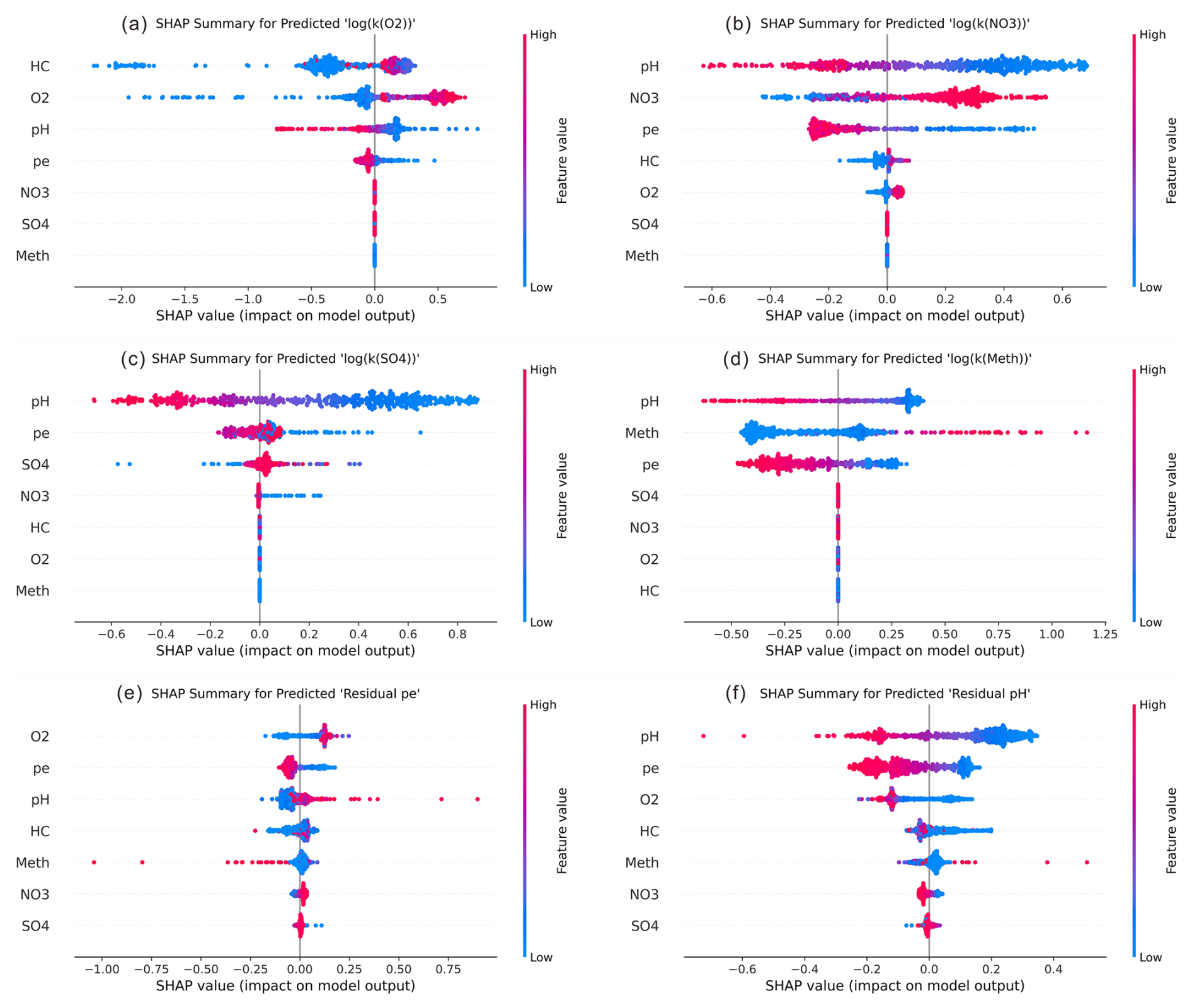
Figure 12 SHAP summary plots revealing the autonomous learning of biogeochemical mechanisms by PHYGNET. The analysis decomposes the drivers for (a–d) predicted kinetic rate parameters (logk_max,i) and (e–f) residual corrections. (a) Aerobic respiration is correctly driven by substrate availability (O₂ and HC). (b–d) For anaerobic pathways, theoretical inhibitors (e.g., O₂ for denitrification) exhibit positive SHAP contributions. (e–f) Residual corrections for pH and pe show a negative correlation with their respective state variables.

The aerobic pathway provides a clear example of substrate-driven behaviour. For the aerobic respiration rate constant log($k_{{\mathrm{O}}_{\mathrm{2}}}$) (Fig. 12a), the SHAP summary plot shows strong positive contributions associated with high concentrations of dissolved O₂ and HC. Regions containing both electron donors and electron acceptors therefore receive the largest upward shifts in predicted rate constants. This pattern aligns closely with classical Monod kinetics, in which reaction potential is maximized when both substrates are abundant (Monod, 1949). Consistent with this principle, the GNN component correctly identifies the hydrocarbon plume core as the region of highest metabolic activity, even under strong spatial heterogeneity.

In contrast, anaerobic pathways including denitrification and sulfate reduction (Fig. 12b–c) display an apparently counterintuitive SHAP pattern: inhibitors such as O₂ and NO${}_{\mathrm{3}}^{-}$ show positive contributions to the predicted rate constants. For instance, higher concentrations of O₂ correlate with larger log($k_{{\mathrm{SO}}_{\mathrm{4}}^{\mathrm{2}-}}$) values, despite the fact that sulfate reduction should be thermodynamically suppressed under oxidizing conditions. This behaviour does not necessarily indicate model error; rather, it reflects the cooperative structure of PHYGNET's hybrid architecture. The GNN serves as a “resource recognizer”, leveraging persistent spatial correlations in the plume. Zones with high concentrations of supposed inhibitors often coincide with the advancing plume front, where HC and other reactants remain abundant. The GNN learns to interpret these high-concentration signals as markers of high reaction potential, producing correspondingly high estimates of the maximum rate constant. Crucially, these predictions do not directly determine the final reaction rate. The downstream physics-based kinetics layer imposes explicit Monod inhibition terms, which strictly enforce thermodynamic hierarchy. Even if the GNN predicts a high k_max in oxic zones, the kinetics layer mathematically drives the actual reaction rate toward zero. This synergy effectively separates the tasks of “locating potential reactivity” and “enforcing thermodynamic feasibility”, reducing the learning burden and improving stability in kinetic reaction systems.

SHAP analysis of the residual correction terms for pH and pe (Fig. 12e–f) further reveals a consistent negative correlation pattern, when the state variable is high, the residual network tends to output a negative adjustment. This indicates that the lightweight MLP acts as a “steady-state buffer”, mimicking acid-base and redox buffering processes commonly observed in natural waters. By compensating for linearization errors in the physics layer, the residual network keeps the predicted system within chemically reasonable bounds and prevents long-term numerical drift.

Taken together, these interpretability results demonstrate that PHYGNET possesses strong physical reasoning capabilities. Its architecture successfully decouples the tasks of detecting spatial patterns of reaction potential (handled by the GNN) and enforcing biogeochemical constraints (handled by the physics layer), while the residual network provides fine-scale stabilizing adjustments. This hybrid mechanism enables accurate, stable, and interpretable simulation of reactive transport in complex multi-electron-acceptor environments.

5 Conclusions

This study introduces PHYGNET, a physically integrated Graph Neural Network (GNN) framework designed to serve as an efficient, interpretable, and highly robust surrogate for biogeochemical solvers in reactive transport models (RTMs). By integrating a metabolic-structured GNN architecture with an explicit Monod-based kinetic physics layer and a residual corrector, PHYGNET successfully overcomes the intrinsic limitations of pure data-driven black-box models. It accurately captures the stiff, nonlinear dynamics of microbially-mediated kinetic reaction degradation systems while enforcing stoichiometric mass conservation within the kinetics layer, improving the mass-balance consistency of the final outputs, and preserving thermodynamic hierarchies.

Interpretability analyses via SHAP confirm that PHYGNET captures intuitive and mechanistically consistent trends in how local substrate concentration and redox conditions affect reaction rates. The GNN effectively acts as a spatial “resource recognizer” for metabolic reaction potentials, while the downstream physics layer guarantees thermodynamic feasibility, providing a transparent and trustworthy ML-physics synergy.

When embedded into a COMSOL-coupled RTM framework, PHYGNET demonstrated exceptional performance in simulating complex plume evolution and biological redox zonation within a highly heterogeneous fractured aquifer. Crucially, rigorous benchmark testing revealed that PHYGNET could alleviate the computational burden associated with high-dimensional systems and numerical stiffness that plague traditional solvers. While conventional tools such as PHREEQC suffer from super-linear time penalties and convergence failures at engineering scales, PHYGNET exploits tensor parallelism to maintain stable sub-linear scaling. At a massive scale of 100 000 grid nodes, the surrogate achieved an unprecedented 3588-fold computational acceleration with zero numerical crashes. Furthermore, the continuous upward trend of the speedup ratio with increasing computational scale establishes a highly practical engineering paradigm, utilizing a small number of samples generated by traditional solvers for training, followed by ultra-large-scale inference on millions of nodes. This strategy effectively offsets the initial time costs of data generation and maximizes the dividends of tensor parallelism.

Beyond efficiency gains, the model's modular design supports easy adaptation to new transport boundary conditions, contaminants, and microbial metabolic pathways, offering broad utility for large-scale environmental bioremediation simulations. By compressing the computational time of large-scale RTMs from weeks to a matter of hours, this work provides a promising pathway for addressing previously intractable tasks (such as high-resolution 3D site modelling, real-time remediation optimization, and comprehensive uncertainty quantification), marking a significant step forward in the real-world application of reactive transport modelling.

Despite these capabilities, we acknowledge certain limitations in the current study that outline the trajectory for future research. Presently, the performance and stability of the PHYGNET framework have been rigorously validated primarily within synthetic, albeit highly heterogeneous, 2D fractured domains. Additionally, the current physics layer is exclusively tailored for Monod-type biological kinetics and does not yet explicitly resolve concurrent inorganic processes such as mineral dissolution-precipitation. Therefore, our forthcoming work will focus on expanding the differentiable physics library to encompass a wider range of geochemical formulations, and deploying PHYGNET at a full-scale, three-dimensional real-world field site.