A data-driven method coupling multiple physical constraints for correcting structural errors in groundwater contaminant transport models

Model structural errors are pervasive in groundwater contaminant transport modeling under complex environmental conditions, hindering accurate prediction of contamination transport. Data-driven methods (DDMs) coupled with physical constraints provide an effective approach for correcting structural errors and improving prediction. However, in multicomponent reactive transport systems, multiple physical mechanisms must be satisfied simultaneously, whereas existing DDMs have limited capacity to effectively couple multiple physical constraints. To address this challenge, this study proposes a general method for correcting structural errors in groundwater models. A combined likelihood function is constructed and sub-likelihood weights are dynamically updated to effectively couple multiple physical constraints. The method is evaluated using a synthetic three-dimensional tetrachloroethylene reactive transport simulation and a cadmium-phosphate cotransport sand column experiment. These tests systematically assess the effects of coupling single versus multiple physical constraints on structural error correction and predictive performance. The results show that coupling multiple constraints can constrain parameter identification, reduce predictive uncertainty, and more comprehensively improve model predictions. Appropriate physical constraints function analogously to incorporating additional observations. Moreover, coupling multiple physical constraints results in a simpler form of structural error in the calibrated groundwater model, making it easier to characterize, thereby enhancing prediction accuracy and physical consistency. The proposed dynamic updating and stopping criterion of sub-likelihood weights maintains a balance between multiple physical constraints and observations, improving the robustness of parameter identification and constraint enforcement. Overall, the proposed DDM coupled with multiple physical constraints provides a general framework for correcting structural errors in complex groundwater contaminant transport models.

1 Introduction

Numerical groundwater models are essential tools for predicting contaminant transport processes in groundwater and play a critical role in risk assessment and remediation decision-making at contaminated sites (Kim et al., 2026; Wen et al., 2025). With increasing demands for efficient and sustainable remediation of groundwater contamination, improving the predictive accuracy of complex migration and transformation processes of contaminants in aquifers, together with conducting reliable uncertainty analysis, has become imperative (Zeeshan and Ruhl, 2023). Although extensive studies have focused on parameter uncertainty (Hendrikx et al., 2026; Engdahl, 2025), comparatively limited attention has been devoted to model structural error. Owing to the complexity of groundwater systems and limitations in human understanding, constructed groundwater models are often simplified or even misspecified representations of real systems, resulting in the widespread presence of structural error (Refsgaard et al., 2006; Neuman and Wierenga, 2003). Such structural deficiencies lead to systematic errors in model predictions (Watson et al., 2013; Ye et al., 2004), thereby reducing the reliability of prediction-informed decisions (Sun et al., 2021; Gupta et al., 2012).

In recent years, data-driven methods (DDMs) have been widely employed to correct model structural errors and enhance the predictive performance of physics-based models (Yu et al., 2022; Hu et al., 2021; Kasiviswanathan et al., 2019; Pathiraja et al., 2018). These approaches construct an error-correcting complementary model to explicitly account for systematic discrepancies in model predictions, such that the corrected predictions consist of the physical model, the structural error model, and the measurement error (Xu et al., 2017; Xu and Valocchi, 2015). Previous studies have demonstrated that applying DDMs to correct structural error can substantially improve the predictive accuracy of groundwater head, soil moisture, and contaminant concentration (Pan et al., 2023; Sun et al., 2021; Zhang et al., 2019). However, the error-correction models constructed by these approaches remain essentially black-box statistical models that lack necessary physical constraints. Consequently, they may yield predictions that violate fundamental physical principles, such as contaminant concentrations exceeding physically plausible ranges or violating mass conservation, thereby weakening the plausibility and reliability of the predictions.

Incorporating physical constraints into DDMs provides an effective means of enhancing the physical consistency of predictions. Previous studies have parameterized physical constraints and formulated them as constraint conditions in optimization problems to achieve coupling of physical mechanisms (Ayensa-Jiménez et al., 2018; He and Xiu, 2016). However, when multiple physical constraints are considered simultaneously, the number of unknown parameters may exceed the number of physical constraints, thereby increasing predictive uncertainty. Wu et al. (2024) incorporated the energy conservation constraint into parameter identification by jointly considering the accumulated violation of the energy conservation constraint and prediction error. Nevertheless, under multiple physical constraints, different physical constraints may compete with one another, making it difficult for predictions to simultaneously satisfy all physical mechanisms. In the groundwater field, Xu and Valocchi (2015) coupled model predictions with the water balance equation through recalibration. However, imposing multiple physical constraints through recalibration may drive the physical model parameters to overfit in order to satisfy all constraints and result in numerical instability or infeasible solutions, thereby limiting the applicability of the approach. Overall, although existing methods can couple a single physical constraint, there remains a lack of a general method capable of simultaneously and effectively coupling multiple physical constraints.

The rapid development of physics-informed machine learning (PIML) offers a potential pathway for coupling multiple physical constraints. PIML typically incorporates physical mechanisms at three stages: during data preparation, by selecting or augmenting training data based on physical constraints (Melching et al., 2023; Zhang et al., 2021); during model construction, by introducing physics-constrained layers (Mendenhall et al., 2024; Saha et al., 2021); and during model training, by designing specific loss functions or inference algorithms to enforce physical constraints (Zhang et al., 2022, 2023; Guo et al., 2022). To date, PIML has been widely applied in hydrology, engineering, and materials science (Cao and Weng, 2024; Cooper et al., 2023; Lu et al., 2022), demonstrating its potential to integrate multiple physical constraints simultaneously, such as mass balance, monotonicity, and boundary conditions. However, existing PIML approaches still face limitations in correcting model structural errors. This is primarily because PIML typically constrains only the error-correction model itself rather than the entire error-correction process. As a result, the corrected predictions, which consist of the physical model, the structural error model, and measurement error, may still violate fundamental physical principles. Moreover, existing PIML approaches lack effective strategies for selecting appropriate physical constraints tailored to model structural errors, further limiting their potential to enhance predictive reliability and physical consistency.

By constructing a combined likelihood function within a Bayesian uncertainty analysis framework, Tian et al. (2026) successfully coupled Gaussian process regression with a mass conservation constraint to correct structural errors in groundwater models. However, in complex groundwater systems involving multicomponent reactive transport processes, it is often necessary to simultaneously constrain the physical mechanisms associated with multiple components. In such cases, because different physical constraints represent distinct physical meanings, the magnitudes of their corresponding likelihood functions may differ by several orders of magnitude. Simply combining these likelihood functions may cause certain constraints to dominate or be neglected, thereby hindering the effective coupling of multiple physical constraints. Therefore, developing a general structural error correction method capable of coupling multiple physical constraints is essential for improving the accuracy and reliability of transport simulations in complex groundwater contamination systems.

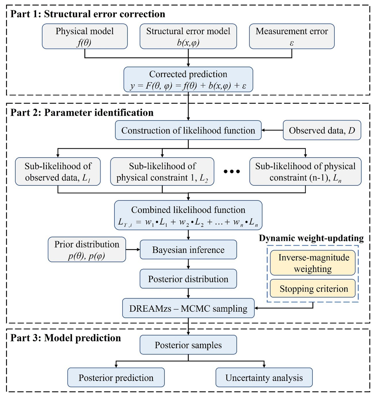
This study proposes a general physics-constrained DDM framework that simultaneously embeds multiple physical constraints into the structural error correction process. The constructed combined likelihood function consists of two components: a conventional likelihood function that quantifies the fit between predictions and observations, and a second component comprising multiple sub-likelihood functions that measure the extent to which predictions satisfy individual physical constraints. In addition, an adaptive weight-updating strategy with a stopping criterion is introduced. During parameter identification, the sub-likelihood function weights are updated according to their relative magnitudes, thereby achieving a reasonable balance between data fitting and multiple physical constraints. The effectiveness of the proposed method is evaluated using two groundwater contaminant transport simulation cases: a synthetic three-dimensional tetrachloroethylene (PCE) reactive transport simulation and a cadmium-phosphate cotransport sand column experiment. The results indicate that the proposed physics-constrained DDM framework effectively couples multiple physical constraints, significantly improving predictive performance of groundwater models and providing a reliable basis for risk assessment and remediation decision-making at complex contaminated sites.

The remainder of this paper is organized as follows. Section 2 presents the Bayesian data-driven framework, the formulation for coupling multiple physical constraints, and the weight-updating strategy with a stopping criterion. Sections 3 and 4 describe the configurations of the two case studies and the implementation of the physics-constrained DDM framework, respectively. Section 5 presents and discusses the results. Section 6 summarizes the main conclusions.

2 Methods

2.1 Bayesian Data-driven Methods

For a groundwater system, the observed data D can be expressed as (Kennedy and O'Hagan, 2001):

$$\begin{array}{}\text{(1)}& D=f\left(\mathit{\theta }\right)+b(x,\mathit{\phi })+\mathit{ϵ}\end{array}$$

where f denotes the groundwater model and θ represents the model parameters. b(x, φ) denotes the systematic prediction error described by Gaussian process regression (GPR), where x and φ represent the inputs and hyperparameters of the GPR model, respectively. ϵ denotes random measurement error.

In this study, Gaussian process regression (GPR) is employed to construct the structural error correction model b(x,φ). It is assumed that b(x,φ) follows a multivariate Gaussian distribution N(μ,C), which is fully characterized by the mean function μ(x)=E(b(x)) and the covariance function $k(x,x{}^{\prime })=E\left(\right(b\left(x\right)-\mathit{\mu }\left(x\right)\left)\right(b\left(x{}^{\prime }\right)-\mathit{\mu }\left(x{}^{\prime }\right)\left)\right)$. The mean function μ is set to zero, and a Matérn covariance kernel with smoothness parameter $\mathit{\nu }=\mathrm{5}/\mathrm{2}$ is adopted (Rasmussen and Williams, 2005):

$$\begin{array}{}\text{(2)}& \begin{array}{rl}{C}_{i,j}=k(x_i,x_j)& ={\mathit{\sigma }}^{\mathrm{2}}\left(\mathrm{1}+{\displaystyle \frac{\sqrt{\mathrm{5}}(x_i-x_j{)}^T(x_i-x_j)}{\mathit{\lambda }}}\right.\\ & \left.+{\displaystyle \frac{\mathrm{5}\left(\right(x_i-x_j{)}^T(x_i-x_j){)}^{\mathrm{2}}}{\mathrm{3}{\mathit{\lambda }}^{\mathrm{2}}}}\right)\\ & \times \exp \left(-{\displaystyle \frac{(x_i-x_j{)}^T(x_i-x_j)}{{\mathit{\lambda }}^{\mathrm{2}}}}\right)+{\mathit{\sigma }}_{\mathit{ϵ}}^{\mathrm{2}}I\end{array}\end{array}$$

where I denotes an indicator function that equals 1 if i=j and 0 otherwise. The hyperparameter φ consists of λ, σ² and ${\mathit{\sigma }}_{\mathit{ϵ}}^{\mathrm{2}}$, where λ denotes the characteristic length scale, σ² represents the marginal variance of b(x), and ${\mathit{\sigma }}_{\mathit{ϵ}}^{\mathrm{2}}$ denotes the variance of measurement error.

The groundwater model parameters θ and the GPR hyperparameters φ are commonly assumed to be independent in the prior distribution. Accordingly, θ and $\mathit{\phi }(\mathit{\lambda },{\mathit{\sigma }}^{\mathrm{2}},{\mathit{\sigma }}_{\mathit{ϵ}}^{\mathrm{2}})$ can be jointly calibrated (Xu and Valocchi, 2015; Xu et al., 2017; Pan et al., 2020). Based on Bayes' theorem, the posterior distribution can be expressed as:

$$\begin{array}{}\text{(3)}& p(\mathit{\theta },\mathit{\phi }\left|D\right.)\propto p(D\left|\mathit{\theta }\right.,\mathit{\phi })p\left(\mathit{\theta }\right)p\left(\mathit{\phi }\right)\end{array}$$

where p(θ) and p(φ) denote the prior distributions of the physical parameters θ and the hyperparameters φ, respectively, and p(D|θ,φ) represents the likelihood function. In this study, a commonly used Gaussian likelihood function is adopted, and its logarithmic form can be written as:

$$\begin{array}{}\text{(4)}& \begin{array}{rl}& \log \left(p\right(D\left|\mathit{\theta },\mathit{\phi }\right.\left)\right)=-{\displaystyle \frac{\mathrm{1}}{\mathrm{2}}}(D-f-\mathit{\mu }{)}^T\\ & \sum ^{-\mathrm{1}}(D-f-\mathit{\mu })-{\displaystyle \frac{\mathrm{1}}{\mathrm{2}}}\log \left|\sum \right|-{\displaystyle \frac{N}{\mathrm{2}}}\log \mathrm{2}\mathit{\pi }\end{array}\end{array}$$

where μ denotes the mean of the systematic prediction error, ∑ represents the error covariance matrix, and N is the number of observations.

Since the posterior distribution p(θ,φ|D) is generally intractable to evaluate analytically, Markov chain Monte Carlo (MCMC) simulation is employed to generate posterior samples of the physical parameters θ and the GPR hyperparameters φ. In this study, the Differential Evolution Adaptive Metropolis (DREAMzs) algorithm is adopted for MCMC sampling, which has been widely applied in groundwater inverse modeling and uncertainty analysis.

Based on the posterior samples of θ and φ obtained from MCMC simulation, predictions of the physical model f and the structural error model b can be generated for a new input x^*, denoted as f^*(θ) and $b^{*}(x^{*},\mathit{\phi })$, respectively. The latter can be expressed as:

$$\begin{array}{}\text{(5)}& b^{*}\left|D-f,D,D^{*}\sim N(\stackrel{\mathrm{‾}}{b^{*}},{\mathbf{C}}_b(b^{*}\left)\right)\right.\end{array}$$

where,

$$\begin{array}{}\text{(6)}& {\displaystyle }{b}^{*}={\mathit{\mu }}^{*}+{\mathbf{C}}^{*T}{\mathbf{C}}^{-\mathrm{1}}(D-f-\mathit{\mu })\text{(7)}& {\displaystyle }{\mathbf{C}}_b\left(b^{*}\right)={\mathbf{C}}^{**}-{\mathbf{C}}^{*T}{\mathbf{C}}^{-\mathrm{1}}{\mathbf{C}}^{*}\end{array}$$

where $\stackrel{\mathrm{‾}}{b^{*}}$ denotes the posterior mean, C_b(b^*) represents the posterior covariance matrix, and μ^* denotes the prior mean $\mathit{\mu }(x^{*},\mathit{\phi })$. The prior covariance matrices C^* and ${\mathbf{C}}^{**}$ are defined as ${\mathbf{C}}_{i,j}^{*}=f(x_i,x_j^{*})$ and ${\mathbf{C}}_{i,j}^{**}=f(x_i^{*},x_j^{*})$, respectively.

The final corrected prediction D^* can be expressed as:

$$\begin{array}{}\text{(8)}& {\mathit{D}}^{*}=f^{*}+b^{*}+{\mathit{ϵ}}^{*}\end{array}$$

where f^*, b^* and ϵ^* denote the predictions of the groundwater model, the structural error model, and the measurement error at x^*, respectively.

2.2 Likelihood Function-based Coupling of Physical Constraints

In practical applications, predictions of groundwater contaminant transport simulations are typically required to satisfy multiple key physical constraints, such as contaminant mass conservation and non-negativity of concentration. In this study, each physical constraint is represented by a set of functions:

$$\begin{array}{}\text{(9)}& {\displaystyle }G\left(y\right)={\left[g_{\mathrm{1}}\left(y\right),g_{\mathrm{2}}\left(y\right),\mathrm{\dots },g_{n_c}\left(y\right)\right]}^T=[\mathrm{0},\mathrm{0},\mathrm{\dots },\mathrm{0}{]}^T\text{(10)}& {\displaystyle }Z\left(y\right)={\left[z_{\mathrm{1}}\left(y\right),z_{\mathrm{2}}\left(y\right),\mathrm{\dots },z_{n_f}\left(y\right)\right]}^T=[\mathrm{0},\mathrm{0},\mathrm{\dots },\mathrm{0}{]}^T\end{array}$$

where y denotes the corrected prediction (i.e., the sum of the physical model, the structural error model, and the measurement error), which is a function of the parameters θ and φ, i.e., $y=F(\mathit{\theta },\mathit{\phi })$. $g_i\left(y\right),i=\mathrm{1},\mathrm{2},\mathrm{\dots },n_c$ represent the equality constraints, where n_c denotes the number of equality constraints. $z_i\left(y\right),i=\mathrm{1},\mathrm{2},\mathrm{\dots },n_f$ represent the inequality constraints, where n_f denotes the number of inequality constraints. The zero matrix on the right-hand side indicates that the corrected predictions are required to satisfy the corresponding physical constraints at each observation time.

The equality constraints are assumed to follow a zero-mean Gaussian distribution, and Eq. (9) can therefore be expressed as:

$$\begin{array}{}\text{(11)}& G\left(y\right)=G\left(F\right(\mathit{\theta },\mathit{\phi }\left)\right)\sim N\left(\mathrm{0},\sum _c\right)\end{array}$$

where ∑_c is a diagonal covariance matrix used to control the strictness of constraints (Wu et al., 2019).

Therefore, a likelihood function can be constructed to quantify the extent to which the corrected predictions satisfy the equality constraints, conditional on the parameters θ and φ:

$$\begin{array}{}\text{(12)}& \begin{array}{rl}p\left(G\right(y)=& \mathrm{0}\left|\mathit{\theta },\mathit{\phi }\right.)={\displaystyle \frac{\mathrm{1}}{\sqrt{(\mathrm{2}\mathit{\pi }{)}^{n_c}\left|{\sum }_c\right|}}}\\ & \exp \left(-{\displaystyle \frac{\mathrm{1}}{\mathrm{2}}}G\left(F\right(\mathit{\theta },\mathit{\phi }\left){)}^T\sum _c^{-\mathrm{1}}G\right(F(\mathit{\theta },\mathit{\phi }))\right)\end{array}\end{array}$$

For the inequality constraints, Eq. (10) can be transformed into the corresponding equality constraints as:

$$\begin{array}{}\text{(13)}& min(\mathrm{0},Z(y\left)\right)=\mathrm{0}\end{array}$$

Similarly, under the assumption of a zero-mean Gaussian distribution, Eq. (13) can be written as:

$$\begin{array}{}\text{(14)}& min(\mathrm{0},Z(y\left)\right)\sim N\left(\mathrm{0},\sum _f\right)\end{array}$$

The corresponding likelihood function can be constructed as:

$$\begin{array}{}\text{(15)}& \begin{array}{rl}& p\left(Z\right(y)\ge \mathrm{0}\left|\mathit{\theta },\mathit{\phi }\right.)={\displaystyle \frac{\mathrm{1}}{\sqrt{(\mathrm{2}\mathit{\pi }{)}^{n_f}\left|{\sum }_f\right|}}}\\ & \exp \left(-{\displaystyle \frac{\mathrm{1}}{\mathrm{2}}}{\left[min(\mathrm{0},Z(y\left)\right)\right]}^T\sum _f^{-\mathrm{1}}min(\mathrm{0},Z(y\left)\right)\right)\end{array}\end{array}$$

Accordingly, the posterior distribution conditional on both the observational data and multiple physical constraints (including the equality and inequality constraints described above) can be expressed as:

$$\begin{array}{}\text{(16)}& \begin{array}{rl}p(\mathit{\theta },\mathit{\phi }\left|D,G\left(y\right)\right.& =\mathrm{0},Z\left(y\right)\ge \mathrm{0})\propto p(D,G\left(y\right)\\ & =\mathrm{0},Z\left(y\right)\ge \mathrm{0}\left|\mathit{\theta },\mathit{\phi }\right.\left)p\right(\mathit{\theta }\left)p\right(\mathit{\phi })\\ & =p\left(D\left|\mathit{\theta },\mathit{\phi }\right.\right)p\left(G\right(y)\\ & =\mathrm{0}\left|\mathit{\theta },\mathit{\phi }\right.\left)p\right(Z\left(y\right)\ge \mathrm{0}\left|\mathit{\theta },\mathit{\phi }\right.\left)p\right(\mathit{\theta }\left)p\right(\mathit{\phi })\end{array}\end{array}$$

where p(D|θ,φ) corresponds to the likelihood function that quantifies the fit between the predictions and the observational data, as given in Eq. (4), $p\left(G\right(y)=\mathrm{0}\left|\mathit{\theta },\mathit{\phi }\right.)$ and $p\left(Z\right(y)\ge \mathrm{0}\left|\mathit{\theta },\mathit{\phi }\right.)$ correspond to the likelihood functions incorporating the equality and inequality constraints defined in Eqs. (12) and (15), respectively.

This formulation can be further generalized, and Eq. (16) is equally applicable when additional physical constraints are incorporated. In this case, the total log-likelihood function can be expressed as the sum of the log-likelihoods of the individual sub-likelihood functions:

$$\begin{array}{}\text{(17)}& L_{\mathrm{T}}=L_{\mathrm{1}}+L_{\mathrm{2}}+L_{\mathrm{3}}\mathrm{\dots }+L_n\end{array}$$

where L_T denotes the total likelihood, L₁ represents the likelihood associated with the predictions, and $L_{\mathrm{2}},L_{\mathrm{3}},\mathrm{\dots },L_n$ denote the likelihood functions corresponding to different physical constraints.

Therefore, MCMC sampling is performed based on the combined likelihood function (Eq. 17) to jointly identify the posterior distributions of the groundwater model parameters θ and the GPR hyperparameters φ.

2.3 Dynamic Weight-updating Strategy with a Stopping Criterion

Because different sub-likelihood functions correspond to distinct physical meanings, their magnitudes may differ substantially, leading to unequal competition among the sub-likelihood functions. Therefore, it is necessary to assign weights to the sub-likelihood functions and dynamically update them according to their relative magnitudes. In this study, an inverse-magnitude weighting method is adopted to weight the sub-likelihood functions as follows (Guger et al., 2020; Li et al., 2018):

$$\begin{array}{}\text{(18)}& L_{\mathrm{T},i}=w_{\mathrm{1},i}\cdot L_{\mathrm{1},i}+w_{\mathrm{2},i}\cdot L_{\mathrm{2},i}+\mathrm{\dots }+w_{n,i}\cdot L_{n,i}\end{array}$$

where $L_{\mathrm{1},i},L_{\mathrm{2},i},\mathrm{\dots },L_{n,i}$ denote the n sub-likelihood functions obtained at the i-th iteration of the Bayesian updating process under the scenario with multiple physical constraints, and $w_{\mathrm{1},i},w_{\mathrm{2},i},\mathrm{\dots },w_{n,i}$ denote the corresponding weights. The dynamic weight-updating procedure is described as follows:

First, the mean of each sub-likelihood function is calculated as follows:

$$\begin{array}{}\text{(19)}& L_{\mathrm{avg},i}={\displaystyle \frac{{\sum }_{j=\mathrm{1}}^n{L}_{j,i}}{n}}\end{array}$$

Then, the initial unnormalized weights are computed:

$$\begin{array}{}\text{(20)}& w_{j,i}^{\prime }={\displaystyle \frac{L_{\mathrm{avg},i}}{L_{j,i}}},j=\mathrm{1},\mathrm{2},\mathrm{\dots },n\end{array}$$

Finally, the weights are normalized:

$$\begin{array}{}\text{(21)}& w_{j,i}={\displaystyle \frac{w_{j,i}^{\prime }}{{\sum }_{k=\mathrm{1}}^n{w}_{k,i}^{\prime }}},j=\mathrm{1},\mathrm{2},\mathrm{\dots },n\end{array}$$

During the dynamic weight-updating process, determining when to terminate weight updating is crucial for ensuring the stability and convergence of MCMC sampling. In this study, a stopping criterion derived from multi-objective evolutionary algorithms is introduced (Abu Doush et al., 2023; Kadhar and Baskar, 2018), whereby weight updating is terminated when the variance of weight changes remains stable within a specified iteration window. Since multiple Markov chains are employed, the weights of the sub-likelihood functions are updated separately for each chain during the burn-in period based on its own evolution. Once the stopping criterion is satisfied, a common set of fixed sub-likelihood weights is used for subsequent sampling across all chains. The procedure is as follows:

1. After the ith iteration, compute the weight $w_{j,i}^r$ of the jth sub-likelihood function for the rth chain.

2. Compute the change in each weight between two consecutive iterations $\mathrm{\Delta }{w}_{j,i}^r=\left|w_{j,i}^r-w_{j,i-\mathrm{1}}^r\right|$.

3. Over the most recent γ iterations, compute the variance of the weight changes for each sub-likelihood function and each chain as $V_{j,\mathit{\gamma }}^r=\mathrm{Variance}(\mathrm{\Delta }{w}_{j,i-\mathit{\gamma }+\mathrm{1}}^r,\mathrm{\Delta }{w}_{j,i-\mathit{\gamma }+\mathrm{2}}^r,\mathrm{\dots },\mathrm{\Delta }{w}_{j,i}^r)$. The maximum value ${\mathrm{MV}}_{j^{*},\mathit{\gamma }}^{r^{*}}$ is then recorded, and the corresponding weight change is denoted as $M\mathrm{\Delta }{w}_{j^{*},i}^{r^{*}}$, which is then used in the subsequent χ² test.

4. A χ² test is conducted to statistically assess whether $M\mathrm{\Delta }{w}_{j^{*},i}^{r^{*}}$ over the recent γ iterations is smaller than the prescribed tolerance variance (Tol_fun). The test statistic is given by:

   $$\begin{array}{}\text{(22)}& \begin{array}{rl}& \mathit{\chi }\left(M\mathrm{\Delta }{w}_{j^{*},i}^{r^{*}}\right)=\\ & {\displaystyle \frac{\mathrm{Variance}\left(\mathrm{\Delta }{w}_{j^{*},i-\mathit{\gamma }+\mathrm{1}}^{r^{*}},\mathrm{\Delta }{w}_{j^{*},i-\mathit{\gamma }+\mathrm{2}}^{r^{*}},\mathrm{\dots },\mathrm{\Delta }{w}_{j^{*},i}^{r^{*}}\right)(\mathit{\gamma }-\mathrm{1})}{{\mathrm{Tol}}_{\mathrm{fun}}^{\mathrm{2}}}}\end{array}\end{array}$$

   The corresponding probability is:

   $$\begin{array}{}\text{(23)}& P\left(M\mathrm{\Delta }{w}_{j^{*},i}^{r^{*}}\right)={\mathit{\chi }}^{\mathrm{2}}\mathrm{test}\left[\mathit{\chi }\left(M\mathrm{\Delta }{w}_{j^{*},i}^{r^{*}}\right),(\mathit{\gamma }-\mathrm{1})\right]\end{array}$$

   When $P\left(M\mathrm{\Delta }{w}_{j^{*},i}^{r^{*}}\right)>\mathrm{99}$ %, the weight changes are considered statistically insignificant, and the weight-updating process is terminated.

In summary, the overall workflow of the proposed framework for structural error correction coupled with multiple physical constraints is illustrated in Fig. 1.

Figure 1 Overall workflow of the proposed framework.

3 Descriptions of the Two Case Studies

Two case studies were used in this study: A synthetic three-dimensional PCE reactive transport simulation and a cadmium–phosphate cotransport sand column experiment. In each case, the constructed groundwater model represents a structural simplification of the real groundwater system and therefore exhibits significant structural bias.

3.1 Synthetic Groundwater PCE Reactive Transport Model

Case study 1 constructed a synthetic three-dimensional groundwater model to simulate the reactive transport of PCE. As illustrated in Fig. 2, the aquifer is 500 m in length, 300 m in width, and 20 m in thickness. The left and right boundaries are specified-head boundaries corresponding to a hydraulic gradient of 0.12, whereas the remaining boundaries are assigned as no-flow boundaries. The aquifer medium is horizontally isotropic, with a vertical hydraulic conductivity anisotropy of 3 and a porosity of 0.3. The overall permeability of the aquifer is relatively low, while dendritic high-permeability preferential flow pathways are distributed within it (Fig. 2a).

Figure 2 Schematic illustration for the synthetic groundwater PCE reactive transport model.

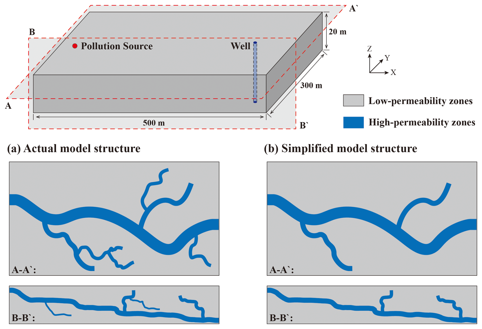
A PCE leakage source is located near the left boundary at the top of the aquifer (x=75 m, y=150 m, z=20 m), with a release rate of 25 kg d⁻¹. During transport, PCE undergoes sequential reductive dechlorination to form trichloroethylene (TCE), dichloroethylene (DCE), and vinyl chloride (VC). A pumping well is located near the right boundary at the bottom of the aquifer (x=475 m, y=150 m, z=7 m) with a pumping rate of 30 m³ d⁻¹, where the concentrations of PCE, TCE, DCE, and VC are continuously monitored.

In practice, detailed structural information of the aquifer is often unavailable, and simplification of the aquifer structure is therefore typically required. In particular, for preferential pathways with hierarchical branching structures, smaller branch channels are often neglected. In this case, only the main preferential pathways are retained (Fig. 2b), and the PCE reactive transport model is constructed based on the simplified aquifer structure. The model is numerically solved using MODFLOW-2005 and RT3D. Gaussian process regression (GPR) is further employed to correct the structural error introduced by simplification of high-permeability preferential pathways.

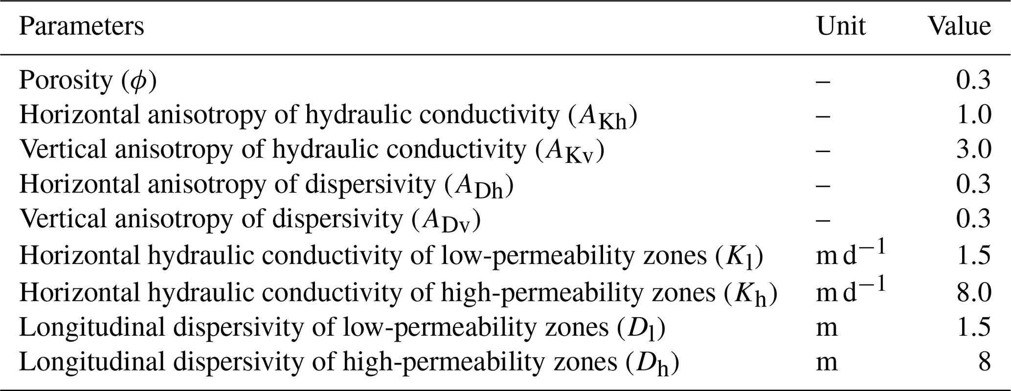
Except for the representation of the preferential pathways, the simplified model is identical to the actual model in all other respects. The total simulation period is 500 d with a time step of 10 d. The parameter settings of the actual model are listed in Table 1. The contaminant concentrations simulated at the pumping well are treated as observational data. Gaussian white noise with a mean of 0 and a variance of 0.01 is added to the simulated concentrations, yielding a total of 50 concentration observations, of which the first 30 are used for parameter identification and the remaining 20 for model validation.

Table 1 Parameter configuration for the synthetic groundwater PCE reactive transport model with the actual model structure.

3.2 Sand Column Cadmium-phosphate Cotransport Model

To investigate the influence of phosphate on cadmium (Cd) transport in natural groundwater environments, a one-dimensional cadmium–phosphate cotransport sand column experiment was conducted (Wu et al., 2022) (Fig. 3). A polypropylene column with a height of 5 cm and an inner diameter of 1.5 cm was used. Stainless steel screens with a pore size of 10 µm were placed at both ends of the column to support the porous medium. The column was uniformly packed with dry soil, and the average porosity (0.4) and bulk density (1.24 g cm⁻³) were determined using the gravimetric method. A peristaltic pump was used to drive the solution upward through the column at a flow rate of 0.2 mL min⁻¹. After complete saturation, the column was flushed with background solution for 12 h, followed by a tracer test to determine flow and solute transport parameters. Once geochemical conditions stabilized, 420 mL of a mixed solution containing 0.1 mM Cd and 1 mM phosphate was injected into the column using the peristaltic pump. After completion of the mixed-solution injection, the influent was switched to background solution without Cd. During the experiment, effluent samples were collected every 90 min using an automatic fraction collector, and Cd concentrations were measured, yielding a total of 58 concentration observations.

Figure 3 Schematic illustration of the sand column Cd-phosphate cotransport experiment.

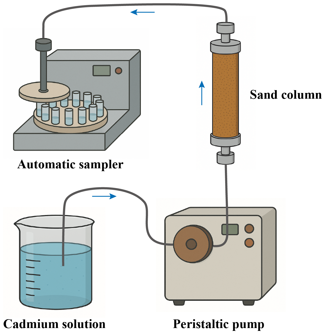
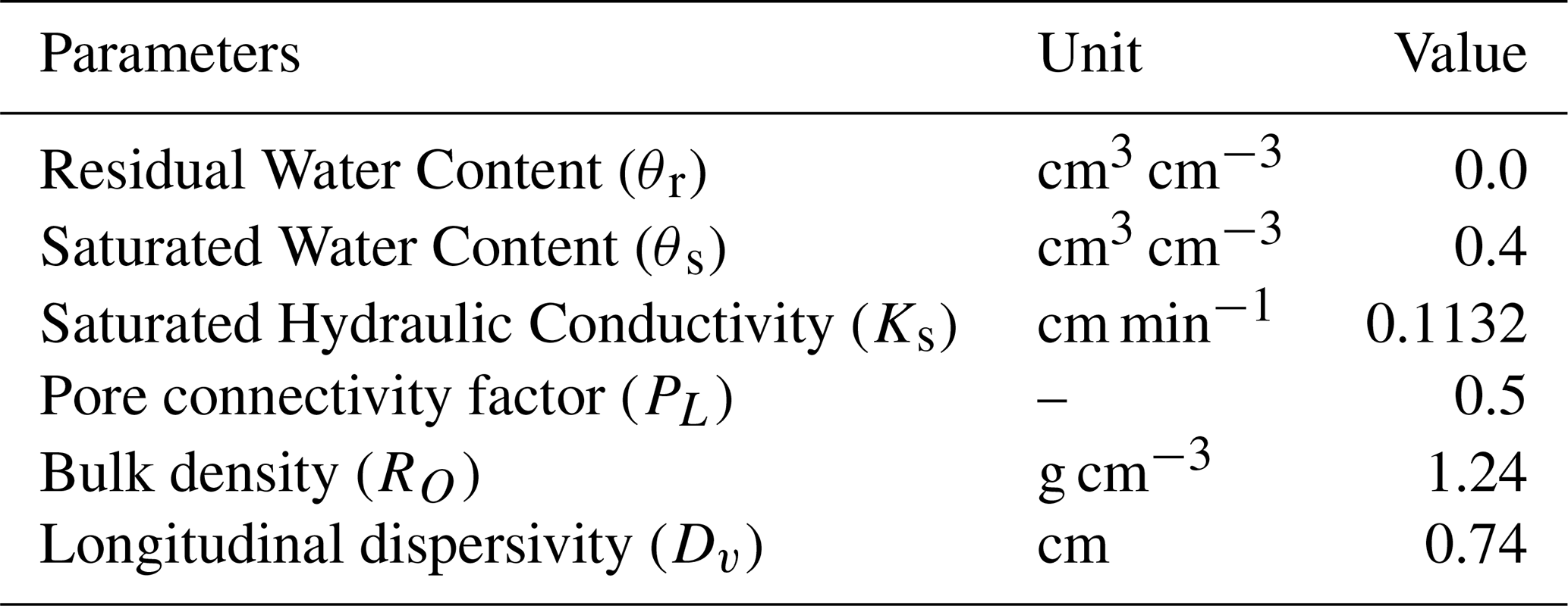
In real-world groundwater contamination scenarios, the spatial distribution of phosphate is often uncertain and its influence on Cd transport is therefore commonly neglected. Accordingly, case study 2 does not account for the cotransport mechanism between Cd and phosphate. A one-dimensional groundwater model for Cd transport was developed using HYDRUS-1D (Nkedikizza et al., 1984; Vangenuchten, 1980), in which a two-site sorption model coupled with a Freundlich isotherm was employed to describe Cd transport. The parameter settings of the physical model are listed in Table 2. In addition, Gaussian process regression (GPR) was employed to correct the structural error arising from neglecting the Cd-phosphate cotransport mechanism. Of the 58 observations, the first 32 were used for parameter identification and the remaining 26 for validation.

Table 2 Parameter configuration of the sand column Cd-phosphate cotransport model.

4 Application of the Methods

In each case study, contaminant transport simulations are first performed using a groundwater model with structural error, after which the model is corrected within the DDM framework. In addition, three scenarios are considered: without physical constraints, with a single physical constraint, and with multiple physical constraints.

4.1 DDM for Synthetic Groundwater PCE Reactive Transport Model

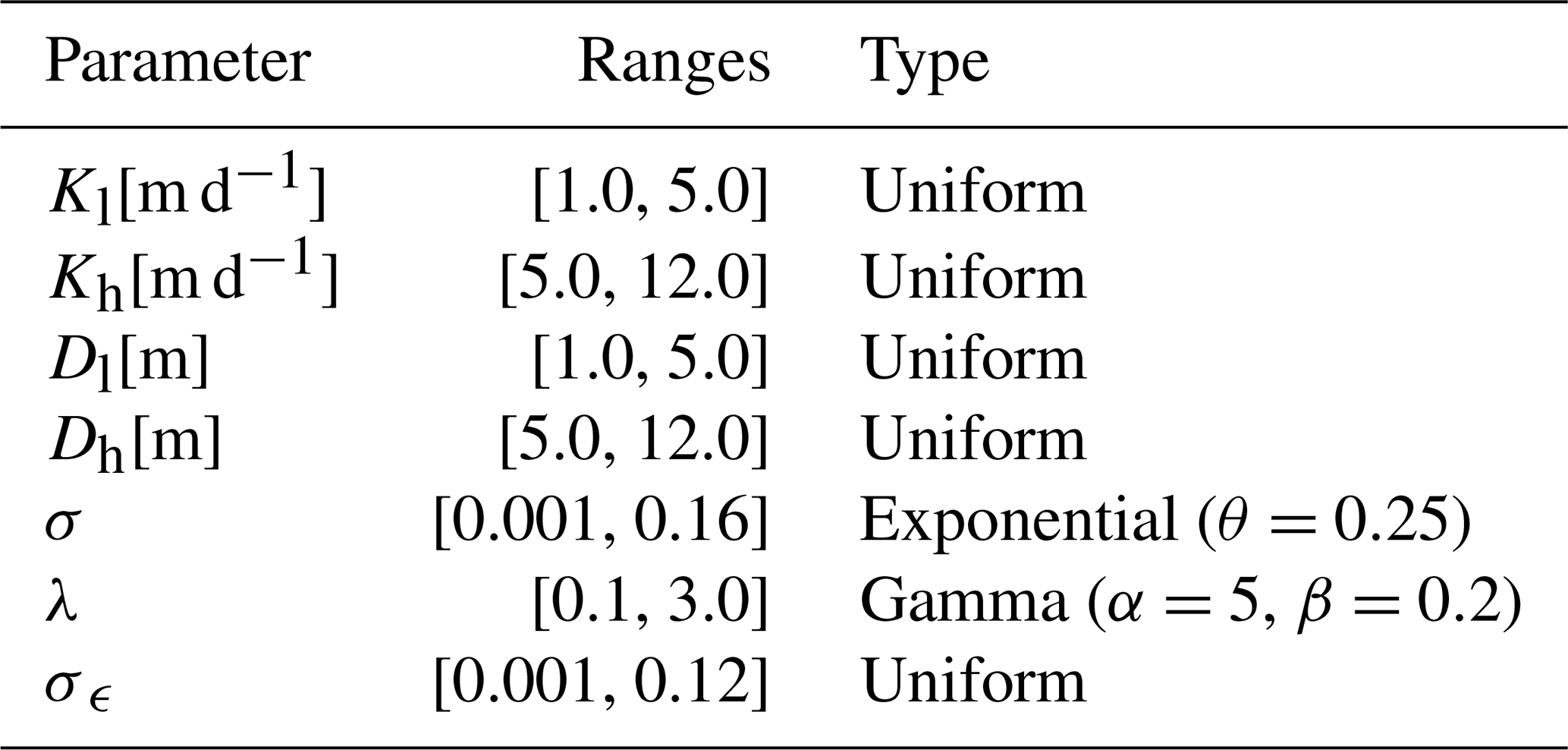
As described in Sect. 3.1, case study 1 constructed a groundwater model with a simplified representation of preferential pathways in the aquifer to simulate PCE reactive transport. In this model, the hydraulic conductivities and dispersivities of the low- and high-permeability zones are treated as random variables with uniform prior distributions. Meanwhile, the GPR hyperparameters σ, λ and σ_ϵ are assigned exponential, gamma, and uniform priors, respectively. Table 3 summarizes the prior information for the physical parameters and the hyperparameters.

Table 3 Prior distributions of parameters for the synthetic groundwater PCE reactive transport model.

In this case study, because carbon and chlorine are the key constituent elements of PCE and its dechlorination products, carbon and chlorine mass conservation constraints are incorporated into the DDM. Under the single-constraint scenario, only the carbon mass conservation constraint is coupled, whereas under the multiple-constraint scenario both carbon and chlorine mass conservation constraints are coupled simultaneously. For the entire system, the total mass of leaked carbon/chlorine is equal to the total carbon/chlorine mass contained in PCE, TCE, DCE, and VC. Moreover, at any time, the total mass of leaked carbon/chlorine m_l should equal the sum of three components: the mass remaining in the aquifer m_r, the mass leaving the aquifer through its boundaries m_b, and the mass extracted by the pumping well m_w. The mass balance error is defined as M_error, and the corresponding mass conservation constraints for carbon/chlorine can be expressed as:

$$\begin{array}{}\text{(24)}& M_{\mathrm{error}}=m_{\mathrm{l}}-(m_{\mathrm{r}}+m_{\mathrm{b}}+m_{\mathrm{w}})=\mathrm{0}\end{array}$$

Since the observation intervals are much larger than the simulation time step of the physical model, the physical constraints at different observation times are assumed to be independent and enforced with equal strength. The confidence on the accuracy of each physical constraint (${\mathit{\sigma }}_{c,i}^{\mathrm{2}}$) is set to 0.2 (sensitivity analysis shown in Fig. S1 in the Supplement). Accordingly, the likelihood function associated with the carbon/chlorine mass conservation constraints can be expressed as:

$$\begin{array}{}\text{(25)}& \begin{array}{rl}& p(M_{\mathrm{error}}=\mathrm{0}\left|\mathit{\theta },\mathit{\phi }\right.)={\displaystyle \frac{\mathrm{1}}{\sqrt{(\mathrm{2}\mathit{\pi }{)}^n\left|{\sum }_c\right|}}}\\ & \exp \left(-{\displaystyle \frac{\mathrm{1}}{\mathrm{2}}}[m_{\mathrm{l}}-(m_{\mathrm{r}}+m_{\mathrm{b}}+m_{\mathrm{w}}){]}^T\right.\\ & \left.\sum _c^{-\mathrm{1}}\left[m_{\mathrm{l}}-(m_{\mathrm{r}}+m_{\mathrm{b}}+m_{\mathrm{w}})\right]\right)\end{array}\end{array}$$

In addition, following Kadhar and Baskar (2018), the sliding window length used for dynamic weight updating is set to γ=10, and the minimum tolerance variance is set to Tol${}_{\mathrm{fun}}={\mathrm{10}}^{-\mathrm{4}}$. The dynamic sub-likelihood weight-updating strategy with a stopping criterion is implemented as described in Sect. 2.3. Three scenarios are considered: without physical constraints, with only the carbon mass conservation constraint, and with both carbon and chlorine mass conservation constraints.

After specifying the prior distributions and constructing the combined likelihood function, MCMC simulations were conducted to infer the posterior distributions of the parameters. Both unconstrained and constrained DDM configurations use the same MCMC settings based on the DREAMzs algorithm, with three parallel Markov chains, each running for 9000 iterations, and the first 6000 iterations designated as burn-in. Finally, based on the identified posterior parameter distributions, the predictive performance of the DDM for the concentrations of the four chlorinated hydrocarbons was evaluated under the three scenarios.

4.2 DDM for Sand Column Cd-phosphate Cotransport Model

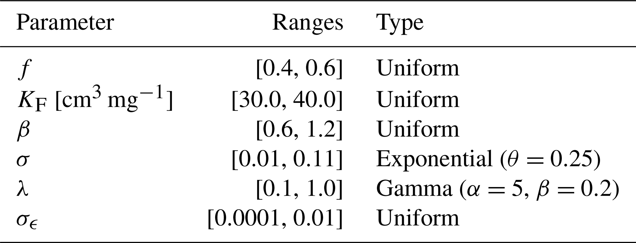
As described in Sect. 3.2, case study 2 developed a simplified Cd transport model that does not consider the cadmium-phosphate cotransport mechanism. The proportion coefficient of equilibrium sorption f, the Freundlich isotherm coefficient K_F, and the isotherm shape parameter β of the physical model are treated as random variables with uniform prior distributions. The GPR hyperparameters σ, λ and σ_ϵ are assigned exponential, gamma, and uniform prior distributions, respectively. The prior information for the physical model parameters and the GPR hyperparameters is summarized in Table 4.

Table 4 Prior distributions of parameters for the sand column Cd-phosphate cotransport model.

In this case study, Cd mass conservation and Cd concentration bound constraints are incorporated into the DDM. Under the single-constraint scenario, only the Cd mass conservation constraint is coupled. At any given time t_i, the total mass of Cd entering the column is assumed to be equal to the sum of the Cd masses present in different states. Specifically, before Cd breakthrough (t_i≤t₀), the total mass consists of the dissolved-phase mass m_d and the mass adsorbed onto the solid phase m_a. After breakthrough (t_i>t₀), the total mass additionally includes the Cd mass in the effluent, m_out. Accordingly, the Cd mass conservation constraint is defined as:

$$\begin{array}{}\text{(26)}& M_{\mathrm{error},{\mathrm{t}}_i}=\left\{\begin{array}{ll}{m}_{\mathrm{in},{\mathrm{t}}_i}-(m_{\mathrm{d},{\mathrm{t}}_i}+m_{\mathrm{a},{\mathrm{t}}_i})=\mathrm{0},& t_i\le t_{\mathrm{0}}\\ m_{\mathrm{in},{\mathrm{t}}_i}-(m_{\mathrm{d},{\mathrm{t}}_i}+m_{\mathrm{a},{\mathrm{t}}_i}+m_{\mathrm{out},{\mathrm{t}}_i})=\mathrm{0},& t_i\le t_{\mathrm{0}}\end{array}\right.\end{array}$$

where $m_{\mathrm{in},{\mathrm{t}}_i}$ denotes the total Cd mass entering the column; $m_{\mathrm{d},{\mathrm{t}}_i}$, $m_{\mathrm{a},{\mathrm{t}}_i}$ and $m_{\mathrm{out},{\mathrm{t}}_i}$ denote the Cd mass in the dissolved phase, sorbed phase, and effluent, respectively; and t₀ represents the time of first Cd breakthrough.

Consistent with case study 1, the confidence on the accuracy of each physical constraint (${\mathit{\sigma }}_{c,i}^{\mathrm{2}}$) is set to 0.2 (sensitivity analysis shown in Supplement Fig. S2), and the corresponding likelihood function can be written as:

$$\begin{array}{}\text{(27)}& \begin{array}{rl}& p(M_{\mathrm{error}}=\mathrm{0}\left|\mathit{\theta },\mathit{\phi }\right.)\\ & =\left\{\begin{array}{l}\begin{array}{rl}& {\displaystyle \frac{\mathrm{1}}{\sqrt{(\mathrm{2}\mathit{\pi }{)}^{n_{\mathrm{0}}}\left|{\sum }_c\right|}}}\exp \left(-{\displaystyle \frac{\mathrm{1}}{\mathrm{2}}}[m_{\mathrm{in}}-(m_{\mathrm{d}}+m_{\mathrm{a}}){]}^T\right.\\ & \left.\sum _c^{-\mathrm{1}}[m_{\mathrm{in}}-(m_{\mathrm{d}}+m_{\mathrm{a}}\left)\right]\right)\end{array}\\ \begin{array}{rl}& {\displaystyle \frac{\mathrm{1}}{\sqrt{(\mathrm{2}\mathit{\pi }{)}^{(n-n_{\mathrm{0}})}\left|{\sum }_c\right|}}}\exp \left(-{\displaystyle \frac{\mathrm{1}}{\mathrm{2}}}[m_{\mathrm{in}}-(m_{\mathrm{d}}+m_{\mathrm{a}}+m_{\mathrm{out}}){]}^T\right.\\ & \left.\sum _c^{-\mathrm{1}}[m_{\mathrm{in}}-(m_{\mathrm{d}}+m_{\mathrm{a}}+m_{\mathrm{out}}\left)\right]\right)\end{array}\end{array}\right.\end{array}\end{array}$$

where n is the total number of observations and n₀ is the number of observations before Cd breakthrough.

Under the multiple-constraint scenario, the Cd concentration bound constraint is further coupled. The experimental breakthrough curve indicates that the upper bound of Cd concentration does not exceed 75 % of the initial influent concentration C₀. Therefore, the Cd concentration bound constraint is defined as:

$$\begin{array}{}\text{(28)}& \mathrm{0}\le {\displaystyle \frac{C_{\mathrm{Cd}}}{C_{\mathrm{0}}}}\le \mathrm{0.75}\end{array}$$

This constraint is transformed into an equivalent equality constraint and assumed to follow a Gaussian distribution $N(\mathrm{0},{\sum }_f)$, which can be expressed as:

$$\begin{array}{}\text{(29)}& Z\left(y\right)=\left[max\left(\mathrm{0},-{\displaystyle \frac{C_{\mathrm{Cd}}}{C_{\mathrm{0}}}}\right)+max\left(\mathrm{0},{\displaystyle \frac{C_{\mathrm{Cd}}}{C_{\mathrm{0}}}}-\mathrm{0.75}\right)\right]=\mathrm{0}\end{array}$$

Accordingly, the likelihood function associated with the Cd concentration bound constraint can be expressed as:

$$\begin{array}{}\text{(30)}& \begin{array}{rl}p\left(Z\right(y)=& \mathrm{0}\left|\mathit{\theta },\mathit{\phi }\right.)={\displaystyle \frac{\mathrm{1}}{\sqrt{(\mathrm{2}\mathit{\pi }{)}^n\left|{\sum }_f\right|}}}\\ & \exp \left(-{\displaystyle \frac{\mathrm{1}}{\mathrm{2}}}{\left[Z\left(y\right)=\mathrm{0}\right]}^T\sum _c^{-\mathrm{1}}\left[Z\left(y\right)=\mathrm{0}\right]\right)\end{array}\end{array}$$

As in case study 1, the sliding window length (γ=10) and minimum tolerance variance (Tol${}_{\mathrm{fun}}={\mathrm{10}}^{-\mathrm{4}}$) are used for dynamic sub-likelihood weight updating and the stopping criterion. As in case study 1, three scenarios are considered: without physical constraints, with only the Cd mass conservation constraint, and with both the Cd mass conservation and Cd concentration bound constraints.

MCMC simulations were then conducted to infer the posterior distributions of the parameters. Under all three scenarios, identical MCMC settings based on the DREAMzs algorithm are employed, with three parallel Markov chains, each running for 9000 iterations and the first 6000 iterations designated as burn-in. Based on the identified posterior parameter distributions, the predictive performance of the DDM for Cd concentrations is evaluated under the three scenarios.

5 Results and Discussions

5.1 Parameter Estimations

5.1.1 Synthetic Groundwater PCE Reactive Transport Model

Figure 4 presents the posterior distributions of the PCE reactive transport model parameters under the three scenarios, where the first row shows the physical model parameters and the second row showing the GPR hyperparameters. The results indicate that both the presence and the number of coupled physical constraints significantly influence the posterior distributions. Under the unconstrained and single-constraint scenarios, the posterior distributions are generally similar, exhibiting relatively wide ranges and lower peak probability densities, indicating greater parameter uncertainty. In contrast, when multiple physical constraints are coupled simultaneously, the posterior distributions contract substantially. Specifically, the posterior ranges become substantially narrower and the peak densities increase markedly. Notably, the posterior distributions of the physical model parameter K_l and the GPR hyperparameters σ, λ and σ_ϵ show particularly pronounced changes in terms of range, mean value, and peak density (Fig. 4a and e–g). In addition, the physical model parameters K_h, L_l and L_h exhibit more pronounced multimodal characteristics (Fig. 4b–d), suggesting the presence of multiple plausible parameter combinations.

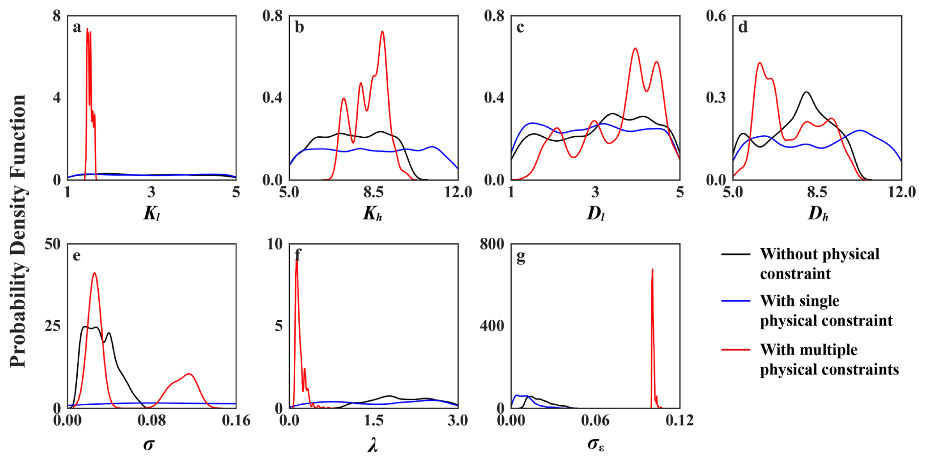
Figure 4 Parameter posterior distributions for the synthetic groundwater PCE reactive transport model under the three scenarios.

5.1.2 Sand Column Cd-phosphate Cotransport Model

Figure 5 presents the posterior distributions of the parameters of the Cd-phosphate cotransport model under the three scenarios, where the first and second rows correspond to the physical model parameters and the GPR hyperparameters, respectively. Under the unconstrained and single-constraint scenarios, most parameters exhibit wide posterior ranges and low peak probability densities, indicating greater parameter uncertainty. Except for the relatively flat probability density curves for the physical model parameter K_F and the GPR hyperparameter λ (Fig. 5b and e), the posterior distributions of the remaining parameters display varying degrees of multimodality. In contrast, when multiple physical constraints are simultaneously coupled, the posterior distributions of all parameters exhibit substantial contraction and markedly higher peak densities. Among them, the changes are particularly pronounced for the physical model parameter K_F and the GPR hyperparameters σ and λ (Fig. 5b and d–e).

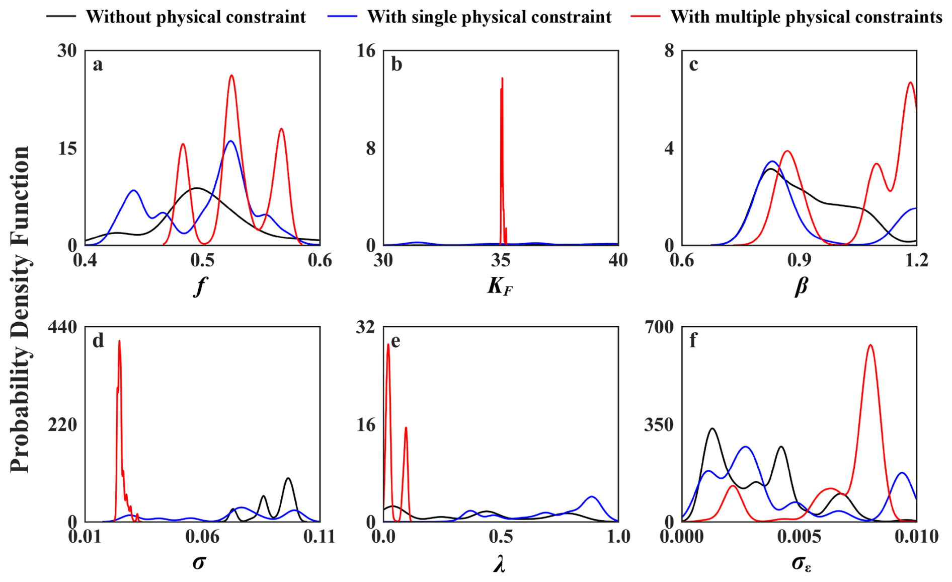
Figure 5 Parameter posterior distributions for the sand column Cd–phosphate cotransport model under the three scenarios.

5.2 Mass Conservation Evaluation

5.2.1 Synthetic Groundwater PCE Reactive Transport Model

Figure 6 illustrates the temporal variation in the carbon and chlorine mass balance error rates (ERs) predicted by the DDM under the three scenarios for case study 1. During the simulation, the contamination source continuously releases PCE at a rate of 25 kg d⁻¹, containing 3.63 kg of carbon and 21.37 kg of chlorine. The mass balance error rate (ER) for $\mathrm{carbon}/\mathrm{chlorine}$ is defined as:

$$\begin{array}{}\text{(31)}& \mathrm{ER}={\displaystyle \frac{M_{\mathrm{T}}-M_{\mathrm{S}}}{M_{\mathrm{T}}}}\times \mathrm{100}\mathit{\%}\end{array}$$

where M_T and M_S denote the true total mass of $\mathrm{carbon}/\mathrm{chlorine}$ in the system and the corresponding total mass predicted by the DDM, respectively.

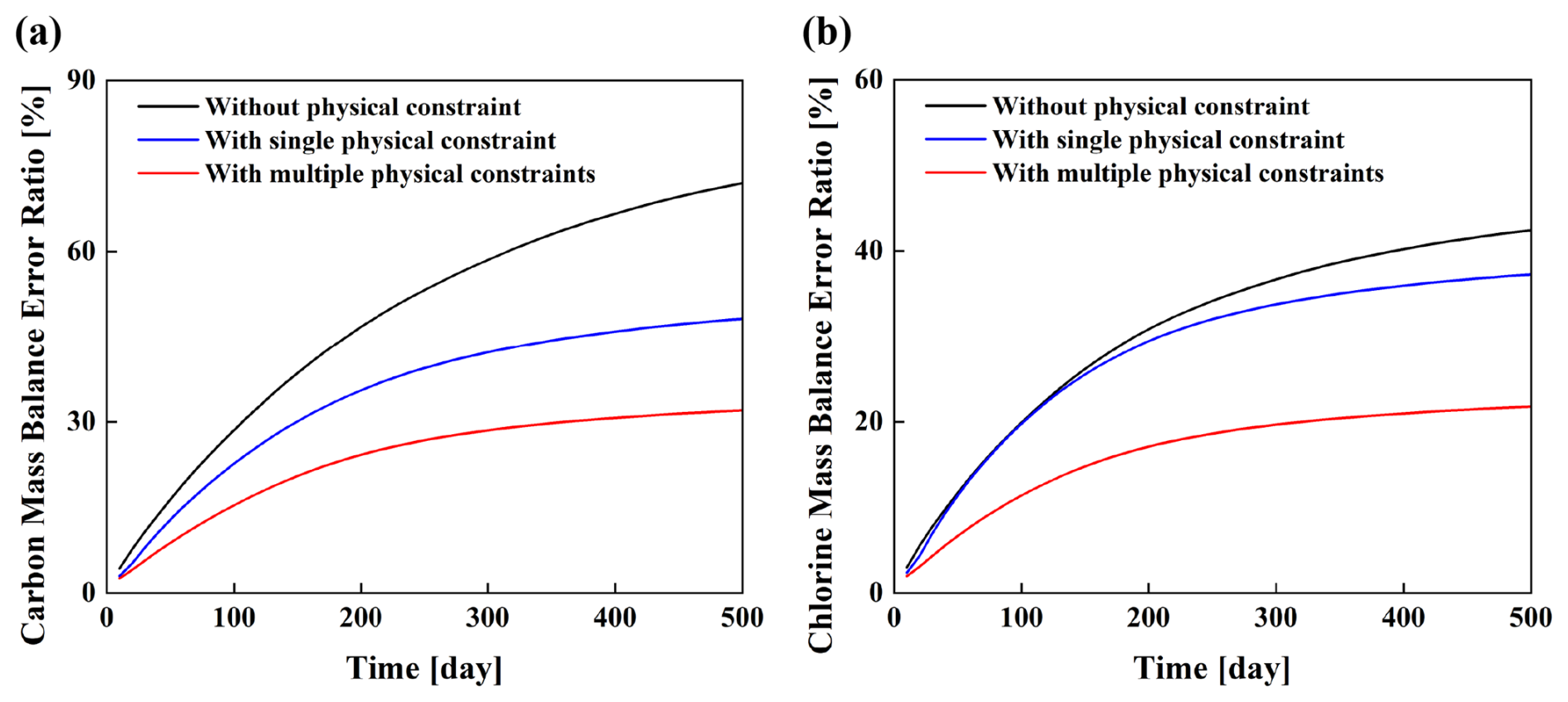
Figure 6 Variation in the $\mathrm{carbon}/\mathrm{chlorine}$ mass balance error rate for the synthetic groundwater PCE reactive transport model under the three scenarios.

The results indicate that coupling physical constraints significantly reduces the mass conservation error of the DDM predictions. Under the unconstrained scenario, the mean mass conservation ERs for carbon and chlorine reach 48.62 % and 30.65 %, corresponding to average mass errors of 1.76 and 6.55 kg, respectively. After coupling the carbon mass conservation constraint, the mean ER for carbon decreases to 35.03 %, with the average mass error reduced to 1.27 kg. Meanwhile, the mean ER for chlorine decreases slightly to 28.27 %, with an average mass error of 6.04 kg. When both carbon and chlorine mass conservation constraints are simultaneously coupled, the mean ERs for carbon and chlorine further decrease to 23.63 % and 16.49 %, with the corresponding average mass errors reduced to 0.86 and 3.52 kg, respectively. Moreover, compared with the unconstrained scenario, coupling physical constraints results in a more gradual increase in the $\mathrm{carbon}/\mathrm{chlorine}$ ER over time, followed by stabilization in the later stages of the simulation.

5.2.2 Sand Column Cd-phosphate Cotransport Model

Figure 7 presents the temporal variation of the Cd mass conservation error rate (ER) predicted by the DDM under the three scenarios in case study 2. Over the entire experiment period, a total of 4.72 mg of Cd is introduced into the soil column. Under the unconstrained scenario, the mean mass conservation ER for Cd is 30.14 %, with an average mass error of 1.42 mg. The peak ER reaches 57.14 %, corresponding to a maximum mass error of 2.70 mg. When only the Cd mass conservation constraint is coupled, the mean and peak ERs decrease markedly to 13.64 % and 26.07 %, respectively, with the corresponding average and maximum mass errors substantially reduced to 0.64 and 1.23 mg. When both the Cd mass conservation and concentration bound constraints are simultaneously coupled, the mean and peak ERs further decrease to 10.36 % and 19.33 %, respectively, with the corresponding average and maximum mass errors reduced to 0.49 and 0.91 mg.

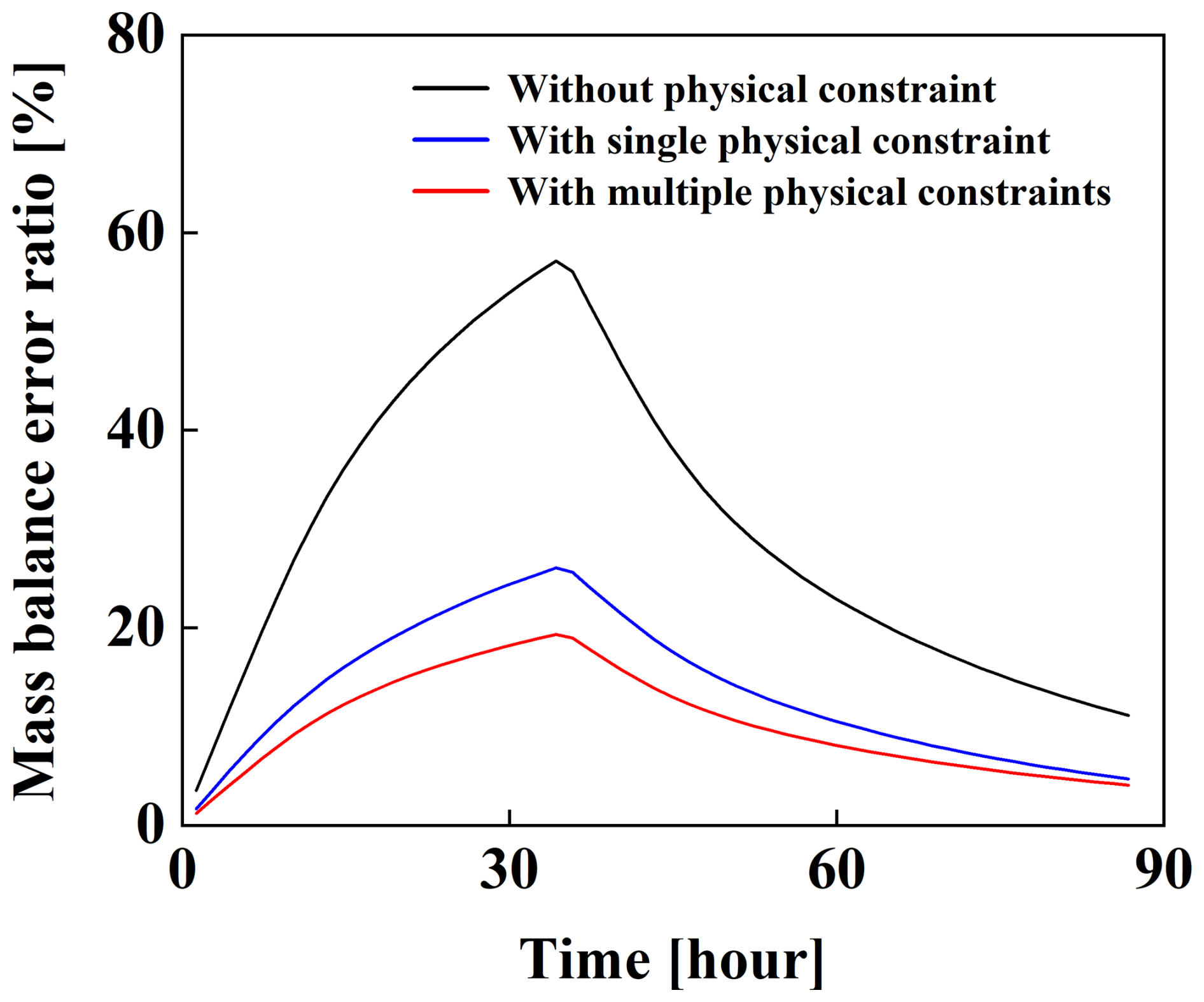
Figure 7 Variation in the cadmium mass balance error rate for the sand column Cd-phosphate cotransport model under the three scenarios.

5.3 Prediction Performance

5.3.1 Synthetic Groundwater PCE Reactive Transport Model

Figure 8 presents the temporal variations in concentrations of four chlorinated hydrocarbons predicted by the DDM under the three scenarios in case study 1. Under the unconstrained scenario, the model captures the overall trends of chlorinated hydrocarbon concentrations. However, noticeable discrepancies remain between the posterior means and the observations during the validation period (Fig. 8a–d), particularly for DCE and VC (Fig. 8c and d). After coupling a single physical constraint, the DDM shows improved predictive performance. The predicted TCE concentrations become closer to the observations, whereas substantial deviations from the observations remain for the other chlorinated hydrocarbons during the validation period. In contrast, when multiple physical constraints are simultaneously coupled, the predictive accuracy for all four chlorinated hydrocarbons improves markedly, with particularly pronounced improvements during the validation period (Fig. 8i–l).

Figure 8 DDM predictions of chlorinated ethenes concentrations under the three scenarios.

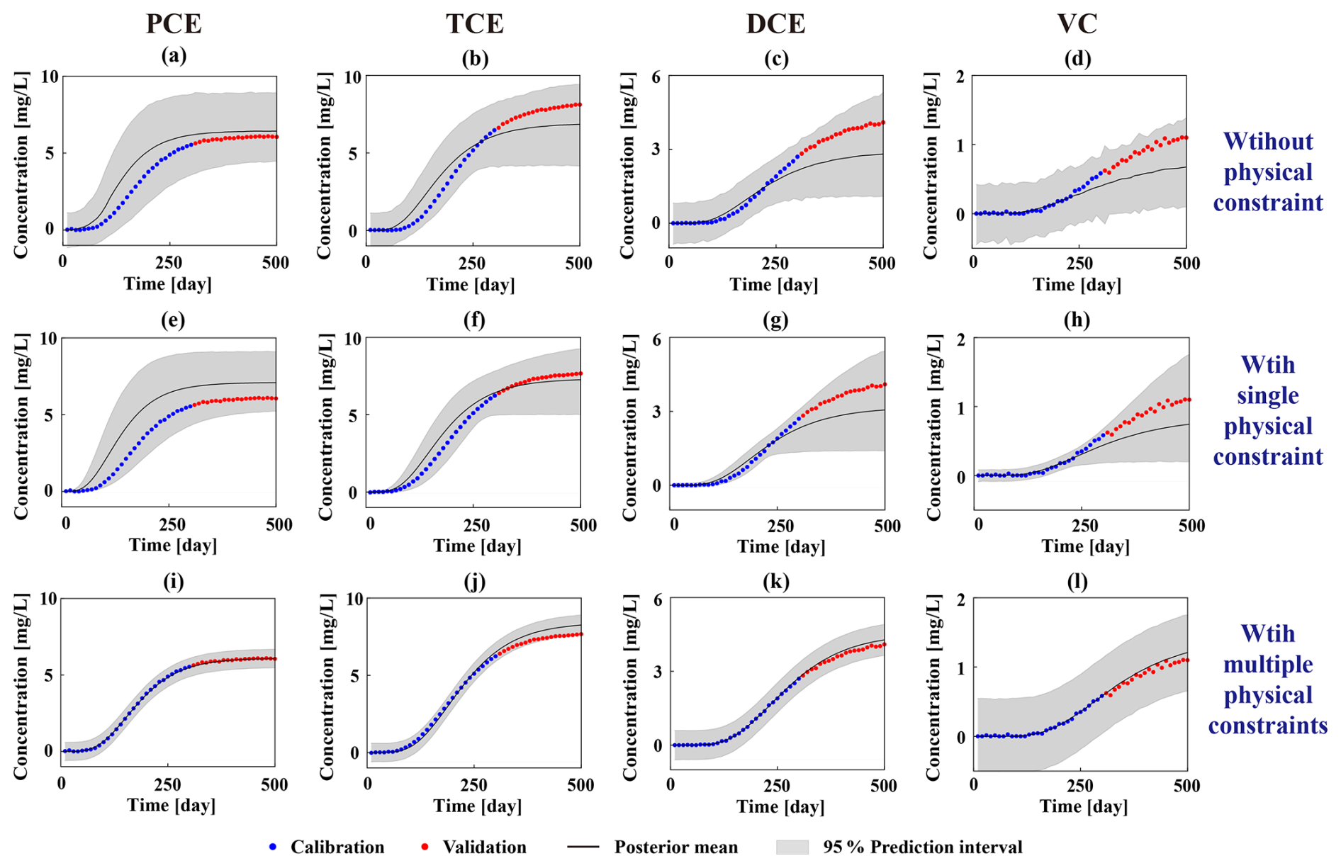
Moreover, under the unconstrained scenario, the 95 % prediction intervals are generally wider, especially during the validation period (Fig. 8a–d). When a single physical constraint is coupled, the predictive intervals narrow during the calibration period but remain wide during the validation period, particularly for DCE and VC (Fig. 8g and h). In contrast, simultaneously coupling multiple physical constraints markedly reduces the prediction intervals for all chlorinated hydrocarbons (Fig. 8i–l), and the corresponding average widths of the 95 % prediction intervals are substantially smaller (Table S1), indicating a substantial reduction in predictive uncertainty.

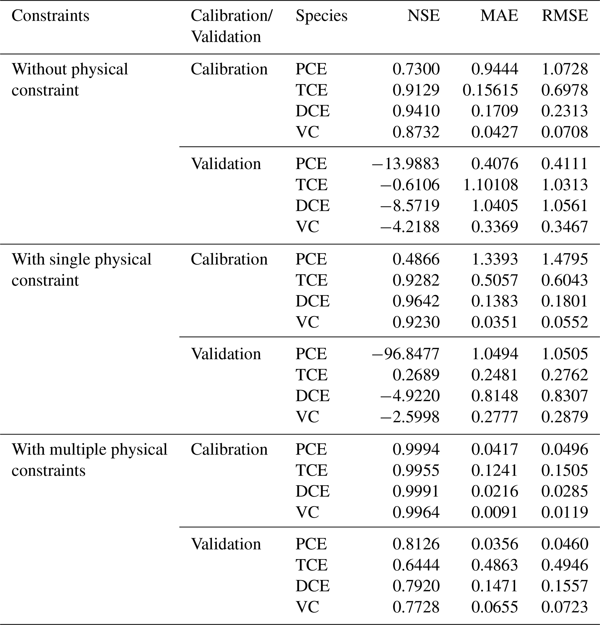
Table 5 summarizes the quantitative evaluation of DDM predictive performance under the three scenarios in case study 1. Compared with the unconstrained scenario, coupling a single physical constraint leads to a modest improvement in the NSE of the predicted concentrations for the four chlorinated hydrocarbons during the validation period, although the improvement remains limited. Except for PCE, for which MAE and RMSE increase slightly, MAE and RMSE decrease for the other chlorinated hydrocarbons. Specifically, the MAE and RMSE of TCE decrease by 77.47 % and 73.22 %, respectively, whereas those of DCE and VC decrease by only about 20 %. When multiple physical constraints are coupled, the predictive performance of the DDM improves markedly relative to the single-constraint scenario. During the validation period, TCE behaves differently from the other chlorinated hydrocarbons: its NSE increases from 0.2689 to 0.6444 (approximately 139.64 %), whereas its MAE and RMSE increase slightly. In contrast, the NSE values of the other chlorinated hydrocarbons increase markedly from negative values to approximately 0.8, accompanied by substantial reductions in MAE and RMSE. Specifically, both MAE and RMSE decrease by approximately 95 % for PCE, 81 % for DCE, and 75 % for VC.

Table 5 Evaluation of predictions for the synthetic groundwater PCE reactive transport model under the three scenarios.

5.3.2 Sand Column Cd-phosphate Cotransport Model

Figure 9 presents the temporal variation in Cd concentration predicted by the DDM under the three scenarios in case study 2. Under the unconstrained scenario, the model captures the overall trend of Cd concentration, which first increases and then decreases. However, noticeable discrepancies remain between the posterior means and the observations, with the concentration peak overestimated and concentrations during the validation period markedly underestimated (Fig. 9a). After coupling the Cd mass conservation constraint, the DDM predictions become more consistent with the observations. Except for residual deviations at the early and late stages of the simulation, the posterior mean aligns more closely with the observations at most time points (Fig. 9b). When multiple physical constraints are simultaneously coupled, the predictive accuracy of the DDM improves markedly, with particularly evident improvements at the concentration peak and during the validation period (Fig. 9c).

Figure 9 DDM predictions of cadmium concentration under the three scenarios.

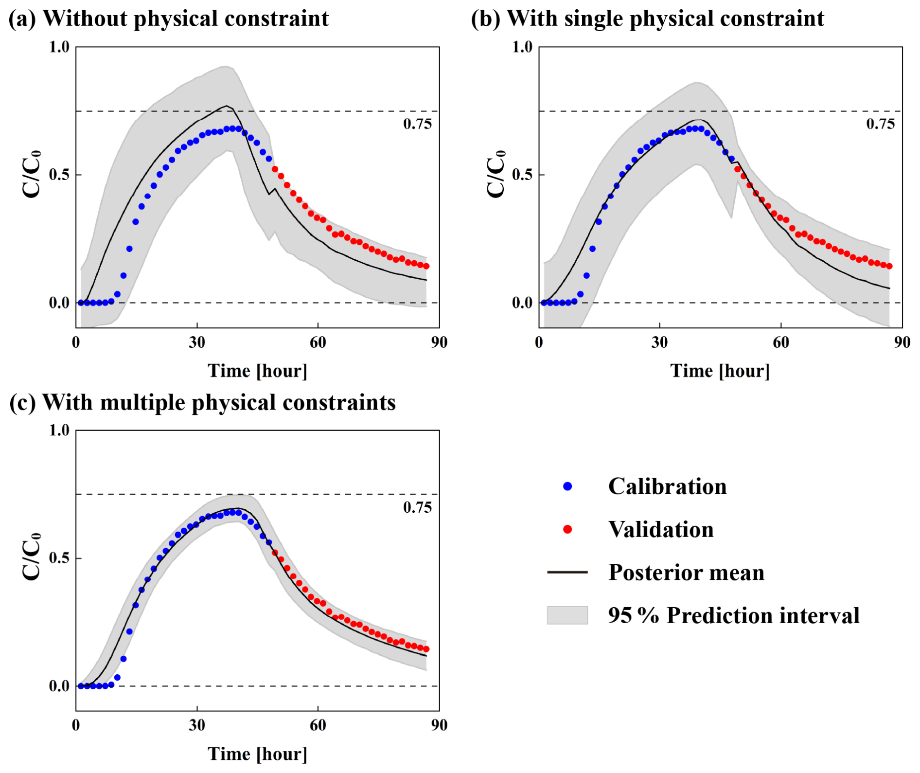
In addition, predictive uncertainty differs substantially among the scenarios. Under the unconstrained scenario, the 95 % prediction intervals are relatively wide (Fig. 9a). After coupling a single physical constraint, the width of the prediction intervals changes only marginally. Notably, some posterior predictions still fall outside the physically plausible range of Cd concentration, with the predicted maximum exceeding the highest observed value and the predicted minimum concentration dropping below zero (Fig. 9b). In contrast, when the Cd concentration bound constraint is additionally coupled, all posterior predictions remain within the physically admissible range, and the corresponding 95 % prediction intervals exhibit substantially smaller average widths (Table S2), indicating a marked reduction in predictive uncertainty.

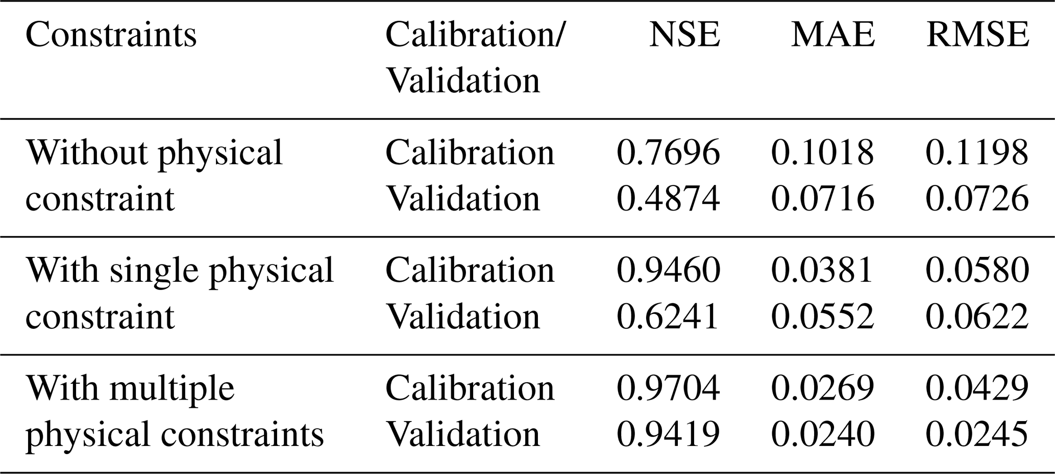
Table 6 presents the quantitative evaluation of the DDM predictive performance under the three scenarios in case study 2. Compared with the unconstrained scenario, coupling a single physical constraint increases the NSE of Cd concentration predictions during the validation period from 0.4874 to 0.6241 (an improvement of approximately 28.05 %), while the MAE and RMSE decrease by approximately 22.91 % and 14.33 %, respectively. When multiple physical constraints are simultaneously coupled, the NSE during the validation period further increases from 0.6241 to 0.9419 (an improvement of approximately 50.92 %) relative to the single-constraint scenario, while the MAE and RMSE decrease by approximately 56.52 % and 60.61 %, respectively, indicating a substantial improvement in predictive performance.

Table 6 Evaluation of predictions for the sand column Cd-phosphate cotransport model under the three scenarios.

5.4 Discussions

5.4.1 Updating of Sub-likelihood Function Weights

Since sub-likelihood functions associated with different physical constraints represent distinct physical mechanisms, their numerical scales often differ by several orders of magnitude. In case study 1, sub-likelihood values differ by up to six orders of magnitude, whereas in case study 2 they differ by approximately one order of magnitude. Such scale disparities cause smaller sub-likelihoods to be overshadowed by larger ones during parameter identification, thereby diminishing the influence of certain physical constraints in Bayesian inference and making it difficult for the corrected predictions to simultaneously satisfy all constraints. Therefore, dynamically updating sub-likelihood weights in the combined likelihood function is essential to ensure appropriate contributions from each sub-likelihood during parameter identification.

In both case studies, the evolution of sub-likelihood weights over the MCMC iterations indicates that the proposed dynamic weight-updating strategy with a stopping criterion plays a critical role in Bayesian inference (Figs. 10 and 11). After substantial adaptive adjustment in the early iterations, the weights rapidly converge to stable values, effectively rescaling sub-likelihoods that initially differed by several orders of magnitude to a comparable scale. This ensures that all sub-likelihoods exert meaningful influence on parameter identification while avoiding the subjectivity inherent in manually assigned weights. Notably, the stable weighting patterns obtained in the two case studies differ markedly, suggesting that fixed weights are unlikely to be suitable across varying scenarios. In contrast, the proposed dynamic weight-updating strategy is well suited to combined likelihood functions that integrate multiple sub-likelihoods associated with distinct physical mechanisms, resulting in substantially improved predictive accuracy and physical consistency compared with the fixed weighting strategy (Figs. S3–S6, Tables S3 and S4). The proposed strategy maintains a balance between multiple physical constraints and observational information, thereby enhancing the robustness of parameter identification and the effective enforcement of physical constraints. However, the dynamic weight-updating strategy introduces additional computational overhead. Compared with the DDM without physical constraints or with fixed weights, the proposed method requires the weights of sub-likelihood functions to be dynamically calculated and updated during MCMC sampling, with the computational burden increases as more physical constraints are introduced.

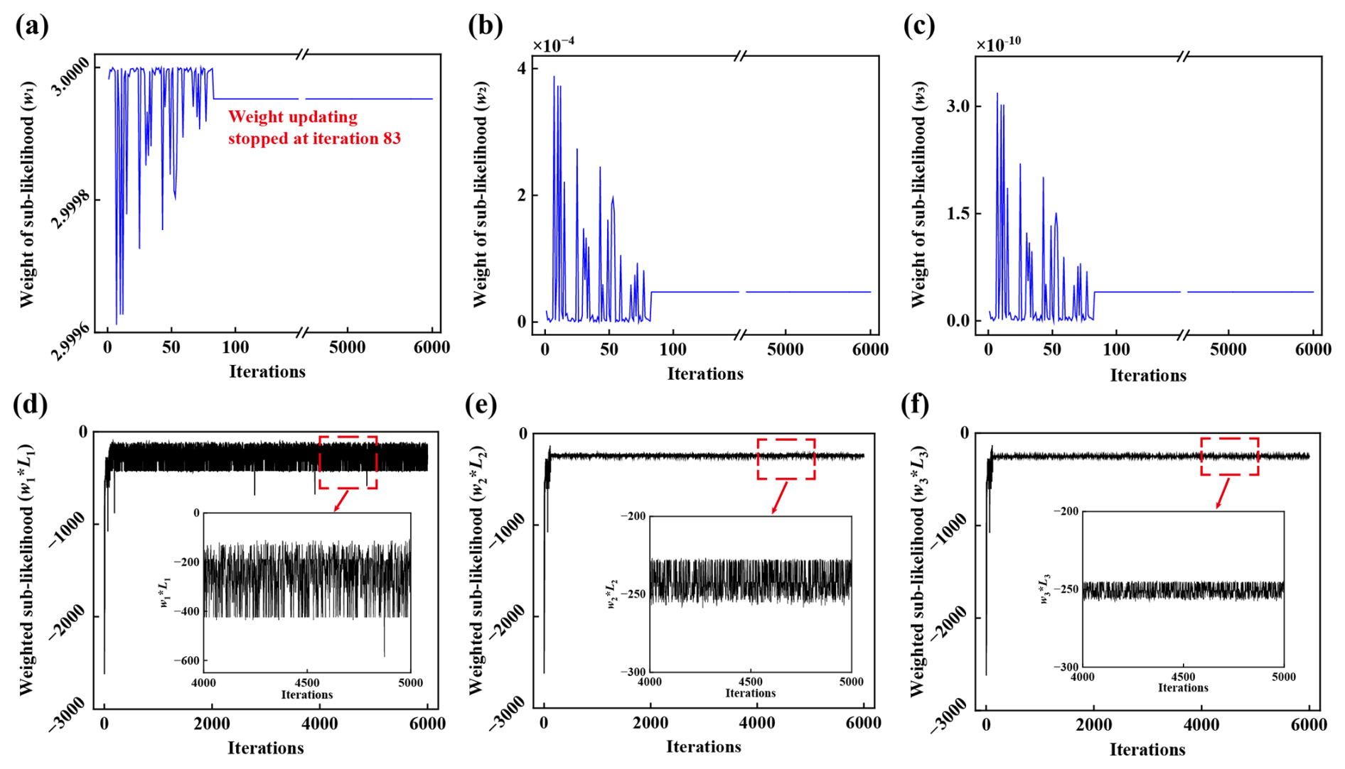
Figure 10 Dynamic updating of sub-likelihood weights (a–c) and weighted sub-likelihoods (d–f) for the synthetic groundwater PCE reactive transport model.

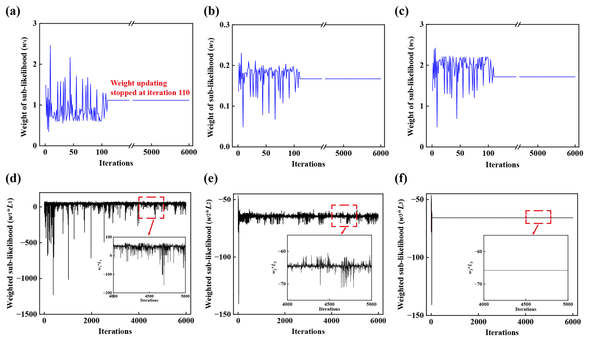
Figure 11 Dynamic updating of sub-likelihood weights (a–c) and weighted sub-likelihoods (d–f) for the sand column Cd-phosphate cotransport model.

5.4.2 Impact of Physical Constraints on Posterior Model Parameters and Predictions

The presence and the number of coupled physical constraints significantly influence the posterior distributions of DDM parameters (Figs. 4 and 5). Without physical constraints, the structural error correction process lacks the constraints imposed by physical mechanisms, causing both the physical model parameters θ and the GPR hyperparameters φ to be excessively adjusted in order to maximize agreement with observations. Although coupling a single physical constraint can partially alleviate this over-adjustment, it is generally insufficient to effectively constrain all parameters. When multiple physical constraints are simultaneously coupled, the posterior distributions of all parameters are confined to physically consistent ranges, thereby effectively mitigating parameter overfitting.

The GPR hyperparameters exhibit greater sensitivity to physical constraints because GPR lacks inherent physical regulation, whereas the parameters of the physical model (groundwater model) are already subject to internal constraints such as mass conservation. Consequently, the hyperparameters are more prone to excessive adjustment than the physical model parameters. The DDM coupled with multiple physical constraints primarily constrains the identification of GPR hyperparameters, leading to substantially more concentrated posterior distributions and effectively reducing parameter uncertainty.

Notably, the observational data available for parameter identification are limited in both case studies, with only 50 and 58 observations in case studies 1 and 2, respectively. Under limited data availability and structural bias in the physical model, parameter identification is subject to substantial uncertainty, resulting in pronounced equifinality. In this context, incorporating appropriate physical constraints effectively restricts the parameter identification process. Within the Bayesian uncertainty analysis, these physical constraints provide additional information for parameter identification, thereby further reducing parameter uncertainty.

The analysis of mass balance errors (Figs. 6 and 7) highlights the necessity of coupling multiple physical constraints during structural error correction. In case study 1, when only the carbon mass conservation constraint is coupled, the mass balance error rate (ER) of chlorine remains at a relatively high level, whereas coupling both carbon and chlorine mass conservation constraints substantially reduces the ERs of both components. In case study 2, although the Cd mass conservation constraint reduces the ER for Cd, the ER decreases further after the concentration bound constraint is additionally coupled. These results indicate that a single physical constraint typically regulates only the predicted variables directly associated with it, whereas predictions of unconstrained variables may still violate physical principles. In contrast, coupling multiple physical constraints constrains the structural error correction process at the level of distinct physical mechanisms, thereby enhancing the physical consistency of DDM predictions.

The presence and the number of coupled physical constraints also significantly influence the forms of structural error (Figs. 12 and 13). Without physical constraints, structural errors exhibit large amplitudes and greater complexity, making them difficult for the GPR model to characterize accurately. Coupling a single physical constraint partially suppresses the amplitude of structural error variations. In contrast, when multiple physical constraints are coupled simultaneously, the posterior distributions of model parameters are further constrained, leading to substantially smaller and more stable structural error fluctuations, characterized by smaller standard deviation and range (Tables S5 and S6). As a result, the complexity of structural error is markedly reduced, enabling the GPR model to predict structural errors more accurately.

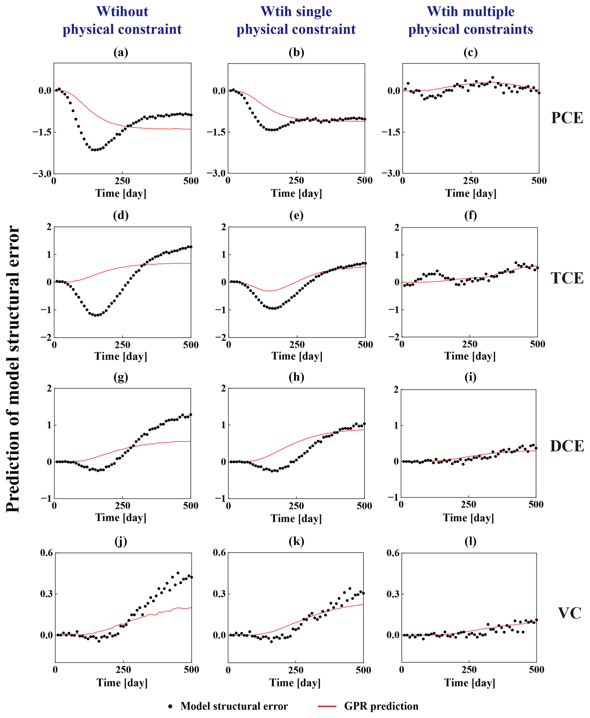
Figure 12 Predictions of model structural errors for the synthetic groundwater PCE reactive transport model without physical constraints (a, d, g, j), with single physical constraint (b, e, h, k) and with multiple physical constraints (c, f, i, l).

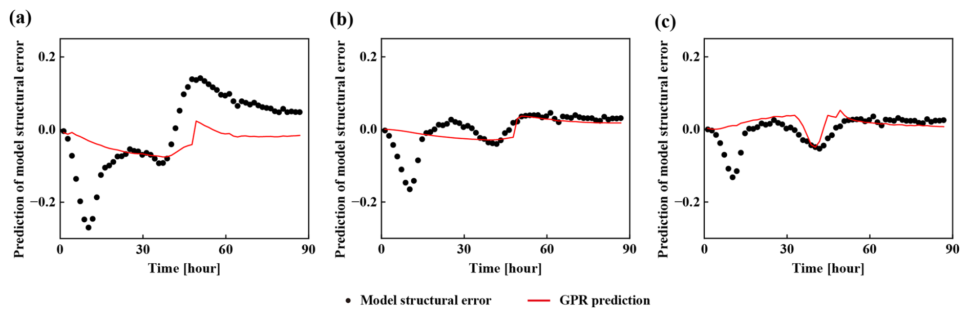
Figure 13 Predictions of model structural errors for the sand column Cd-phosphate cotransport model without physical constraints (a), with single physical constraint (b) and with multiple physical constraints (c).

5.4.3 Limitations of this Study

This study explicitly incorporates multiple physical constraints into the structural error correction process through a combined likelihood function, together with a dynamic sub-likelihood weight-updating strategy and associated stopping criterion, thereby overcoming the limitations of existing approaches in coupling multiple constraints. Unlike PIML approaches, the proposed method preserves the physical model predictions, with the corrected predictions consisting of the physical model, structural error, and measurement error, enhancing the robustness of extrapolative predictions. The proposed method primarily focuses on structural error correction and can adaptively correct structural error based on the discrepancy between physical model predictions and observations, providing a reasonable mechanism for structural error compensation. Unlike PIML approaches, which typically require the calculation of partial differential equation (PDE) residuals or modification of machine learning model architectures for specific problems, the proposed method can flexibly incorporate multiple physical constraints within a Bayesian framework. Moreover, it avoids the limitation of applying PIML to structural error correction, where physical constraints are imposed only on the error correction model rather than on the entire corrected prediction. Overall, this study provides a generalizable framework for enhancing predictive performance in simulations of contaminant reaction and transport within complex groundwater systems.

When the proposed method is applied to structural error correction in multicomponent reactive transport systems, multiple physical constraints typically need to be coupled simultaneously. In this context, the development of appropriate and effective physical constraints is essential. In general, the introduced constraints should exhibit clear mechanistic relevance to model structural error and observational data, and directly represent key physical processes that have been neglected or simplified. For instance, in more complex non-isothermal or multiphase flow systems, additional constraints may be needed to explicitly represent temperature-dependent transport and reaction processes, or the mass exchange and conservation of components across different phases. The constraints should also possess explicit physical meaning and quantifiable formulations to avoid imposing inappropriate restrictions. In addition, the effectiveness of physical constraints depends on the information they provide rather than simply on their number. When multiple physical constraints are introduced, emphasis should not be placed solely on increasing their number. Instead, the complementarity and potential competition among different physical constraints should be carefully evaluated to prevent redundant or conflicting constraints from adversely affecting parameter identification, thereby ensuring the physical consistency of the predictions.

Notably, although the effectiveness and generalizability of the proposed method have been demonstrated through two case studies, some limitations remain when applying the method to real contaminated sites and watershed-scale applications. Effective application of the method requires sufficient and representative observational data, reliable identification of the sources of model structural error, and strong relationships between the introduced physical constraints and structural error. In addition, an increase in the number of constraints inevitably increases the complexity of the combined likelihood function, resulting in higher computational cost and potentially affecting MCMC convergence. Future research may therefore explore approaches to internally quantify and correct structural errors within groundwater models, thereby reducing reliance on externally imposed physical constraints and improving the applicability and stability of structural error correction.

6 Conclusions

Using DDM to correct model structural errors provides an effective approach for improving the predictive performance of groundwater contaminant transport models. This study proposes a structural error correction framework capable of coupling multiple physical constraints, which has been demonstrated through two case studies. By constructing a combined likelihood function and dynamically updating sub-likelihood weights, the method explicitly incorporates multiple physical constraints into the structural error correction process, thereby substantially enhancing predictive accuracy and physical consistency of corrected predictions. The framework is demonstrated through two case studies: a synthetic three-dimensional PCE reactive transport simulation and a cadmium-phosphate cotransport sand column experiment. The main conclusions are summarized as follows:

1. An innovative data-driven framework is developed that couples multiple physical constraints through a combined likelihood function and dynamic updating of sub-likelihood weights. The structural error correction method exhibits broad applicability to complex multicomponent reactive transport systems.

2. The proposed dynamic weight-updating strategy with a stopping criterion maintains a balance between multiple physical constraints and observational information, thereby improving the robustness of parameter identification and constraint enforcement. Consequently, it enables the simultaneous coupling of distinct physical mechanism constraints.

3. The DDM coupled with multiple physical constraints effectively regulates parameter identification during structural error correction and suppresses excessive parameter adjustment. Consequently, the forms of structural errors in calibrated groundwater models become less complex and easier to characterize, leading to improved predictive accuracy and enhanced physical consistency of the corrected predictions.

4. Within the DDM framework for structural error correction, introducing appropriate physical constraints functions analogously to incorporating additional observations, thereby further reducing predictive uncertainty.