Towards a semi-asynchronous method for hydrological modeling in climate change studies

Hydrological impact assessments under climate change commonly rely on conventional modeling chains where climate projections are bias-corrected before being used in hydrological simulations. While this improves agreement with historical observations, it can introduce methodological uncertainties, reduce the diversity of climate ensembles, and smooth out extreme events. Asynchronous methods have been proposed as an alternative, allowing hydrological models to be calibrated directly with raw climate model outputs. However, fully asynchronous methods often fail to capture the timing of key hydrological processes, especially in snow-affected regions.

This study introduces and evaluates a semi-asynchronous calibration on monthly observed discharge distributions to address these limitations. Using the physically based WaSiM model, we compare the semi-asynchronous, fully asynchronous, and conventional methods across ten snow-influenced catchments in southern Quebec, Canada, under historical and future climate conditions.

The results show that while the fully asynchronous and semi-asynchronous methods perform well in preserving streamflow distributions and high-flow extremes, only the semi-asynchronous method succeeds in restoring the seasonal timing of key processes such as snowmelt and low flows. The semi-asynchronous method notably reduces intermodel variability in streamflow and snow water equivalent compared to the fully asynchronous approach. It also exhibits seasonal dynamics that closely align with observations and the conventional method, despite relying on uncorrected climate inputs. In contrast, the fully asynchronous method shows signs of desynchronization, with unrealistic snowmelt timing and elevated variability across projections. The conventional method, while more stable in the historical period, exhibits an increase in intermodel variability under future conditions, likely due to divergent magnitudes of projected change across climate models.

Compared to the conventional method, which benefits from stable and consistent simulations but tends to dampen extremes through bias correction, the semi-asynchronous approach offers a compelling alternative. It strikes a different balance between realism, ensemble diversity, and the ability to represent extreme flood events, making it particularly valuable for future-oriented climate impact assessments.

This study highlights the potential of the semi-asynchronous method as an innovative and robust tool for hydrological modeling under climate change. As climate model simulations continue to improve and their biases are progressively reduced, the semi-asynchronous approach is poised to benefit significantly, enhancing its potential for future hydrological projections.

1 Introduction

Climate change is one of the most significant challenges of our time, with profound implications for the Earth's hydrological systems. Alterations in temperature and precipitation regimes affect water availability and the timing of hydrological events. Understanding these impacts is crucial for effective water resource management and decision-making (Arsenault et al., 2013; Calvin et al., 2023). Accurate climate change studies are essential for developing strategies to mitigate and adapt to these changes, ensuring the sustainability of natural resources and the resilience of human and ecological systems (Milly et al., 2005; Sivakumar, 2011).

The complex dynamics of watersheds require hydrological models capable of precisely simulating both surface and subsurface processes (Farjad et al., 2016; Chu and Shirmohammadi, 2004). Accurate depiction of these processes within hydrological models is essential for assessing the impacts of climate change (Kour et al., 2016). Physically based and spatially distributed hydrological models, such as the Water Balance Simulation Model (WaSiM) (Schulla, 2021), are particularly valuable due to their detailed representation of key processes including surface runoff, groundwater recharge, interflow, and baseflow. These models further enable accurate simulation of hydroclimatic variables, which are essential for understanding the physical processes driving water flow and distribution within a catchment (Bormann and Elfert, 2010; Förster et al., 2017, 2018; Jasper et al., 2006; Natkhin et al., 2012). The use of physically based models like WaSiM, which capture local heterogeneity and finer-scale processes, provides a robust framework for evaluating climate change impacts on hydrology (Devia et al., 2015; Ludwig et al., 2009; Poulin et al., 2011) and supports stakeholders in making decisions that are both data-driven and aligned with strategic goals.

The conventional method for evaluating climate change impacts on hydrology involves a multi-step modeling chain designed to mitigate biases in both the hydrological model and the climate data. The method typically starts with the calibration of a hydrological model using observed meteorological data. Subsequently, raw climate model outputs are corrected using techniques such as quantile mapping (Themeßl et al., 2011; Mpelasoka and Chiew, 2009) to reduce potential biases with respect to the observed meteorological data. The calibrated hydrological model is then driven by these bias-corrected climate data to simulate hydrological processes over both a reference and a future period. By comparing the differences between these two periods, the method estimates the potential effects of climate change on hydroclimatic variables, enabling a clearer understanding of how projected climate change will influence key hydrological processes.

While widely used, conventional methods are constrained by both technical and subjective considerations, including modeling assumptions and methodological choices that can introduce uncertainty in the modeling chain (Moges et al., 2021). Bias correction can disrupt the physical consistency between simulated climate variables and affect long-term climate change signals (Chen et al., 2021; Lee et al., 2019). Advanced techniques, such as multivariate quantile mapping bias correction (MBCn) (Cannon, 2018), have been developed to address some of these issues while preserving inter-variable relationships, which are essential for reliable hydrological modeling. Additionally, the choice of bias correction method itself contributes to overall uncertainty in hydrological projections, as studies have shown that different correction techniques can alter streamflow estimates and influence the magnitude of projected hydrological impacts (Senatore et al., 2022). Also, conventional methods rely on high-quality meteorological observations, which are often unavailable in many regions (Ricard et al., 2023).

Asynchronous methods have been proposed to address some of these challenges (Ricard et al., 2019, 2020, 2023; Valencia Giraldo et al., 2023). This framework avoids the need for bias correction by adapting the hydrological model calibration process to directly use raw climate model projection data. This allows conducting climate change studies without relying on observed meteorological data or the underlying assumptions of conventional methods, albeit at the cost oftemporal synchronicity. Because the sequence of climatic events within climate model simulations is different from the historical observations, it is not possible to use the correlation between observed and simulated daily streamflow during the calibration process. Instead, the fully asynchronous method focuses on calibrating the statistical distribution of observed streamflow rather than reproducing historical time series. Given that most climate change impact studies assess the projected change in statistical properties between a reference and a future period (Piani et al., 2010), the need for accurate daily temporal correlation may become less critical (Ricard et al., 2019).

While fully asynchronous methods offer a promising alternative to conventional modeling chains by preserving the raw climate signal and streamflow distribution, they may do so at the expense of temporal coherence in hydrological processes, which can lead to inconsistencies in the timing of key processes such as snow accumulation and melt and subsequently affect other processes including streamflow, evapotranspiration and groundwater recharge. This study introduces a semi-asynchronous method that seeks to overcome this possible limitation by incorporating a calibration on monthly observed discharge distributions, thereby restoring seasonal alignment without relying on bias correction. Using the physically based WaSiM model, the study evaluates and compares the conventional, fully asynchronous, and semi-asynchronous methods across ten snow-influenced catchments in southern Quebec. The objective is to assess how each approach represents key hydroclimatic variables and seasonal processes under both historical and future climate conditions. The semi-asynchronous method emerges as a compelling compromise, retaining the advantages of the fully asynchronous framework while significantly improving temporal realism and reducing intermodel variability. This comparison provides valuable insights into the trade-offs between methodological simplicity, process fidelity, and ensemble diversity in hydrological climate change impact assessments.

2 Methods and data

2.1 Study area

The study focuses on a selection of forested catchments in Southern Quebec, Canada, chosen for their varied sizes and hydrological characteristics. These catchments range in area from 549 to 1910 km² (Table 1), providing a diverse representation of the region's physiographic and climatic conditions (Fig. 1). This subset was selected from catchments previously studied (Talbot et al., 2025b), where we have extensive knowledge of their behavior and a well-established baseline for comparison. These catchments are well-suited for hydrological modeling with WaSiM, as their natural hydrological processes remain largely intact and are minimally influenced by human-made structures such as dams. The availability of comprehensive streamflow data further supports their suitability for this study.

The Köppen-Geiger Climate Classification designates most of this region as Dfb (Humid Continental Mild Summer Wet All Year), with a smaller northern part classified as Dfc (Subarctic with Cool Summers and Year-round Precipitation) (Beck et al., 2018). Specifically, the Godbout, Matane, and Bonaventure catchments belong to the Dfc climate class, while all other catchments fall under the Dfb classification.

Climatic conditions show marked seasonal variations. Winters, extending from December to February, are cold with significant snowfall, contributing to the snowpack that influences spring runoff. Average temperatures during these months frequently drop below freezing, and snow depths can accumulate substantially, impacting streamflow upon melting.

Summers, from June to August, are characterized by warm temperatures and increased rainfall (Fig. 6). The transitional seasons of spring (March to May) and autumn (September to November) exhibit moderate temperatures and variable precipitation, playing a significant role in the hydrological cycle by contributing to groundwater recharge and streamflow variability.

Table 1 Physical and meteorological characteristics of the selected catchments in Southern Quebec.

^* Values are derived from WaSiM simulations (1981–2020) using ERA5 data downscaled to 1000 m × 1000 m. Values represent the average across all catchment pixels.

Figure 1 Locations of the selected catchments within Southern Quebec, Canada, outlined in red. The inset map provides the location of the study area within North America. The base map in this figure was created using ArcGIS^® software. Powered by Esri (https://www.esri.com, last access: 25 September 2024).

2.2 Data

2.2.1 Hydrometeorological data

This study utilizes daily total precipitation and mean temperature data from the ECMWF Reanalysis v5 (ERA5) (Hersbach et al., 2020) for the period 1981 to 2020. ERA5 was chosen due to its advanced features over previous reanalysis datasets, such as finer spatial resolution, hourly time step, and a more sophisticated data assimilation system that incorporates a wider range of observational inputs. These features make ERA5 a suitable reference dataset for hydrological modeling, as demonstrated in Tarek et al. (2020), where ERA5-based hydrological simulations performed equivalently to observational data in most regions, including our study area. Additionally, ERA5 showed reduced biases in temperature and precipitation compared to the ERA-Interim dataset, further justifying its use as a reliable and accurate source of climate data for climate change studies. While ERA5-Land offers finer resolution, ERA5 was deemed sufficient for this study since the region is not mountainous, and the focus is on long-term trends rather than specific events. The coarser resolution of ERA5 (31 km) still provides multiple grid points per catchment, allowing interpolation to match the model's resolution, making it an appropriate choice for our analysis.

Streamflow data was sourced from the Hydroclimatic Atlas of Southern Québec (MDDELCC, 2022), covering the period from 1981 to 2010. For each catchment, one hydrometric station located at the outlet was selected. This dataset provides daily measurements, though some catchments have minor gaps, primarily during winter months due to ice cover and ice jams. These periods were excluded from model calibration and analyses to maintain data accuracy.

2.2.2 Elevation

A hydrologically conditioned digital surface model (DEM) was derived from the NASA Shuttle Radar Topography Mission version 3.0 Global 1 arcsec (SRTMGL1). Hydrological corrections ensured accurate representation of hydrological networks, with adjustments made using SAGA GIS software (Conrad et al., 2015). Basin delineation and analysis were conducted using QGIS and Tanalys software (Schulla, 2021) to extract essential topographic information for hydrological modeling.

2.2.3 Soil type

Soil data were sourced from the SIIGSOL 100 m resolution database, which provides detailed descriptions of sand, clay, and silt proportions within the soil profile (Ministère des Ressources Naturelles et des Forêts, 2022; Sylvain et al., 2021). These proportions were converted to soil texture classes based on the USDA classification system. Soil hydraulic properties were imputed from established relationships between soil texture classes and hydraulic parameters (Weil and Brady, 2008). Elevation data were used to account for soil depth variability, by classifying raster cells into deep, normal, and shallow categories based on their relative elevation.

2.2.4 Land use

Land use data were obtained from the 2015 North American Land Change Monitoring System (NALCMS) 30 m resolution dataset. These data were resampled using the nearest neighbor method to create land use maps, significantly impacting hydrological parameters such as root distribution, vegetation cover fraction (VCF), roughness length (Z₀), and albedo. These parameters influence processes like evapotranspiration, runoff, and infiltration (Commission for Environmental Cooperation, 2015; Latifovic et al., 2012).

2.2.5 Climate model data

Projected daily temperature and precipitation data were sourced from the Coupled Model Intercomparison Project Phase 6 (CMIP6) (O'Neill et al., 2016) for both the reference period (1981–2010) and future period (2070–2099). These datasets were accessed and processed through the PAVICS-Hydro platform (Arsenault et al., 2023). The Shared Socioeconomic Pathway 5-8.5 (SSP5-8.5) scenario, which projects very high greenhouse gas emissions, was used to simulate future conditions (Calvin et al., 2023). To address uncertainties related to climate model selection, an ensemble of 18 climate models was employed as it was previously shown that, to ensure robustness, using multiple climate models is required (Arsenault et al., 2020; Lucas-Picher et al., 2021; Minville et al., 2008; Tarek et al., 2021). This ensemble approach ensures a more robust representation of potential climate outcomes by capturing a range of possible future scenarios. Table A1 provides a list of GCMs along with their respective institutions and horizontal resolutions.

To assess the reliability of the selected climate models, their ability to reproduce historical precipitation and temperature patterns was evaluated over the reference period (1981–2010). Tables A2 and A3 respectively present the monthly precipitation bias (%) and temperature bias (°C) for each model compared to ERA5, averaged across the 10 study catchments. These tables highlight seasonal discrepancies and allow the assessment of GCM performance. There is notable variability in precipitation biases among models. Some models, such as FGOALS-g3 and NorESM2-LM, exhibit consistently negative biases across most months (mean of bias of −16.4 % for both models). In contrast, IPSL-CM6A-LR and INM-CM4-8 show persistent overestimations, with mean biases of +17.5 % and +9.9 %, respectively. Temperature biases also show systematic trends, with models like EC-Earth3-Veg-LR and EC-Earth3 exhibiting cold biases below −2 °C, while MIROC6 and ACCESS-ESM1-5 systematically overestimate temperatures (mean of +1.8 % and +1.6 % respectively), particularly in summer. All models were retained to remain consistent with broader climate impact assessments and to ensure that the ensemble represents a wide range of potential climate outcomes. By including climate models with larger biases, we were also able to evaluate how each calibration method responds to diverse climate inputs and to test the robustness of the approaches under varying conditions. Climate model selection was not performed because the objective was not to develop a credibility-based climate change assessment, but rather to compare the behaviour of the three methods under a common ensemble spanning a wide range of biases. In practical applications, however, screening climate models based on their ability to reproduce key historical climatic features, such as seasonality, may help improve the reliability of hydrological simulations. More generally, when studies are intended to support climate change adaptation, selecting a more credible ensemble after historical evaluation of model performance may be preferable to using all models indiscriminately (Krysanova et al., 2018).

The resolution of the selected CMIP6 global climate models (GCMs) varies, with some models, such as IPSL-CM6A-LR, providing a finer resolution of 1.25° × 2.5°, while others, like CanESM5, retain a coarser resolution of 2.8° × 2.8°. Given that the hydrological model operates at a 1000 m spatial resolution, a method was required to bridge the resolution gap between GCMs and WaSiM. To address this, WaSiM internally applies inverse distance weighting (IDW) interpolation, ensuring that the coarse-resolution GCM data is adjusted to match the finer hydrological grid. This approach ensures that all methods remain comparable by using climate models at the same spatial resolution. External statistical or dynamical downscaling methods were deliberately avoided to maintain methodological consistency between the three methods. Additionally, since this study focuses on 30-year climatological trends rather than individual events, the impact of finer-resolution climate inputs is expected to be minimal when averaged over long periods.

2.3 Hydrological modeling

2.3.1 Hydrological model

WaSiM is a physically based, spatially distributed hydrological model designed to simulate water flow processes in catchments. It integrates a comprehensive suite of sub-models to capture key hydrological processes, including surface runoff, groundwater recharge, interflow, and baseflow, within a deterministic framework (Schulla, 2021). In this study, WaSiM was configured with a spatial resolution of 1000 m and a temporal resolution of 24 h. This setup allows for detailed spatial analysis while maintaining computational efficiency. The chosen spatial resolution ensures that the heterogeneity of the landscape is adequately captured, and the daily time step allows for accurate simulation of hydrological processes over time. WaSiM employs the Richards equation and the Van Genuchten parameters for simulating water flow in the unsaturated zone (van Genuchten, 1980; Richards, 1931). This equation provides a physically based representation of hydraulic head gradients and soil moisture dynamics, incorporating detailed soil physical properties. Groundwater flow is calculated conceptually within the unsaturated zone model.

2.3.2 Conventional method

The framework used to calibrate and validate the effectiveness of the conventional method rely on the split sample test (SST) approach, which is widely recognized for its effectiveness in evaluating model performance. This approach involves dividing the data into separate calibration and validation periods, allowing for an assessment of the model's ability to generalize beyond the calibration conditions. For this method, historical data from ERA5 were used for both calibration and validation. The calibration period spanned from 2000 to 2009, during which simulations were performed over a 15-year period (1995 to 2009), discarding the first 5 years to stabilize the initial conditions of the model. The validation period was set from 1990 to 1999, following the same approach of conducting simulations over a 15-year period (1985 to 1999) and discarding the initial 5 years.

A set of 17 parameters (Table 2) was selected for calibration based on model documentation. Table 2 was taken from Talbot et al. (2025a).

Table 2 Calibration parameters for the hydrological model WaSiM.

^* Calibration coefficient, ranging from 0.8 to 1.4, is applied to adjust the total soil depth, which is predetermined to be 8 m for shallow, 14 m for normal, and 20 m for deep soil conditions.

These parameters were optimized based on a single objective function through the Dynamically Dimensioned Search (DDS) algorithm, developed by Tolson and Shoemaker (2007). This algorithm was chosen for its efficiency in handling complex optimization problems for compute-intensive hydrological models, as recommended by Arsenault et al. (2014).

The objective function used for calibration was the Kling Gupta-Efficiency (KGE) (Kling et al., 2012). The KGE metric provides a balanced evaluation of model performance by considering simultaneously correlation, variability, and bias in the simulated streamflow relative to observed streamflow. The KGE is computed using Eq. (1):

$$\begin{array}{}\text{(1)}& \mathrm{KGE}=\mathrm{1}-\sqrt{{\left(r-\mathrm{1}\right)}^{\mathrm{2}}+{\left({\displaystyle \frac{{\mathit{\sigma }}_{\mathrm{sim}}/{\mathit{\mu }}_{\mathrm{sim}}}{{\mathit{\sigma }}_{\mathrm{obs}}/{\mathit{\mu }}_{\mathrm{obs}}}}-\mathrm{1}\right)}^{\mathrm{2}}+{\left({\displaystyle \frac{{\mathit{\mu }}_{\mathrm{sim}}}{{\mathit{\mu }}_{\mathrm{obs}}}}-\mathrm{1}\right)}^{\mathrm{2}}},\end{array}$$

where r is the Pearson correlation coefficient between simulated and observed streamflow, σ_sim is the standard deviation of simulated streamflow, σ_obs is the standard deviation of observed streamflow, μ_sim is the mean of the simulated streamflow, and μ_obs is the mean of the observed streamflow. A KGE value of 1 indicates a perfect match between the simulated and observed streamflow, reflecting ideal performance across all three components: correlation, variance, and bias.

For the conventional method, the Multivariate Bias Correction algorithm (MBCn) developed by Cannon (2018) was used to correct biases in the climate model simulations. This method corrects biases in meteorological data while accounting for spatiotemporal interdependencies between variables and preserving changes in quantiles between the reference (1981–2010) and future (2070–2099) periods. The bias correction was applied to daily total precipitation and daily mean temperature using ERA5 data as the reference over the period 1981–2010 and was used to correct the climate models data for both the reference (1981–2010) and future periods (2070–2099). Climate change impact assessments were subsequently conducted using bias-corrected climate model data. Hydrological simulations were performed for each climate model over both the reference and future periods, using a hydrological model calibrated with observed meteorological data for each catchment.

2.3.3 Fully asynchronous method

The primary objective of the fully asynchronous method is to conduct climate change studies without relying on observed meteorological data (Ricard et al., 2019, 2020, 2023; Valencia Giraldo et al., 2023) and eliminate the need for bias-correction of climate variables. Instead, the calibration is performed using raw climate model data and observed streamflow, integrating the bias-correction in the calibration step. A significant challenge in this approach is the lack of synchronization between the timings of observed streamflows and those of raw climate model outputs (Ricard et al., 2019), as climate models are not temporally aligned with actual past events. This requires a departure from the conventional calibration framework, which aims to optimize the timing and amplitude of streamflow. To overcome this obstacle, the objective function optimizes the distribution of observed streamflow over an extended period rather than individual streamflow observations. This approach ensures that the hydrological model effectively preserves the streamflow distribution, rather than capturing day-to-day natural variability. Figure 2 presents a workflow diagram of the fully asynchronous method, adapted from Ricard et al. (2023).

Figure 2 Workflow diagram of the fully asynchronous method.

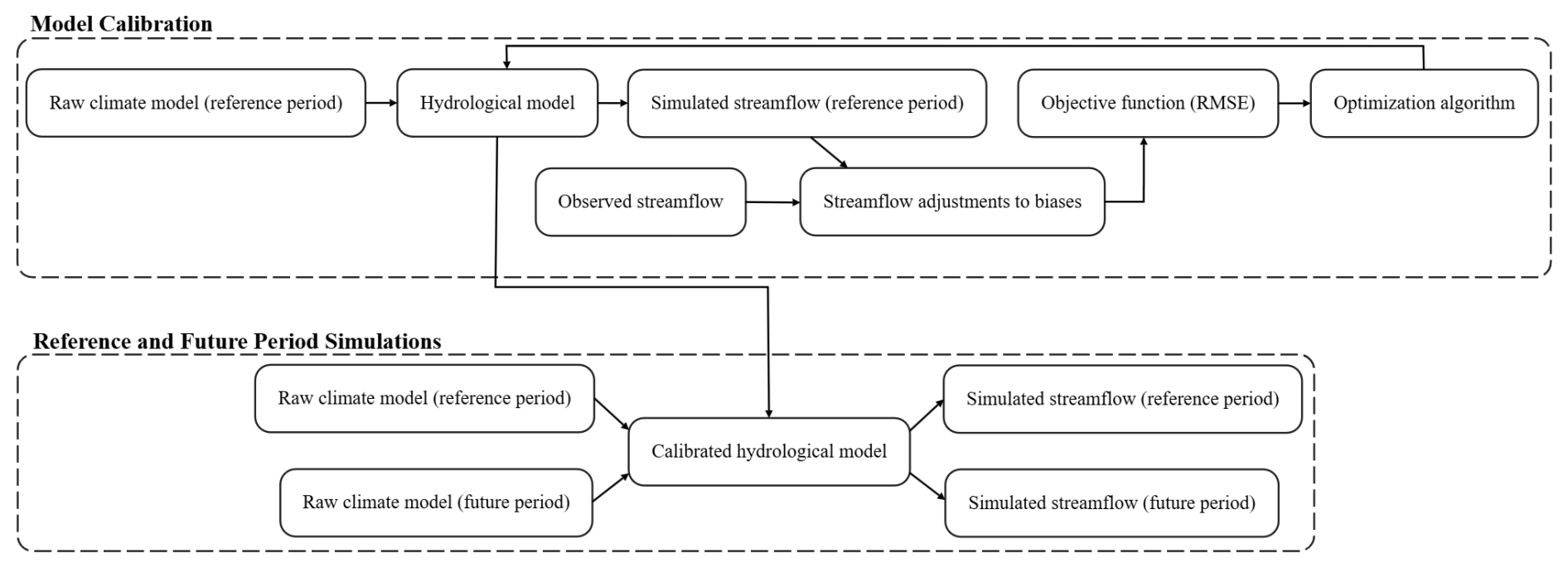
Given the calibration objectives of the fully asynchronous method, the observed streamflow data for a 26-year period (1984–2009) was sorted and used to establish a reference distribution of streamflow. This sorted distribution provided a consistent target for both the calibration and validation of the hydrological model. In the context of the fully asynchronous method, where direct temporal alignment between climate model outputs and observed streamflow is not maintained, relying on the same observed distribution for both calibration and validation ensures that the model is evaluated against a stable and representative reference. Therefore, the 26-year period of hydrometric station data was selected for calibration and validation to capture a wide range of hydrological conditions. This duration helps reduce the impact of short-term climate variability and minimizes biases associated with shorter time frames. A key hypothesis underlying this approach is the assumption of stationarity, that the hydrological model, with fixed parameters optimized during calibration, will continue to produce reasonable streamflow simulations under future climate conditions. This assumes that despite changing climatic conditions, the model will adequately respond to future scenarios as it did to past conditions. However, if future climate changes introduce conditions outside the model's calibrated range, such as new snow patterns or shifts in seasonal dynamics, the model's performance could be compromised. It is important to recall that the conventional method also relies on two stationarity assumptions, namely that the calibrated parameters of the hydrological model remain valid under future conditions and that the bias correction applied to the climate data continues to hold under a changing climate.

The calibration and validation periods are separated based on the total yearly precipitation from October to September. This separation ensures an equal distribution of wet and dry years between both periods. More specifically, yearly precipitation totals were first ranked from the driest to the wettest years, and one year out of every two in this ordered series was selected for calibration. This procedure resulted in 13 non-consecutive calibration years distributed across the full range of hydroclimatic conditions. Simulations were performed for the years 1984 to 2011, using raw climate model outputs, with the first two years discarded to allow for initial model stabilization. Out of the 26 years of simulations, 13 years were used for calibration, selected based on total yearly precipitation, while the remaining 13 years were used for validation.

To address biases in simulated streamflow resulting from biases in raw climate data, the simulated streamflow was adjusted by multiplying it by a factor equal to the ratio of the mean observed streamflow Q_obs to the mean simulated streamflow Q_sim. This adjustment was applied only during the calibration and validation process and not during the reference or future periods simulations. It ensures that the mean simulated streamflow matches the mean observed streamflow, effectively removing bias and allowing the optimization algorithm to focus on matching the shape of the streamflow distribution rather than its absolute magnitude. This means the simulated absolute streamflow values cannot be directly compared with observations, but changes between the reference and future period can be analyzed.

An essential aspect of the fully asynchronous method is its focus on calibrating the model based on the distribution of streamflow rather than its temporal sequence. Given this objective, Root Mean Square Error (RMSE) was selected as the calibration metric due to its ability to emphasize overall distributional accuracy while penalizing large deviations between simulated and observed streamflow values. RMSE effectively captures the spread and magnitude of streamflow across different flow conditions, ensuring that extreme and median flows are well represented. Unlike correlation-based metrics, which prioritize timing accuracy, RMSE remains robust when applied to sorted streamflow values, aligning well with the fully asynchronous method's goal of preserving statistical consistency rather than event-specific timing. Additionally, RMSE provides a straightforward optimization framework, allowing for efficient parameter tuning without introducing unnecessary complexity into the calibration process. The RMSE was computed on the flow duration curves of the simulated and observed flows using Eq. (2):

$$\begin{array}{}\text{(2)}& \mathrm{RMSE}=\sqrt{{\displaystyle \frac{\mathrm{1}}{n}}{\sum }_{i=\mathrm{1}}^n{\left({\left(\mathrm{sort}(Q_{\mathrm{sim}}\right)}_i-{\left(\mathrm{sort}(Q_{\mathrm{obs}}\right)}_i\right)}^{\mathrm{2}}},\end{array}$$

where Q_sim represents the simulated streamflow (mm), Q_obs represents the observed streamflow (mm), sort() is the function that sorts the sequence in descending order, and n is the number of simulated streamflow values.

Each climate model was calibrated for each catchment, resulting in a total of 180 calibration parameter sets (18 climate models × 10 catchments). In contrast, the conventional method involves 10 calibration parameter sets (one per catchment) which is then applied to all climate models and their bias-corrected outputs. Consequently, the fully asynchronous method is considerably more computationally intensive than the conventional method in terms of parameter calibration.

The calibration framework for the fully asynchronous method is similar to that of the conventional method (Sect. 2.3.2). It involves 1000 evaluations, uses the same 17 calibration parameters (Table 2), and employs the DDS optimization algorithm.

For the fully asynchronous method, climate change simulations were conducted using the calibrated model for each catchment and each projected climate model, but without relying on historical event timing. Raw projected climate data were utilized to perform simulations over both the reference and future periods.

2.3.4 Semi-asynchronous method

In addition to the conventional and fully asynchronous approaches, a semi-asynchronous method was developed and tested in this study. This method follows the same overall framework as the fully asynchronous approach but introduces an element to account for temporal dependencies in the objective function used during calibration. Specifically, rather than computing the RMSE over the entire streamflow distribution, the RMSE is calculated on the sorted streamflow separately for each calendar month, thereby capturing seasonal variations more explicitly. The overall objective function for the semi-asynchronous method is defined as a weighted average of monthly RMSE values, as shown in Eq. (3):

$$\begin{array}{}\text{(3)}& {\mathrm{RMSE}}_{\mathrm{sa}}={\displaystyle \frac{\mathrm{1}}{\mathrm{12}}}{\sum }_{m=\mathrm{1}}^{\mathrm{12}}({\mathit{\alpha }}_m\times {\mathrm{RMSE}}_m)\end{array}$$

In this equation, RMSE_sa is the semi-asynchronous RMSE used as the objective function, and RMSE_m refers to the RMSE between the sorted simulated and observed streamflow values for calendar month m, from January to December, as detailed in Eq. (2). α_m is equal to 1 and represents a weighting coefficient that determines the importance of that month in the overall calibration. By grouping streamflow values by month and comparing the corresponding sorted distributions, the semi-asynchronous method introduces partial synchronicity into the calibration process. The proposed design preserves the underlying hypothesis of the fully asynchronous method in reproducing streamflow distributions, while also incorporating seasonal characteristics of key hydrological events. The monthly discretization was selected to capture key seasonal hydrological processes while maintaining enough data points within each subset for robust distribution estimation. Although other temporal aggregations could be considered, such as sub-monthly periods, or moving windows, for example a 30-day window with daily or weekly shifts, they are not expected to alter the main conclusions of this study.

2.4 Comparative analysis

The analysis in this study is designed to compare the performance of the conventional, fully asynchronous, and semi-asynchronous methods in simulating hydrological processes under both current and future climate conditions. To ensure a fair and unbiased comparison, all three methods employed the same WaSiM configuration, including identical calibration parameters, the number of evaluations, and the optimization algorithm. This was performed to ensure minimal calibration bias and to isolate the differences attributable solely to the methodological framework of each approach.

The first step in the analysis involves assessing the calibration and validation performance of each method. Streamflow simulations were evaluated using the Kling-Gupta Efficiency (KGE) for the conventional method and the root mean square error (RMSE) between sorted simulated and observed streamflow values for both the fully asynchronous and semi-asynchronous methods. These metrics were selected to highlight each method's respective strengths, with KGE capturing overall model performance and RMSE emphasizing accuracy in reproducing the streamflow distribution.

Beyond streamflow, the relationships between various hydroclimatic variables, such as groundwater recharge, surface runoff, soil moisture, and snow water equivalent (SWE) were also examined. By comparing the simulated values from all three methods, the analysis seeks to understand how well each method captures the interactions between these variables. This serves to evaluate the internal consistency of the models and assess their ability to realistically simulate the physical processes within the catchments.

The analysis extends to a comparison of the projected changes in hydroclimatic variables between the reference period (1981–2010) and the future period (2070–2099). The magnitude and direction of these changes are assessed to determine how each method projects the impact of climate change on the catchment's hydrological processes. This includes examining variables such as changes in snowmelt dynamics and the consequent effects on streamflow, surface runoff and groundwater recharge. A detailed spatial analysis is also conducted to evaluate the distribution of such key variables across the catchments. The comparative analysis employs several criteria to determine which method is most effective. These include the accuracy of streamflow simulation (both in terms of overall distribution and event timing), the internal consistency of hydroclimatic variable relationships and the realism of spatial distributions and projected changes under future climate scenarios.

3 Results

3.1 Streamflow representation

For the conventional method, streamflow representation performance was assessed using the KGE metric for each catchment during both the calibration and validation periods.

During calibration, the conventional method achieves KGE values ranging from 0.817 to 0.906, with a mean of 0.863. Similarly, for the validation period, the KGE values ranged from 0.778 to 0.906, with a mean of 0.842. These results indicate that the conventional method maintains a consistent performance in simulating streamflow across different catchments. Detailed KGE results for each catchment are provided in the Appendix B (Table B1).

For the fully asynchronous and semi-asynchronous methods, streamflow representation performance was evaluated using the RMSE calculated on sorted daily streamflow values. For the fully asynchronous method, the mean RMSE during calibration was 0.121 mm d⁻¹, with an inter-model standard deviation of 0.031 mm d⁻¹. In the validation period, the mean RMSE increased slightly to 0.287 mm d⁻¹, with a standard deviation of 0.095 mm d⁻¹. The semi-asynchronous method showed higher RMSE values overall, with a mean of 0.282 mm d⁻¹during calibration and 0.348 mm d⁻¹ during validation. To enable direct comparison, the sorted RMSE was also computed for the conventional method, yielding values of 0.497 mm d⁻¹ for calibration and 0.518 mm d⁻¹ for validation. These results indicate that, in terms of streamflow distribution alone, the fully-asynchronous method performed best, followed by the semi-asynchronous method, and finally the conventional method. This ranking highlights the strengths of the distribution-focused calibration used in the fully asynchronous approaches. However, this comparison should be interpreted with caution, as the better RMSE performance of the asynchronous methods is expected given that RMSE on streamflow distributions is directly aligned with their calibration objective, unlike for the conventional method. Detailed RMSE results for all methods and catchments are provided in Appendix B (Table B2).

Figure 3 presents hydrographs of streamflow for all three methods during the reference period across the ten catchments, along with observed streamflow for the same period. The fully asynchronous method shows greater variability between climate models, especially in the timing of peak flows, which often fails to align with the observed data, as expected. This variability suggests that the timing of streamflow events in the fully asynchronous method is highly sensitive to the specific climate model employed. For instance, in the Matane catchment, the observed and conventional method peak flow occurs at the beginning of May, while the fully asynchronous method shows a broader range of peak flow timings, extending from early May to late June. This discrepancy might be attributed to challenges in accurately simulating snowmelt processes with the fully asynchronous method, which are crucial for generating high flows in snowy catchment. Furthermore, in the same catchment, the fully asynchronous method overestimates summer flows compared to the observed data, indicating potential difficulties in capturing the seasonal dynamics of low-flow periods. Conversely, the semi-asynchronous and conventional methods both succeed in capturing the seasonal timing and magnitude of streamflow events, closely aligning with the observed hydrographs. The conventional method offers the most consistent performance across climate models, with peak flows and low-flow periods well synchronized with observations on the reference period. The semi-asynchronous method also accurately reproduces the overall seasonal streamflow pattern, including the timing of snowmelt-driven peak flows. Although it introduces slightly more inter-model variability than the conventional method, this variability remains lower than that observed in the fully-asynchronous method.

Figure 3 Seasonal streamflow comparison between the fully asynchronous, semi-asynchronous and conventional methods and observed data across ten catchments during the reference period (1981–2010). The panels (a)–(j) represent the catchments of Bonaventure, Matane, Ouelle, Bécancour, Nicolet SO, Au Saumon, Bras du Nord, Du Loup, Valin, and Godbout, respectively.

Figure 4 presents the relationship between sorted streamflow values and percentage bias for simulated versus observed streamflow using the three methods during the reference period (1981 to 2010) for the Matane catchment. The fully asynchronous method shows the lowest percentage bias across a wide range of streamflow conditions, particularly at the extremes, reflecting its strong ability to capture the full distribution of flows. This performance stems from its calibration strategy, which explicitly targets the statistical distribution of streamflow rather than the timing of individual events.

The semi-asynchronous method offers intermediate performance between the fully asynchronous and conventional methods. It more accurately represents the streamflow distribution than the conventional approach, particularly for high and low flows, but shows slightly greater bias than the fully asynchronous method. This outcome suggests that the incorporation of monthly structure into the calibration helps preserve distributional accuracy while also improving the temporal realism of seasonal flow patterns. In contrast, the conventional method shows broader dispersion in bias and tends to underperform in reproducing extreme events, especially at high flows. While Fig. 4 focuses on the Matane catchment, similar patterns are observed across the other study catchments (Figs. C1 to C9), reinforcing the generalizability of these results. Together, these findings highlight a key trade-off in hydrological modeling under climate change, where the fully asynchronous method excels in preserving streamflow distribution and extremes, the conventional method performs best in capturing temporal accuracy, and the semi-asynchronous method offers a promising compromise by balancing both aspects.

Figure 4 Performance comparison between the conventional, fully asynchronous and semi-asynchronous methods for the Matane catchment during the reference period (1981–2010). The figure shows the percentage bias between observed and simulated streamflows, with the x-axis representing the observed daily streamflow and the y-axis displaying the percentage bias relative to the observed values. The shaded regions illustrate the variability among climate models around the mean bias for each method (solid lines).

Figure 5 presents a comparative analysis of streamflow quantiles simulated by the three methods across the reference period (1981 to 2010) and the future period (2070 to 2099) for all ten catchments. When comparing the reference period simulations to observed streamflow, both the fully asynchronous and semi-asynchronous methods demonstrate closer alignment with the observed distribution, particularly for high flows (Q₉₅). This confirms their ability to better capture streamflow extremes. Specifically, the absolute median bias for Q₉₅ is 1.6 % for the fully asynchronous method and 2.8 % for the semi-asynchronous method, compared to 4.7 % for the conventional method (Table D1). However, this improved accuracy comes with greater inter-model variability. For Q₉₅ in the reference period, the standard deviation across climate models increases from 3.3 % with the conventional method to 4.8 % with the semi-asynchronous method and 4.0 % with the fully asynchronous method.

In terms of future projections, all methods show a decrease in Q₉₅ across most catchments. The fully asynchronous method estimates a smaller reduction in Q₉₅ at 8.6 %, while the semi-asynchronous and conventional methods project declines of 8.6 % and 14.1 %, respectively (Table D1). Despite the more moderate change, the semi-asynchronous method shows the highest inter-model variability, with a standard deviation of 19.1 %, while the fully asynchronous and conventional methods display similar and lower variability, at 10.5 % and 9.7 %, respectively.

For median flows (Q₅₀), the results are more varied. During the reference period, the semi-asynchronous method achieves the lowest absolute median bias at 2.3 %, followed by the fully asynchronous method at 4.1 %, and the conventional method at 12.1 % (Table D2). Under future conditions, all three methods project an increase in Q₅₀, with the semi-asynchronous method projecting the largest rise at 24.1 %, followed by the conventional method at 18.0 % and the fully asynchronous method at 16.8 %. The semi-asynchronous method also displays the highest inter-model spread, with a standard deviation of 31.2 %, compared to 16.6 % for the conventional method and 16.9 % for the fully asynchronous method.

Low flows (Q₅) reveal the largest discrepancies among methods. In the reference period, the fully asynchronous method shows the lowest absolute median bias at 33.0 %, followed by the conventional method at 57.3 %, and the semi-asynchronous method at 71.5 % (Table D3). These results highlight the difficulty of all methods to accurately capture low-flow conditions. These large low-flow biases likely reflect the fact that the objective functions used in this study place greater emphasis on medium and high flows, making all methods less sensitive to errors under low-flow conditions. For future projections, Q₅ decreases by 25.2 % for the conventional method, 2.3 % for semi-asynchronous and 9.9 % for the fully asynchronous method. Once again, the fully asynchronous and semi-asynchronous methods display higher variability, with standard deviations of 25.0 % and 24.3 % respectively, compared to 9.8 % for the conventional method.

Overall, the quantile-based analysis highlights the strength of the fully asynchronous and semi-asynchronous methods in capturing flow distributions and extremes, while also emphasizing their increased sensitivity to climate model variability. Detailed results across all ten catchments are provided in Tables D1 to D3.

Figure 5 Comparison of streamflow distributions for the reference period (1981–2010) and projected changes in the future period (2070–2099) across 10 catchments. The plots show the percentage differences in streamflow quantiles between simulated and observed values during the reference period, and the projected changes represent the percentage differences between future and reference simulations for each method. Boxes indicate the interquartile range (25th to 75th percentiles), and central lines represent the median. For a more detailed quantification, refer to Tables D1–D3.

3.2 Hydroclimatic variables

In addition to streamflow, a key objective of this study is to evaluate how well the conventional, fully asynchronous, and semi-asynchronous methods simulate a broader range of hydroclimatic variables. This allows for a more comprehensive comparison of the methods' ability to reproduce the underlying hydrological processes that govern catchment behavior under current and future climate conditions.

To explore these dynamics in greater detail, the Matane catchment was selected as a representative case study. Covering an area of 1650 km², Matane exhibited strong calibration and validation performance across all three methods and reflects the typical hydroclimatic and physiographic conditions found across the study region. This focused analysis enables a deeper examination of how each method influences key components of the water balance, including snowmelt, surface runoff, evapotranspiration, groundwater recharge, and soil moisture.

Average monthly temperature and precipitation for the reference period (1981–2010) and the future period (2070–2099) before and after bias-correction using MBCn for the Matane catchment and the climate model ACCESS-ESM1-5 is provided as an example (Fig. 6).

In the reference period, a noticeable gap exists between the ERA5 data and the raw climate model data, with the raw climate data showing higher temperatures and increased precipitation for all months except October. The effectiveness of the bias correction is evident, as the bias-corrected climate data closely aligns with the ERA5 data, significantly reducing discrepancies in temperature and precipitation. The same bias trend is observed in the future period, where raw climate model data predicts higher temperatures and increased precipitation compared to the bias-corrected data.

Furthermore, Fig. 6 highlights the anticipated changes in precipitation and temperature between the reference and future periods. Temperatures are expected to increase significantly, with projected increases around 6 °C across the study area. These projections are in line with the IPCC's forecasts based on SSP5-8.5, and suggest that northern latitudes will experience faster warming compared to the global average (Estrada et al., 2021). Projections consistently show an annual increase in precipitation ranging from 15 % to 20 %, with the most significant increases occurring between November and April, as well as in July. The anticipated increases in temperature and changes in precipitation patterns have profound implications for hydrological processes and water resource management.

Figure 6 Comparison of average monthly precipitation and temperature for the Matane catchment. Bars represent monthly total precipitation (mm), while lines represent monthly mean temperature (°C). Black corresponds to the ERA5 reference dataset. Green shades represent bias-corrected climate model simulations (reference and future periods), while red shades represent raw climate model outputs (i.e., without bias correction). Darker colors indicate the reference period (1981–2010), and lighter colors indicate the future period (2070–2099) under the SSP5-8.5 scenario.

Table 3 presents the annual averages of key hydroclimatic variables for both the reference period (1981 to 2010) and the future period (2070 to 2099). All three methods, project similar directional changes under future climate conditions. Precipitation and ETa are projected to increase, while snowfall and SWE decline significantly. These changes are consistent with the expected response to warming, where higher temperatures reduce snow accumulation and increase atmospheric demand for water. For instance, SWE decreases by more than 50 % across all methods, while ETa increases by approximately 31 %–32 %.

Despite these common trends, notable differences are observed in the magnitude and representation of certain variables. Surface runoff stands out as the most divergent. The fully asynchronous method simulates more than twice the amount of surface runoff compared to the conventional method during the reference period, a pattern that persists in future projections. This discrepancy could be due to the fully asynchronous method's misrepresentation of the timing of snowmelt, leading to amplified runoff responses. The semi-asynchronous method moderates this behavior, producing runoff values that are closer to those of the conventional method, although still elevated. This suggests that the inclusion of monthly calibration in the semi-asynchronous method helps correct some of the temporal misalignments present in the fully asynchronous approach.

Groundwater recharge also shows significant differences. The fully asynchronous method simulates a relatively large increase of 19 % between the reference and future periods, compared to only 4 % with the conventional method. The semi-asynchronous method again produces an intermediate value of 9 %. Similar patterns are observed in other components of the water balance.

Streamflow values appear relatively consistent across methods and periods, with projected changes ranging from 1 % to 2 %. Soil moisture shows smaller differences between methods, although the semi-asynchronous method again occupies an intermediate position.

Table 3 Comparison of hydroclimatic variables between the reference (1981–2010) and future (2070–2099) periods for the conventional, fully asynchronous and semi-asynchronous methods across 10 catchments and 18 climate models.

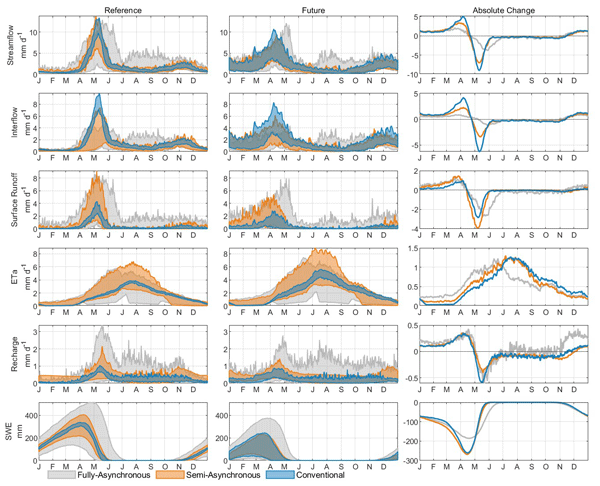
Figure 7 illustrates the annual cycle of key hydroclimatic variables in the Matane catchment for both the reference period (1981–2010) and the future period (2070–2099). Equivalent figures for the other catchments are available in Appendix E.

Focusing first on the reference period, the fully asynchronous method stands out for its high inter-model variability, particularly in snow dynamics. The timing of maximum SWE varies widely, with some models showing snowmelt beginning as early as late April and extending into July. This prolonged melt period is unrealistic for the Matane region, where snow typically disappears by the beginning of June. Such an extended melt season in a 30-year average suggests a clear limitation of the fully asynchronous method in accurately capturing seasonal snow processes.

This misrepresentation has cascading effects on other components of the hydrological cycle. Surface runoff, actual evapotranspiration, and groundwater recharge simulated by the fully asynchronous method also exhibit elevated variability and inconsistencies. In its effort to reproduce the observed streamflow distribution without aligning events temporally, the fully asynchronous method tends to distort internal processes, leading to simulations that lack physical plausibility and seasonal coherence. These shortcomings undermine confidence in the method's use for climate change impact assessments in snow-dominated regions.

In contrast, the semi-asynchronous method substantially reduces the inter-model variability observed in the fully asynchronous approach, particularly for streamflow and SWE. Snowmelt timing is notably improved, aligning more closely with expectations for the Matane catchment. This correction enhances the seasonal dynamics of streamflow and groundwater recharge, making the simulations more physically realistic. However, some issues remain. The semi-asynchronous method still shows greater variability in ETa compared to the conventional method. This is likely due to the use of raw, uncorrected climate model inputs in both asynchronous approaches, whereas the conventional method benefits from bias-corrected meteorological data. The model compensates for climate model biases by adjusting evapotranspiration to close the water balance, which can lead to unrealistic variability for this variable. The conventional method produces well-defined spring peaks in streamflow and interflow with lower inter-model variability. Its outputs are more consistent across models, enhancing confidence in its projections.

For the future period, the semi-asynchronous and conventional methods produce similar results for SWE, streamflow, and groundwater recharge, though the semi-asynchronous method shows greater variability in surface runoff and ETa. Compared to the reference period, the conventional method exhibits an increase in inter-model variability, which can be attributed to the fact that bias correction constrains variability under historical conditions but does not limit the divergence of climate model projections in the future. The fully asynchronous method continues to exhibit the highest variability across climate models, further diminishing confidence in its outputs.

Regarding the absolute changes between the reference and future periods, the semi-asynchronous and conventional methods yield comparable trends for SWE and groundwater recharge. The semi-asynchronous method produces slightly smaller variations in absolute change for streamflow and interflow, but slightly larger variations for surface runoff. Due to the high variability observed in both the reference and future periods, the fully asynchronous method offers limited reliability in its estimates of absolute change. Taken together, these results confirm that while the semi-asynchronous method offers clear improvements over the fully asynchronous approach, particularly in representing snowmelt and reducing variability, it does not yet match the stability or reliability of the conventional method for detailed climate impact assessments.

Figure 7 Seasonal distribution of key hydroclimatic variables for the reference period (1981–2010), future period (2070–2099), and their average absolute changes across the Matane catchment. The left column shows simulations during the reference period, the middle column corresponds to the future period, and the right column displays the absolute change between the two. Shaded areas represent the spread across the 18 climate models.

Figure 8 illustrates the spatial distribution of annual groundwater recharge rates in the Matane catchment for both the reference (1981–2010) and future (2070–2099) periods, based on simulations from the conventional, fully asynchronous, and semi-asynchronous methods. All methods exhibit similar spatial patterns, with higher elevations showing reduced recharge rates and lower elevations demonstrating higher recharge rates. An elevation map of the Matane catchment is provided in the Appendix F (Fig. F1). The semi-asynchronous method, however, predicts a generally higher magnitude of recharge across the catchment.

When examining the absolute difference between the future and reference periods, all methods project a similar spatial pattern of changes in groundwater recharge, with a noticeable decrease in recharge at lower elevations. However, the fully asynchronous and semi-asynchronous methods project smaller increases in recharge in certain higher elevation areas, while the conventional method predicts a much more pronounced reduction, 3 to 4 times greater, at lower elevations.

Figure 8 Spatial distribution of annual groundwater recharge in the Matane catchment for the reference period (1981–2010) and future period (2070–2099).

Figure 9 illustrates the spatial distribution of soil moisture across the Matane catchment for both the reference period (1981–2010) and the future period (2070–2099), comparing results from the conventional, fully asynchronous and semi-asynchronous methods. All three methods demonstrate that soil moisture distribution is heavily influenced by soil type, as indicated by the consistent spatial patterns observed (detailed soil type information is provided in the Appendix F, Fig. F1). The soil moisture maps show that areas with finer soils, such as loam, tend to have higher moisture retention, while coarser soils, such as sandy loams, exhibit lower moisture levels.

The fully asynchronous method tends to generate slightly higher soil moisture values compared to the other two methods, particularly in areas with inherently higher moisture retention capacity. The fully asynchronous method also displays greater variability in soil moisture patterns.

In terms of absolute changes between the reference and future periods, all three methods project a decrease in soil moisture between the reference and future periods, with generally consistent spatial patterns across methods. The magnitude of change differs, however, with the conventional method showing values closer to those of the fully asynchronous method, while the semi-asynchronous method exhibits smaller absolute changes overall. Additionally, the fully asynchronous method presents localized areas with slight increases in soil moisture, a feature that is less pronounced in the other two methods. Finally, it is noteworthy that the patterns of groundwater and soil moisture during the reference and future periods are spatially consistent and exhibit similar trends.

Figure 9 Spatial distribution of relative soil moisture in the Matane catchment for the reference period (1981–2010) and future period (2070–2099).

4 Discussion

The primary goal of this study was to evaluate the ability of the fully asynchronous and semi-asynchronous methods to reproduce key hydrological processes within catchments, in comparison to the conventional approach. By conducting detailed analyses across ten catchments and focusing on a representative case study in the Matane catchment, the study assessed whether these alternative methods could serve as robust options for hydrological modeling in climate change impact studies. Particular attention was given to understanding how the introduction of a semi-asynchronous method, designed to improved seasonal timing, could address the limitations of the fully asynchronous method while maintaining its key advantages.

4.1 Hydroclimatic variable representation

One benefit of the fully asynchronous method is its ability to better represent extreme higher values (Q₉₅) compared to conventional approach. By aligning the flow distribution with observed data, the fully asynchronous method effectively reproduces the magnitude of these high flow events, which is critical for managing flood risks under future climate conditions.

However, despite its strengths in representing streamflow distributions, this study's findings align with other research indicating that the fully asynchronous method struggles to accurately capture the timing of observed streamflow, particularly during spring high-flow events (Ricard et al., 2023). This issue contrasts with earlier findings by Ricard et al. (2020), who reported that the fully asynchronous modeling approach provided a superior representation of the hydrologic regime compared to the conventional method. A key limitation of the current implementation of the fully asynchronous method arises from the use of RMSE as the objective function, which prioritizes matching the overall streamflow distribution rather than maintaining temporal coherence. While this approach successfully aligns streamflow percentiles with observed data, the lack of correlation between simulated and observed streamflow significantly affects the representation of key hydrological variables. Without proper synchronization, critical processes such as snowmelt timing and seasonal runoff contributions are misrepresented, leading to unrealistic hydrological dynamics. This discrepancy is particularly evident in snow-dominated catchments, where the fully asynchronous method tends to produce extended snowmelt periods and inconsistencies in peak flow timing.

The semi-asynchronous method helped mitigate this limitation by introducing a temporal structure during the calibration process, which improved the representation of seasonal dynamics and snowmelt timing, while still preserving much of the fully asynchronous method's strength in reproducing flow distributions.

The fully asynchronous and semi-asynchronous methods perform comparably to the conventional method when it comes to representing the spatial distribution of hydroclimatic variables such as soil moisture and groundwater recharge. This similarity is likely due to the strong correlation between these hydroclimatic variables and the physical properties of the catchment, such as elevation and soil type. The consistent representation of these variables across both methods suggests that the fundamental physical processes driving these patterns are well-captured, irrespective of the methodological differences in the model calibration. These conclusions are based on the spatial analysis of the Matane catchment. Future studies could extend this approach by analyzing multiple hydrological variables across multiple catchments to provide a broader understanding of spatial hydrological patterns.

The fully asynchronous and semi-asynchronous methods show consistency with the conventional method in predicting the long-term change for several variables, such as increases in precipitation and ETa, as well as decreases in SWE and snowfall. These findings align with broader climate change projections for the region, which anticipate warmer temperatures leading to reduced snow accumulation and altered precipitation patterns (Aygün et al., 2022; Nolin et al., 2023; Valencia Giraldo et al., 2023). However, while the overall trends may appear consistent, the underlying processes and the accuracy of the projections differ significantly between the fully asynchronous and conventional methods.

Yet, a significant issue with the fully asynchronous method is its high sensitivity to variability in climate models. This problem comes from the biases inherent in climate models, which often lead to the simulation of hydrological processes occurring either too early or too late (Chen et al., 2021; Ricard et al., 2023). The fully asynchronous method, as currently implemented, adjust the calibration parameters to correct for biases, assuming that these biases remain constant over time. Consequently, if a climate model has significant or nonstationary biases, the fully asynchronous method will perpetuate these biases, leading to inaccuracies in the timing of peak flows and the representation of hydroclimatic variables. Ricard et al. (2023) also emphasize this vulnerability, noting that the fully asynchronous method is particularly prone to producing outlying projections due to the uncorrected biases in raw climate model outputs. They also suggest selecting climate models that exhibit the least hydrological bias to improve the reliability of fully asynchronous projections.

4.2 Equifinality

One of the most critical issues highlighted in this study is the concept of equifinality, where different models or methods achieve similar outcomes for different reasons (Mei et al., 2023; Yassin et al., 2017). In the case of the fully asynchronous method, it appears to replicate certain aspects of the conventional method's projections, but it does so through potentially flawed mechanisms.

By construction, the fully asynchronous method struggles to synchronize streamflow with the actual timing of hydrological events, particularly snowmelt. This lack of synchronization leads to a cascade of flawed mechanisms throughout the model. For instance, when snowmelt occurs too early or too late, the timing and magnitude of surface runoff are inaccurately represented, which can lead to unrealistic increases in surface runoff during inappropriate seasons. This misalignment also affects evapotranspiration and groundwater recharge, causing large, unrealistic variations, further skewing the model's output. Because the streamflow is not properly synchronized with the seasonal dynamics, the fully asynchronous method ultimately produces streamflow simulations that may match the overall distribution of the observations but do so for the wrong reasons.

Equifinality becomes particularly problematic in this context because the fully asynchronous method may achieve similar projected changes in hydroclimatic variables as the conventional method, but for reasons that are not hydrologically sound. This brings into question the reliability of its projections, especially when the method demonstrates high variability among different climate models. Such variability, coupled with the method's inability to accurately replicate key hydrological processes, suggests that the fully asynchronous method, as implemented in this study, may not provide a robust framework for analyzing climate change impacts on hydroclimatic variables. The semi-asynchronous and conventional methods may also be affected by equifinality, since different parameter sets can still produce similar streamflow responses while relying on different internal process representations. However, this issue appears to occur to a much lesser extent, as reflected by the smaller intermodel differences observed for internal variables such as SWE, groundwater recharge, surface runoff and interflow.

The semi-asynchronous method offers an innovative compromise that addresses key limitations of the fully asynchronous approach by integrating a monthly calibration strategy. This modification significantly improves the temporal alignment of key hydrological processes, particularly snowmelt timing, leading to a more coherent and physically realistic seasonal representation of streamflow and water balance components. Compared to the fully asynchronous method, the semi-asynchronous configuration exhibits reduced intermodel variability and avoids the pronounced misalignments seen in the representation of hydroclimatic variables.

Despite these improvements, the semi-asynchronous method remains sensitive to the biases inherent in raw climate model projections. Unlike the conventional method, which benefits from bias corrected climate model data, the semi asynchronous approach uses uncorrected data and must compensate internally for systemic errors. This contributes to a slightly higher variability in the reference period, although interestingly, the semi-asynchronous method maintains consistent variability between the reference and future periods. In contrast, the conventional method, while more stable in the reference period, exhibits an increase in inter-model variability in the future. This behavior is likely due to the fact that bias correction constrains variability under historical conditions but does not limit the divergence between climate model projections in future scenarios.

Our findings show that introducing a mechanism to enforce temporal coherence between simulated and observed hydrological events, such as monthly calibration in the semi-asynchronous method, can lead to significant improvements in the simulation of key hydrological processes. Without such a constraint, as in the fully asynchronous method, calibration retains excessive flexibility, often leading to physically implausible representations of hydrological processes and inconsistent seasonal behaviors. The semi-asynchronous method therefore represents a clear advancement over the fully asynchronous approach. It combines the benefit of preserving the raw climate model signal with improved process realism, making it a promising and innovative tool for climate change impact assessments. Furthermore, it stands as a legitimate alternative to the conventional method, offering a different trade-off between realism, variability, and the ability to capture extreme flood events. By retaining the full spread of climate projections, unlike bias correction techniques that tend to smooth out extremes, it may provide a robust framework for evaluating the hydrological impacts of future extreme events.

4.3 Limitations and future directions

All three methods present distinct advantages and limitations. One of the most notable distinctions between the methods lies in how they handle extremes. The Multivariate Bias Correction (MBCn) approach, typically used in the conventional method, tends to dampen the extremes, smoothing out the peaks. In contrast, the fully asynchronous and semi-asynchronous methods, which calibrate directly on the distribution of streamflow without bias correction, preserve (or attempt to preserve) these extremes (Ricard et al., 2023). Maintaining extreme values may provide a more realistic representation of potential high-impact events.

Additionally, the selection of a bias correction method introduces another layer of uncertainty in hydrological projections. Studies have demonstrated that different correction techniques can significantly influence streamflow estimates, leading to variations in the magnitude and direction of projected hydrological impacts (Senatore et al., 2022). This added uncertainty highlights the challenge of determining the most appropriate correction approach, further emphasizing the importance of exploring alternative methods, such as asynchronous approaches, which eliminates the need for explicit bias correction.One technical limitation of both the fully asynchronous and semi-asynchronous methods is the use of a scaling parameter during calibration, which adjusts the simulated streamflow by applying a constant ratio to match the observed mean. While these methods preserve the streamflow distribution and focus on relative changes, the use of a scaling adjustment prevents direct interpretation of absolute values of hydrological variables. As a result, these methods are primarily suited for evaluating relative changes over time rather than assessing the magnitude of future flows, which can be limiting for impact-based decision-making.

Another limitation of this study is the choice of meteorological data used to drive the hydrological simulations. While ERA5 was selected for its consistency and demonstrated reliability in previous studies, alternative datasets such as ERA5-Land or direct observations from weather stations could have influenced the results in terms of absolute values of change. A sensitivity test conducted on the Matane catchment using ERA5-Land showed very similar results, suggesting that the impact of this choice is limited in the context of this study.

In practical applications, screening climate models based on their ability to reproduce key historical climatic features (e.g., seasonality) could help ensure the reliability of the subsequent hydrological simulations.

Another critical consideration is the computational demand of the fully asynchronous and semi-asynchronous methods. Due to their reliance on calibration for each climate model, these methods require significantly more computational time in the calibration process. Although the conventional method also involves an additional bias correction step, its overall computational demand remains lower, as calibration is performed only once per catchment. This increased computational cost must therefore be weighed against the benefits of using the fully asynchronous and semi-asynchronous methods, particularly when the conventional method might achieve similar results with less computational effort and more established reliability. Future work could explore strategies to reduce this computational burden, such as developing approaches specifically designed to optimize calibration time for the asynchronous framework.

The performance of the fully asynchronous method in snow-dominated catchments has proven to be problematic in this study. The method's inability to accurately capture snowmelt processes, as evidenced by the unrealistic snow retention and melt timing, casts doubt on its utility in regions where snow dynamics play a critical role in the hydrological cycle. Additionally, the high variability observed between climate models when using the fully asynchronous method suggests that the approach may be overly sensitive to the inherent uncertainties present in raw climate data. This variability complicates the interpretation of results and diminishes confidence in the method's projections, particularly in scenarios where precise predictions are required for decision-making.

The key takeaway from this study is that while the fully asynchronous method successfully preserves the distribution of streamflow and captures extreme flood events, it does so at the cost of increased intermodel variability and reduced accuracy in simulating critical hydrological processes, particularly those related to snow dynamics. These limitations make the fully asynchronous method less suitable for snow-dominated catchments, where precise representation of snowmelt timing and seasonal runoff is essential. In contrast, the semi-asynchronous method presents a clear improvement over the fully asynchronous approach by restoring temporal coherence and reducing inconsistencies in process representation. The semi-asynchronous method is especially relevant when there is a need to use raw climate model outputs or when avoiding bias correction is important for preserving the original climate signal and representing extreme events. Although the conventional method remains the most robust and stable option for most applications, the semi-asynchronous approach can be used together with the conventional method to better understand the uncertainty linked to methodological choices.

Looking forward, further improvements could be made to the semi-asynchronous method by refining its monthly weighting strategy. Specifically, the α_m parameter, which controls the contribution of each month to the objective function, could be adjusted to assign different weights to different months. This would allow greater emphasis on critical periods, such as spring snowmelt or low-flow seasons, thereby improving the calibration's sensitivity to seasonal dynamics. In addition, exploring alternative temporal discretizations, such as sub-monthly groupings, represents a promising avenue for future work to further assess the sensitivity of the method to the chosen temporal structure.

Also, the choice of objective function used during calibration of the conventional method represents another source of uncertainty. Nevertheless, sensitivity tests conducted on the Matane catchment showed that using RMSE instead of KGE for the conventional method leads to very similar results, indicating that this choice does not significantly influence the conclusions of the study (Appendix G).

Future studies could also explore alternative calibration techniques, such as the Multiscale Parameter Regionalization (MPR) approach (Samaniego et al., 2010), which focuses on seamless parameter estimation across different spatial scales. Applying MPR to WaSiM could improve parameter transferability and reduce the need for extensive calibration, potentially enhancing model robustness. Future work should also assess whether the conclusions drawn in this study hold across different hydrological model structures, including conceptual and empirical models, in order to determine the extent to which the relative behaviour of the conventional, fully asynchronous and semi-asynchronous methods depends on model complexity and process representation.

In parallel, ongoing advancements in climate modeling provide an opportunity to further refine the semi-asynchronous approach. As climate models become more accurate, with fewer biases and enhanced temporal precision, it would enable the semi-asynchronous method to offer more robust and reliable simulations of hydrological processes under future climate scenarios, positioning it as a more versatile tool for climate impact assessments.

5 Conclusion

This study evaluated the fully asynchronous and semi-asynchronous methods against the conventional method for assessing the impacts of climate change on hydrology, in order to simulate key hydrological variables under future climate scenarios. While the fully asynchronous method proved effective in preserving extreme streamflow values, it consistently struggled to capture the timing of hydrological events, particularly snowmelt. These timing mismatches led to unrealistic seasonal dynamics and introduced considerable variability across climate model outputs, limiting the method's reliability in regions where seasonal processes are critical.

The semi-asynchronous method proposed in this study was designed to address these shortcomings by introducing a monthly structure into the calibration process, aiming to balance the distributional strengths of the fully asynchronous approach with improved temporal coherence. As a result, it offers a more physically realistic representation of seasonal dynamics and reduces some of the inconsistencies observed in the fully asynchronous framework. While it still shows sensitivity to biases in uncorrected climate inputs and exhibits notable intermodel variability, the semi-asynchronous method stands as a promising and novel alternative to the conventional approach. It provides a different yet valuable trade-off between realism, ensemble diversity, and the ability to represent extreme flood events, making it a legitimate option for climate change impact assessments.

The conventional method delivered stable and hydrologically consistent simulations across catchments. Its reliance on bias-corrected climate data helps ensure a better alignment with observed seasonal dynamics. However, this robustness comes with certain limitations. By smoothing out variability and extremes through bias correction, the conventional method may limit the exploration of a wider range of plausible future scenarios. As a result, it offers less flexibility in representing the full diversity of climate model projections, which can be particularly important for assessing the risks associated with extreme flood events under climate change.

Appendix A

Table A1 List of GCMs along with their respective institutions and horizontal resolutions.

Table A2 Monthly precipitation bias (%) between 18 global climate models (GCMs) and ERA5 reanalysis data for the reference period (1981–2010). Values represent the average bias across the 10 catchments included in the study. Monthly biases are shown for January (J) through December (D), with the final column indicating the annual mean bias for each model.

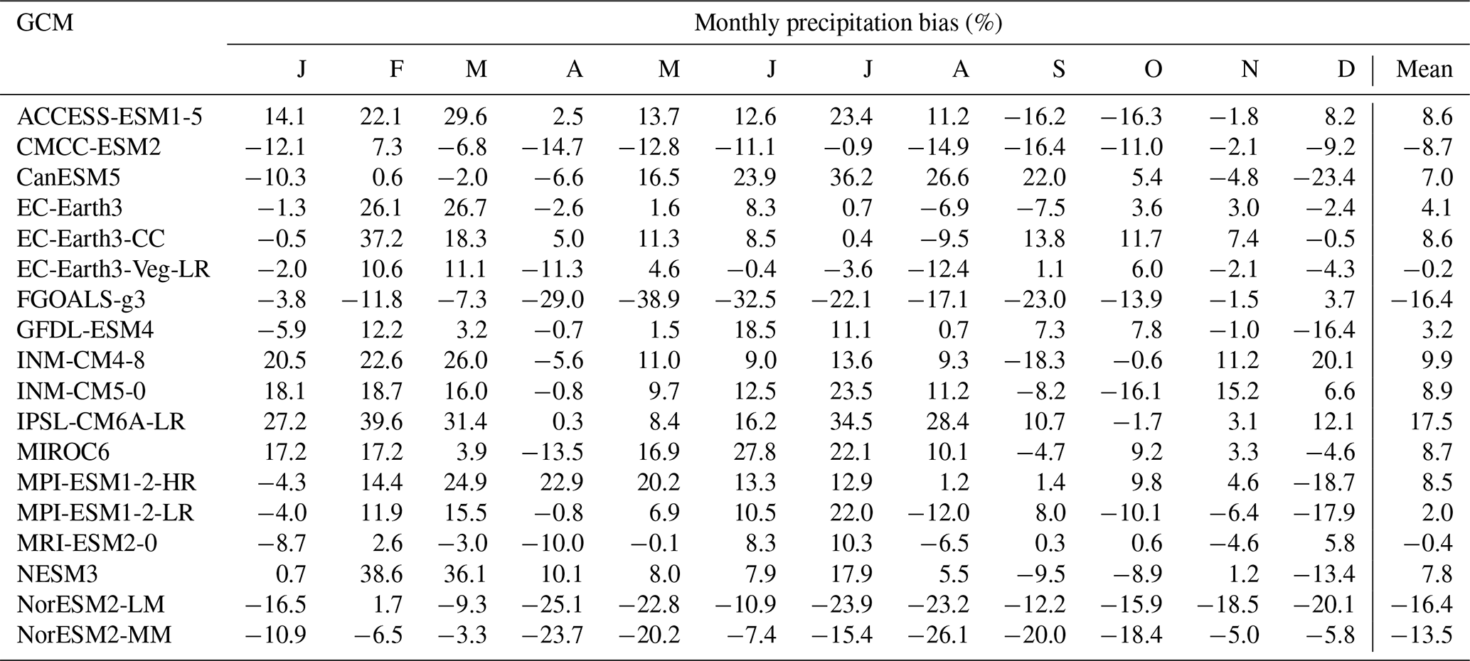
Table A3 Monthly temperature bias (°C) between 18 global climate models (GCMs) and ERA5 reanalysis data for the reference period (1981–2010). Values represent the average bias across the 10 catchments included in the study. Monthly biases are shown for January (J) through December (D), with the final column indicating the annual mean bias for each model.

Appendix B

Table B1 Kling-Gupta Efficiency (KGE) values for the conventional method during the calibration and validation periods across ten catchments. The mean KGE values for calibration and validation are also provided.

Table B2 Root Mean Square Error (RMSE) values calculated using sorted simulated and observed streamflow during the calibration and validation periods across ten catchments. The mean RMSE values for calibration and validation are also provided.

Appendix C: Appendix C

Figure C1 Performance comparison between the conventional, fully asynchronous and semi-asynchronous methods for the Bonaventure catchment during the reference period (1981–2010). The figure shows the percentage bias between observed and simulated streamflows, with the x-axis representing the observed daily streamflow and the y-axis displaying the percentage bias relative to the observed values. The shaded regions illustrate the variability among climate models around the mean bias for each method.

Figure C2 Same as Fig. C1, but for Ouelle catchment.

Figure C3 Same as Fig. C1, but for Bécancour catchment.

Figure C4 Same as Fig. C1, but for Nicolet Sud-Ouest catchment.

Figure C5 Same as Fig. C1, but for Au Saumon catchment.

Figure C6 Same as Fig. C1, but for Bras du Nord catchment.

Figure C7 Same as Fig. C1, but for Du Loup catchment.

Figure C8 Same as Fig. C1, but for Valin catchment.

Figure C9 Same as Fig. C1, but for Godbout catchment.

Appendix D

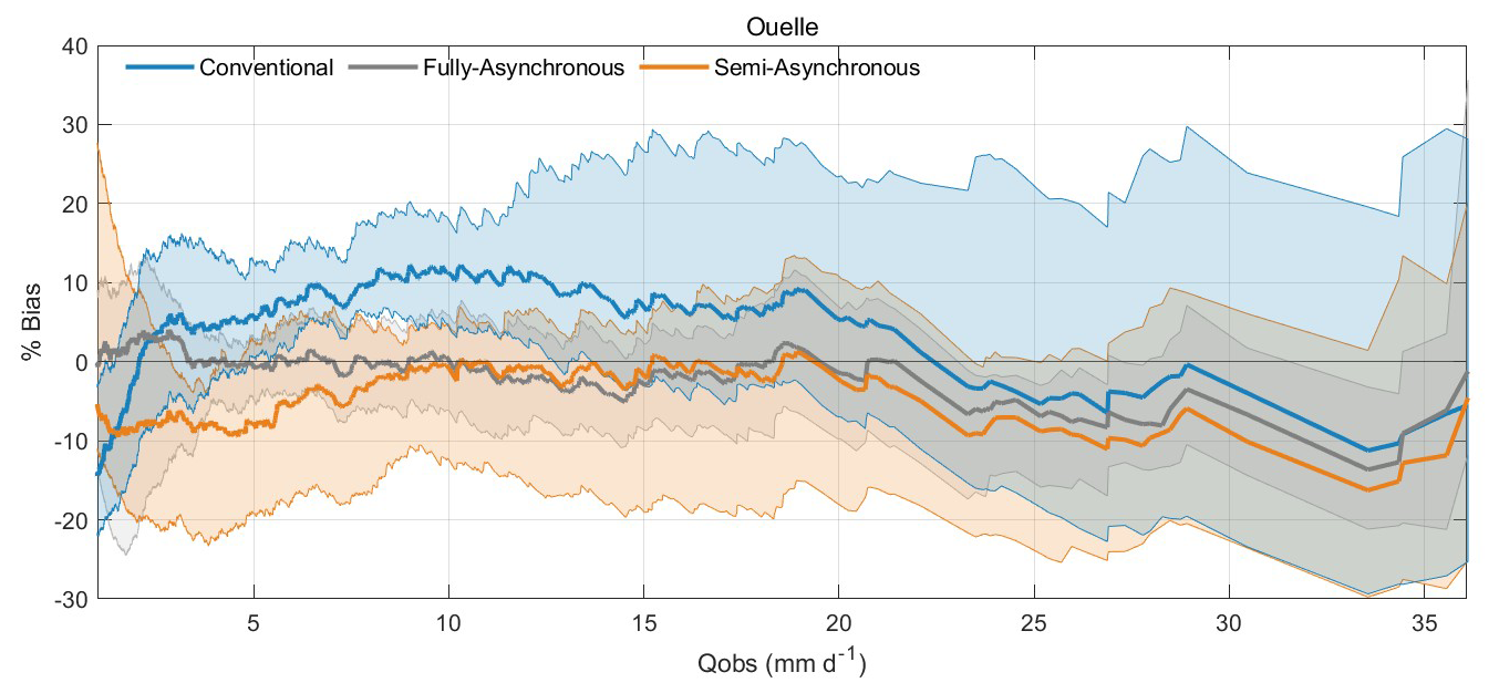
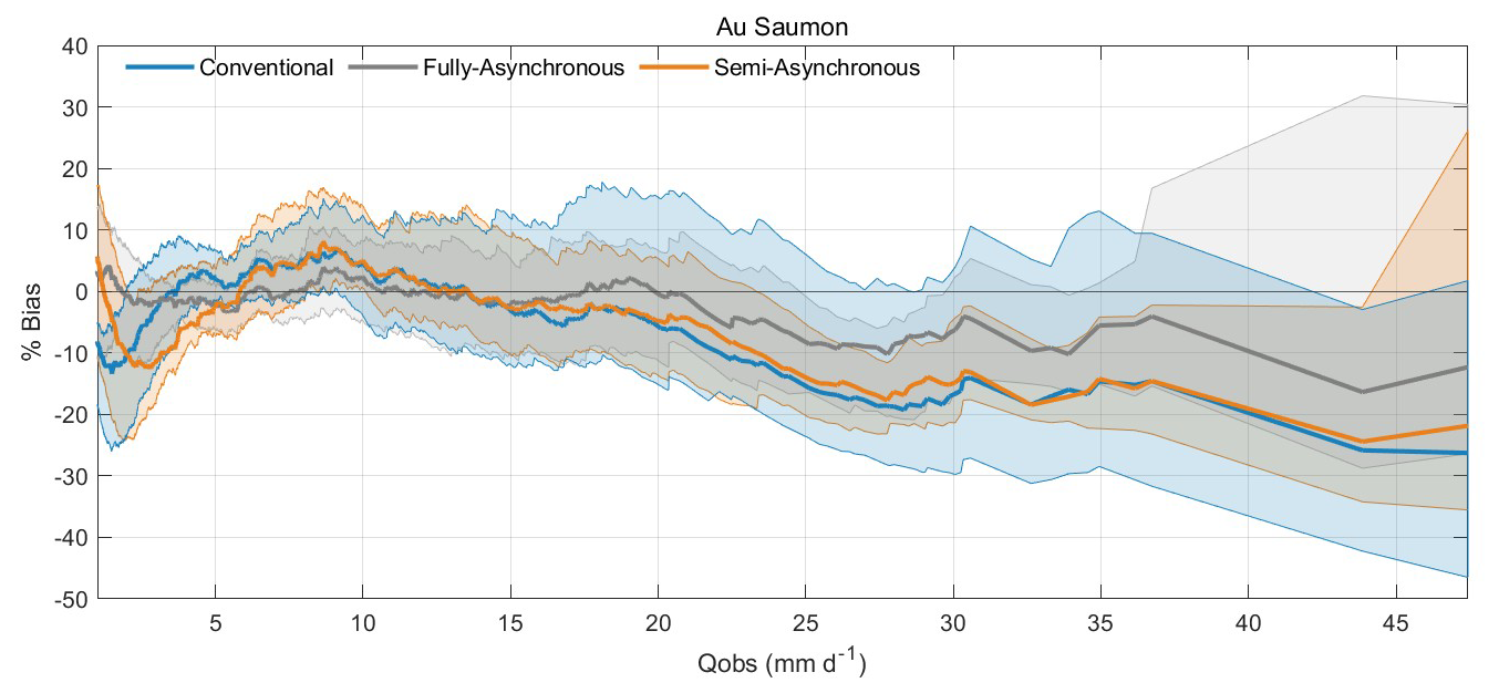
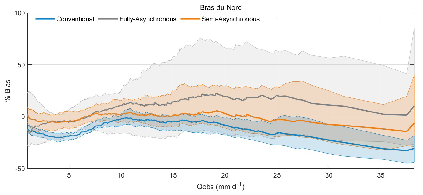
Table D1 Analysis of Q₉₅ % streamflow distribution across 10 catchments for the reference and future periods. Metrics include the median (med) and standard deviation (SD) of Q₉₅ % values (%).

Table D2 Same as D1, but for Q₅₀ %.

Table D3 Same as D1, but for Q₅ %.

Appendix E: Appendix E

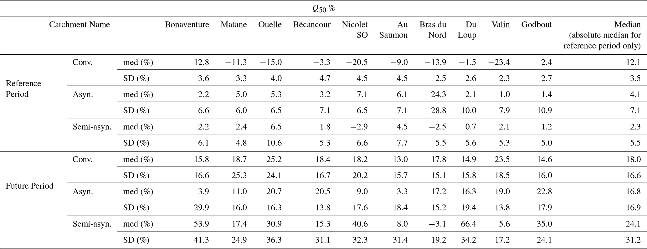
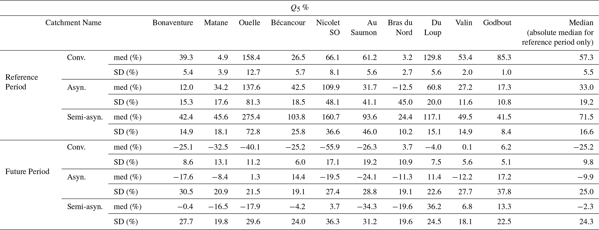
Figure E1 Seasonal distribution of key hydroclimatic variables for the reference period (1981–2010), future period (2070–2099), and their average absolute changes across the Bonaventure catchment.

Figure E2 Same as Fig. E1, but for Ouelle catchment.

Figure E3 Same as Fig. E1, but for Bécancour catchment.

Figure E4 Same as Fig. E1, but for Nicolet Sud-Ouest catchment.

Figure E5 Same as Fig. E1, but for Au Saumon catchment.

Figure E6 Same as Fig. E1, but for Bras du Nord catchment.

Figure E7 Same as Fig. E1, but for Du loup catchment.

Figure E8 Same as Fig. E1, but for Valin catchment.

Figure E9 Same as Fig. E1, but for Godbout catchment.

Appendix F: Appendix F

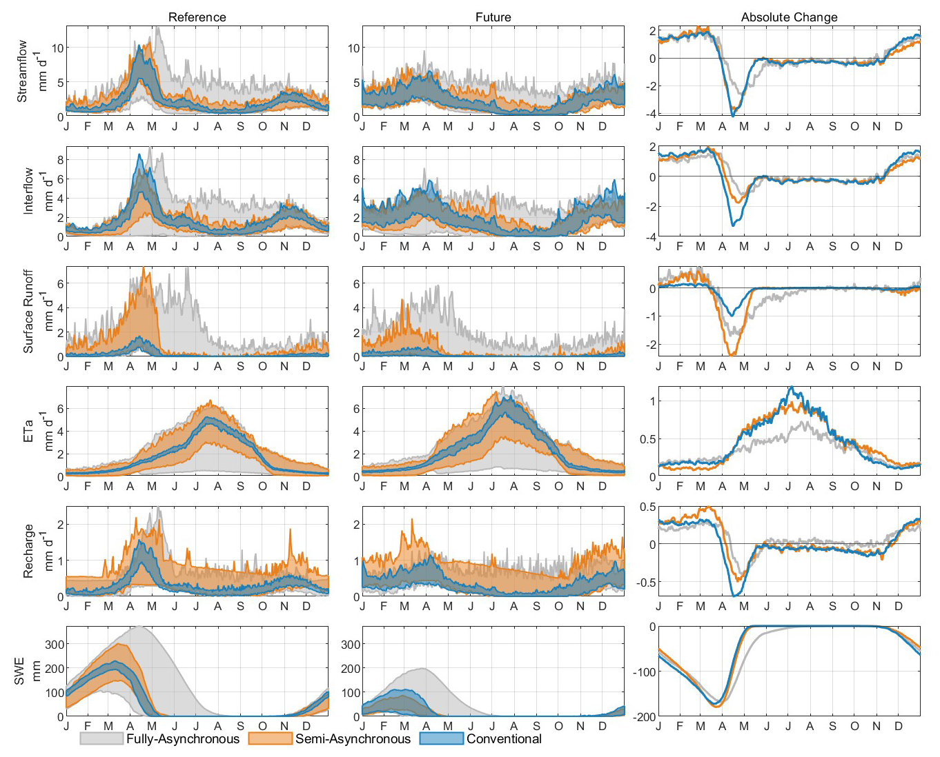
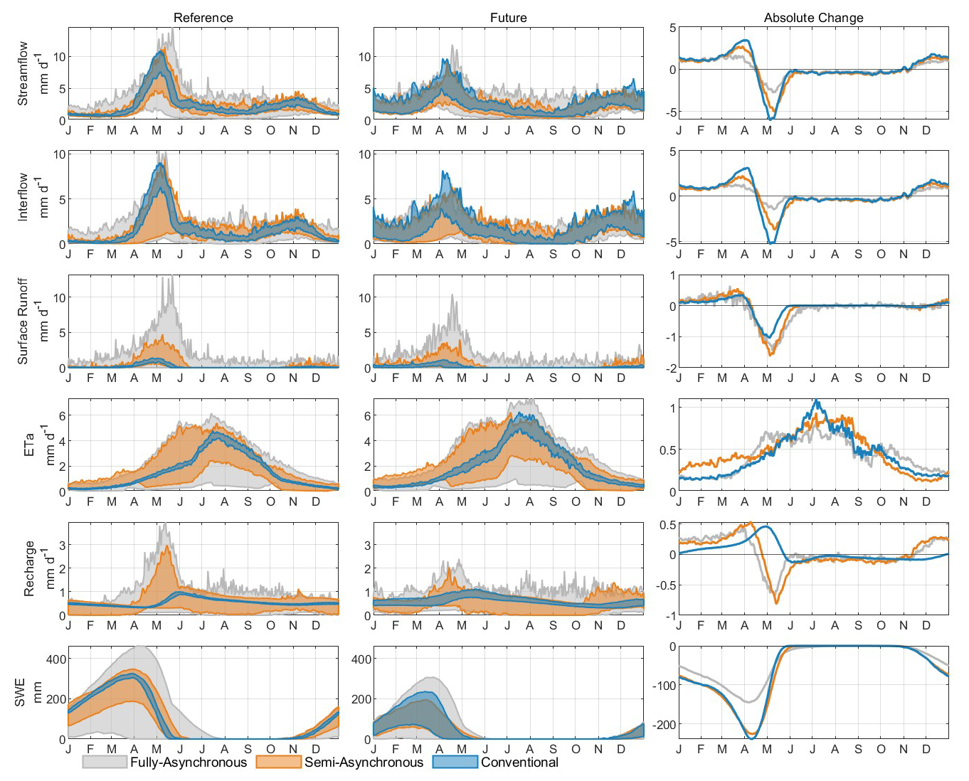
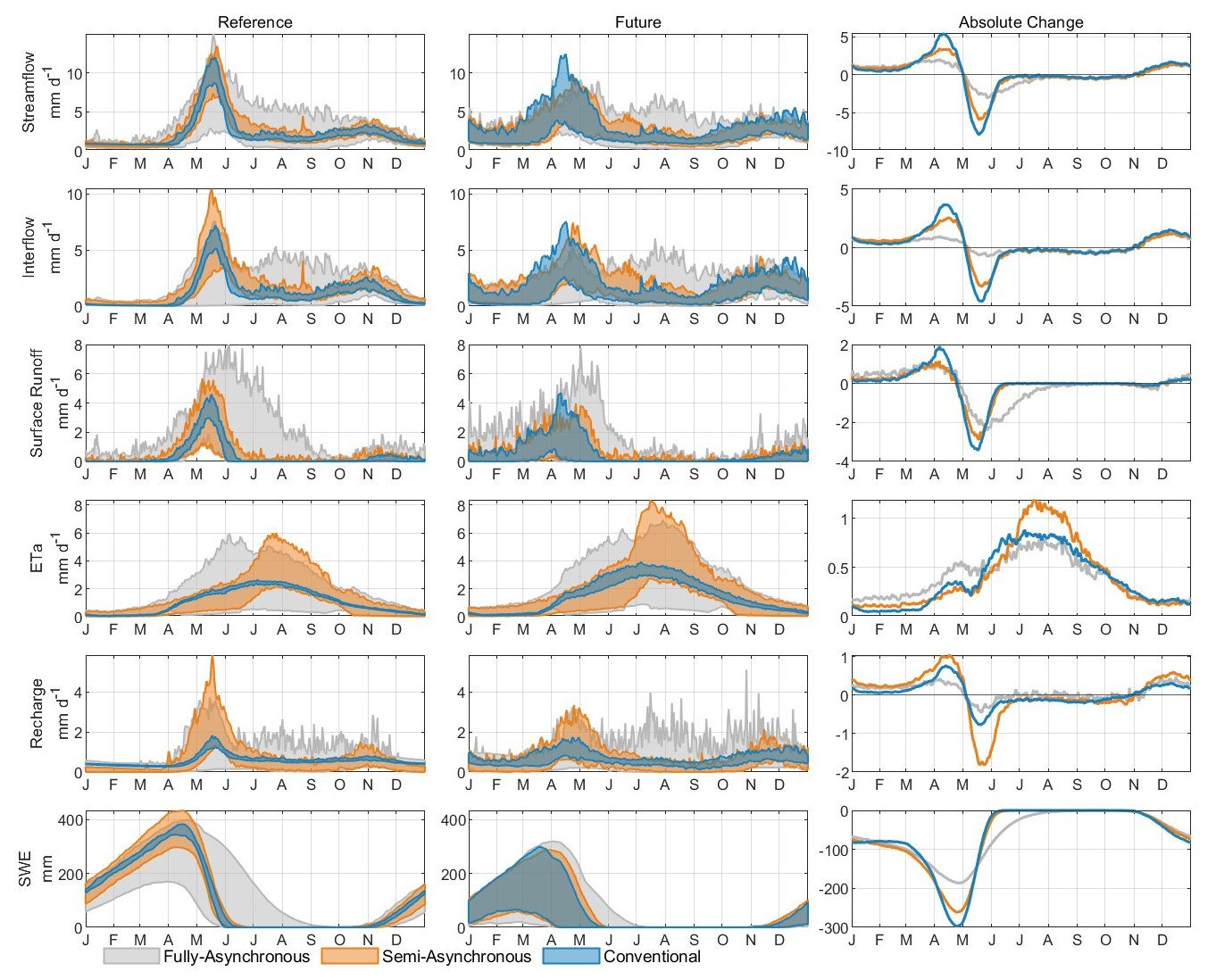
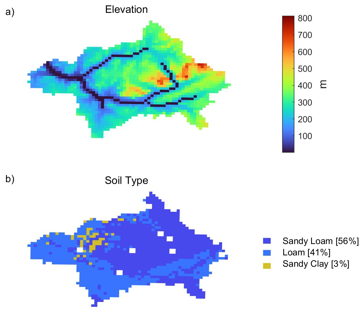
Figure F1 Topographic and soil type characteristics of the Matane catchment. Panel (a) shows the elevation map, with elevations ranging from 100 to 800 m above sea level. Higher elevations are indicated in warmer colors (reds and oranges), while lower elevations are shown in cooler colors (blues and greens). Panel (b) displays the distribution of soil types within the catchment, with sandy loam covering 56 % of the area (dark blue), loam covering 41 % (light blue), and sandy clay occupying 3 % (yellow).

Appendix G: Appendix G

Figure G1 Performance comparison between the conventional method calibrated using RMSE and KGE for the Matane catchment during the reference period (1981–2010). The figure shows the percentage bias between observed and simulated streamflows obtained using meteorological observations.

Figure G2 Seasonal streamflow comparison between the conventional method calibrated using RMSE and KGE and observed data across the Matane catchment.