Revealing the causes of groundwater level dynamics in seasonally frozen soil zones using interpretable deep learning models

Accurately characterizing groundwater level dynamics in seasonal frozen soil regions is of great significance for water resource management and ecosystem protection. To this end, this study proposes a new interpretable deep learning method to reveal the underlying causes of groundwater level dynamics on the basis of groundwater level simulation. Using the Songnen Plain in China as the study area and daily data from 138 monitoring wells, groundwater levels are simulated with an Long Short-Term Memory (LSTM) model, and the Expected Gradients (EG) method is employed to quantitatively identify the dominant factors and mechanisms of different groundwater level variation types.The results show that the LSTM model performs well on the test set, with the Nash-Sutcliffe Efficiency (NSE) exceeding 0.7 at 81.88 % of the monitoring sites, effectively capturing the temporal dynamics of groundwater levels. At the annual scale, three typical groundwater level variation types are identified: precipitation infiltration–evaporation type (29.0 %), precipitation infiltration–runoff type (18.1 %), and extraction type (52.9 %). Corresponding to the seasonal frozen-thaw period, groundwater level dynamics are classified into “V”-shaped (38.4 %), continuous decline (23.2 %), and continuous rise (38.4 %) types. Quantitative analysis using the EG method indicates that air temperature, precipitation, and snow thickness are the primary controlling factors of the “V”-shaped dynamics, reflecting the regulatory role of the frozen-thaw process on groundwater levels.When the initial groundwater level depth at the beginning of the freezing period is shallower than the sum of the frozen-thaw influence depth and the capillary rise height, a hydraulic connection is established between soil water and groundwater, resulting in typical “V”-shaped fluctuations. Conversely, when the depth exceeds this critical threshold, the frozen-thaw process cannot significantly influence the aquifer, and groundwater dynamics are mainly manifested as continuous rise or continuous decline, driven respectively by groundwater extraction and water level recovery following precipitation recharge. This study establishes an integrated framework of “simulation–classification–interpretation,” which not only improves the accuracy of groundwater level dynamic simulation and prediction but also provides new methods and perspectives for revealing the underlying mechanisms. The findings offer theoretical support and technical basis for regional groundwater resource management in cold regions.

1 Introduction

Groundwater level is a crucial indicator reflecting the water balance status of groundwater systems, and its dynamic changes reveal the evolving trends of regional hydrological processes. In terms of water resource management, monitoring groundwater level depth helps managers understand changes in groundwater storage, optimize water extraction schemes, and prevent resource depletion caused by overexploitation (Hao et al., 2014; Yang, 2012). Regarding ecosystem protection, fluctuations in groundwater level depth directly affect regional ecological patterns. Excessively low water levels may lead to wetland desiccation and biodiversity loss, while rapid rises can cause soil salinization and vegetation degradation (Singh et al., 2012). Relevant studies have also practically validated the significance of groundwater level prediction. For example, Liu et al. (2022) demonstrated in the lower Tarim River that machine learning–based groundwater level prediction models can quantitatively reveal current and future groundwater changes, clarifying the critical role of “ecological water conveyance” in regional ecological restoration. Therefore, in-depth identification of the controlling mechanisms behind groundwater level depth variations and achieving high-precision spatiotemporal simulation are of great significance for promoting sustainable groundwater resource utilization and ecological environment protection (Yi et al., 2022).

Seasonally frozen soil areas are widely distributed globally. In China, they cover more than half of the total land area, mainly in the northwest and northeast regions where water scarcity is a prominent issue (Wang et al., 2019). Unlike non-frozen soils, seasonally frozen soil is a unique water–soil system that contains ice, and changes in the ice content are accompanied by the dynamic storage of liquid water and dynamic changes in heat (Wu et al., 2023). The movement and storage behavior of groundwater in these regions differ from those in warm, non-frozen areas (Ireson et al., 2013), as the freeze–thaw process results in more frequent interactions between soil water and groundwater (Daniel and Staricka, 2000; Lyu et al., 2022; Lyu et al., 2023; Miao et al., 2017). This leads to significant differences in the causes of groundwater level dynamics between the freeze–thaw and non-freeze–thaw periods in seasonally frozen soil areas, making it more challenging to accurately simulate the regional groundwater levels.

Current models used for simulating groundwater level dynamics can generally be categorized into two groups: physical models and machine learning models (Ao et al., 2021). Most physical models are based on hydrodynamic processes and water balance principles, and are capable of accurately representing the physical mechanisms of groundwater systems. Therefore, they possess irreplaceable advantages in characterizing groundwater flow and uncovering hydrological processes such as recharge, runoff, and discharge. However, in areas with complex geological structures or highly heterogeneous aquifer systems, the construction, parameter calibration, and validation of physical models typically require large amounts of high-resolution geological, hydrological, and hydraulic data. These requirements make physical modeling challenging to implement and time-consuming (Raghavendra and Deka, 2014). Hence, there are few simulation studies on regional-scale groundwater level dynamics in seasonally frozen soil areas. In comparison, machine learning models have demonstrated significant advantages in simulating groundwater levels. These models explore the nonlinear relationships between inputs (such as meteorological and topographic data) and outputs (groundwater level) without the need to consider internal physical mechanisms (Rajaee et al., 2019), nor do they require predefined parameters such as hydraulic characteristics or boundary conditions (Ao et al., 2021). Despite this, machine learning models typically outperform physical models in terms of simulation accuracy, particularly in medium-to-long-term simulation studies (Demissie et al., 2009; Ebrahimi and Rajaee, 2017; Fienen et al., 2016; Rahman et al., 2020). One of the most successful deep learning architectures for modeling dynamic hydrological variables is the long short-term memory (LSTM) network (Jing et al., 2023; Wu et al., 2021). The LSTM model, which is an improved version of the recurrent neural network (RNN), can more effectively capture long-term dependencies in time-series data (Hochreiter and Schmidhuber, 1997). In the seasonally frozen soil regions of Northwest China, 14 years of continuous groundwater level simulations have shown that the LSTM model can effectively handle long-term data and accurately simulate groundwater levels in seasonally frozen soil areas (Zhang et al., 2018).

Although numerous studies have demonstrated the accuracy and predictive power of data-driven models in hydrological fields, these models are essentially black boxes and cannot explicitly explain the underlying physical processes and mechanisms (Zhou and Zhang, 2023). To address this limitation, researchers have proposed various methods to interpret deep learning models. Two widely used methods in groundwater research are the expected gradient (EG) method (Jiang et al., 2022) and the Shapley additive explanations (SHAP) algorithm (Lundberg and Lee, 2017). The broad application of the SHAP method is mainly attributed to its ability to reveal, from a local perspective, the contribution of each input variable to the corresponding model output at each time step (Wang et al., 2022) and, from a global perspective, the overall influence of input variables on the model output over the entire simulation period (Liu et al., 2022; Niu et al., 2023). However, the limitation of the SHAP method is that its interpretation of input factors is static and independent, making it ineffective in capturing the complex interactions between groundwater levels and long-term recharge and discharge dynamics. In contrast, the EG method (Jiang et al., 2022) calculates the EG values of the input variables over a specified time range, allowing for a better quantification of the impact of dynamic input variables on output variables at a particular time. This capability theoretically makes the EG method advantageous in groundwater level simulations with dynamic characteristics, particularly in explaining the temporal effects of meteorological changes on groundwater level across different periods. Nevertheless, there are currently no dedicated studies on the use of the EG method to explain the causes of groundwater level dynamics, and its effectiveness in understanding the relatively complex mechanisms of groundwater level dynamics in seasonally frozen soil areas requires further validation.

In this study, the seasonally frozen soil area of the Songnen Plain in Northeastern China was taken as an example. Through an in-depth analysis of three years of continuous monitoring data from phreatic wells in this region, combined with meteorological, hydrological, and soil texture data, the LSTM model was used to simulate the groundwater level dynamics. The reverse interpretation technique, i.e., the EG method, was applied to explore the decision principles of the deep learning model in simulating water levels during the non-freeze–thaw and freeze–thaw periods, thus revealing the mechanisms behind groundwater level dynamics across different periods in seasonally frozen soil areas. The research findings can demonstrate and extend the application of interpretable deep learning models in the groundwater field, providing essential support for groundwater resource assessment and ecological environment protection in seasonally frozen soil areas.

2 Data and methodology

Figure 1 shows the workflow of this study, including three main steps. First, the LSTM model is used to establish a nonlinear relationship between meteorological factors, human activities, and groundwater level depths (Fig. 1a). The daily air temperature, precipitation, extraction volume, and snow depth were used as input variables to predict the groundwater level depths. Subsequently, the EG method (Jiang et al., 2022) was applied to the trained LSTM model to obtain the EG scores of the input factors at different time steps. The EG scores quantify the influence of the meteorological inputs (air temperature, precipitation, and snow depth) and human activities (extraction volume) on the groundwater level depths during the simulation process (Fig. 1b). Finally, the causes of groundwater level dynamics during the non-freeze–thaw and freeze–thaw periods in seasonally frozen soil areas were identified.

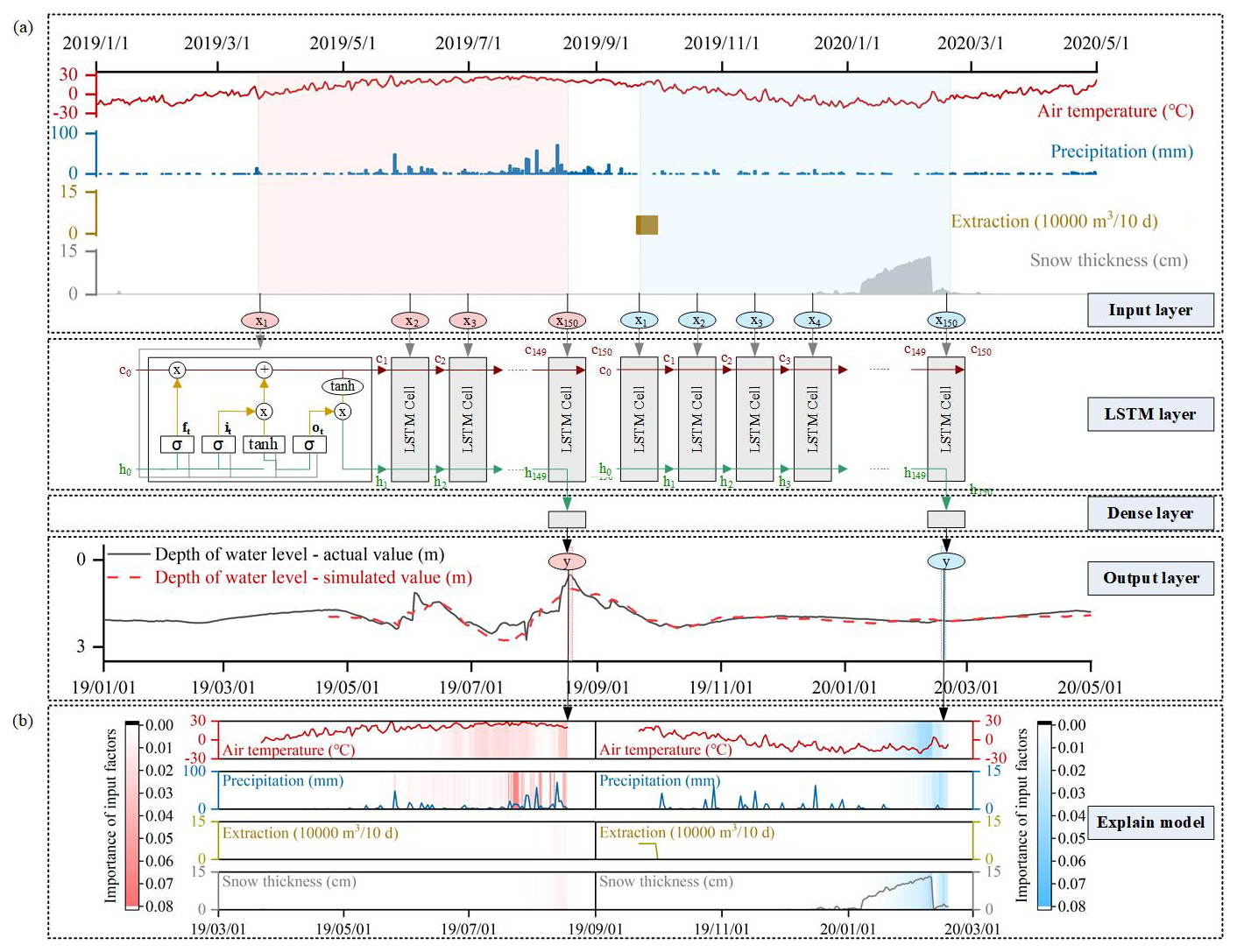
Figure 1 Workflow of this study: (a) Model structure of the LSTM model, (b) EG scores of input factors during the non-freeze–thaw and freeze–thaw periods.

2.1 Study area

The Songnen Plain is one of the three major plains in Northeast China. It is higher on the periphery and lower at the center, with a total area of 182 800 km² (Fig. 2a). The study area is surrounded by hills and mountains in the west, north, and east of the Greater and Lesser Xingan, Zhangguangcai, and Changbai Mountains, respectively, and is connected to the West Liaohe Plain by the micro-uplifted Songliao watershed in the south. The Songnen Plain primarily comprises the eastern high plain, western piedmont sloping plain, western low plain, and valley plain (Fig. 2a). The soil texture in the region mainly includes sandy loam, sandy clay loam, clay loam, and loamy clay (Fig. 2b). The climate in the area can be mainly characterized by two main types: first, it features a typical East Asian continental monsoon climate with hot, rainy summers and cold, dry winters; second, although the distribution of the climatic factors in the Songnen Plain is significantly influenced by latitude, there is a distinct east–west difference, with arid conditions in the west and humid conditions in the east (Li et al., 2022). The long-term average temperature of the Songnen Plain is 3.8 °C, the long-term average precipitation is 484.57 mm, and the long-term average evaporation is 1498.1 mm. The frost-free period ranges from 115 to 160 d. Freezing starts in mid-October from north to south, and thawing begins in April from south to north. The freezing depth ranges from 1.5 to 2.4 m (Zhao et al., 2009). The area is crisscrossed by rivers, with the Songhua River, Nenjiang River, and their tributaries forming a centripetal drainage system. The lower reaches of the Nenjiang River and Taoer River, as well as the Second Songhua River, flow through the central plain from the north, west, and southeast, respectively. The aquifer system in the Songnen Plain, China, consists of multiple aquifers ranging from the Cretaceous, Paleogene, and Neogene to the Quaternary. Among them, the Quaternary aquifer, whose distribution range is slightly smaller than that of the Cretaceous aquifer, is the main groundwater exploitation layer in the region and the aquifer in which the groundwater studied in this paper is located (Fig. 2c).

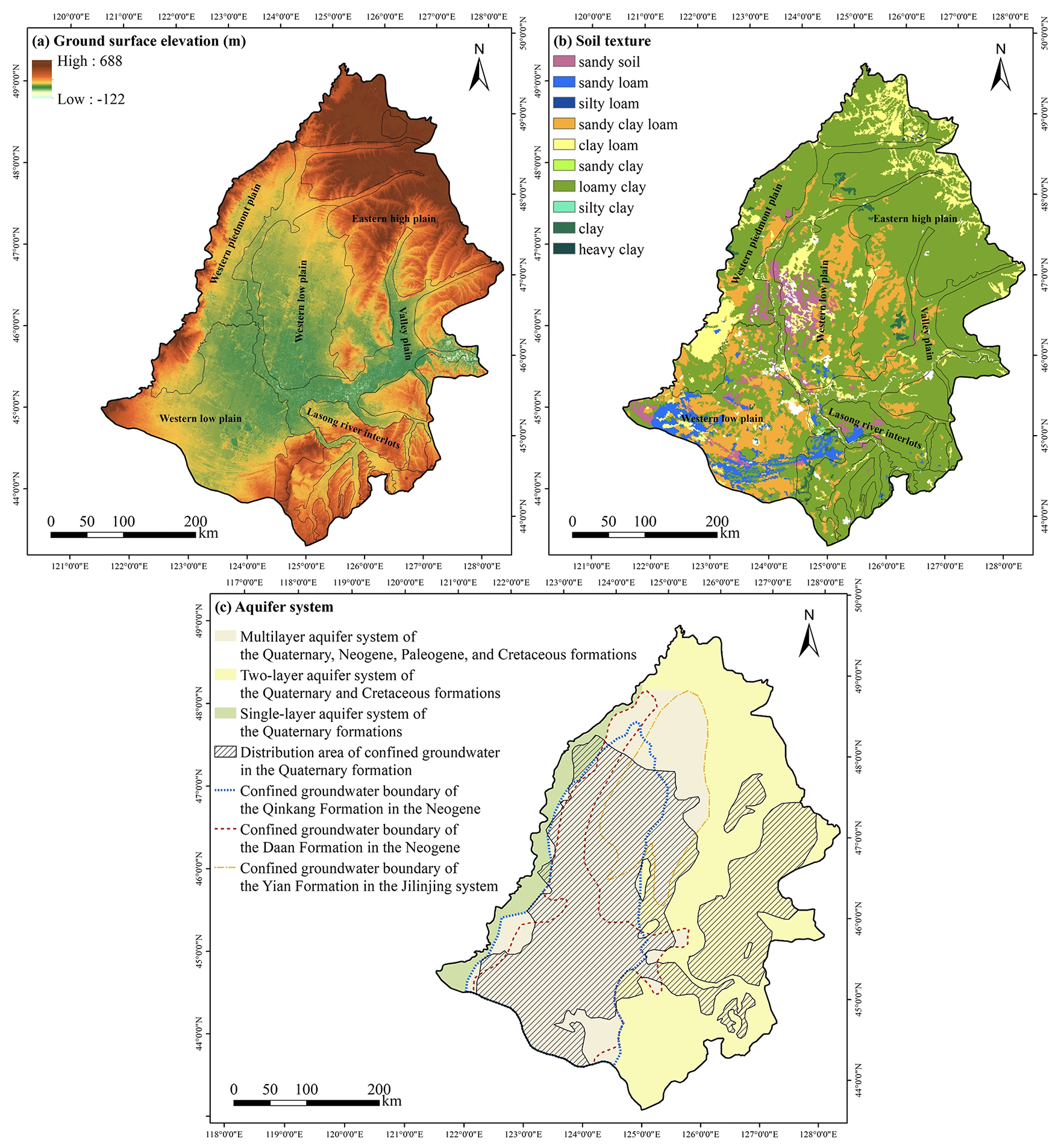
Figure 2 Spatial distribution of the ground surface elevation (a), topography (b) and aquifer system (c) in the Songnen Plain, China.

2.2 Dataset and selection of representative groundwater level values

To simulate the dynamic changes in the groundwater level in seasonally frozen soil areas and to analyze the driving mechanisms of groundwater level dynamics during freezing and non-freezing periods, this study primarily used dynamic observational data from 2018 to 2021, including precipitation, air temperature, snow depth, groundwater extraction volume, and groundwater levels, as well as static data such as ground surface elevation and soil texture. The precipitation and air temperature data were obtained from the “ERA5 hourly data on single levels from 1979 to present” dataset, provided by the European Centre for Medium-Range Weather Forecasts (ECMWF). ERA5 is the fifth-generation re-analysis of the global climate and weather data with a spatial resolution of 0.25° × 0.25° and an hourly temporal resolution. Daily snow depth data were sourced from the National Tibetan Plateau Data Center (https://data.tpdc.ac.cn/zh-hans/data/df40346a-0202-4ed2-bb07-b65dfcda9368, last access: 22 January 2026), with a spatial resolution of 25 km. The temporal and spatial resolution of the groundwater extraction volume data was enhanced based on the spatial distribution and water demand of major crops in the Songnen Plain, along with the precipitation data. Groundwater level data from 138 phreatic wells were provided by the China Geological Environment Monitoring Institute, while surface elevation data with a spatial resolution of 30 m were obtained from the Geospatial Data Cloud (https://www.gscloud.cn/search, last access: 22 January 2026). Soil texture data were sourced from the Resource and Environment Science and Data Center, compiled from a 1:1 000 000 soil type map and soil profile data collected during the second national soil survey of China.

In the Songnen Plain, approximately 70 % of groundwater extraction is used for agricultural irrigation; therefore, in this study, groundwater extraction was approximated based on crop water deficits. Using spatial distribution data of the region's major crops, 10 d period crop water requirements, and precipitation data, we estimated groundwater extraction at a fine resolution, ultimately generating 10 d period groundwater extraction data with a spatial resolution of 25 km × 25 km. Specifically, based on the water requirements of the main crops (rice, soybean, and maize), we calculated the total crop water demand for each 10 d period within each grid cell. These values were then weighted according to the crop planting area to obtain the total water demand per grid. By comparing precipitation with crop water demand, we determined whether precipitation could meet the crop water needs. When precipitation was sufficient, crops relied entirely on natural rainfall, and the effective precipitation equaled the water demand. When precipitation was insufficient, effective precipitation was limited by actual rainfall, and the remaining crop water deficit was assumed to be supplemented by other water sources. Finally, the difference between crop water demand and effective precipitation was calculated as the crop water deficit, which was assumed to be primarily supplied by groundwater. This allowed us to approximate 10 d period groundwater extraction. To ensure consistency with the temporal resolution of other variables used for model training, the 10 d period data were converted to daily averages by dividing by the number of days in each period.

To identify the causes of groundwater level dynamics during freezing and non-freezing periods, representative groundwater levels were selected for analysis using the EG method at different time periods. Based on the annual pattern of the groundwater level dynamics, groundwater levels during the non-freezing period are influenced by human activities, flood-season precipitation, and other factors, leading to greater fluctuations compared with that observed in the freezing period. Therefore, selecting extreme values (either maximum or minimum) as representative groundwater levels can effectively capture the peak or trough of the groundwater level, reflecting the most significant state of groundwater recharge or discharge during this period. Based on this, the trends in the groundwater level were analyzed to identify the different dynamic characteristics during the non-freezing period. If the groundwater level shows an overall uptrend, the maximum value represents the peak of the recharge process; if it shows a downtrend, the minimum value reflects the maximum extent of discharge.

However, during the freezing period, groundwater level fluctuations are relatively small, and extreme values do not respond significantly to external factors. During this period, groundwater levels may be influenced by soil freezing and thawing processes. Therefore, the groundwater levels at critical moments of soil freezing and thawing were chosen as representative values to more accurately reflect the response of groundwater level to environmental changes. During the freezing period, after the “Beginning of Winter” solar term (7–8 November), the average temperature continuously dropped to below 0 °C, and a thin ice layer gradually formed on the surface; after the “Rain Water” solar term (18–20 February), temperatures increased, and the frozen soil began to thaw in both directions; finally, the frozen soil fully thawed around the “Grain Rain” solar term (19–21 April) in spring (Lyu et al., 2023). Based on this climatic pattern, we uniformly defined the freezing and thawing periods for all monitoring wells in the study area. Specifically, the freezing period is defined as the interval from “Beginning of Winter” to “Rain Water,” and the thawing period as from “Rain Water” to “Grain Rain.” Therefore, the groundwater level at the “Rain Water” solar term was chosen as the representative groundwater level during the freezing period to capture the rapid response of the groundwater level to rising temperatures and thawing of the frozen soil.

2.3 Research methods

2.3.1 LSTM model

The LSTM neural network (Hochreiter and Schmidhuber, 1997) is an advanced RNN widely applied in deep learning. It can store and associate previous information, effectively addressing the issues of vanishing and exploding gradients that occur during the training of long sequence data. The deep learning model used in this study comprises a single LSTM layer and a dense layer. The LSTM layer is composed of recurrent cells arranged in a chain-like structure, allowing information to be passed from the current time step to the next. The model uses daily precipitation, air temperature, groundwater extraction volume, and snow depth from the previous 150 d as input sequences to predict groundwater level depths. Each cell in the LSTM layer includes four components: the input gate (i_t), the forget gate (f_t), the output gate (o_t), and the cell state (c_t) (as shown in the LSTM layer in Fig. 1a). The input gate determines how much input information is transferred to the cell state. The forget gate primarily controls how much information from the previous cell state is discarded and how much is carried forward to the current moment. The output gate calculates the output based on the updated cell state from the forget and input gates. The cell state is used to record the current input, the previous cell state, and the information from the gate structures. In this study, we adopted the LSTM equations proposed by Graves et al. (2013), which are represented by the following key equations:

$$\begin{array}{}\text{(1)}& {\displaystyle }{i}_t=\mathit{\sigma }\left(W_{xi}{x}_t+W_{hi}{h}_{t-\mathrm{1}}+b_t\right)\text{(2)}& {\displaystyle }{f}_t=\mathit{\sigma }\left(W_{xf}{x}_t+W_{hf}{h}_{t-\mathrm{1}}+b_f\right)\text{(3)}& {\displaystyle }{c}_t=f_t\odot c_{t-\mathrm{1}}+i_t\odot \tanh \left(W_{xc}{x}_t+W_{hc}{h}_{t-\mathrm{1}}+b_c\right)\text{(4)}& {\displaystyle }{o}_t=\mathit{\sigma }\left(W_{xo}{x}_t+W_{ho}{h}_{t-\mathrm{1}}+b_o\right)\text{(5)}& {\displaystyle }{h}_t=o_t\odot \tanh \left(c_t\right)\end{array}$$

where the input and output vectors of the implicit layer of the LSTM at time step t are x_t and h_t, respectively, the memory cell is c_t, and the values of the input, forget, and output gates are i_t, f_t, and o_t, respectively. W and b represent the learnable weight and bias terms to be estimated during the training period, respectively, σ(⋅) denotes the logistic sigmoid function, tanh(⋅) is the hyperbolic tangent function, and ⊙ represents elementwise multiplication.

Before training the model, the air temperature, precipitation, groundwater extraction volume, and snow depth were normalized by mapping their values to a range between 0 and 1. The adaptive moment estimation (Adam) algorithm (Kingma and Ba, 2015) was employed during training, with an initial learning rate set to 0.03. The maximum training epoch number was configured to 100, and an early stopping strategy was applied to prevent overfitting. For each individual groundwater monitoring well, 70 % of the input–output data pairs were randomly sampled for training the LSTM model, and they were split into training and validation samples at a ratio of 7:3. The training samples were repeatedly used to update the model parameters until the loss function for the validation samples ceased to decrease. The remaining 30 % of the data were used for an independent evaluation of the model performance. Random sampling allows for capturing the overall hydrometeorological variations observed across different time periods.

2.3.2 Model interpretations

In 2017, Sundararajan et al. (2017) developed the integrated gradients (IG) method, which uses the gradient of the model's output to the input factors to infer the specific contribution of the input variables to the output variable. The IG score for an input factor x (e.g., the precipitation at the ith time step), representing the degree of contribution of the input variable to the output variable, is expressed as follows:

$$\begin{array}{}\text{(6)}& {\mathrm{\varnothing }}_i^{\mathrm{IG}}\left(f,x,x^{\prime }\right)=\left(x_i-x_i^{\prime }\right)\underset{\mathit{\alpha }=\mathrm{0}}{\overset{\mathrm{1}}{\int }}{\displaystyle \frac{\partial f\left(x^{\prime }+\mathit{\alpha }\left(x-x^{\prime }\right)\right)}{\partial x_i}}\mathrm{d}\mathit{\alpha }\end{array}$$

where $\frac{\partial f\left(x^{\prime }+\mathit{\alpha }\left(x-x^{\prime }\right)\right)}{\partial x_i}$ denotes the local gradient of the network f at the interpolation point from the baseline input (x^′, when α=0) to the target input (x, when α=1).

However, the baseline input x^′ in the above formula is a hyperparameter that must be chosen carefully. In groundwater level studies, if the target input (e.g., a particular groundwater level observation) is close to the chosen baseline input (e.g., long-term average groundwater level), i.e., $x_i\approx x_i^{\prime }$, the IG method may fail to capture the importance of current input factors, such as precipitation or evaporation, on groundwater level changes (Sturmfels et al., 2020). To address this issue, Jiang et al. (2022) developed the EG method, which is based on the IG method but assumes that the baseline inputs follow the basic distribution D sampled from a background dataset (such as the training dataset), thus avoiding the need to specify a fixed baseline input. Given the baseline distribution D, the EG score ${\mathrm{\varnothing }}_i^{\mathrm{EG}}$ for the ith input factor can be calculated by integrating the gradients over all possible baseline inputs $x^{\prime }\in D$, weighted by the probability density function p_D. The EG score represents the influence of input factors on the model output, with a higher absolute EG score indicating a greater impact of the corresponding input factor on the model output, while an EG score close to zero suggests that the input factor has little effect on the output. The EG score can be expressed as follows:

$$\begin{array}{}\text{(7)}& {\mathrm{\varnothing }}_i^{\mathrm{EG}}\left(f,x\right)=\underset{x}{\overset{\prime }{\int }}\left({\mathrm{\varnothing }}_i^{\mathrm{IG}}\left(f,x,x^{\prime }\right)\times p_D\left(x^{\prime }\right)\mathrm{d}{x}^{\prime }\right)\end{array}$$

The above expression involves two integrals, which, according to Erion et al. (2021), can both be considered expectations. Thus, the equation can be reformulated as:

$$\begin{array}{}\text{(8)}& \begin{array}{rl}{\mathrm{\varnothing }}_i^{\mathrm{EG}}\left(f,x\right)& =E_{x^{\prime }\sim D,\mathit{\alpha }\sim U\left(\mathrm{0},\mathrm{1}\right)}\\ & \cdot \left[\left(x_i-x_i^{\prime }\right)\underset{\mathit{\alpha }=\mathrm{0}}{\overset{\mathrm{1}}{\int }}{\displaystyle \frac{\partial f\left(x^{\prime }+\mathit{\alpha }\left(x-x^{\prime }\right)\right)}{\partial x_i^{\prime }}}\right]\end{array}\end{array}$$

2.3.3 Evaluation metrics

The evaluation metrics used in this study include the Nash–Sutcliffe efficiency (NSE) coefficient and the root-mean-square error (RMSE). The NSE is used to assess the degree of fit of the regression model. The RMSE quantifies how well the predicted values match the observed values. If the NSE is close to 1 and the RMSE is close to 0, the model is more reliable.

$$\begin{array}{}\text{(9)}& {\displaystyle }\text{NSE}=\mathrm{1}-{\displaystyle \frac{{\sum }_{i=\mathrm{1}}^n{\left(x_i-y_i\right)}^{\mathrm{2}}}{{\sum }_{i=\mathrm{1}}^n{\left(x_i-\overline{x_i}\right)}^{\mathrm{2}}}}\text{(10)}& {\displaystyle }\text{RMSE}=\sqrt{{\displaystyle \frac{{\sum }_{i=\mathrm{1}}^n{\left(x_i-y_i\right)}^{\mathrm{2}}}{n}}}\end{array}$$

where x_i is the depth of the observed groundwater level, and $\overline{x_i}$ is the average value of x_i; y_i is the groundwater level depth simulated by the LSTM model; and i denotes the specific sample ordinal number, from 1 to n.

3 Results

3.1 Simulation Accuracy of Deep Learning Model for Groundwater Level

A data-driven model (LSTM model) was used to simulate the daily groundwater level depth of 138 aquifer monitoring wells in the Songnen Plain, China, from 2019 to 2021. Overall, the simulation accuracy of the groundwater level depth was relatively high across the western piedmont sloping plain, the eastern high plain, and the valley plain regions. In these areas, the NSE values at the monitoring points in the test set ranged from 0.53 to 0.96 (Fig. 3a), with 87.14 % of the monitoring points showing NSE values greater than 0.7. Over the entire simulation period (including the training and test sets), the maximum error between the simulated and observed values at each monitoring point mainly ranged from 0.5 to 2.5 m (Fig. 3b, d, and e), with 94.29 % of the monitoring points having an average error of less than 0.5 m. The annual groundwater level fluctuation at the monitoring points in this region was relatively small, ranging from 0.41 to 6.54 m.

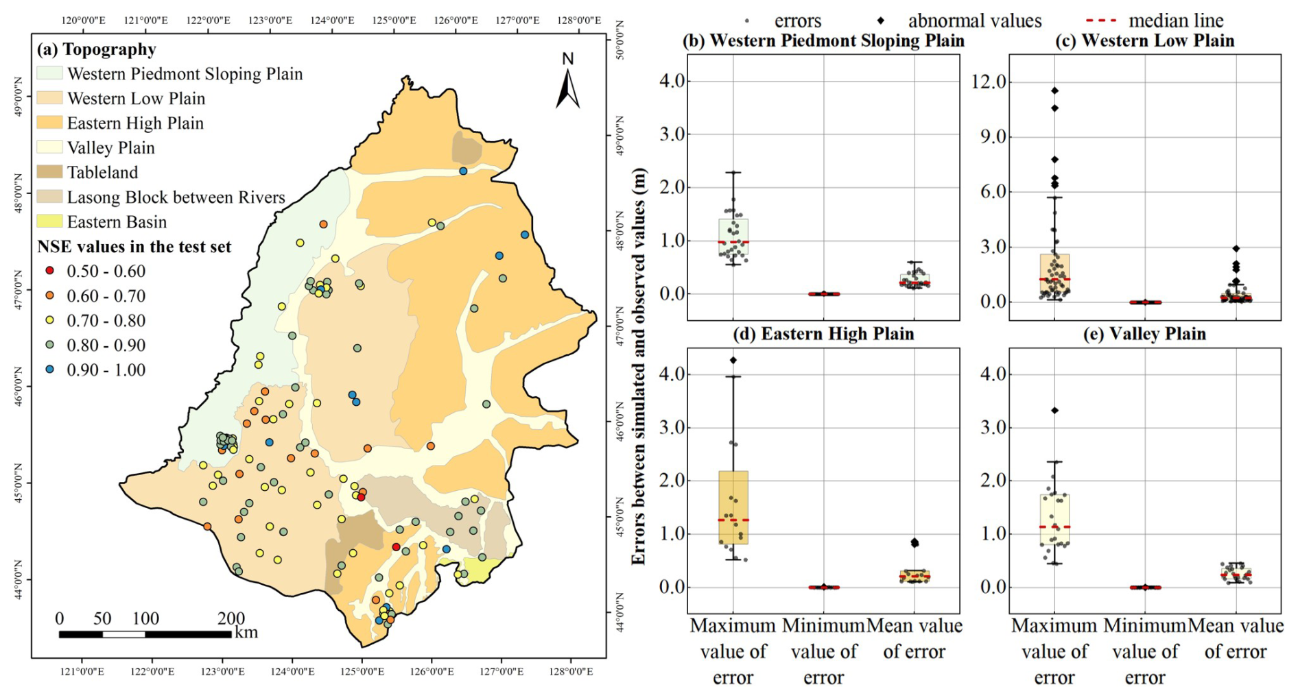
Figure 3 (a) Spatial distribution of the NSE values on the test set for 138 groundwater level monitoring points in the Songnen Plain, China. (b–e) Maximum, minimum, and mean errors between simulated and observed groundwater levels at monitoring points in the western piedmont sloping plain, western low plain, eastern high plain, and valley plain during the simulation period.

Only 18.11 % of the monitoring wells in the study area had a Nash-Sutcliffe Efficiency (NSE) below 0.7 on the test dataset, and these wells were primarily located in the southern part of the western low plain (Fig. 3a). In this region, the average absolute error between simulated and observed daily groundwater level depth ranged from 0.04 to 2.93 m, although the maximum error reached as high as 11.56 m (Fig. 3c), indicating that the model exhibited certain instability in localized areas. Figure 4 compares the simulated and observed groundwater level depth series at several poorly performing wells in this region. As shown in the figure, significant discrepancies occurred during certain periods, and the fitting performance was unsatisfactory. The primary reason for this discrepancy is the large annual fluctuation in groundwater level depth at many wells in this region: 21.43 % of the monitoring wells had a fluctuation range exceeding 10 m. These extreme fluctuations posed challenges for the LSTM model's simulation accuracy. In the training data used for the LSTM model, samples with extreme values of groundwater level depth were relatively scarce, while samples with moderate values were more abundant. Consequently, the model tended to fit the data in the moderate range more accurately, resulting in limited predictive ability for the extreme ends of the groundwater level series. Despite the reduced accuracy at certain wells, the LSTM model is capable of accurately capturing the variation trend of groundwater levels, and no significant lag is observed between the simulated and observed values (Fig. 4). The Pearson correlation coefficients between the simulated water levels and the measured water levels at the four representative monitoring points shown in the figure are 0.86, 0.81, 0.87, and 0.85, respectively. Moreover, the correlation coefficients reach their maximum values without applying any time lag, indicating that the simulated values can effectively and promptly reflect the actual variation trend of groundwater levels.

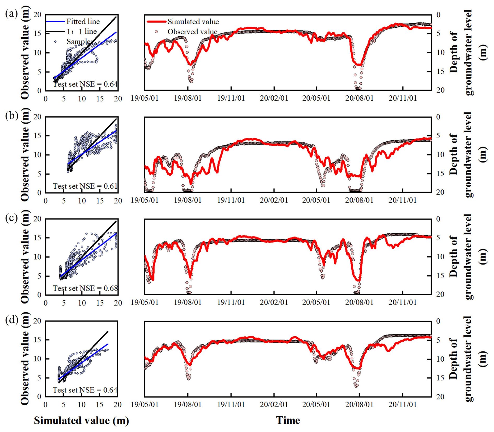
Figure 4 Comparison of the simulated and observed groundwater level depths at typical points in the western low plain (NSE values on the test set <0.7).

Overall, most of the groundwater monitoring points in the Songnen Plain, China, showed NSE values greater than 0.7 on the test set, indicating a relatively high simulation accuracy of the groundwater level depth based on the LSTM model. This suggests that the network structure of the LSTM model could accurately capture the dynamic relationships between the air temperature, precipitation, extraction volume, snow depth, and groundwater level.

3.2 Dynamic Characteristics of Regional Groundwater Level and their Distribution Laws

3.2.1 Annual Dynamics Variations and Spatial Distribution

Based on the characteristics of the annual groundwater level dynamic curves in the Songnen Plain, China, the annual groundwater level dynamics can be categorized into three types (Fig. 5).

The monitoring wells located in areas with a shallow groundwater level (less than 7 m) in the northern part of the western low plain and valley plain (Fig. 5a) exhibited annual groundwater level fluctuations of less than 4 m. Typically, the dynamic change in the groundwater level is as follows: during the dry season from January to April, precipitation is almost zero, and the groundwater level depth is significantly greater compared with those in the other months; with the onset of the rainy season (May to August), precipitation increases, causing the groundwater level to rise; after the rainy season ends (September to December), the groundwater level depth gradually increases with decreasing precipitation (Fig. 5b). This dynamic type of the groundwater level is the first annual dynamic type in the Songnen Plain, with its corresponding monitoring wells accounting for 29.0 % of all wells in the study area.

The monitoring wells located on Tableland, the Lasong Block between rivers, and the eastern high plain (Fig. 5a) have relatively greater groundwater level depths, ranging from approximately 5 to 11 m. From January to May each year, groundwater levels show a continuous decline; with the increase in precipitation, the groundwater level begins to gradually rise, reaching their annual peak in early October (Fig. 5c). The timing of the groundwater peak is delayed by 1 to 2 months compared with the first dynamic type, indicating that the response of the groundwater level to precipitation is slower (Fig. 5b and c). The annual groundwater level fluctuation is within 5 m. This dynamic type is the second annual dynamic type in the Songnen Plain, with its corresponding monitoring wells accounting for only 18.1 % of all wells in the study area.

In agricultural irrigation areas, such as the southern part of the western low plain and the western piedmont sloping plain (Fig. 5a), the groundwater level depth typically ranges from 5 to 20 m. The dynamic curves of the groundwater level in the aquifer monitoring wells in these areas exhibit distinct periodicity, showing a funnel-like and sawtooth pattern. The lowest groundwater levels typically occur in May or August, while the highest level typically occurs in November or later (Fig. 5d). During the irrigation season, groundwater levels drop significantly, with annual fluctuations being generally within 15 m. This dynamic groundwater type is widely distributed in the study area, with its corresponding monitoring wells accounting for 52.9 % of all wells, representing the third annual dynamic type in the Songnen Plain.

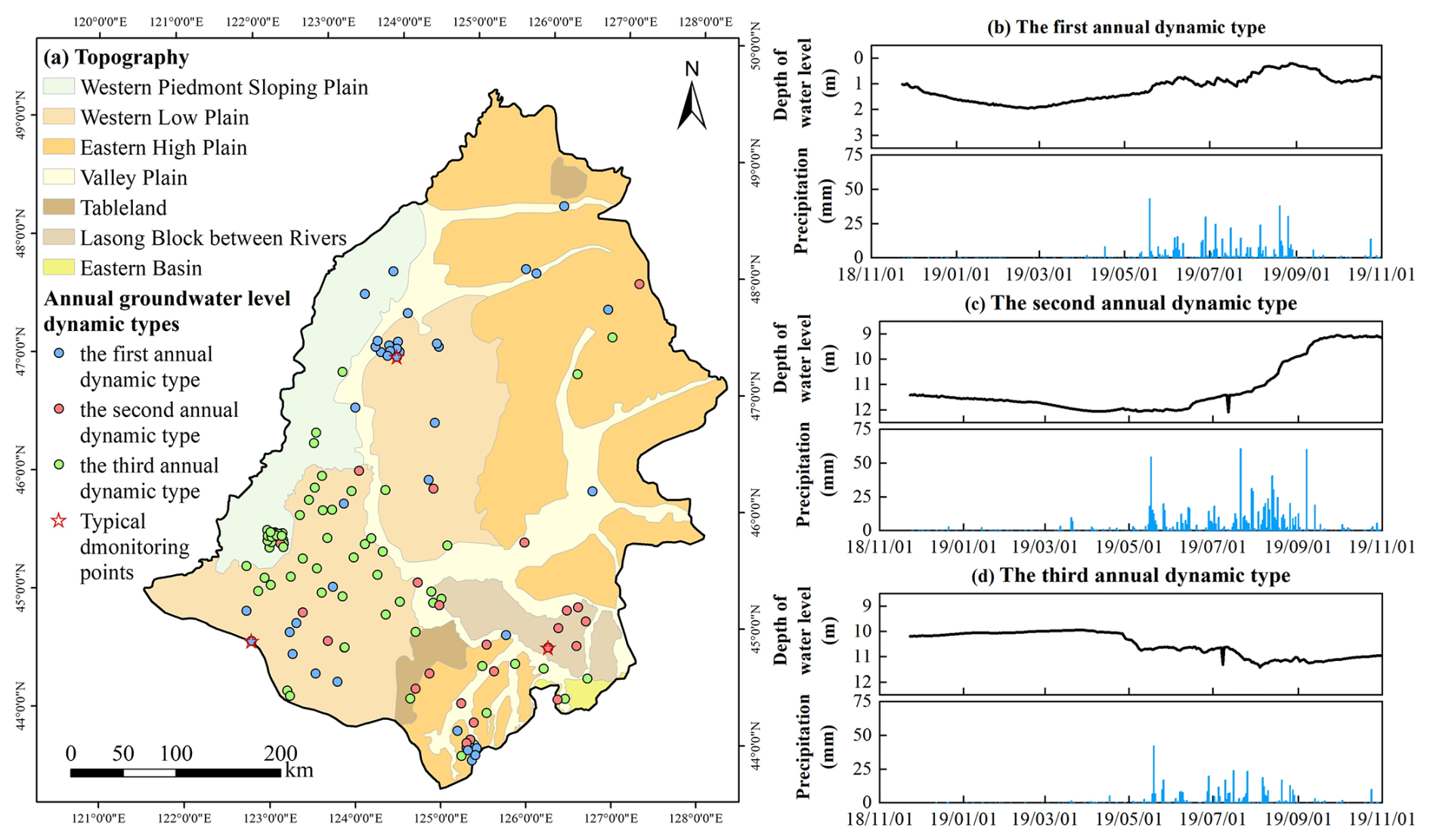
Figure 5 (a) Spatial distribution of different annual groundwater level dynamic types in the Songnen Plain, China; (b–d) Dynamic curves of different annual groundwater types and their corresponding precipitation variations. (b) The first annual dynamic type is represented by an unconfined aquifer monitoring well, numbered 230204210070, located in the western low plain; (c) The second annual dynamic type is represented by an unconfined aquifer monitoring well, numbered 220182210411, located in the Lasong Block between rivers; (d) The third annual dynamic type is represented by an unconfined aquifer monitoring well, numbered 220802210145, located in the western piedmont sloping plain.

3.2.2 Freeze–Thaw Period Dynamics Variations and Spatial Distribution

Freeze–thaw processes increase the frequency of interactions between soil water and groundwater (Daniel and Staricka, 2000; Lyu et al., 2022; Miao et al., 2017). As a typical seasonally frozen soil region, the Songnen Plain, China, exhibits three main forms of the dynamic curves of the groundwater level during the freeze–thaw period: “decline during freezing, rise during thawing,” “continuous decline,” and “continuous rise” (Fig. 6). The monitoring points of the different dynamic types during the freeze–thaw period accounted for 38.4 % (V-shaped), 23.2 % (continuous decline type) and 38.4 % (continuous rise type), respectively.

At monitoring points with a “V-shaped” groundwater level dynamic curve, characterized by “decline during freezing, rise during thawing” (Fig. 6a), the groundwater level fluctuated by approximately 0.2–0.9 m during the freeze–thaw period. The time when the groundwater level reached its maximum depth roughly coincided with the time when the soil reached its maximum frozen thickness. These monitoring wells are primarily distributed in areas with a shallow groundwater level in the northern part of the western low plain and the valley plain, with a few located in the southern part of the western low plain. At the beginning of the freezing period, groundwater level depths at these wells were typically within 5 m (Fig. 6d).

For the continuous decline and continuous rise types, the dynamic curves of the groundwater level during the freeze–thaw period exhibited either a “continuous decline” or “continuous rise” (Fig. 6b and c), with the rate of change remaining consistent throughout both the freezing and thawing periods. Monitoring points with the continuous decline in the groundwater level were mainly distributed in areas, such as the eastern high plain and the Lasong Block between rivers, where the groundwater level depth ranged from 4.52 to 11.51 m at the start of the freezing period (Fig. 6d). In contrast, monitoring wells with a continuous rise in the groundwater level during the freeze–thaw period were mainly found in agricultural irrigation areas such as the southern part of the western low plain and the western piedmont sloping plain, where the groundwater level depth at the beginning of the freezing period ranged from 4.71 to 19.91 m (Fig. 6d).

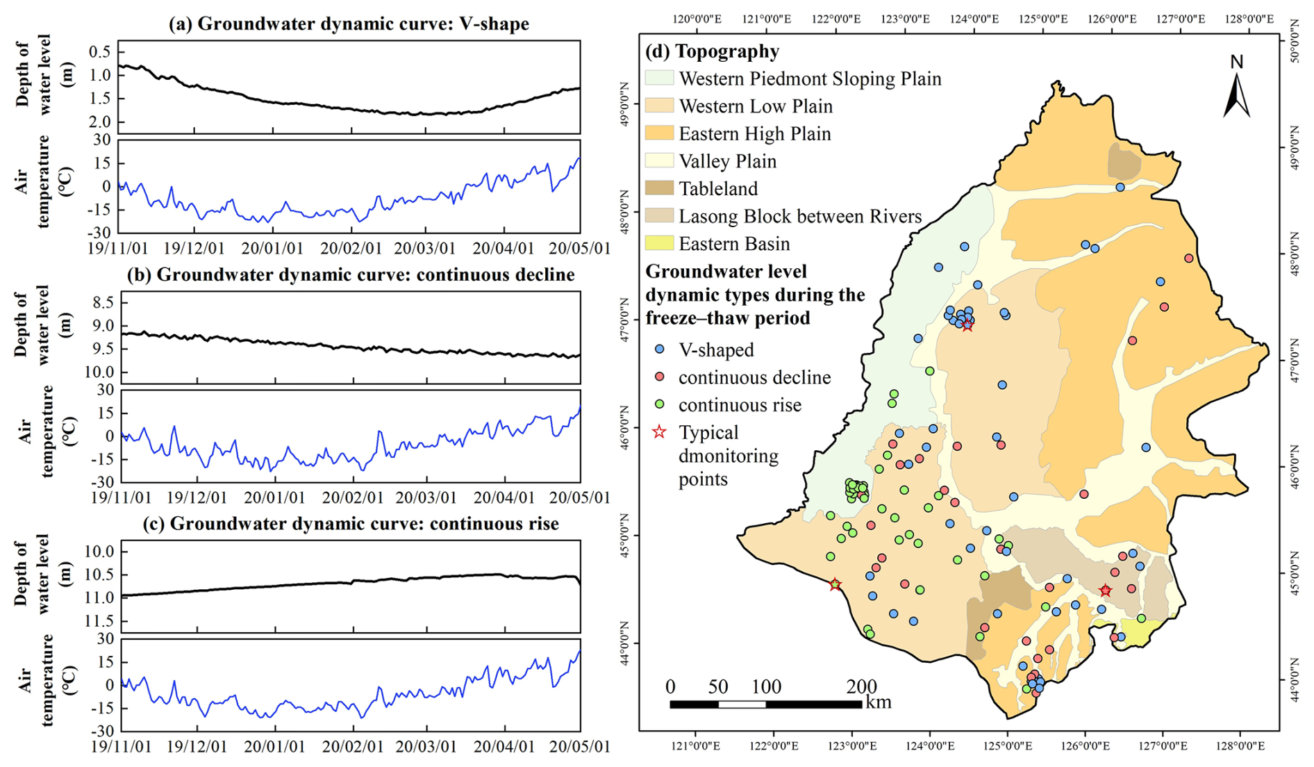
Figure 6 (a–c) Dynamic curves of different groundwater types during the freeze–thaw period and corresponding changes in air temperature; (d) Spatial distribution of different groundwater level dynamic types during the freeze–thaw period in the Songnen Plain, China. The dynamic curves of the groundwater level exhibiting patterns of (a) V-shaped, (b) continuous decline, and (c) continuous rise correspond to the unconfined aquifer monitoring wells numbered 230204210070, 220182210411, and 220802210145, respectively.

3.3 Main Controlling Factors and Identification of Causes for Various Groundwater Level Dynamic Types

After the application of the EG method to the trained models for the 138 groundwater level simulations, the EG scores (${\mathit{\varphi }}_i^{\mathrm{EG}}$) were obtained for precipitation, air temperature, extraction volume, and snow depth within 150 d prior to the representative groundwater level values for each annual and freeze–thaw period groundwater level dynamic type (Figs. 7 and 8).

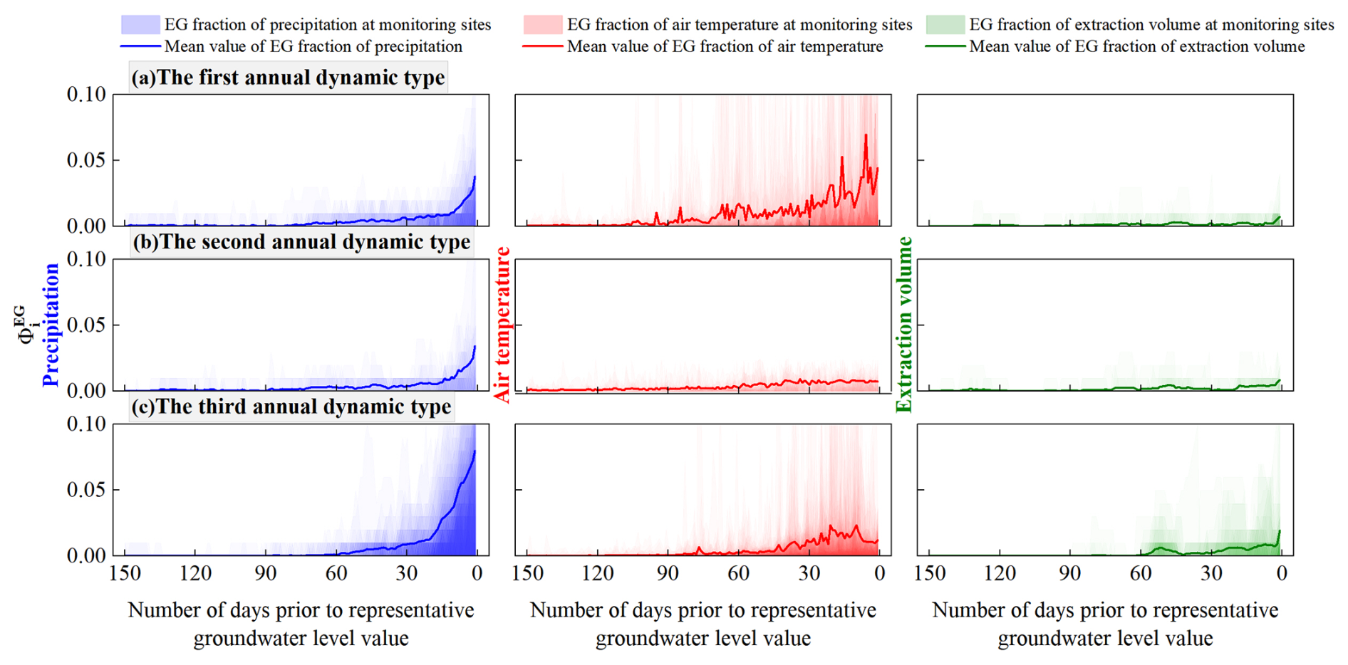
Figure 7 EG scores (${\mathit{\varphi }}_i^{\mathrm{EG}}$) of the precipitation, air temperature, and extraction volume for different annual groundwater level dynamic types in the study area at different time steps.

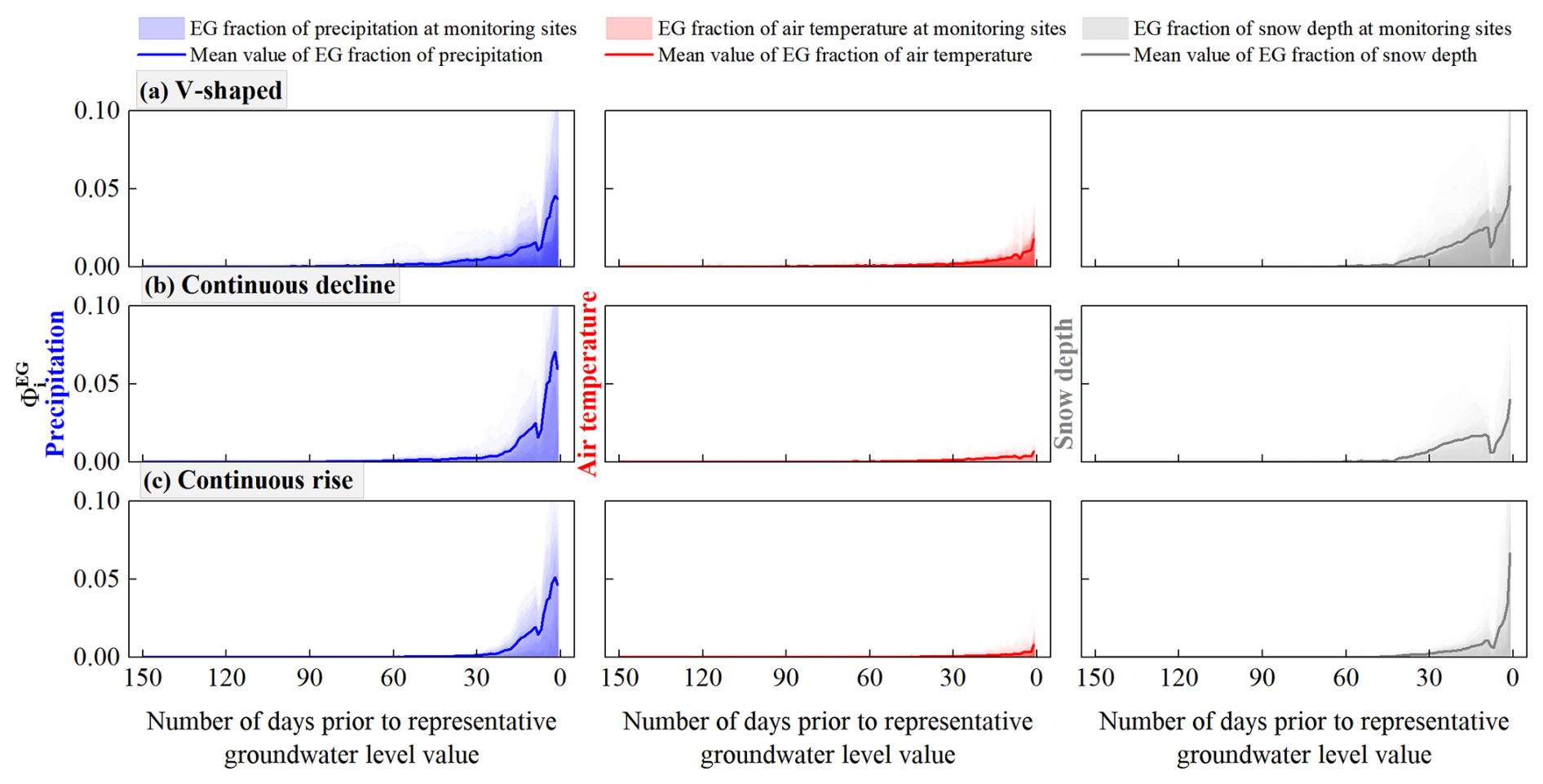
Figure 8 EG scores (${\mathit{\varphi }}_i^{\mathrm{EG}}$) of the precipitation, air temperature, and snow depth for different groundwater level dynamic types during the freeze–thaw period in the study area at different time steps.

3.3.1 Annual Dynamics: Influencing Factors and Dynamics Mechanisms

Within 90 d before the representative groundwater level values, the average EG scores for the precipitation and air temperature in the first annual dynamic type ranged from 0 to 0.04 and from 0 to 0.07, respectively, while the average EG score for the extraction volume did not exceed 0.01 (Fig. 7a). This indicates that the groundwater level depth in this dynamic type was significantly influenced by precipitation and air temperature, while the effect of extraction was negligible. Thus, the changes in the groundwater level depth may be related to the precipitation infiltration–evaporation process. When a pronounced precipitation peak occurred (Fig. 9b), the EG score increased significantly (exceeding 0.15), corresponding to a rise in groundwater level (Fig. 9e), indicating that precipitation infiltration made a substantial contribution to the groundwater level increase. Within the 90 d when precipitation influenced the representative groundwater level value, a total precipitation of 408.09 mm led to an overall rise in the groundwater level by 1.12 m (Fig. 9b and e). During periods without precipitation, the air temperature continued to rise (Fig. 9a), reflecting higher soil evaporation. At this time, the EG score for the air temperature was also relatively high (ranging from 0.10 to 0.20), and the groundwater level showed a slight decline (Fig. 9e). This suggests that evaporation was the primary discharge mechanism for groundwater in this dynamic type. Therefore, based on the groundwater recharge and discharge mechanisms, the first annual groundwater dynamic type is summarized as the precipitation infiltration–evaporation type.

In contrast, in the second annual dynamic type, only the precipitation had a significant impact on the groundwater level depth within 90 d before the representative groundwater level value (with the EG scores ranging from 0 to 0.03), while the average EG scores for the air temperature and extraction volume remained between 0 and 0.01 (Fig. 7b). Precipitation almost consistently recharged the groundwater during the 90 d before the representative groundwater level values (with an average EG score of approximately 0.012), causing a gradual rise in the groundwater level (Fig. 9j). However, the rate of groundwater rise was relatively slow, with an average value of approximately 0.02 m d⁻¹. The air temperature fluctuated significantly over the 90 d period (Fig. 9f), ranging from 4.41 to 28.57 °C, but had no significant impact on the groundwater level (Fig. 9j). The EG score during periods of high temperatures was also below 0.01, indicating that evaporation had little effect on the groundwater level. There was some groundwater extraction in local areas around July and October (Fig. 9h); however, it had a minimal impact on the groundwater level, with the EG scores remaining below 0.01. The relatively deep groundwater level (nearly 13 m) suggests that this groundwater type was primarily discharged through runoff. Therefore, the second annual groundwater dynamic type was classified as the precipitation infiltration–runoff type.

In the third annual dynamic type, the precipitation, air temperature, and extraction volume had a significant impact on groundwater level within a shorter period before the representative groundwater level values (within 60 d), with the average EG scores in the ranges of 0–0.08, 0–0.02, and 0–0.02, respectively (Fig. 7c). This dynamic type is mainly distributed in agricultural irrigation areas, such as the southern part of the western low plain and the western piedmont sloping plain (Fig. 5a). The main crops in these areas are rice, soybeans, and corn (You et al., 2021), and their water demand is concentrated in the summer, particularly between June and August (Xing et al., 2022). During this period, the air temperature shows a fluctuating uptrend (Fig. 9k), with the EG scores reaching a maximum of 0.02, indicating that high temperatures increase soil evaporation and crop transpiration. This leads to a higher water demand from the crops; however, the low rainfall was insufficient to meet this demand during these periods (Fig. 9l, with a daily maximum precipitation of only 33.80 mm), necessitating additional groundwater extraction for irrigation to maintain crop growth (Fig. 9m). As a result, the EG score for the extraction volume reached approximately 0.20 during this period, and groundwater level decreased accordingly (Fig. 9o). This dynamic type indicates that groundwater recharge comes from precipitation infiltration, and groundwater extraction is the main discharge mechanism. Thus, the third annual groundwater dynamic type was classified as the extraction type.

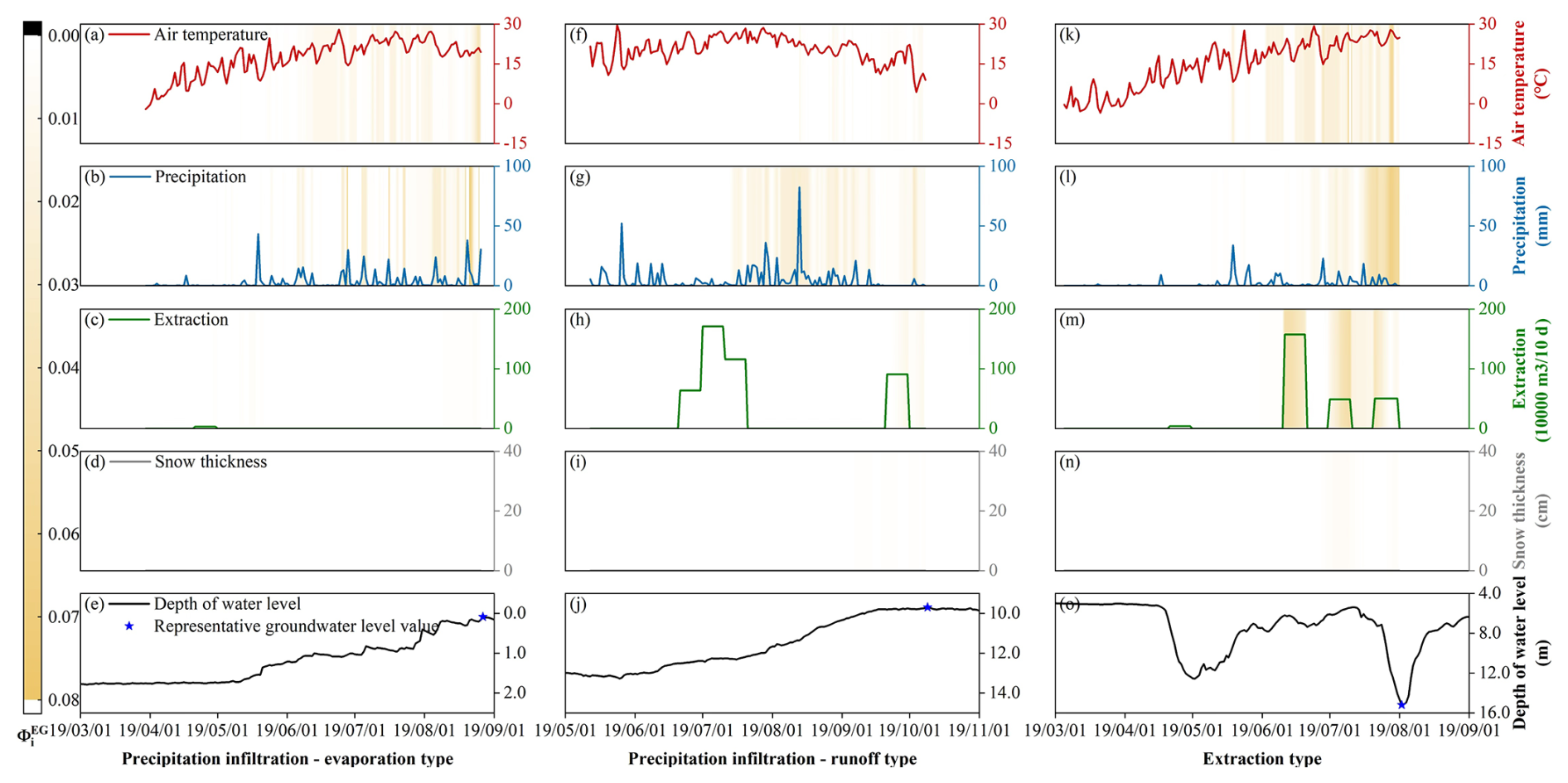
Figure 9 Observed values and EG scores (${\mathit{\varphi }}_i^{\mathrm{EG}}$) of the precipitation, air temperature, extraction volume, and snow depth within 150 d before the representative groundwater level values for various annual groundwater level dynamic types, as well as the corresponding annual groundwater level depth dynamic curves. The precipitation infiltration–evaporation type, precipitation infiltration–runoff type, and extraction type are represented by monitoring wells 230204210072, 220183210399, and 220821210024, with representative groundwater level values corresponding to 27 August 2019, 9 October 2019, and 2 August 2019, respectively.

3.3.2 Freeze–Thaw Dynamics: Influencing Factors and Dynamics Mechanisms

A further analysis focused on the groundwater dynamic types during the freeze–thaw period. In the V-shaped dynamic type, the average EG scores for precipitation and snow depth within 60 d before the representative groundwater level values ranged from 0 to 0.05, while the average EG score for the air temperature within 30 d before the representative groundwater level values ranged from 0 to 0.02 (Fig. 8a). This suggests that the air temperature, precipitation, and snow depth had a combined effect on the groundwater level depth of the V-shaped dynamic type during the freeze–thaw period. Within 30 d before the representative groundwater level values, the air temperature ranged from −21.10 to 4.40 °C, with the overall temperature being below 0 °C (Fig. 10b). As the air and soil temperatures dropped below 0 °C, the effective soil porosity decreased significantly due to water freezing, and the low-temperature suction related to the soil water potential between ice and water in the frozen soil increased gradually (Lyu et al., 2022). Under the combined effect of the capillary force and low-temperature suction, groundwater migrated upward continuously, thereby increasing the groundwater level depth (Fig. 10e). During this period, the snow depth increased with the decrease in temperature, reaching a maximum value of 13.22 cm on 9 February 2020 (Fig. 10d). The maximum EG score for the snow depth reached 0.03, indicating that snow had an impact on the groundwater level depth during the freeze–thaw period. When the air temperature exceeded 0 °C, the snow thawed rapidly (Fig. 10d), and the snow and frozen soil thaw water infiltrated to recharge the groundwater, causing the groundwater level to rise for the first time (Fig. 10e).

For the continuously declining and continuously rising dynamic types, only precipitation and snow depth affected the groundwater level depth during the freeze–thaw period. In the continuously declining groundwater dynamic type, the precipitation and snow depth influenced the groundwater level depth over a longer period before the representative groundwater level values (within 60 d), with the average EG scores below 0.07 and 0.04, respectively (Fig. 8b). In the continuously rising groundwater dynamic type, the average EG scores for the precipitation and snow depth within 30 d before the representative groundwater level values ranged from 0 to 0.05 and from 0 to 0.07, respectively, indicating that precipitation and snow depth affected the groundwater level depth in this dynamic type during the freeze–thaw period (Fig. 8c). Compared with precipitation and snow depth, the impact of the air temperature on the groundwater level in both dynamic types was negligible (Fig. 8b and c), with the average EG scores ranging from 0 to 0.01.

In both the freeze–thaw dynamic types, the air temperature fluctuated significantly over the past 150 d (Fig. 10f and k), whereas the EG scores remained below 0.01, indicating that the freeze–thaw effects had no significant impact on groundwater levels. Snow depth continued to increase during the winter when the air temperature was below 0 °C (Fig. 10i and n). When the air temperature rose above 0 °C, the snow gradually thawed, and the meltwater had some recharging effect on groundwater levels (with maximum EG scores reaching 0.04). However, due to the limited amount of snow and the high groundwater levels, the impact of snowmelt on the groundwater level was gradual and limited, failing to significantly alter the original trends in the continuously declining or continuously rising groundwater levels (Fig. 10j and o). Therefore, the causes of the continuously declining and continuously rising groundwater level dynamic types were related to the recovery process of the annual groundwater levels.

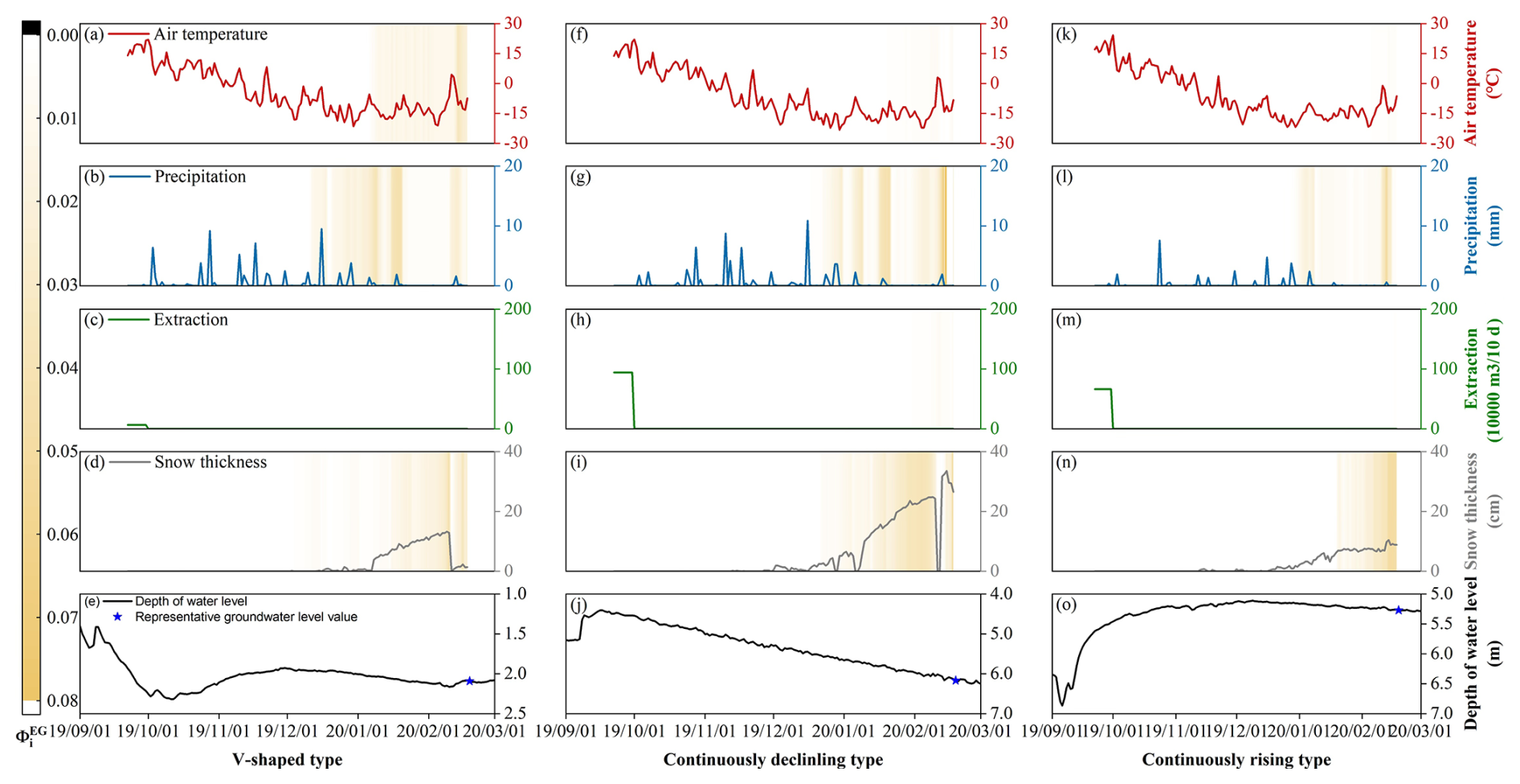
Figure 10 Observed values and EG scores (${\mathit{\varphi }}_i^{\mathrm{EG}}$) of the precipitation, air temperature, extraction volume, and snow depth within 150 d before the representative groundwater level values for various groundwater level dynamic types during the freeze–thaw period, as well as the corresponding annual groundwater level depth dynamic curves. The V-shaped, continuous decline, and continuous rise types are represented by monitoring wells 220106210371, 220182210410, and 220821210024, respectively. The representative groundwater level corresponds to 19 February 2020.

3.4 Regional Distribution Characteristics of the Dynamic Causes of Groundwater Level in the Songnen Plain, China

Based on the dynamic variations and spatial distribution characteristics of the groundwater levels in the study area, groundwater monitoring points where the groundwater levels dropped in the freezing period and rose in the thawing period, driven by soil freeze–thaw processes, typically showed a precipitation infiltration-evaporation dynamic in terms of the groundwater level dynamics during the year (Figs. 5b and 6a). These points were mainly distributed in areas with shallow groundwater level depths, such as the northern part of the western low plain and valley plain (Figs. 11a and 12a). Groundwater level dynamics unaffected by soil freeze–thaw processes generally showed two trends: continuous decline or continuous rise (Fig. 6b and c). Monitoring points with a continuous decline trend were mainly located in areas with a significant groundwater level depth, such as the eastern high plain and the Lasong Block between the rivers, where the annual groundwater level dynamics showed typical dynamic characteristics of precipitation infiltration–runoff type (Fig. 5c). The monitoring points in agricultural irrigation areas in the southern part of the western low plain and the western piedmont sloping plain showed a continuous rise in the groundwater level during the freeze–thaw period (Fig. 12a), and the dynamic type of the groundwater level in the year was mainly the extraction type (Fig. 5d). Therefore, the “continuous decline” groundwater dynamic during the freeze–thaw period was the recession phase of the groundwater level after the flood season peak in the precipitation infiltration–runoff-type groundwater, while the “continuous rise” groundwater dynamic was the recovery phase of the groundwater level after the extraction in the extraction-type groundwater.

However, under the classification based on the freeze–thaw period, the proportions of the V-shaped, continuous decline, and continuous rise types accounted for 38.4 %, 23.2 %, and 38.4 % of all monitoring points, respectively. These proportions did not completely align with the annual classification of the precipitation infiltration–evaporation (29.0 %), precipitation infiltration–runoff (18.1 %), and extraction (52.9 %) types. This discrepancy can be partly attributed to differences in the groundwater level depth. In some extraction monitoring points, although the annual groundwater level dynamics showed typical extraction characteristics, because the groundwater level at these monitoring points was shallow, the soil freezing and thawing processes still had a significant impact on it, resulting in a V-shape water level change at these points during the freeze–thaw period. The presence of such monitoring points increased the proportion of the V-shape type during the freeze–thaw period, while reducing the proportion of the continuous-rise type. Thus, the proportions of the freeze–thaw and annual classifications were not entirely consistent, particularly in areas with a shallow groundwater level depth, where soil freezing and thawing caused groundwater levels at some points of the extraction type to exhibit V-shaped variations during the freeze–thaw period.

In the northern part of the western low plain, where groundwater level was shallow (less than 5 m), the predominant annual groundwater dynamic was the precipitation infiltration-evaporation type (Fig. 11a). Due to the proximity of the groundwater level to the surface, the groundwater levels in these areas are more sensitive to meteorological factors. The dynamic curves of the groundwater level show a characteristic in that the high water level period corresponds to the rainy season. Specifically, in the Songnen Plain, peak precipitation and groundwater level in this dynamic type occur simultaneously, typically between July and August (Fig. 11d and f). The annual variation in the groundwater level was small, generally less than 4 m (Fig. 11c). During the freeze–thaw period, the groundwater level dynamics in this type exhibited a V-shaped pattern, with the groundwater level declining during the freezing period and rising during the thawing period, with a fluctuation range of 0.2–0.9 m. However, this V-shaped variation in the groundwater level is not accidental. At monitoring points with V-shaped dynamics, the initial groundwater level depth and soil freezing depth at the beginning of the freezing period were in the ranges of 0–5 m (Fig. 12d) and 1.6–2.1 m (Fig. 12c), respectively. The soil was predominantly silty clay, with a maximum capillary rise height of up to 5 m (Rui, 2004). Therefore, the initial groundwater level depth at these points was generally less than the sum of the soil freezing depth and the maximum capillary rise height (Fig. 12a). This means that during the freezing period, the low-temperature suction caused by soil freezing and the pre-existing capillary forces in the soil form a complete hydraulic connection between the frozen layer and the groundwater, causing the groundwater to continuously migrate toward the freezing front during the freezing period.

Groundwater monitoring points exhibiting the precipitation infiltration-runoff type were mainly distributed in the eastern high plain and the Lasong Block between rivers. In these areas, the groundwater level is deeper, typically ranging from 5 to 12 m (Fig. 11b), and runoff is the primary mode of groundwater discharge. The deeper groundwater level prolongs the infiltration time of precipitation, resulting in a delayed response of the groundwater level dynamics to precipitation recharge. Groundwater level peaks typically occur between August and October (Fig. 11d), lagging behind the precipitation peak by approximately one month (Fig. 11f). Due to the low recharge rate, groundwater level fluctuations are relatively moderate, with annual variations generally within 4 m (Fig. 11c). During the freeze–thaw period, groundwater monitoring points with continuously declining trends have greater initial groundwater level depths, ranging from 4.52 to 11.51 m at the beginning of the freezing period (Fig. 12d). This feature is primarily caused by the groundwater level rebound following the cessation of extraction after the irrigation period. With the cessation of agricultural water withdrawal, the depression cone formed by intensive extraction in the earlier stage begins to be replenished, and the groundwater level subsequently rises slowly. Due to the previously high extraction intensity and the relatively deep groundwater table, the recovery process does not occur instantaneously; instead, it is jointly constrained by the delayed response of the groundwater system and the regional recharge conditions. As a result, the groundwater level exhibits a steady and sustained upward trend. In addition, the soil freezing depth in this dynamic type was shallower (between 1.6 and 1.8 m), and the soil was still primarily silty clay (Fig. 12b and c). The greater groundwater level depth and shallower soil freezing depth prevented a complete hydraulic connection between the frozen soil and groundwater (Fig. 12a), resulting in the groundwater level being unaffected by the soil freeze–thaw process. Therefore, under conditions where no groundwater extraction occurs during the freeze–thaw period and the groundwater level is not influenced by freeze–thaw processes, the groundwater system continues the post-irrigation recovery process, presenting a “sustained rising” groundwater level pattern.

In the agricultural irrigation areas of the southern part of the western low plain and the western piedmont sloping plain, the groundwater level depth corresponding to the extraction types typically ranged from 5 to 20 m (Fig. 11b). During the agricultural irrigation period, significant groundwater extraction led to a marked decline in the groundwater level (Fig. 11c). The low groundwater level period coincided with the peak extraction period, typically between June and August (Fig. 11e and g). In areas with substantial groundwater extraction, a groundwater depression cone had already formed, with annual groundwater level fluctuations reaching up to 15 m (Fig. 11c). During the freeze–thaw period, the groundwater level dynamics exhibited a continuous rising trend. In the southern part of the western low plain and the western piedmont sloping plain, the initial groundwater level depth at the beginning of the freezing period and the soil freezing depth were in the ranges of 5–20 m (Fig. 12d) and 1.6–1.8 m (Fig. 12c), respectively, with the soil primarily comprising silty clay and sandy clay loam (with a maximum capillary rise height of 3 m) (Fig. 12b). In this region, the initial groundwater level depth was generally greater than the sum of the soil freezing depth and the maximum capillary rise height, causing the hydraulic connection between the vadose and saturated zones to be severed (Fig. 12a), and the groundwater level was unaffected by the soil freeze–thaw process.

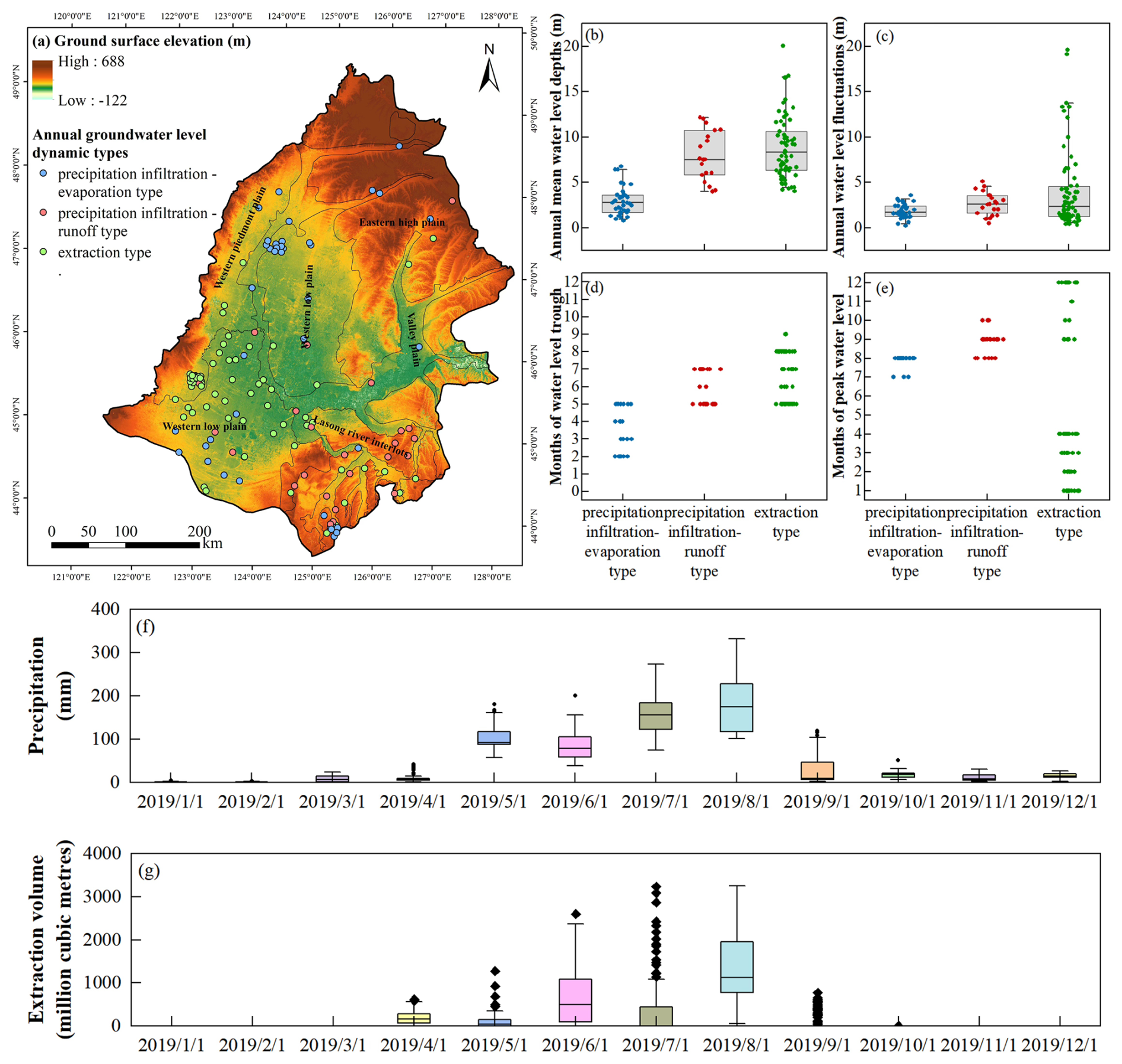
Figure 11 (a) Spatial distribution of the ground surface elevation and three dynamic types of annual groundwater level (precipitation infiltration-evaporation type, precipitation infiltration-runoff type, and extraction type) in Songnen Plain, China. The correlation between the three dynamic types of annual groundwater level and (b) annual mean groundwater level depths, (c) annual water level fluctuations, (d) months of peak water level and (e) months of water level trough. (f, g) Monthly distribution of the precipitation and extraction volume in Songnen Plain, China in 2019, respectively. Each point in (b)–(e) represents a groundwater level monitoring point.

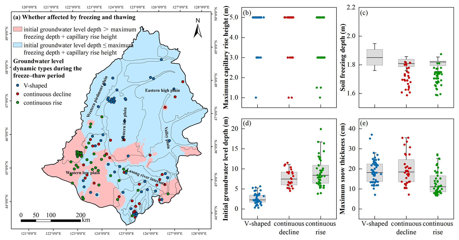
Figure 12 (a) Spatial distribution of whether the groundwater level is affected by the soil freeze–thaw process and the three groundwater level dynamic types during the freeze–thaw period (V-shaped, continuously declining, and continuously rising) in the Songnen Plain, China. Correlations between the groundwater level dynamic types in the three freeze–thaw period and (b) maximum capillary rise height of the soil, (c) the soil freezing depth, (d) the initial groundwater level depth at the start of the freezing period, and (e) maximum snow thickness. Each point in (b)–(e) represents a groundwater monitoring well.

4 Discussion

4.1 Implications of Groundwater Level Dynamics Classification for Water Resources Management

This study identified three main types of annual groundwater level dynamics in the Songnen Plain: the precipitation infiltration–evaporation type (29.0 %), the precipitation infiltration–runoff type (18.1 %), and the extraction type (52.9 %). This classification helps to reveal in greater depth the spatiotemporal distribution characteristics and response patterns of regional groundwater dynamics. Xu et al. (2024) demonstrated, based on random forest model analysis, that precipitation is the primary source of recharge for shallow groundwater in the Songnen Plain. This finding is consistent with the identification of the precipitation infiltration–type groundwater dynamics in this study, supporting the regulatory role of natural processes in groundwater levels. Meanwhile, Wu et al. (2025) reported that the significant groundwater decline in Jilin Province is mainly due to over-extraction for agricultural irrigation, particularly the large water demand associated with extensive rice cultivation. This observation echoes the finding that the extraction type accounts for the largest proportion of groundwater dynamics in this study, highlighting the substantial impact of human pumping activities on groundwater resources. On this basis, differentiated management strategies should be implemented for different groundwater dynamics types: in areas dominated by natural processes, ecological water requirements should be safeguarded and precipitation resources should be utilized comprehensively; in areas with significant human extraction, pumping schemes should be optimized to prevent ecological and social risks associated with excessive groundwater level decline.

During the freezing–thawing period, groundwater level dynamics are mainly divided into V-shaped type (38.4 %), continuously declining type (23.2 %), and continuously rising type (38.4 %), reflecting different response patterns of the groundwater system under the complex hydrological processes in seasonally frozen soil areas. Previous studies have indicated that soil freezing and thawing during the freezing–thawing period have significant impacts on groundwater recharge and discharge processes (e.g., Wang et al., 2023; Xie et al., 2021). The classification method adopted in this study, by identifying the overall dynamic characteristics during the freezing–thawing period, provides a more comprehensive description of groundwater response patterns. This classification not only facilitates accurate delineation of potential recharge and deficit zones in spring but also provides a theoretical basis for formulating differentiated water resources management strategies tailored to the freezing–thawing cycle, thereby enhancing the capacity to regulate groundwater dynamics in seasonally frozen soil areas.

4.2 A New Perspective on Identifying Groundwater Level Dynamics Mechanisms

Previous studies on the causes of groundwater level dynamics have generally relied on two main approaches. The first involves statistical methods such as trend analysis, correlation regression, or principal component analysis combined with the temporal variations of driving factors like precipitation, temperature, and water usage to infer potential dominant controls (Sarkhel et al., 2024). The second approach constructs numerical groundwater models or hydrogeological process-based models that quantify the influence of different drivers through parameter inversion, based on known aquifer structures, boundary conditions, and recharge-discharge processes (Petio et al., 2024). However, these methods face significant limitations when applied at the regional scale: statistical methods struggle to fully characterize complex nonlinear responses with multiple time lags and scales, while process-based models depend heavily on high-precision hydrogeological parameters that are often unavailable in most regions, and their results are susceptible to biases introduced by prior assumptions.

Differing from previous groundwater level dynamics research, this study explores the dominant factors and their mechanisms controlling various groundwater level changes in the Songnen Plain from the perspective of extracting information embedded within the LSTM model, thereby achieving a data-driven, bottom-up mechanism identification. This approach relies solely on multi-source observational data (precipitation, temperature, snow thickness, groundwater extraction, etc.) and can reveal the spatial (across monitoring wells) and temporal (intra-annual and seasonally frozen soil periods) patterns of dominant factor effects without requiring inaccessible hydrogeological data such as aquifer parameters and recharge-discharge relationships. Compared to traditional process-based models, this method not only enhances the feasibility and applicability of causative analysis but also reduces biases stemming from prior assumptions, providing a more realistic reflection of the groundwater system's response mechanisms (Jiang et al., 2022).

4.3 Limitations of existing models

A deep learning model was successfully developed in this study to simulate the groundwater level in the seasonally frozen ground regions of Northeast China, with 81.88 % of the monitoring wells in the study area achieving an NSE >0.7 on the test set. A common issue with deep learning models is that they are often considered black-box models, making it difficult to interpret their internal decision-making processes, which limits their credibility and interpretability in practical applications (Gunning et al., 2019). In groundwater level simulation studies, this research is the first to apply the EG method to quantify the importance of input factors in simulating groundwater level during non-freezing and freezing periods, revealing the driving forces behind groundwater level dynamics in different seasons. The introduction of this method offers a novel approach to understanding the groundwater level dynamics in seasonally frozen regions.

We opted for a local modeling approach (i.e., training a separate model for each groundwater monitoring well) rather than a regional approach (training a single model with data from multiple monitoring wells). This decision was based on our goal to identify the contribution patterns of the input factors (precipitation, air temperature, extraction volume, and snow depth) to groundwater level at the regional scale, including the duration of their influence and the significance of their impact. From a prediction standpoint, a regional model might be more suitable for areas where data are scarce or incomplete (Frame et al., 2022; Nearing et al., 2021), as it can learn more general relationships between input and output factors from historical data (Kratzert et al., 2019). However, regional models are associated with the issue of multicollinearity between static factors, and this issue must be addressed. Collinear input factors may share a substantial amount of information, making it difficult for the model to accurately distinguish the independent influence of each input factor on the output, leading to challenges in interpreting the impact of inputs on the output. Therefore, using regional models to explain the causes of groundwater level dynamics in seasonally frozen regions could be more challenging than using local models. Nevertheless, we acknowledge the advantages of regional models. Future research could further explore how to address the multicollinearity issues associated with static factors in regional models. In conclusion, we successfully combined deep learning models with the EG method to reveal the causes of groundwater level dynamics in seasonally frozen regions.

5 Conclusions

Groundwater dynamics in seasonally frozen regions are complex, influenced by both climate variability and human activities. Deep learning models require more sophisticated architectures and broader input variables to improve simulation accuracy, but this increases the difficulty of interpreting their internal mechanisms. Therefore, this study applies an interpretable deep learning approach to reveal the driving mechanisms behind groundwater level dynamics in seasonally frozen soil regions. High-precision simulations of groundwater levels at 138 monitoring points were conducted using an LSTM model, and combined with the EG method, the main controlling factors and underlying mechanisms of different types of water level changes were identified. The main findings are as follows:

First, the LSTM model demonstrated high accuracy in simulating groundwater level variations in seasonally frozen areas, with NSE values on the test set ranging from 0.53 to 0.96, indicating its effectiveness in capturing complex groundwater dynamics.

Second, by applying the EG method, three dominant intra-annual groundwater dynamic types in the Songnen Plain of China were identified: precipitation infiltration–evaporation type (29.0 %), precipitation infiltration–runoff type (18.1 %), and extraction type (52.9 %). Correspondingly, during the freeze–thaw period, these types are reflected as V-shaped, continuously declining, and continuously rising patterns, accounting for 38.4 %, 23.2 %, and 38.4 % of the monitoring wells, respectively.

Third, while all three intra-annual types are primarily recharged by precipitation infiltration, their discharge pathways differ: evaporation, runoff, and groundwater extraction, respectively. During the freeze–thaw period, changes in the soil water potential gradient due to freezing and thawing lead to interactions between soil water and groundwater, resulting in the V-shaped variation. In contrast, the continuously rising and types declining reflect gradual water level changes primarily driven by groundwater extraction and precipitation recharge, without strong influence from freeze–thaw processes. These dynamic types represent groundwater fluctuations jointly driven by multiple factors across different temporal scales.

The results demonstrate the great potential of the EG method to bridge model accuracy and interpretability, offering a new perspective for analyzing complex hydrological processes. Future research may incorporate more advanced interpretability techniques to further enhance understanding of deep learning models. The significance of deep learning lies not only in high-accuracy simulations, but also in advancing the discovery of hydrological mechanisms. This study provides new methodological support and theoretical insights for groundwater resource management in seasonally frozen soil regions.