Detection of compound and seesaw hydrometeorological extremes in New Zealand: A copula-based approach

Compound hot and dry and dry-to-wet seesaw events are hydrometeorological extremes that involve the propagation of water deficits through the hydrological cycle, driven by multiple interactions between precipitation, temperature and soil moisture. Here we demonstrate new understanding of such events gained by directly modelling these interactions using copulas rather than treating each variable separately. New Zealand makes for a useful case study, owing to the occurrence of relatively high-magnitude extremes across strong hydroclimatic gradients. Standardised indices are constructed for soil moisture, temperature and precipitation using ERA5-Land for 1950–2021. A conventional bivariate copula model is used to capture the joint variation between precipitation and soil moisture indices for seesaw events, with a trivariate (vine) copula used for modelling all three indices during compound events. Differences in compound event detection are strongest in eastern regions, where evapotranspiration is more important for dry phase development. The copula approach reveals more frequent/extreme occurrence of compound events compared to coincident extremes in separate variables: for a 1-in-100-year vine copula event the equivalent magnitude coincident soil moisture and temperature extreme is a 141-year event (171-year for the coincident precipitation-temperature event). Large differences in seesaw event detection also occur in the east: compared to a 1-in-100-year bivariate copula event the equivalent soil moisture extreme is less frequent (126 years) but the precipitation extreme more frequent (65 years). These results highlight the advances that a copula approach can provide in terms of better understanding the magnitude-frequency characteristics of compound and seesaw events, as well as their drivers – critically important for managing the impacts of these events, especially in the context of climate change.

1 Introduction

Extreme hydrometeorological events such as drought, floods and heatwaves pose a substantial risk to life (Moravec et al., 2021), economics (Wittwer and Waschik, 2021) and ecosystem function (Bastos et al., 2020). Recent focus on these hydrometeorological events has revealed a shift towards a more holistic examination of their occurrence across the wider hydrological cycle (Ward et al., 2020). Two examples of these types of hydrometeorological events are compound (i.e. multivariate) and seesaw (i.e. temporally compounding) events (Zscheischler et al., 2020). Compound events result in disproportionately larger effects than the sum of their individual parts (Alizadeh et al., 2020), with multiple drivers causing one or more hazards – for instance, drought and heatwave resulting from compound hot and dry events (Zscheischler et al., 2020).

Temporally compounding events are a succession of hazards whose effects are amplified as a result (Zscheischler et al., 2020). While these may be a clustering of the same event type (e.g. two cyclones in quick succession), they can also be a consecutive occurrence of different hazards such as a drought followed by a flood (Zscheischler et al., 2020). In the case of the drought-to-flood transition (also termed seesaw event) the change may be rapid and can represent a substantial risk due to competing requirements for hydrological management (i.e. storage versus flood mitigation; Brunner, 2023; Ward et al., 2020).

Hot and dry compound and dry-to-wet seesaw events both require some form of quantification of dry or drought conditions. There are well-documented classifications of drought e.g. meteorological, hydrological, agricultural drought (Mishra and Singh, 2010), reflecting a core hydrometeorological principle: drought can occur in different parts of the hydrological cycle. Accordingly, any investigation of hot and dry compound and dry-to-wet seesaw events should consider where the deficit of water occurs, e.g. compound events defined by soil moisture (Bastos et al., 2020) or precipitation (Zscheischler and Seneviratne, 2017). Similarly, an investigation into seesaw events, involving a transition out of (or into) a dry period or drought should also consider the appropriate component of the hydrological cycle.

Compound hot and dry events are typically exacerbated by positive land-atmosphere feedback relationships as the surface dries out (Dirmeyer et al., 2021). Consequently, some representation of soil moisture dynamics is required to understand these events. Despite the requirement to understand soil moisture dynamics when characterising compound hot and dry events, precipitation-based metrics are often utilised as a means to quantify the dry phase in these events (e.g. Bevacqua et al., 2022; De Luca and Donat, 2023; Zscheischler and Seneviratne, 2017), taken together with long accumulation periods. However, declines in precipitation propagate through the hydrological cycle at different rates depending on the underlying landscape characteristics (amongst others), meaning the use of one accumulation period as a proxy for agricultural drought across varied climates and regions may be problematic (Afshar et al., 2022; Orlowsky and Seneviratne, 2013).

The use of copulas to investigate the joint probability of precipitation and soil moisture provides a method to investigate simultaneously different aspects of the hydrological cycle - by not focusing on a single variable and one form of drought, they allow for the statistical integration of water deficits across different components of the hydrological cycle (Kanthavel et al., 2022). When employed as a detection metric for compound hot and dry events, this statistical integration provides a wider event space than the conventional coincident approach (Hosseinzadehtalaei et al., 2024). Copulas also provide a means to capture essential characteristics from differing hydrological cycle components, such as the early onset of drought (i.e. precipitation deficits) and an adequate representation of both drought duration and propagation via the relatively slower soil moisture declines and recovery (Cammalleri et al., 2024; Hao and AghaKouchak, 2013), although relating such transitions back to hazard management may be troublesome (Brunner, 2023).

For seesaw events, all dry phases of the hydrological cycle and the associated transfer into a wet phase are of interest: i.e. meteorological transitions via precipitation (Zscheischler and Seneviratne, 2017), hydrological transitions via flow records (Parry et al., 2016), or agricultural transitions via soil moisture proxy metrics (De Luca et al., 2020). Therefore, the targeted transition (e.g. meteorological, hydrological etc.) should be made clear to ensure the appropriate measurement is used.

Although compound and seesaw hydrometeorological extreme events occur globally (He and Sheffield, 2020; Zscheischler et al., 2020), New Zealand represents a particularly interesting case study. New Zealand encompasses a range of both climate and hydrological regimes (Biggs et al., 2008), with its latitudinal extent ranging from sub-tropical to temperate and topographic variation leading to both extreme wet (> 12 000 mm yr⁻¹) and dry (< 400 mm yr⁻¹) conditions as well as seasonal snow cover across high elevation regions. Its exposure to heatwaves (e.g. Harrington, 2021), occasional tropical cyclone remnants (Sinclair, 2002, 2004) as well as being a global hotspot for atmospheric rivers (Guan et al., 2023) result in both relatively high magnitude hydrometeorological extremes and substantial regional variation therein. With a reliance on hydropower for electricity generation (Purdie, 2022) and a large primary sector focused on agriculture, the impacts of these events can be substantial for life, livelihoods and the wider environment (e.g. McAneney et al., 2022). Accordingly, understanding how compounding hot and dry conditions or rapid hydrometeorological transitions occur is critically important. However, previous research here has typically focused on coincident or consecutive approaches to analysing how extreme precipitation, temperature and soil moisture interact in compound and seesaw events (Bennet et al., 2023).

Bearing in mind the new understanding that can be generated by the use of copulas to directly integrate hot-cold with wet-dry dynamics, here we aim to determine what new understanding their application can provide for the characterisation of the hydrological cycle processes that underpin extreme hydrometeorological compound and seesaw event occurrence in New Zealand. In this context, the objectives of this study are to: (1) determine the difference in occurrence and characteristics of extreme hydrometeorological compound and seesaw events in New Zealand between copula-based methods and conventional coincident/consecutive approaches; (2) highlight the regional variation in compound and seesaw event quantification dependent on climatic setting, and (3) provide recommendations, where appropriate, as to the usage of detection methods for compound and seesaw events.

2 Data and Methods

2.1 Location and Datasets

New Zealand is an island nation located in the midlatitudes of the southwest Pacific. The country is characterised by two main island masses, aptly named the North Island and South Island, with the northeast-to-southwest aligned Southern Alps being a dominant feature of the South Island. The country is surrounded by ocean, including the Tasman Sea to the west, Southern Ocean to the south, and Pacific Ocean to the north and east. While New Zealand does provide an ideal testing ground due to the large variety of hydroclimatic regimes across small spatial scales, the applicability of these regimes as a proxy for wider global hydroclimatic regimes is less well understood. Without prior understanding of the cross-applicability of hydroclimatic regimes, the transferability of the present findings should be made with caution – noting however that testing does show the presence of dry, wet and transitional regimes (Bennet et al., 2023), placing confidence in the cross-applicability to these forms of hydroclimatic zones.

Data were obtained from the European Centre for Medium-Range Weather Forecasts (ECMWF), specifically precipitation, temperature and soil moisture (0–1 m depth) from the European ReAnalysis 5th Generation Land Component (ERA5-Land) dataset (Muñoz-Sabater et al., 2021). The ERA5-Land dataset has shown suitable soil moisture representation in Bennet et al. (2023), although the limitations in the spatial representation of temperature and precipitation in the context of finer scale spatial gradients are acknowledged (Pirooz et al., 2021). ERA5-Land is available at a spatial resolution of 0.1°×0.1° and at an hourly temporal resolution. Soil moisture was represented across the 0–1 m depth zone (root zone), with Hirschi et al. (2014) previously establishing the root zone as having a key role in the modulating effect of soil moisture on extreme hydrometeorological events.

Data were obtained on an hourly time step for the period 1 January 1950 to 31 December 2021 across the wider New Zealand domain (166.30–178.70° E longitude and −47.50–34.30° S latitude). Total precipitation from ERA5-Land was accessed as an accumulated value, with the time step 00:00 selected to represent the previous days accumulated precipitation. Hourly data for soil moisture were aggregated into daily means, while hourly temperature data were used to find the daily maximum temperature. Total precipitation was converted to mm of water, while maximum temperature was converted to degrees Celsius. Soil moisture was accessed on three levels representing the top 1 m depth of soil: 0–7, 7–28 and 28–100 cm. Each depth was converted to mm of water by multiplying by the specified depth before combining all three levels to result in total soil moisture (mm) in the 0–1 m depth. Leap year days were removed from all datasets for ease of calculation (Bennet and Kingston, 2022).

2.2 Standardised Indices

To model the land – atmosphere interaction, standardised indices were selected due to their multi scalar properties (both spatially and temporally). Specifically, the Standardised Precipitation Index (SPI; McKee et al., 1993; for precipitation), the Standardised Temperature Index (STI; Zscheischler et al., 2014; for maximum temperature) and the Standardised Soil Moisture Index (SSMI; Sheffield and Wood (2007) and Xu et al. (2018; for soil moisture) were calculated. A 30 d accumulation period was selected, representing a monthly time step. 10 and 90 d sensitivity testing are shown in the Supplement (Figs. S3, S4, S5, S6). Broadly, the 10 and 90 d testing showed similar spatial patterns to the 30 d accumulation here chosen, with fewer (more) events which were both less (more) intense and less (more) severe and of shorter (longer) duration under the 10 (90) d accumulation periods. The standardised indices were constructed on a daily time step, requiring the fitting of 365 parametric distributions (Stagge et al., 2015). The normalisation process was performed relative to the reference period 1961 to 1990 in accordance with World Meteorological Organisation (2017) guidelines for climate change assessments. To ensure consistent representation of standardised univariate relationships, the sign of maximum temperature was first reversed. Parametric distributions were fitted as: Beta (SSMI), Gamma (SPI) and Normal (STI) (Sheffield and Wood, 2007; Stagge et al., 2015; Zscheischler et al., 2014).

2.3 Multivariate Indices: Vine Copula and Bivariate Copula

To model the land - atmosphere interaction via a multivariate methodology, copulas were chosen as they have the unique advantage that the construction of the joint distribution is without any constraints on the marginal distribution of the chosen random variables (AghaKouchak et al., 2010). A limitation of the conventional copula approach is the difficulty in modelling dependence relationships in higher dimensions i.e. beyond two dimensions or variables (Hao and Singh, 2015; Kao and Govindaraju, 2008). However, vine copulas (also termed Pair-copula constructions) are increasingly being used for this task (Bevacqua et al., 2017; Wu et al., 2021). Different copulas are used as building blocks for the vine copula, by modelling the bivariate dependence structures (i.e. copulas) for each variable pair (Erhardt and Czado, 2018). Like bivariate copula studies, vine copulas have also been employed in drought research within the atmospheric and hydrological sciences (Wu et al., 2021) and are here used for comparative insights between the bi-variate pairing. As described by Sklar (1959), the joint multivariate distribution (F) can be described as:

$$\begin{array}{}\text{(1)}& F\left(x\right)=C{F}_{\mathrm{1}}\left(x_{\mathrm{1}}\right),\mathrm{\dots },F_d\left(x_d\right)\mathit{\}}\end{array}$$

where $x_{\mathrm{1}},\mathrm{\dots },x_d$ denotes a setting of d relevant variables, $F_{\mathrm{1}},\mathrm{\dots },F_d$ the marginal distributions and C is a copula (itself a d-dimensional distribution function on [0, 1]_d with uniform margins) (Erhardt and Czado, 2018).

Following the methodology of Erhardt and Czado (2018), the copula data that are obtained from the marginal models corresponding to d different drought variables can be described as:

$$\begin{array}{}\text{(2)}& u:=(u_{\mathrm{1}},\mathrm{\dots },u_d)\end{array}$$

where u_j= $\left(u_j\right),j=\mathrm{1},\mathrm{\dots },d$ and u_j are the copula data corresponding to variable j.

Preliminary work on Vine Copula Structure

A C-Vine structure was selected for Vine Copula construction, with testing (not shown; utilizing the algorithm of Dissmann et al., 2013) revealing the conditional/root variable precipitation as the optimal variable. Figure S1 (top right) shows the variable order represented by precipitation-soil moisture-temperature, which in real terms results in precipitation having a direct impact on soil moisture, and an indirect impact on temperature (as temperature can vary depending on soil moisture and the associated energy balance partitioning, Seneviratne et al., 2010). Bivariate copulas are therefore required to be established between precipitation and soil moisture (edge 1,3), precipitation and temperature (edge 1,2) and temperature-soil moisture, conditional on precipitation (edge 2,3;1). As noted by Aas et al. (2009), vine copulas can be used to model multivariate data acting on two variables at a time, offering a way in which to construct higher-dimension copulas. For a three variable example, the vine copula density c is given as:

$$\begin{array}{}\text{(3)}& \begin{array}{rl}c\left(u_{\mathrm{1}},u_{\mathrm{2}},u_{\mathrm{3}};\mathrm{\Theta }\right)=& c_{\mathrm{1},\mathrm{2}}\left(u_{\mathrm{1}},u_{\mathrm{2}};{\mathrm{\Theta }}_{\mathrm{1},\mathrm{2}}\right)\\ & c_{\mathrm{1},\mathrm{3}}\left(u_{\mathrm{1}},u_{\mathrm{3}};{\mathrm{\Theta }}_{\mathrm{1},\mathrm{3}}\right)\\ & c_{\mathrm{2},\mathrm{3};\mathrm{1}}{h}_{\mathrm{2}\mathrm{|}\mathrm{1}}\left(u_{\mathrm{2}},u_{\mathrm{1}};{\mathrm{\Theta }}_{\mathrm{1},\mathrm{2}}\right)\\ & h_{\mathrm{3}\mathrm{|}\mathrm{1}}\left(u_{\mathrm{3}},u_{\mathrm{1}};{\mathrm{\Theta }}_{\mathrm{1},\mathrm{2}}\right);{\mathrm{\Theta }}_{\mathrm{2},\mathrm{3};\mathrm{1}}\end{array}\end{array}$$

where c_1,2, c_1,3 and $c_{\mathrm{2},\mathrm{3};\mathrm{1}}$ are the pair copula densities corresponding to the copulas C_1,2, C_1,3 and $C_{\mathrm{2},\mathrm{3};\mathrm{1}}$. The h-functions involved are defined as $h_{b|a}(u_b,u_a;\mathrm{\Theta }):=C_{b|a}(u_b,u_a;\mathrm{\Theta })$, where C_b|a denotes the conditional distribution function of U_b given U_a (Erhardt and Czado, 2018). Copula selection was from a family made up of Clayton (lower tail), Frank (symmetrical) and Joe (upper tail), with optimal copula selection across New Zealand identified in Fig. 1, which in turn captures the regional hydro-climatic variation across the country. Additional methodological detail is contained in Sects. S1 and S2 in the Supplement and Table S1.

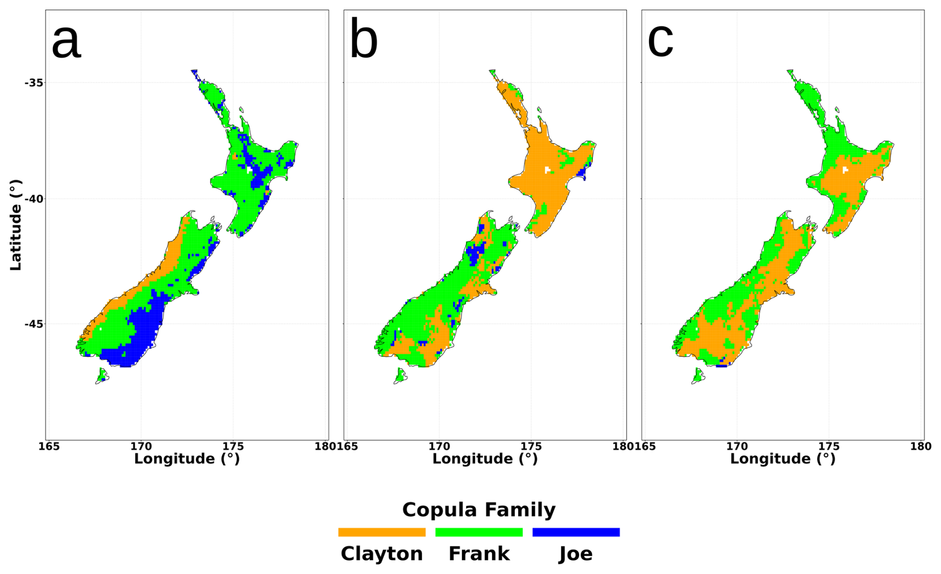
Figure 1 Spatial comparison of the optimal copula family for the pair copulas: Precipitation-Soil Moisture (a); Precipitation-Temperature (b) and Temperature-Soil Moisture, given Precipitation (c). Optimal family was determined using AIC for the period 1 January 1950 to 31 December 2021 and covering the entirety of New Zealand.

2.4 Construction of Copula Indices

2.4.1 Multivariate Vine Copula Index

After fitting a copula for each grid cell and calendar day, the resultant copula data (encompassing precipitation, maximum temperature and soil moisture; Table 1) were transformed into independent data in the [0, 1] space using a probability integral transformation (the Rosenblatt transformation, Rosenblatt, 1952). The Rosenblatt transforms $v:=(v_{\mathrm{1}},\mathrm{\dots },v_d)$ on the basis of the selected vine copula C for the data u= $(u_{\mathrm{1}},\mathrm{\dots },u_d)$ is defined as:

$$\begin{array}{}\text{(4)}& v_d:=C_{d\mathrm{|}\mathrm{1},\mathrm{\dots },d-\mathrm{1}}\left(u_d\mathrm{|}{u}_{\mathrm{1}},\mathrm{\dots },u_{d-\mathrm{1}}\right)\end{array}$$

where $C_{j|\mathrm{1},\mathrm{\dots }j-\mathrm{1}}$ is the conditional cumulative distribution function for variable j given the variables $\mathrm{1},\mathrm{\dots },j-\mathrm{1}$ for all $j=\mathrm{2},\mathrm{\dots },d$. In the Canonical Vine (C-Vine) context the order of the variables is determined by the selected order of root variables (Erhardt and Czado, 2018). Following the transformation into the [0, 1] space, the data is further transformed into a standard normal distribution using the inverse of the cumulative distribution function of a standard normal distribution:

$$\begin{array}{}\text{(5)}& p_j={\mathrm{\Phi }}^{-\mathrm{1}}\left(v_j\right)\end{array}$$

before being aggregated and standardised to the final Standardised Multivariate Index (SMI):

$$\begin{array}{}\text{(6)}& \mathrm{SMI}={\displaystyle \frac{\mathrm{1}}{\sqrt{d}}}\sum _{j=\mathrm{1}}^d{p}_j\end{array}$$

Limits of $-\mathrm{3}/\mathrm{3}$ were also imposed to ensure reasonableness with the extrapolation of return periods (Stagge et al., 2015). Each calendar day was then placed back into a sequential time series within each grid cell, resulting in the construction of the Standardised Multivariate Index (SMI). The SMI was then employed to characterise compound events. The 30 d accumulation was chosen due to the desired focus on monthly accumulations, with existing research on compound (Feng et al., 2021) and seesaw events (He and Sheffield, 2020) employing a similar one-month accumulation. Figure S7 illustrates a clustering performed on a 1 d accumulation of the SMI, highlighting known climatic regions of New Zealand when clustered outside temporal auto-correlation, while additional methodological detail is contained in Sects. S1 and S2 in the Supplement and Table S1.

Table 1 Climate indices constructed and used and their abbreviations.

2.4.2 Bivariate Copula Index

An additional bivariate copula index was also constructed, the Standardised Bivariate Index (SBI), following the same procedure listed above (with the exclusion of the vine copula components; Fig. 2). A bivariate copula index was constructed between soil moisture and precipitation (Table 1), to enable a comparison of these variables outside of the influence of temperature (i.e. the SBI is used to characterise seesaw event), with the bivariate copula construction between precipitation and soil moisture being a common copula pairing in multivariate hydroclimatic studies (AghaKouchak, 2015; Hao and AghaKouchak, 2013, 2014).

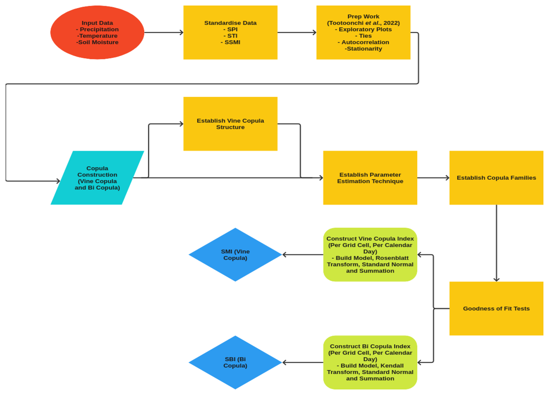
Figure 2 Flowchart illustrating the methodological procedure and steps performed in the current work to construct the multivariate index using both bi (Standardised Bi-Copula Index; SBI) and vine (Standardised Multivariate Index; SMI) copula methods.

2.5 Data Processing: Compound and Seesaw Events

Following the construction of the vine copula (SMI) and bivariate (SBI) indices, the relative performance of each approach was assessed against the more commonly employed coincident and consecutive approaches. Compound events were identified as the occurrence of low soil moisture (or precipitation) at the same time as that of high temperatures (De Luca and Donat, 2023). For the concurrent approach, a compound event day was identified if both STI and SSMI (SPI) were at or below −1, with dryness therefore defined by soil moisture (precipitation). For the vine copula, a compound event day was identified if the SMI and STI were both lower than −1 with dryness therefore defined by the joint probability between temperature, soil moisture and precipitation.

For seesaw events, the consecutive approach defines seesaw transitions as changes from dry to wet conditions (separately defined by single variable(s)) (He and Sheffield, 2020). Here, seesaw events were defined as the transition from −1 to +1 on the selected univariate (SPI or SSMI) indices. Bivariate transitions were identified as transitions from −1 to +1 on the SBI-30 index. Each index (SPI, SSMI and SBI) was first filtered to find both dry (−) and wet (+) phases that lasted longer than 30 d and that at least one day surpassed the threshold of −1 (dry) and +1 (wet) in standardised values. Seesaw events were defined as transitions from these dry to wet phases, utilising a 30 d buffer i.e. a wet phase must begin within 30 d of the dry phase ending.

2.5.1 Compound and Seesaw Event Frequency

To investigate the differences in event detection between the coincident (consecutive) and SMI (SBI) approaches, binary event occurrences were developed at each grid cell. These were then evaluated by comparing the event detection considering the SMI (SBI) approach as the true detection and developing a confusion matrix (e.g. error matrix). To illustrate, any day where both the SMI (SBI) and coincident (consecutive) approaches detect the same compound (seesaw) event is classed as a true positive, while any day where both approaches do not detect an event is classed as a true negative. If the SMI (SBI) approach detected a compound (seesaw) event day, which was not detected by the coincident (consecutive) approach, then this was classed as a false negative, while the detection of a compound (seesaw) event day under a coincident (consecutive) approach which is not present in the SMI (SBI) approach is classed as a false positive. The results at each grid cell were summarised by taking the mean across all days. For all compound event days at each grid cell, as defined by the SMI threshold, the mean of the STI and either the SPI or SSMI were extracted, as well as the STI value in isolation. These were then visualised as density plots of all grid cells. For seesaw events, density plots were constructed using the mean value for each grid cell as defined by the SBI approach i.e. the value of the SPI, SSMI and their mean for the same days that SBI identifies a seesaw event.

2.5.2 Run Theory

Run theory, commonly applied to drought analysis to calculate severity, intensity, duration and frequency (Panu and Sharma, 2002; Yevjevich, 1972), was used here to further investigate the differences in the representation of both compound and seesaw events under each classification. Frequency was defined as the total number of events. Duration is defined as the number of days below the exceedance thresholds (compound) or the average length of all seesaw events. Severity is defined as the cumulative sum of all index values. For compound events, the severity and intensity metrics for the coincident classification criteria were treated as the mean of SSMI/STI or SPI/STI. To minimise the effects of minor compound events, only those events which exceeded 14 d were investigated. Intensity is defined as the average of the index value for compound event days, while for seesaw events the intensity metric was replaced with a new metric: phase domination. Phase domination was defined as the combined total of both the lowest (dry) and highest (wet) value during the event, with negative values thereby indicating relatively stronger dry phases compared to the wet phase of the seesaw event (and vice versa).

2.5.3 Compound and Seesaw Event Characteristics

The onset rates (maximum compound event value over number of days to reach said value from the start of the event) and termination rates (maximum compound event value over number of days to cessation of event) were compared between each classification criteria for compound events, with the multivariate (SMI) approach used as the baseline i.e. SMI compared to coincident SSMI/STI, SMI compared to coincident SPI/STI (Fig. S2a–b). For seesaw events, the average transition time for each event was established for each grid cell, by taking the average number of days between the peak dry period and peak wet period, for all events at each grid cell, following the methods of Rashid and Wahl (2022). Differences between dry termination rates (minimum dry phase value over number of days to reach zero) and wet onset rates (maximum wet phase value over number of days to reach said value) were also calculated on a grid cell level (termed slope rates). Statistical significance was calculated using a t-test (Student, 1908), with 2000 iterations of a bootstrapping procedure performed (Wilkes, 2019), and adjusting p-values for spatial autocorrelation using the False Discovery Rate (FDR) approach (Wilkes, 2016). This method of comparison enables statistical confidence in the identification of events, but it should be noted that the suitability of the method at detecting historical events remains to be tested. In turn, this work will enable this future alignment by providing the necessary event identification dataset to ensure robust statistical testing.

3 Results

3.1 Compound Events

The coincident-approach low precipitation and high temperature metrics (SPI and STI) are in strongest agreement in the detection of compound event days with the SMI, with strong true positive (0.95) and true negative (0.95) values (Table 2). Conversely, coincident low soil moisture and high temperature (SSMI and STI) has lower agreement in compound day detection compared to the SMI approach, with true positive rates of 0.75 i.e. only 75 % of SMI defined compound event days are captured by the coincident approach of low soil moisture and high temperature. Despite this, true negative rates remain high (0.94).

Table 2 Confusion matrix for compound event detection. The matrix is created by treating the multivariate (SMI) detection as the true event occurrence.

A comparison of the relative severity of hot and dry compound events between the SMI and individual indices was achieved through analysis of SPI, STI and SSMI values on days when the SMI was below −1 (Fig. 3d). These results showed that the STI is typically more extreme than the SMI (STI mean of −1.76 vs. −1.58 for the SMI), while the SPI and SSMI are less extreme in the same situation (mean values of; SPI −1.11 and SSMI −1.02).

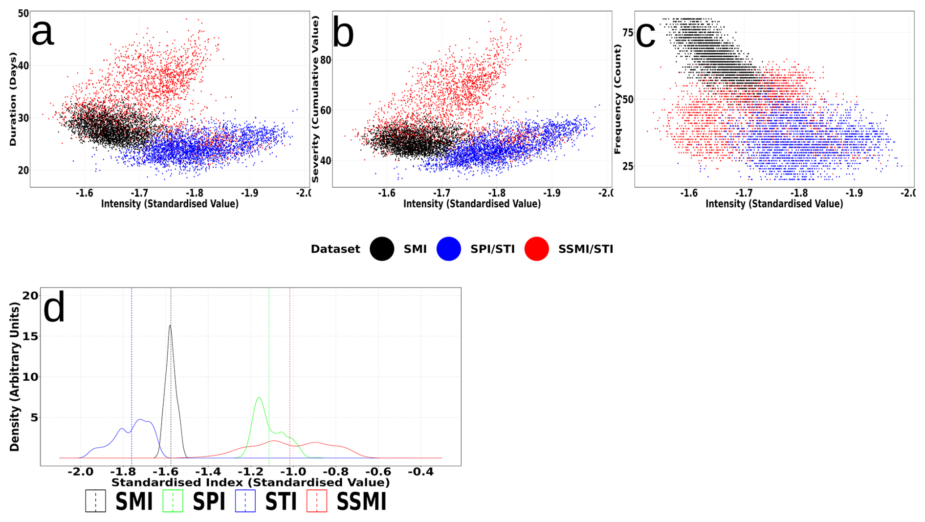
Figure 3 Duration (a), severity (b) and frequency (c) (y axis), mapped against intensity (common x axis), represented by the mean metric value at each grid cell. Note the different x and y scales within and between plots. Plots are for the multivariate (SMI) and coincident (SPI and STI; SSMI and STI) classification techniques. Also included are density plots (d), showing the distribution (SPI, SSMI and STI) during hot and dry conditions defined by the multivariate approach (SMI), with vertical dotted lines representing mean values.

SMI defined compound days are more frequent (median occurrence of 65 events) but less intense (median value of −1.62), while coincident SPI and STI and coincident SSMI and STI reveal less frequent (SPI/STI: 34, SSMI/STI: 47) and more intense (SPI/STI: −1.77, SSMI/STI: −1.67) events (Fig. 3a–c). This means that nationally there are 63 % more events when defined by SMI compared to coincident SPI/STI, and 32 % more events when defined by SMI compared to coincident SSMI/STI. Meanwhile, coincident SPI/STI compound events are characterised by short duration (24 d) and low severity (absolute value of 44), compared with SMI events (28 d and absolute severity of 47). In contrast, coincident SSMI/STI are characterised as long duration (32 d) and high severity (absolute value of 55) compared with SMI events. SMI defined compound days indicate much closer agreement countrywide, with less overall variation (and lowest values overall) in the relationship between intensity (value range of 0.23) and duration (day range of 11)/severity (absolute range of 19).

Spatial variation is the lowest for SMI defined compound days, with the least variation in intensity, duration and severity (Fig. 4c, f, i). Frequency (j–l) shows the most variation for run theory metrics (between 46 and 87 events), although compared to coincident metrics the variation is weaker (SPI and STI, frequency range between 15 and 58 events; SSMI and STI, frequency range between 14 and 66 events). Coincident SSMI and STI indicates the largest variation and highest values in all run theory metrics (a, b, d, e, g, h, j, k). Spatially, this large variation is expressed across the North Island (duration; 18 d and severity; absolute value of 39), with an extension into the west coast of the South Island for the intensity metric (variation in values of −0.28). The highest frequency of events (50 d) is visible across the upper east coast of the South Island and large parts of the North Island (52 d) under the coincident SSMI and STI approach, but remains less than the frequency expressed by the SMI approach (east coast of South Island: 72, North Island: 65).

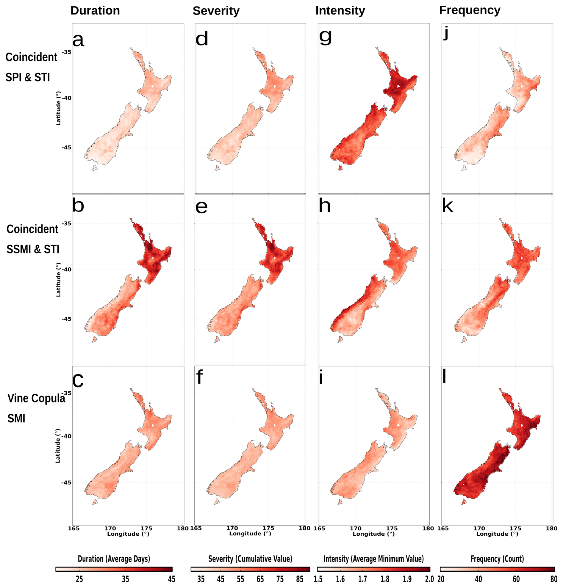
Figure 4 Average duration (a–c), severity (d–f), intensity (g–i) and frequency (j–l) of compound events on a grid cell basis for the period 1950–2021. Showing the coincident of −1 SPI and STI (a, d, g, j), coincident of −1 SSMI and STI (b, e, h, k) and co-occurrence of −1 SMI and STI (c, f, i, l). Note the differing scales.

All three approaches indicate longer duration (Fig. 4a–c) and stronger severity (d–f) of compound events in the mid and upper north of the North Island – albeit with less extreme values expressed in the SMI (duration; 8 d and severity; absolute value of 13) compared to coincident SSMI and STI. Intensity (g–i) is the most spatially variable of the metrics employed, with the most intense compound days across the upper and middle North Island and south of the South Island measured using coincident SPI and STI (mean minimum value of −1.8). This is captured to a lesser extent within coincident SSMI and STI (−1.7), and the SMI (−1.7). As a whole, intensity expressed by the SMI is the least variable amongst the three approaches, with the lowest intensity events across the east coast of both islands (mean value of −1.6). The mid and east coast of the North Island and mid to upper east coast of the South Island indicate the most frequent occurrence of events (j–l), with the SMI having 72 events compared to the coincident SPI/STI (42 events) and coincident SSMI/STI (51 events) approaches. For the wet west coast regions of New Zealand, more events are detected under the SMI approach (62 events) compared to coincident SPI/STI (33) and coincident SSMI/STI (44), however such events are of smaller intensity (SMI: −1.66; SPI/STI: −1.83; SSMI/STI: −1.77).

Compound event onset is more rapid for the multivariate SMI approach for much of the country. The largest differences in onset rates of compound events are revealed between those of the coincident SSMI and STI with the multivariate SMI approach (Fig. 5a–b). This consists of stronger onset rates (i.e. quicker onset, more severe or combination thereof) within the multivariate SMI approach against the coincident SSMI and STI approach. These differences are strongest across the west coast of the North Island (slope differences of −0.08), which is simultaneously the only region with weaker slope rates in the coincident SPI/STI approach compared to the SMI (slope differences of −0.02). Elsewhere, coincident SPI/STI reveals stronger onset rates, indicating a quicker onset/more severe (or combination thereof) compound events than the multivariate SMI approach (average slope difference of 0.03).

An overall general dominance of stronger coincident (SPI and STI) termination rates exists compared to that of the multivariate SMI termination rates (average slope differences of 0.12; Fig. 6a–b). This is strongest across the east coast of the South Island (slope differences of 0.15). The SMI also reveals stronger termination rates compared to the coincident SSMI and STI approach (average slope difference of −0.05).

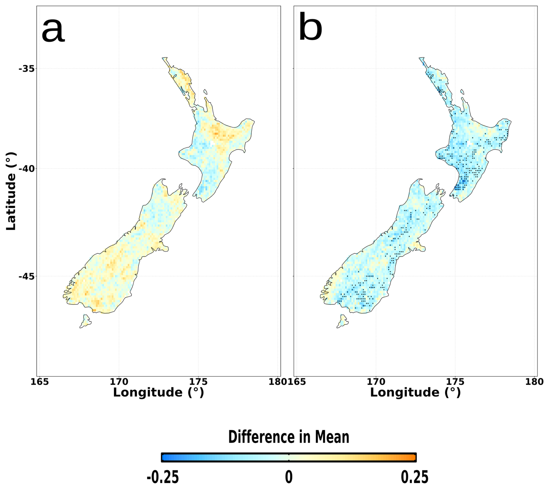
Figure 5 Differences in compound event onset slope rates between coincident (SPI and STI) and SMI (a), and coincident (SSMI and STI) and SMI (b). Average onset rates are calculated for each grid cell for the period 1 January 1950 to 31 December 2021. Note the differing scales. Stippling indicates significance at the 5 % level.

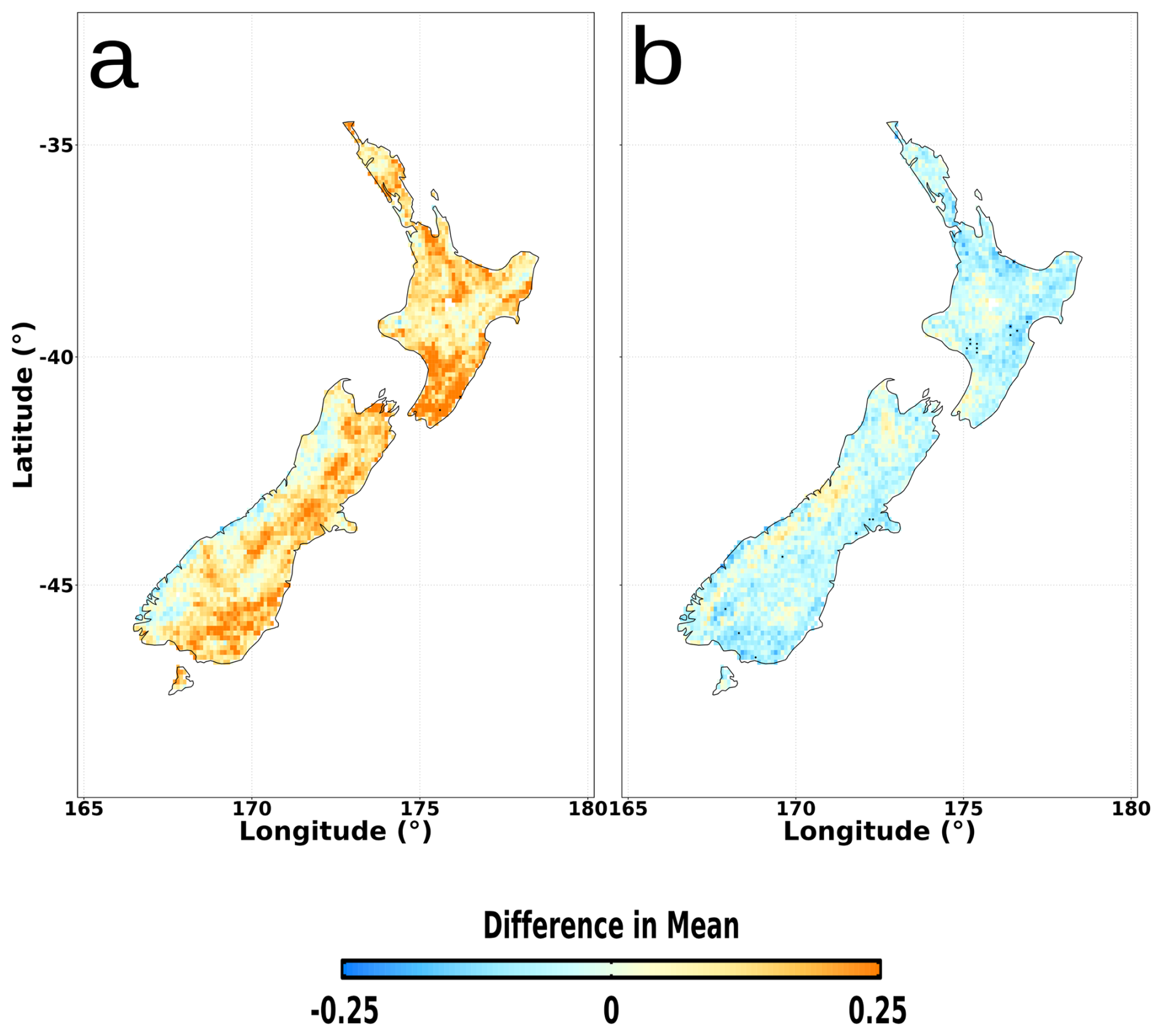
Figure 6 Differences in compound event termination slope rates between coincident (SPI and STI) and SMI (a), and coincident (SSMI and STI) and SMI (b). Average onset rates are calculated for each grid cell for the period 1 January 1950 to 31 December 2021. Note the differing scales. Stippling indicates significance at the 5 % level.

3.2 Seesaw Events

There is modest agreement in the detection of dry-to-wet seesaw event days between the SBI approach and the consecutive SSMI and SPI approaches (Table 3). Both true positive and true negative rates are similar between approaches, with agreement between SBI and SSMI of 0.56 and SBI and SPI of 0.59. True negative rates indicate greater agreement between SBI and SSMI (0.81) than the SBI and SPI (0.77), although the differences are minor.

SSMI values during SBI defined seesaw events are more strongly negative (i.e. less wet), with mean values of −0.18 compared to −0.02 in the SBI (Fig. 7d), and consecutive SPI (0.03). Little dominance in either phase is therefore present for SBI and SPI seesaw events.

Table 3 Confusion matrix for seesaw event detection. The matrix is created by treating the bivariate (SBI) detection as the true event occurrence.

Phase domination, duration and severity all indicate a similar distribution amongst the three classification approaches (Fig. 7a–c). Consecutive SPI seesaw events occur the most frequently (average of 79 d), while consecutive SSMI seesaw events show the most variation in event occurrence (variance of 99 events), with longer events generally characterised by a dry phase dominance (c). SBI seesaw events on the other hand reveal longer duration events (average duration of 149 d) as wet phase dominance increases, although an apparent tipping point is reached whereby this wet phase dominance becomes weaker (a).

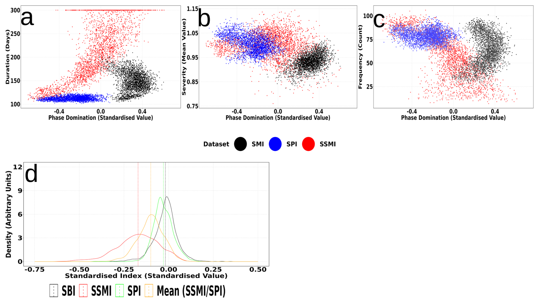
Figure 7 Duration (a), severity (b) and frequency (c) (y axis), mapped against phase domination (common x axis), represented by the mean metric value at each grid cell. Note the difference x and y scales within and between plots. Plots are for the bivariate (SBI) and consecutive (SPI; SSMI) classification techniques. Also included are density plots (), showing the distribution (SPI, SSMI and mean of both (SPI and SSMI)) during seesaw events defined by the bivariate approach (SBI), with vertical dotted lines representing mean values.

Consecutive SPI events are of the shortest duration (112 d), with the smallest range in duration (range of 23 d), while being of the strongest severity (absolute value of 1.0) (Fig. 7a–b). Consecutive SSMI events are of the longest duration (233 d), while SBI defined events have the largest range in duration (110 d) and are generally of lower severity (absolute value of 0.85) i.e. less extreme (a–b). SSMI events are of similar severity to consecutive SPI events (absolute value of 1.0), with the most severe events being wet side dominated (i.e. wet phase is longer; b–c). This wet phase dominance is most prevalent in SBI defined seesaw events, while for SSMI defined events longer duration, severe events tend to dominate across the wet phase (duration of 287 days for wet side dominated events against of 191 d for dry side dominated events; a–c).

Spatially, these differences in seesaw event run theory metrics are expressed as shorter duration events with lower severity across the west coast of the South Island for both the SSMI (duration of 135 d; severity of 1.00) and SBI (duration of 123 d; severity of 0.84) seesaw events (Fig. 8a–f). SSMI events are also dominated on the dry side across the west coast of the South Island (−0.38; h). SPI defined events meanwhile have an average duration of 115 days across the west coast of the South Island, which is characterised by a dry phase dominance (−0.19 average value; a, g). More generally, SBI seesaw events show a wet phase dominance across the entire country (absolute value of 0.31), compared to the dry phase dominance shown in the SSMI (−0.06) and SPI (−0.26) (g–i).

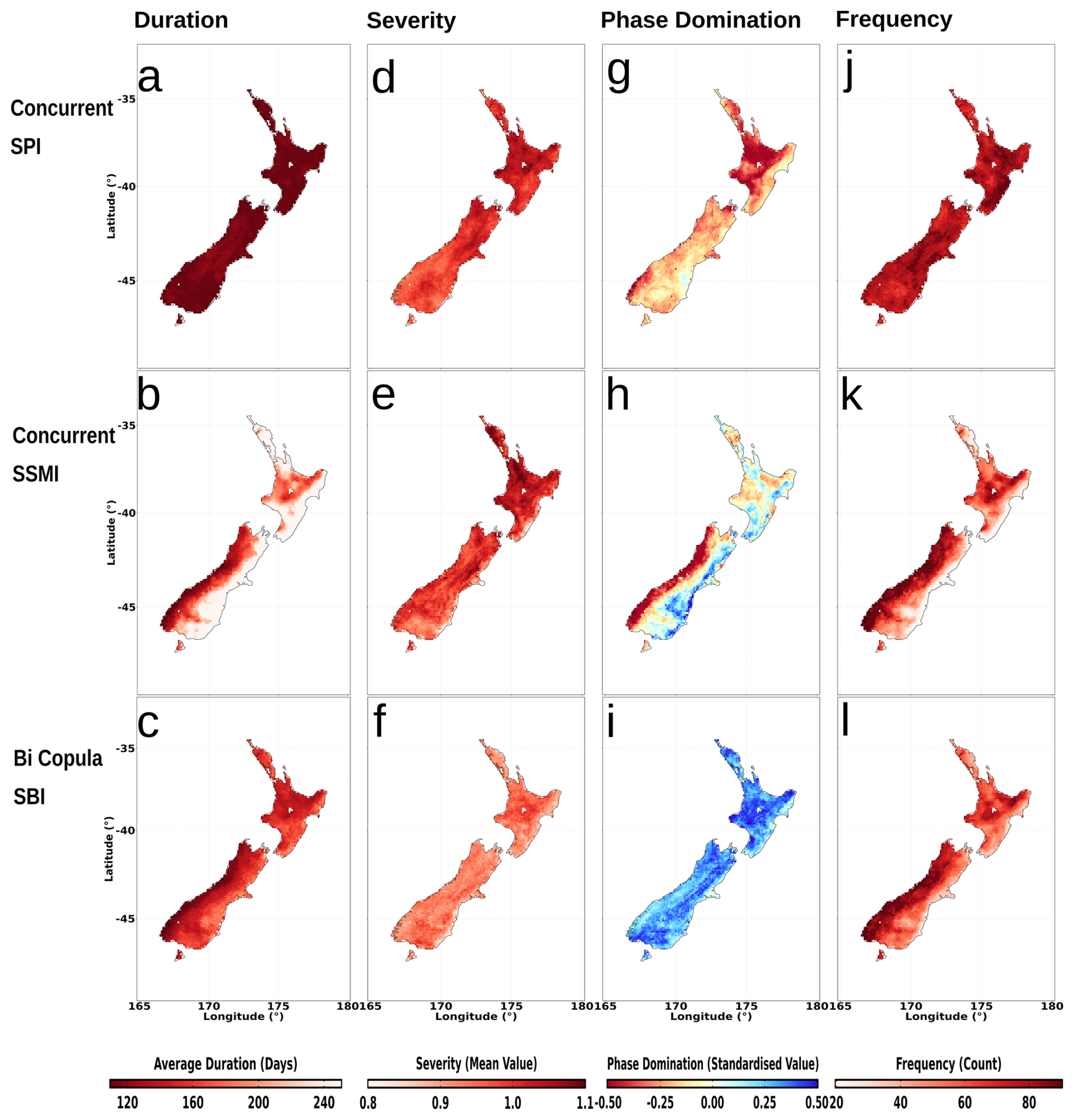
Figure 8 Average duration (a–c), severity (d–f), phase domination (g–i) and frequency (j–l) of seesaw events on a grid cell basis for the period 1950–2021. Showing the concurrent classifications of SPI (a, d, g, j) and SSMI (b, e, h, k), as well as the bivariate SBI (c, f, I, l). Note the differing scales.

SPI defined seesaw events occur the most frequently, which is strongest across the west coast of both islands with 80 events under the SPI approach compared to the SSMI (62 events) and SBI (64 events) (Fig. 8j–l). Agreement for the frequency of events across the three metrics is strongest between SBI (62 events) and SSMI (57 events) classifications, with an overall higher occurrence of events under the SPI (79 events) classification. While the west coast of the South Island remains a high frequency region under the SPI approach (79 events), more events are detected with the SBI (84 events) and consecutive SSMI (85 events) approaches. Finally, east coast of both islands display the greatest variation in event occurrence, with a total difference of 40 events (SBI: 42 events; SSMI: 53 events; SPI: 82 events).

Seesaw transitions (time from −1 to +1) show an overall longer transition time for SSMI based classifications compared to SPI and SBI based classifications (Fig. 9b; transition time of 107 d). The longest transition times are present on the east coast of both islands for SSMI based classification (132 d), and SBI based classification (88 d), while the SPI classification reveals the shortest transition time across the three classification criteria (56 d; a–c). The west coast of the South Island reveals the shortest transition times, with transition times of SSMI (65 d), SPI (60 d) and SBI (68 d) (a–c).

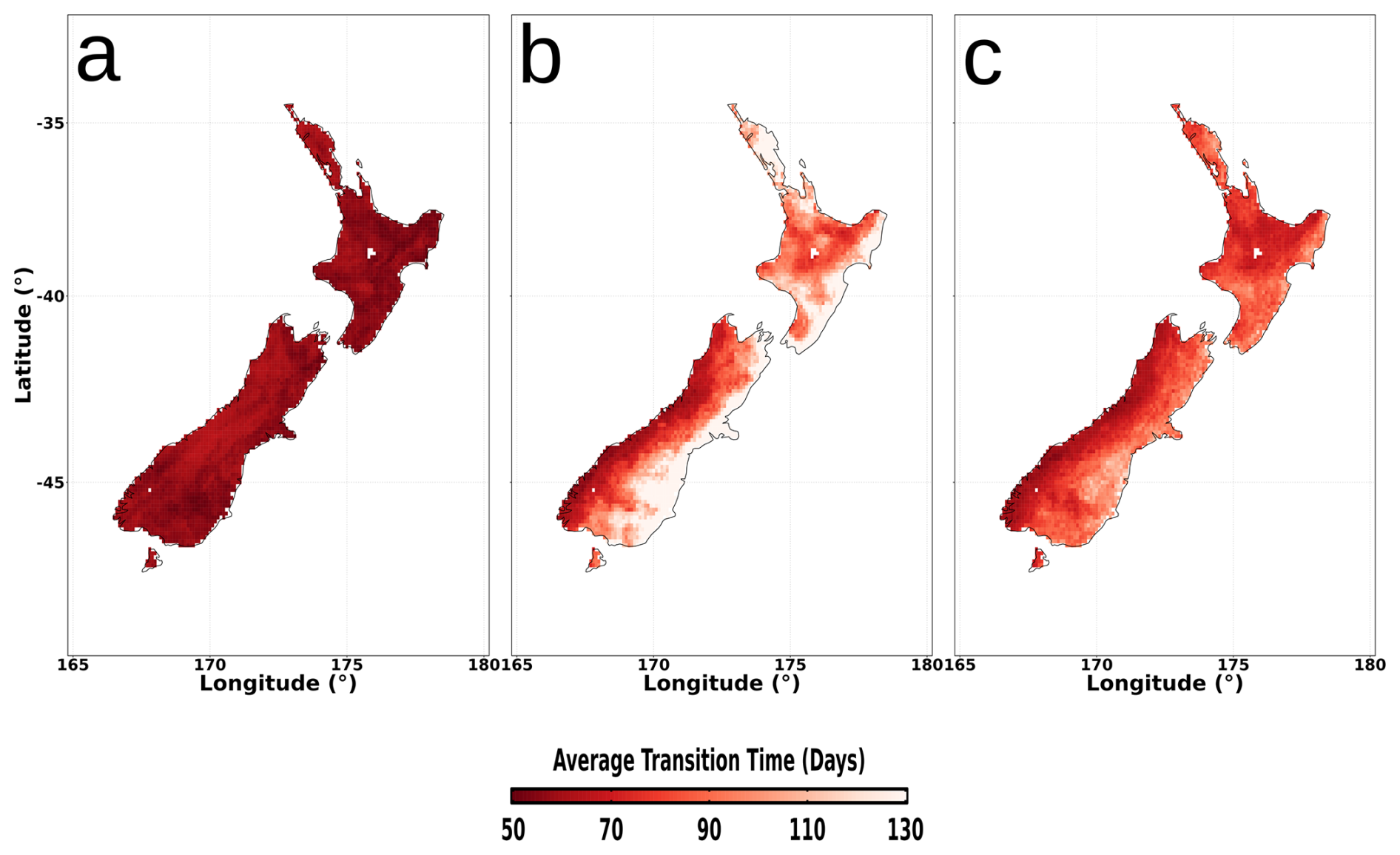
Figure 9 Average transition time (days) of seesaw events for SPI (a), SSMI (b) and SBI (c) classifications. Transition time is defined as the amount of time taken to pass from the peak dry value to the peak wet value.

Nationally, SPI defined events have the strongest dry terminations rates (statistically significant; slope difference of 0.04), while stronger wet onset rates are present for SSMI (average slope difference of −0.01) and SBI defined events (average slope difference of −0.02) (Fig. 10a–c). The east and west coasts of the South Island reveal contrasting termination/onset rates to that expressed by individual metrics. On the east coast, SPI defined events have stronger wet onset rates (minimum slope difference of −0.05), while SBI defined events have stronger dry termination rates (maximum statistically significant average slope difference of 0.04) (a–b). For the west coast of the South Island a similar contrast emerges, with stronger dry termination rates under the SSMI approach (significant slope differences of 0.01) compared to the stronger wet onset rates under the SBI approach (significant slope differences of −0.02) (b–c).

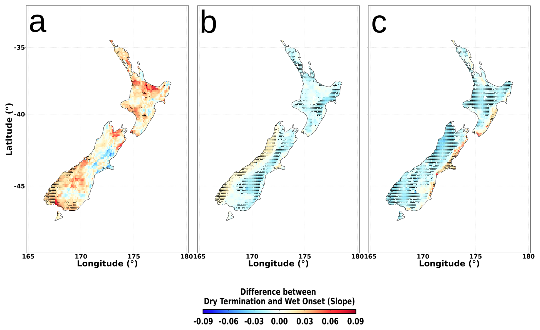
Figure 10 Differences in slope rates between dry termination and wet onset rates of seesaw events for the period 1 January 1950 to 31 December 2021 for SPI (a), SSMI (b) and SBI (c) classifications. Stippling indicates significance at the 5 % level.

Differences in event characteristics are strongest across the east coast of the North Island (transitional regime), with long duration, high severity and low frequency events represented by the SSMI and SBI, compared with the SPI representation as short duration, low severity and high frequency events. Notable slope rate differences between drought termination and wet onset are also present (Fig. 10a–c). The slower responding soil moisture indicates much of east coast as having a significantly quicker onset of wet phases (relative to drought cessation) (Fig. 10b). Consecutive SPI also reveals parts of the east coast as having quicker wet onset phases, although such differences are not significant. Contrasting this, the copula approach reveals weaker wet phase dominance across the east coast of both islands (Fig. 10c).

4 Discussion

4.1 Compound Events

4.1.1 Examination of Regional Variation in Compound Events

For the east coast of both islands (examples of transitional regimes, being regions where soil moisture constrains evapotranspiration variability, Seneviratne et al., 2010), SPI/STI events have the strongest agreement in severity and duration to the SMI (Figs. 3a–b, 4a,d). This is in contrast to the longer duration and stronger severity observed within the coincident SSMI/STI detection method, which also drives their faster onset and termination rates (Figs. 3a–b, 4 b, e, 5a–b, 6a–b). Thus, a more common (and more extreme) temperature anomaly is visible within coincident soil moisture/high temperature, resulting in longer duration (and subsequently stronger severity) events, reflective of the underlying surface energy balance exchanges (e.g. increased sensible heat) taking place during compound event occurrence (Seneviratne et al., 2010).

The strong relationship between low soil moisture and high temperature (given precipitation – i.e. lower tail dependence) in the vine copula results in a more common occurrence of compound events within the SMI than coincident approaches (i.e. not accounting for the dependence between soil moisture and temperature). A higher frequency of events across the east coast of both islands is also shown in Bennet et al. (2023), demonstrating the importance of compound events for these regions of the country, and in agreement with the findings that extreme temperatures impact these regions (Harrington, 2021; Harrington and Frame, 2022). This is expressed across the east coast regions as high event occurrence across all metrics (SMI: 72 events; SSMI/STI: 51 events; SPI/STI: 42 events). Put another way, a 1 in 100 year event defined by the SMI across these east coast regions becomes a 1 in 171 (SPI/STI) or 1 in 141 (SSMI/STI) year event. Such variation has vital implications for hazard management and planning, and illustrates the importance of understanding uncertainty in compound hot and dry event detection which is driven by the choice of dry indicator (Hosseinzadehtalaei et al., 2024).

The identification of agricultural dry conditions in wet, energy limited regimes (i.e. displaying lower tail dependence; Cammalleri et al., 2024) is impacted by the vine copula approach to a greater extent than transitional regimes. The representation of agricultural drought via the SMI captures a higher occurrence of dry phases, with the lower tail dependence resulting in the largest difference in event frequency compared to the coincident approaches (Fig. 3a–c). Similar to transitional regimes, precipitation metrics for agricultural drought identify the least number of compound events, reflecting the delay in moisture deficit propagation into soil moisture (Zhu et al., 2021). The lower number of agricultural droughts identified using precipitation metrics is further supported by Bachmair et al. (2018) who identified that meteorological indices (e.g. SPI) were less informative of agricultural drought across colder/wetter regions in Europe.

Building on the findings of Bachmair et al. (2018) that precipitation metrics are less informative of agricultural drought in wet regions, the present research generates the greatest disparity between detection methods across wet regions. For example, the west coast of both islands indicate large variation in events across all three metrics (SMI: 62; SSMI/STI: 44: SPI/STI: 33), which simultaneously indicate a weaker intensity (SMI: average intensity of −1.66; SSMI/STI: average intensity of −1.77: SPI/STI: average intensity of −1.83) i.e. more frequent, less intense under the SMI approach. For the west coast of the South Island, the high occurrence of events captured by the SMI results in events which are shorter, less severe and less intense than the coincident SSMI/STI approach or the high intensity coincident SPI/STI approach. For example, low severity events (defined as the 25th percentile of SMI events) with a 1 in 100 year return period equate to a 1 in 181 (SSMI/STI) or 1 in 219 (SPI/STI) year event. Meanwhile, high severity events (75th percentile of SMI) with a 1 in 100 year event (SMI) equate to a 1 in 160 (SSMI/STI) or a 1 in 210 (SPI/STI) year event. While dry indicator uncertainty for compound hot and dry events is significant in general (Hosseinzadehtalaei et al., 2024), the regional variation shown here indicates that the greatest sensitivity to dry indicator selection is found across wet energy limited regions.

4.1.2 SMI Detection of Compound Events

The spatial expression in event occurrence for New Zealand shown here (0.64 to 1.21 events per year based on the SMI) was also shown in Bennet et al. (2023), where a range of 0.21 to 1.14 events per year was identified using coincident SSMI/STI. The coincident metrics currently employed, being SPI/STI (0.19 to 0.92 events per year) and SSMI/STI (0.21 to 0.81 events per year), both reveal an overall lower frequency compared to that reported in Bennet et al. (2023). An overall higher frequency of events is present across the entire country for the SMI (median of 65 events) compared to the coincident approaches (SSMI and STI (47 events); SPI and STI (34 events)) (Figs. 3c, 4j–l). This is expressed as a 63 % difference under the SMI compared to the coincident SPI/STI approach, and a 32 % difference compared to the coincident SSMI/STI approach. Such differences suggest careful consideration should be made to the choice of dry indicator for any study involving compound hot and dry events (e.g. establishing trends or projected changes) (Hosseinzadehtalaei et al., 2024).

Nationally, the soil moisture/high temperature anomaly is more common than precipitation/high temperature (Fig. 3d), indicating the difficulty of detecting co-occurring low precipitation and high temperature anomalies with the coincident approach (Tabari and Willems, 2023; Zscheischler and Seneviratne, 2017). The use of precipitation as a proxy for agricultural drought (coincident SPI/STI) identifies the least number of compound events, an outcome of the delay in moisture deficit propagation from atmosphere to soil moisture (He and Sheffield, 2020). The usage of any precipitation metric as a proxy for soil moisture and agricultural dry conditions should only be made after careful consideration of the appropriate accumulation period, necessitating a regional specific prior analysis and acknowledgement of possible spatial variation in appropriate accumulation periods (Wang et al., 2022). Without this prior analysis, soil moisture-based approaches should be the default for investigating compound hot and dry events.

Meanwhile, representing agricultural drought as the dependence between soil moisture and precipitation (Hao and AghaKouchak, 2013) results in the highest detection of compound events (SMI) nationally. The use of the vine copula approach for agricultural drought representation in compound event detection enables a greater understanding of the impact regional differences in variable anomalies have on compounding conditions (e.g. stronger termination rates for lower tail dependency regions (east coast of New Zealand) or more frequent events in wet, energy limited regions). The vine copula approach simultaneously reveals a greater frequency of this agricultural dry phase than solely precipitation or soil moisture (Hao and AghaKouchak, 2013). Thus, while uni variate soil moisture-based approaches are still recommended for investigating compound hot and dry events, multivariate approaches (SMI) identify events which would go undetected when solely using soil moisture. Multivariate approaches may therefore provide a more accurate description for both risk and hazard management as well aid in accurate identification of wider atmospheric controls and teleconnections. This accurate description and identification by multivariate approaches is achieved by revealing the true probability for hot and dry co-occurrence and therefore should be utilised whenever possible

4.2 Seesaw Events

4.2.1 Examination of Regional Variation in Seesaw Events

Similarities are strongest between approaches across wet, energy limited regions. The west coast of the North Island shows a similar pattern of high frequency occurrence (SBI: 64 events; SSMI: 62 events; SPI: 80 events) and phase domination (SBI: mean value of 0.33; SSMI: mean value of −0.20; SPI: mean value of −0.33). Meanwhile, the average transition time is lowest across the west coast of the South Island under all measurement techniques (Fig. 9a–c). Differences are most noteworthy between approaches in the representation of slope rate differences between drought termination and wet onset (Fig. 10a–c). Consecutive SPI reveals significant parts of the country (upper-mid North Island, north and south of South Island) as having rapid drought cessation relative to wet onset (Fig. 10a), driven by the return to relatively wet conditions in these wet regimes (Bennet et al., 2023). For the west coast of the South Island, the SSMI representation of seesaw events reveals a stronger dry termination rate, evidence of the comparatively wet environment witnessing a return to the wet, normal conditions. Contrasting this, the copula approach reveals much of the country has quicker wet phase onsets – it is noted that this is the generally expected response given the required time to recover from dry or drought conditions (Rashid and Wahl, 2022).

The emergence of stronger wet phases in the SBI across wet energy-limited regions becomes apparent due to the lower tail dominance (Fig. 1), whereby agricultural drought detection is greater (Cammalleri et al., 2024) in the west coast (Fig. 8l) (an outcome of the more common agricultural drought phase driven by the slow responding soil moisture i.e. weaker but more frequent agricultural drought). In turn, this more common drought phase and lower tail dominance drives weaker termination rates relative to the onset rate of the wet phase in the SBI (slope difference of −0.02). Contrasting this, consecutive metrics reveal stronger dry termination rates (Fig. 10c), a result of the stronger dry phases relative to wet phase (i.e. stronger, less frequent agricultural drought; Fig. 8g–i).

The west coast of the South Island is characterised by its exposure to the westerly passage of air movement which drives New Zealand weather systems (Macara, 2018), as well as large atmospheric river events which bring substantial precipitation (Prince et al., 2021). Therefore, the high occurrence of seesaw events (Fig. 8c) is somewhat expected. Further, De Luca et al. (2020) note a domination of wet over dry extremes in wet climates across the globe. Combined with a greater identification of agricultural drought across these wet regions (i.e. lower tail dependence; Cammalleri et al., 2024) (Fig. 1), a relatively high number of both dry and wet events results, with a subsequent increased likelihood of these occurring consecutively. However, of note is the severity of such events being comparatively minor, likely driven by their short duration (Fig. 8a–c).

The consistent finding that seesaw events on the South Island west coast are typically high frequency, short duration and low severity for each of the SBI, SSMI and SPI (Figs. 6, 7, 8) is consistent with the findings for this region in the global-scale study of Rashid and Wahl (2022). Similarly, return periods are similar between the three indices – overall, indicating little difference in detection metrics across wet energy-limited regions such as this, and in stark contrast to these regions having the strongest differences between metrics for compound hot and dry events (Figs. 3, 4, 7, 8).

The strong differences in seesaw event characteristics across the transitional regime of the North Island east coast (long duration/high severity/low frequency for SSMI and SBI, vs. opposing characteristics for the SPI) are associated with notable slope rate differences between drought termination and wet onset (Fig. 9). The slower responding soil moisture indicates much of east coast as having a significantly quicker onset of wet phases (relative to drought cessation) (Fig. 10b). Consecutive SPI also reveals parts of the east coast as having quicker wet onset phases, although such differences are not significant. Contrasting this, the copula approach reveals weaker wet phase dominance across the east coast of both islands (Fig. 10c).

The weaker wet phase dominance in the SBI approach is present due to the upper tail dominance (Fig. 1) resulting in a more frequent wet or pluvial phase under the joint probability framework (Fig. 8). With evapotranspiration (including seasonal variation) becoming a controlling factor in moisture loss in transitional regimes (Seneviratne et al., 2010), no distinguishable lower tail relationship is present across these east coast regions under the SBI approach (Fig. 1), resulting in more rapid shifts out of the dry phase into the more common wet phase (e.g. the upper tail dependence) (Fig. 10c).

East coast regions reveal the largest variation between event detection (SBI: 53 events; SSMI: 42 events: SPI: 82 events), as well as the longest transition time in the SBI (88 d) and SSMI (132 d) driven by the slow responding soil moisture and upper tail dominance in the SBI. The high occurrence across east coast regions described by the SPI is similarly reflected in Bennet et al. (2023), where up to 18 % of droughts were terminated by a pluvial. Translated into return periods, a 1 in 100 year event as defined by the SBI results in a 1 in 126 (SSMI) and 1 in 65 (SPI) year return periods. Dry indicator selection therefore has the most uncertainty across the east coast of both islands (transitional regimes), with key implications for water management practices illustrated in the range in return periods.

4.2.2 SBI Detection of Seesaw Events

Collectively, the SBI representation of seesaw events exists in the middle between the SSMI (57 events) and SPI (79 events) detection approaches, with a spatial average of 62 events across the country. As a spatial average, SBI events are dominated on the wet side (mean value of 0.31), characterising SBI-defined transitions as having longer or more intense wet phases during seesaw events in comparison to the dry phase dominance shown in SPI (mean value of −0.26) and SSMI (mean value of −0.06) (e.g. more intense or longer dry phases). Nationally this is expressed as a range in return periods of 30 years using SBI as the 1 in 100 year baseline (SPI: 1 in 79 years, SSMI: 1 in 109 years).

Wet, energy limited regions show the greatest agreement between approaches, with precipitation and soil moisture seesaw progressing at a comparatively similar speed. In contrast, seesaw events across transitional areas have the largest deviation between precipitation and soil moisture seesaw, indicative of evapotranspiration becoming a controlling factor (including seasonal variation) in dry phase development during soil moisture seesaw. Consistent with the existing research on drought quantification uncertainty (Mishra and Singh, 2010) (Stagge et al., 2017) (Vicente-Serrano et al., 2012), the present work illustrates variation in seesaw event detection and characteristics dependent on the chosen representative variable (Figs. 7a–c; 9a–c, 10a–c).

Similar to compound hot and dry events (e.g. Hosseinzadehtalaei et al., 2024), sensitivity to selection of dry indicator for seesaw events is expected. However, unlike the recommended use of soil moisture metrics for compound hot and dry detection (and preference for multivariate representation of agricultural drought), no one method should be ultimately termed “superior” for seesaw detection, reflecting the more general comments by Lloyd-Hughes (2014) on drought detection. Accordingly, care is needed to fully differentiate studies according to the hydrological domain(s) implied by the dry phase/drought type targeted and subsequent index selection (Hoffmann et al., 2020) (e.g. precipitation seesaw, soil moisture seesaw). The differences in frequency and return periods of water deficits in different hydrological cycle domains can have vital implications for water management practices as well as the understanding of driving mechanisms and wider teleconnections. For New Zealand, east coast regions show the largest difference in detected events, and with these regions being key agricultural centres and sources of significant hydropower generation, not framing the study around the desired hydrological cycle component could have significant implications.

5 Summary and conclusions

While a need to investigate the interconnectedness of hydroclimatic variables is necessary for extreme compound events, the complexity in drought quantification itself must not be overlooked. Relating to the first objective of this study (to determine the difference in occurrence and characteristics of extreme hydrometeorological compound and seesaw events in New Zealand using copula-based and convectional methods), the more variable precipitation metric coincides less frequently with high temperatures (median event occurrence of 34 events) in comparison to soil moisture (47 events). Multivariate representation of agricultural drought however identifies a greater occurrence of high temperature and dry conditions, with 65 events across the country. This higher frequency of events is contrasted with the comparatively lower intensity of events, with median intensity in the SMI of −1.62, compared to SSMI/STI of −1.67 and SPI/STI of −1.77. Relating to the second objective of the study (highlight the regional variation in compound and seesaw event quantification), regional differences in compound event characteristics are evident, with the wet, west coast regions of the country showing a stronger pattern compared to the nationwide metrics. This is manifested as more detected events using the SMI approach (62 events) compared to the coincident approaches (33 SPI/STI and 44 SSMI/STI), but with a correspondingly weaker intensity in compound events e.g. more common and less extreme (average intensity in SMI of −1.66, SSMI/STI −1.77, SPI/STI −1.83). Across the west coast of the South Island, this equates to low severity events having return periods of 1 in 181 (SSMI/STI) or 1 in 219 (SPI/STI) compared to the baseline 1 in 100 year SMI event.

Seesaw event detection using a bivariate copula methodology identifies many instances of seesaw behaviour across the country. Average differences between the SBI representation of seesaw events (spatial average of 62 events), the SSMI (spatial average of 57 events) and the SPI (spatial average of 79 events) results in vital differences in return periods, with a 1 in 100 year event under the SPI approach becoming a 1 in 128 year (SBI) or a 1 in 139 year (SSMI) event. Across wet, energy limited regions (e.g. the west coast of the North Island), agreement is strongest in the identification of seesaw events, with 64 events detected under the SMI, 62 events detected using the SSMI and 80 events using the SPI. This agreement is driven by the compatibility in identifying dry phases in wet regions across all metrics, with stronger wet onset rates in the SBI (slope difference of −0.02) an outcome of the more common agricultural dry phase representation and identification of high frequency events. Contrasting this, differences are greatest across the east coast regions of the country (transitional regimes), where evapotranspiration plays a greater role in dry phase development, resulting in the longest transition time (average of 92 days across all metrics) and largest variation in detection methods (42 events detected using the SSMI, 53 using the SMI, and 82 using SPI).

Addressing the third objective of this study (provide recommendations as to the usage of detection methods for compound and seesaw events), the inclusion of more variables as a representation of drought results in more variation in the resultant index, representing the hydrological cycle to greater extent (e.g. SMI vs SBI). Employing the often-used drought definitions (e.g. Mishra and Singh, 2010), the dry component of compound hot and dry events is arguably representative of an agricultural drought. For compound event detection then, soil moisture-based metrics are recommended, ideally as a multivariate representation of agricultural drought, with precipitation-based metrics only suitable if significant prior work is performed to understanding how precipitation deficits propagation into soil moisture. For seesaw event detection, a need is shown to frame rapid transitions in hydrological states within the framework of the hydrological cycle more commonly employed within drought research: as rapid meteorological or agricultural transitions. In turn, multivariate representation via bivariate means provide an intermediary method that highlights the regional variation in the propagation of meteorological to agricultural drought and the resultant impact this has on rapid transitions.

Both compound and seesaw events are complex hydrometeorological events, the study of which is made further complex due to the inherent uncertainty in drought quantification. The use of multiple variables to define the drought phase enables the characteristics unique to different physical forms of drought to be captured. The multivariate framework provides not only a means to encapsulate these multiple variables, but to do so in a manner that respects the regional variation in the dependence structure between them. With significant work now present in the detection of compounding and seesaw event behaviour across New Zealand, research should now be directed towards understanding the driving mechanisms responsible for these events i.e. wider atmospheric controls. Continuing to understand the differences in compound event detection under differing drought classifications, particularly under projections of a changing climate, should also remain a top priority. For water management, unravelling the regional variation and mechanisms responsible for the differing pace of seesaw transitions also remains a key research objective.