Filling data gaps in soil moisture monitoring networks via integrating spatio-temporal contextual information

As critical inputs for global climate studies, watershed hydrologic modeling, and satellite soil moisture product validation, in situ soil moisture measurements are frequently compromised by sensor-derived data gaps that disrupt hydrological continuity. To overcome this challenge, we develop ST-GapFill, a novel spatiotemporal reconstruction framework integrating multi-source contextual information through two key innovations: (1) Spatial correlation-guided neighbor selection that identifies optimal auxiliary stations; (2) a long short-term memory (LSTM) network is employed to capture the complex temporal dependencies within the soil moisture time series. Validation on in-situ networks demonstrates that ST-GapFill successfully reconstructs soil moisture dynamics with preserved diurnal-phase fluctuations, achieving 0.91 correlation coefficients with ground truth under low missing-rate conditions (< 50 %). Comparative analysis reveals the ST-GapFill's statistically superior performance (RMSE reduction: 27.0 % vs. IDW, 67.8 % vs. ARIMA). This method establishes a robust spatiotemporal imputation paradigm for environmental sensor networks, effectively bridging observation gaps to support precision agriculture and climate change impact assessments.

1 Introduction

Soil moisture (SM) plays a critical role as a key factor in land-atmosphere interactions, significantly influencing crop growth and surface evapotranspiration capacity. It is not only an important component of the global water cycle and water balance, but also an important indicator of global climate change (Galvincio et al., 2024). SM monitoring plays an important role in agriculture, ecology, and water resource management (Zhou et al., 2021; Humphrey et al., 2021). Stable and continuously consistent long time series SM data are critical for global environmental and climate change monitoring. Wireless sensor networks (WSN) have become an important means of acquiring SM for the advantages of small size, low cost, and easy deployment (Dorigo et al., 2021). However, missing data is common in soil moisture wireless sensor network systems. Factors such as power outages, emergency maintenance, and communication failures can lead to data loss from some or all sensors. These data gaps not only affect the effectiveness of real-time monitoring, but also negatively impact subsequent applications such as trend analysis and time-series prediction. Therefore, accurately filling missing values at specific sites and constructing continuous time-series data has become a key challenge in practical applications (Sadhu et al., 2020; ur Rehman et al., 2018).

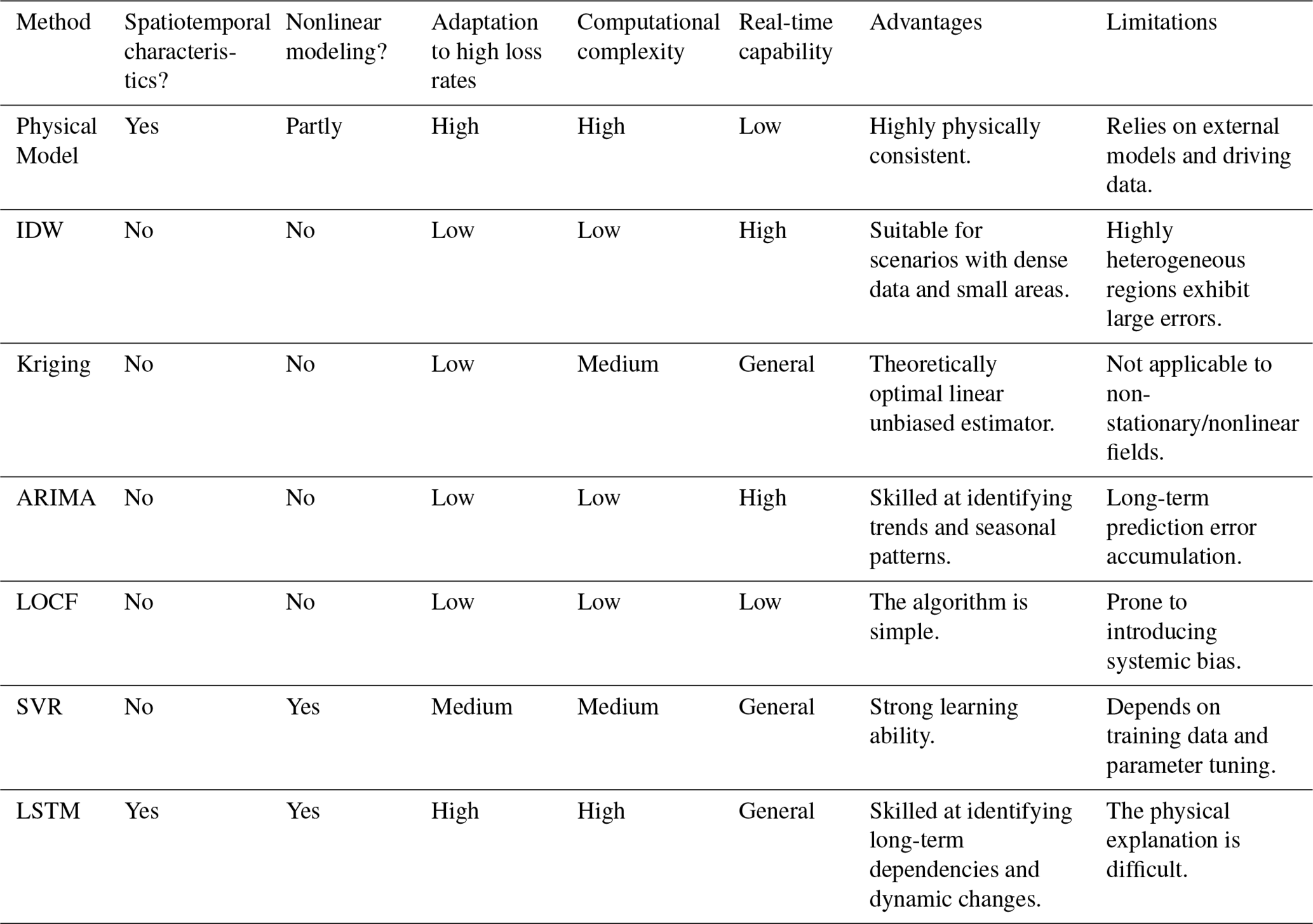
Currently, methods for filling gaps in spatiotemporal SM data can be categorized based on criteria such as whether they employ physical models, account for nonlinearity, and consider spatiotemporal coupling characteristics. These include: methods based on physical process models, traditional statistical/deterministic interpolation methods, machine learning methods, and deep learning methods. A performance comparison table for different methods is shown in Table 1. Physics-based methods (such as land surface hydrological modeling or data assimilation) generate spatiotemporally continuous and physically consistent SM data by incorporating constraints from physical processes like precipitation-runoff relationships (Wei et al., 2024). Their interpolation results align with objective mechanisms but rely on model-driven data and remain sensitive to model biases. Traditional statistical and deterministic interpolation methods rely on predetermined mathematical model assumptions (e.g., spatio-temporal smoothness and continuity of SM) to extrapolate data using historical observations from the same location or nearby sites. For example, time series interpolation commonly employs models such as linear interpolation (Kreindler and Lumsden, 2016), Last Observation Carried Forward (LOCF) (Lachin, 2016) and autoregressive integrated moving average model (ARIMA) (Shumway and Stoffer, 2017). The advantages include model simplicity and computational efficiency, providing reliable estimates when the missing rate is low and the variation is stable. For instance, Yamark and Gadosey (2019) compared the application of ARIMA and deep learning models in climate data time series interpolation. In scenarios with a missing rate < 10 % and stable seasonal trends, the ARIMA model outperformed LSTM/GRU models. However, the drawbacks include an inability to reflect spatial heterogeneity and difficulty in handling strongly nonlinear fluctuations. Spatial interpolation methods such as inverse distance weighting (Dhevi, 2014) and Kriging (Oliver and Webster, 1990) utilize spatial autocorrelation to fill missing values. Their advantages lie in intuitive algorithms and low requirements for sampling patterns. Limitations include consideration only of spatial neighborhoods, neglect of temporal trends, and typical assumptions of linear relationships, which fail to capture complex nonlinear processes (Wang et al., 2024). Kuo et al. (2021) used a kriging estimator to obtain local weather data. The accuracy of the weather station estimator is slightly lower than that of the local sensor estimator. Xie et al. (2020) used four methods – IDW, ordinary kriging, multiple linear regression with residual kriging, and radial basis function neural network with residual kriging – to interpolate large-scale SM in deep soil layers. However, the randomness and complexity of SM missing values limit the universality of these methods. In contrast, machine learning methods (such as support vector machines and random forests) and deep learning approaches (e.g., long short-term memory networks, LSTM) can learn nonlinear spatiotemporal relationships from data, demonstrating stronger capabilities in characterizing the multifactorial influences on SM. These data-driven approaches can incorporate multi-source information, such as observations from neighboring sites and meteorological elements, into their models. Consequently, they exhibit higher reconstruction accuracy under scenarios with extensive spatial coverage and high data missing rates (Chhabra et al., 2018). Deep learning models, in particular, can simultaneously capture both the spatial patterns and temporal dynamics of data, proving superior to traditional interpolation methods in reconstructing long-term missing values. Mao et al. (2019) proposed a deep neural network multi-view learning approach to reconstruct spatio-temporal data from five perspectives: global spatial, global temporal, local spatial, local temporal, and semantic, to fill in successive missing readings of the sensor. Rivera-Muñoz et al. (2022) proposed a novel matrix factorization technique (i.e., deep matrix factorization or DMF) via a neural network architecture for estimating missing data in WSNs. Yi et al. (2016) proposed a spatio-temporal multi-view learning-based approach that considers both the temporal correlation between different time-stamped readings in the same time series and the spatial correlation between time series at different locations. This method enables the filling of gaps in geo-aware time-series data sets. It should be noted that while machine learning and deep learning models offer high accuracy and broad applicability, they exhibit strong dependence on training data volume, feature complex model structures, and lack physical interpretability (Wang et al., 2024). Therefore, in studies addressing missing SM data, appropriate methods should be selected based on application requirements: physically constrained models are preferable when emphasizing physical reliability; traditional statistical methods suffice for linearly stationary data with few missing values; whereas spatio-temporal modeling methods integrating machine learning/deep learning are undoubtedly the optimal choice when dealing with complex spatiotemporal dynamics and significant nonlinearity (Zhao et al., 2022; Shangguan et al., 2023).

Table 1 Performance Comparison of Different Methods.

Recurrent Neural Networks (RNNs) perform well in processing time-series data and can capture the temporal dependencies between data, so researchers have applied them to data-completion tasks (Kim and Chung, 2022). To address the problem of RNN forgetting early information when processing long sequences, missing value reconstruction is typically performed by LSTM. LSTM is a variant of RNN that retains information about past events through memory cells (Hochreiter and Schmidhuber, 1997). LSTM has been proven to be an effective tool for missing value interpolation on traffic flow sensor data with similar spatio-temporal characteristics to SM (Decorte et al., 2024). Hussain et al. (2022) used a hybrid convolutional neural network-long-LSTM for predicting a large number of missing values in a time series dataset of electricity consumption, achieving better interpolation performance than single models. Kim et al. (2023) filled gaps in air temperature using LSTM. Zhang and Zhou (2024) filled gaps in air quality data using multiple LSTM-based transfer depth autoencoders and demonstrated the effectiveness of their model. The advantage of deep learning in capturing spatio-temporal contextual information from sensing networks offers new perspectives and methods for SM missing value reconstruction.

In this study, we propose ST-GapFill, a novel hybrid model that integrates spatio-temporal contextual information for SM gap-filling. Unlike traditional methods that rely solely on spatial interpolation (e.g., IDW) or temporal modeling (e.g., ARIMA), ST-GapFill combines dynamic spatial correlation screening with LSTM-based temporal dependency learning. Specifically, it introduces two key innovations:

• Dynamic Spatial Correlation Selection: A Gaussian model adaptively selects neighboring sites with a high correlation (threshold > 0.85), overcoming the limitations of fixed-radius neighborhood selection in traditional methods (e.g., IDW). This ensures that only sites sharing similar environmental dynamics (e.g., precipitation patterns, soil properties) are incorporated as spatial auxiliary inputs, thereby reducing noise from spatial sensors.

• Exploring the applicability of methods across different missing patterns: Existing studies predominantly focus on single missing scenarios, neglecting the complexity of real-world sensor networks. We rigorously evaluate model performance under three distinct missing patterns: Missing Completely Random (MCR) caused by transient sensor failures, Missing at Random (MR) due to localized maintenance or damage, and Non-Random Missing Block (NMR) resulting from prolonged sensor outages. Through controlled experiments with missing rates ranging from 5 % to 50 %, we reveal critical insights into how different missing patterns influence model performance. For instance, spatial interpolation (IDW) performs better than temporal models (e.g., LSTM) in MR scenarios with consecutive gaps, while ST-GapFill excels in NMR (block missing) due to its iterative multi-source fusion mechanism. This systematic analysis not only identifies context-specific strengths of existing methods but also informs the design of adaptive gap-filling strategies tailored to real-world complexities.

The synergy of these innovations enables ST-GapFill to perform robustly across diverse missing scenarios while maintaining high accuracy with actual observations. This work advances the field by providing a unified framework for spatio-temporal data reconstruction, addressing both dynamic spatial dependencies and limitations in existing methodologies for handling complex missing patterns.

2 Methodology

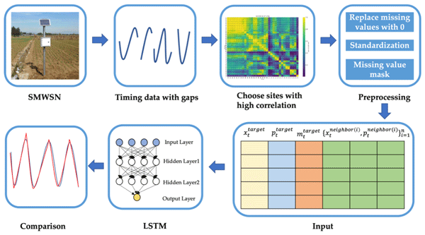
To achieve precise reconstruction of missing values, this study proposes the ST-GapFill framework. The experimental procedure of this paper is shown in Fig. 1.

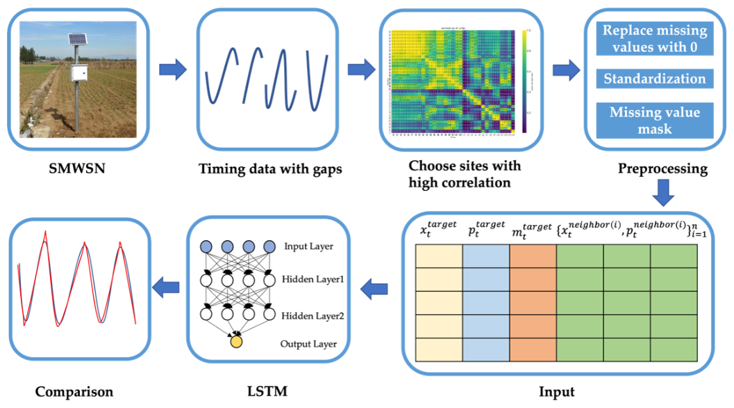
Figure 1 Experimental flowchart, showing the step-by-step process of the ST-GapFill method for missing data reconstruction.

2.1 Data pre-processing

Missing values in the original series were replaced with 0 and both SM and rainfall data were normalized before converting data into time-series samples.

$$\begin{array}{}\text{(1)}& x_{t,\mathrm{norm}}={\displaystyle \frac{x_t-\mathit{\mu }}{\mathit{\sigma }}},\end{array}$$

Here, μ and σ denote the sample mean and sample standard deviation of the training data, respectively, ensuring the normalization is consistent with the observed distribution.

The input data for the prediction model includes the target station and its selected neighboring stations, identified based on their strong spatial correlation. The features for each station include soil moisture (SM), precipitation (PP), and a missing value mask (0 for missing values, 1 for observed values). The target station data is used for prediction, while the neighboring stations' data help provide spatial context. The input to the model at time t can be expressed as the following vector:

$$\begin{array}{}\text{(2)}& \begin{array}{rl}{\mathit{X}}_t=& [x_t^{\mathrm{target}},p_t^{\mathrm{target}},m_t^{\mathrm{target}},\\ & \mathit{\{}{x}_t^{\mathrm{neighbor}\left(i\right)},p_t^{\mathrm{neighbor}\left(i\right)}{\mathit{\}}}_{i=\mathrm{1}}^n],\end{array}\end{array}$$

where n is the number of selected neighboring stations. $x_t^{\mathrm{target}}$, $p_t^{\mathrm{target}}$, $m_t^{\mathrm{target}}$ represent the normalized SM, normalized precipitation and missing value mask at the target station at time t. $x_t^{\mathrm{neighbor}\left(i\right)}$ and $p_t^{\mathrm{neighbor}\left(i\right)}$ represent the normalized SM and precipitation at neighboring stations i, respectively, for time t.

The output, or the target prediction for the target station at time t, is the SM value $y_t^{\mathrm{target}}$, which is predicted by the model. Thus, the relationship can be summarized as:

$$\begin{array}{}\text{(3)}& y_t^{\mathrm{target}}=f\left({\mathit{X}}_t\right),\end{array}$$

where f(⋅) represents the prediction function of the model (e.g., LSTM).

2.2 Correlation calculation

In gap-filling tasks, highly correlated stations enable the model to utilize more relevant information, thereby improving interpolation accuracy. To model the spatial dependence between sites in WSN, a Gaussian model is introduced to calculatethe spatial correlation between each pair of sites (Birgé and Massart, 2001). For stations with missing data, a correlation threshold is set. Sites with a correlation greater than this threshold are considered more correlated to the target site, and their features are fed into the model for interpolation (Ren et al., 2022).

$$\begin{array}{}\text{(4)}& {\displaystyle }\begin{array}{rl}& d=\mathrm{2}r\cdot \arcsin \\ & \left(\sqrt{{\sin }^{\mathrm{2}}\left({\displaystyle \frac{\mathrm{\Delta }\mathit{\varphi }}{\mathrm{2}}}\right)+\cos \left({\mathit{\varphi }}_{\mathrm{1}}\right)\cos \left({\mathit{\varphi }}_{\mathrm{2}}\right){\sin }^{\mathrm{2}}\left({\displaystyle \frac{\mathrm{\Delta }\mathit{\lambda }}{\mathrm{2}}}\right)}\right),\end{array}\text{(5)}& {\displaystyle }\mathrm{correlation}=\exp \left(-{\displaystyle \frac{d^{\mathrm{2}}}{L^{\mathrm{2}}}}\right),\end{array}$$

d is the distance between the two points; r is the radius of the Earth, typically taken as 6371 km. ϕ₁ and ϕ₂ are the latitudes (in radians) of the two points, respectively. λ₁ and λ₂ are the longitudes (in radians) of the two points. Δϕ is the latitude difference: (ϕ₂−ϕ₁). Δλ is the longitude difference: (λ₂−λ₁). d is the distance between the two sites and L is the scale parameter of correlation, where L=50 km. The scale parameter L=50 km was determined based on the spatial resolution of the SMN-SDR network (grid size of 1°×1° and empirical validation results. Additionally, a sensitivity analysis was performed by testing alternative values (30 and 70 km). The resulting variations in RMSE were less than 2 %, confirming that L=50 km provides a stable and representative spatial correlation threshold for the network.

2.3 Long short-term memory

Long Short-Term Memory (LSTM) is a variant of Recurrent Neural Networks (RNN). LSTM, proposed in 1997 by Schmidhuber and Hochreiter (Hochreiter and Schmidhuber, 1997), alleviates the problem of gradient vanishing in RNN models and is the most commonly used neural network for modeling time series in deep learning (Nelson et al., 2017). In this study, a temporal modeling framework tailored to the characteristics of missing SM data is designed. The network architecture comprises a Masking layer, a double-stacked LSTM, and a Dense output layer.

• Masking Layer: Ignores missing values padded with zeros in the input sequence, preventing invalid information from interfering with model learning.

• First Layer LSTM: Extracts local temporal dependencies and short-term fluctuations from the raw feature sequence, and outputs a complete sequence of hidden states.

• Second Layer LSTM: Receives the hidden state from the first layer to further capture higher-level temporal dependencies and long-term trends, enabling stronger sequential pattern representation capabilities.

• Dense Layer: Maps the extracted temporal features to the predicted values for the target site at the current time step, thereby outputting the regression results.

To leverage more contextual information, sliding window slicing is employed to construct training samples, enabling the model to capture sufficient temporal signals before and after long missing segments or block-like gaps. By jointly inputting target site and neighboring station data, the LSTM simultaneously learns temporal dependencies and spatial context, ultimately achieving high-precision missing value reconstruction.

3 Experiments

3.1 Data Description

Shandian River is located in Chicheng County, Hebei Province, at the headwaters of the East Monkey, the birthplace of the Luan River, which flows through the border zone between Hebei and Inner Mongolia. The climate of the basin is a continental monsoon climate, with an average annual precipitation of about 375 mm and an annual evaporation of 1188 mm. The soils are mainly sand-dune soils, accounting for 50 % of the total watershed area, followed by meadow soils, accounting for about 8 %. SM varies significantly in the region (Wen et al., 2021; Xie et al., 2021). The soils are relatively dry in spring due to strong monsoon winds and become moist in summer due to abundant precipitation.

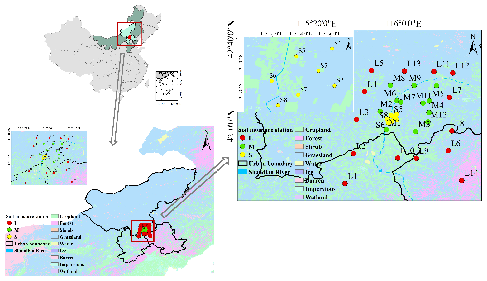
Figure 2 Schematic diagram of site locations, showing the 34 stations in the SMN-SDR network, with distinct scales for large (L), medium (M), and small (S) sites.

In 2018, an integrated remote sensing experiment of water cycle and energy balance was conducted in the Shandian River Basin (Zhao et al., 2020, 2021; Yan et al., 2021). The experiment is divided into three parts: airborne flight experiment, ground synchronized observation and ground parameter measurement. The data used in this paper are from the Soil Moisture Network Observations (SMN-SDR) in Shandian River Basin. SMN-SDR is a synergistic set of networks for observing soil temperature (TS), SM and precipitation (PP). It was established during the Luan River Soil Moisture Experiment from 18 July 2018 to 28 September 2018, covering an area of about 10 000 km² (115.5–116.5° E, 41.5–42.5° N) with a grid size of 1°×1°. Sensors at three distances of 100, 50, and 10 km were deployed in the SMN-SDR as shown in Fig. 2. The letters L, M, and S stand for large, medium, and small scales, respectively, and there were 34 stations. The soil moisture sensors used in the monitoring network were Decagon 5TM probes installed at depths of 3, 5, 10, 20, and 50 cm. The network consists of 34 monitoring sites, among which 20 sites are equipped with HOBO tipping-bucket rain gauges for precipitation measurements. Power for each station is supplied by solar panels, and all observations are transmitted wirelessly to a central server. Soil moisture and rainfall data were recorded at 10 min intervals prior to June 2019 and at 15 min intervals thereafter. In this study, rainfall observations were used as an auxiliary variable for the soil moisture gap-filling model because precipitation is a key driver of short-term soil moisture dynamics.

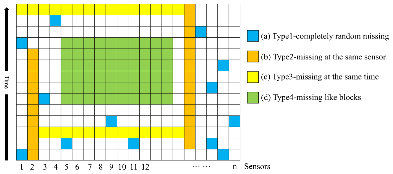
Figure 3 Patterns of missing values, illustrating the different types of missing data patterns in the SM network.

To ensure consistency and avoid introducing additional missing patterns, only SM at 3 cm depth and PP were used in this study. The shallow soil layer responds most rapidly to atmospheric forcing, particularly precipitation events, and therefore exhibits stronger temporal variability and more frequent missing observations. These characteristics make the 3 cm soil moisture series a more challenging and representative dataset for evaluating the performance of gap-filling methods. There are only 20 sites with PP. Considering the proximity of precipitation observations from neighboring sites, the geographically closest site was selected as a supplement to the missing rainfall data. There are missing values for up to 16 months in S1, so S1 was excluded from the experiment. All data from the remaining 33 sites were uniformly filtered from 1 January 2019 to 31 December 2020. Raw data were sampled at 10 or 15 min intervals. A method of taking averages was used to resample all data uniformly for 30 min.

3.2 Baseline algorithms

Autoregressive Integrated Moving Average Model (ARIMA): ARIMA is based on historical data of time series and fills the gaps by capturing the autocorrelation and randomness of the data. ARIMA transforms the existing non-stationary series into a stationary one through differencing to make it smooth. The autoregressive and moving average components are utilized to estimate the values of the missing data. Interpolation is performed based on the relationship between the previous and subsequent time points and the trend of the error term. Missing data that are consistent with the trend of the original series are generated (Shumway and Stoffer, 2017). The parameters of the ARIMA model were selected through grid search on the validation set with the aim of minimizing the Akaike Information Criterion (AIC). In the ARIMA (p, d, q) model, p, d, and q represent the orders of the autoregressive (AR), differencing (I), and moving average (MA) components, respectively. The range of p is 0–6, d is 0–2, and q is 0–6. Missing values were estimated by iteratively forecasting forward and backward using the ARIMA model, conditioned on observed data within the sliding window.

Inverse distance interpolation (IDW): IDW is a method of spatial interpolation based on the distance between a known data point and the point to be interpolated. The core principle is that the closer the known points are to the point being interpolated, the greater their influence, and the farther the known points are, the lesser their influence. The distance between each known point and the point to be interpolated is calculated and the inverse of the distance is used as weights. These weights are later used to perform a weighted average of the values of the known points. Finally, the estimated values of the points to be interpolated are obtained (Lu and Wong, 2008). For IDW, the inverse distance weighting power was set to 2, as it provided optimal results in prior SM interpolation studies (Dhevi, 2014).

Support Vector Regression (SVR): SVR models data based on its nonlinear relationships and is used to fill the gaps in time series or spatial data. SVR minimizes the error between the predicted value and the true value by mapping the input data to a high-dimensional space and finding the optimal hyperplane in that space. It also ensures that the model has good generalization ability. For missing values, SVR fits a smooth interpolation result based on known data points using support vector weights and kernel functions to achieve reasonable prediction and interpolation of missing data (Osman et al., 2021).

Last Observation Carried Forward (LOCF): LOCF is a simple time series interpolation method that maintains sequence continuity by carrying forward the most recent observation to fill missing positions. This method is straightforward to implement with minimal computational overhead, making it suitable for scenarios with short missing intervals and stable sequence changes. However, because LOCF assumes the variable remains unchanged during the missing period, it may underestimate or overestimate the magnitude of sudden changes and performs poorly in cases of long-term gaps or rapid fluctuations (Lachin, 2016).

3.3 Missing Patterns

Referring to the study of Li et al. (2019), the missing patterns of WSN can be categorized into three types: missing completely random (MCR), missing at random (MR), and non-MR (NMR).

In MCR, missing values may occur due to temporary power outages or communication failures. Therefore, they are completely independent. As shown in Fig. 3a, the missing values are some randomly scattered isolated points.

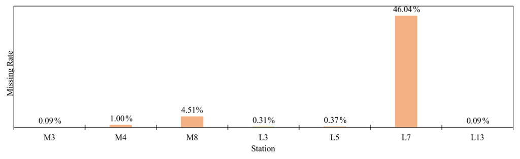
Figure 4 Missing rates of SM across all stations in the SMN-SDR network, highlighting stations with missing values exceeding 0.03 % (e.g., L3, L5, L7).

In MR, missing values may occur due to physical damage or maintenance backlog. Missing values are correlated with their temporally or spatially neighboring readings. As a result, such missing patterns are shown as a number of consecutive points at the same sensor (Fig. 3b) or at the same time (Fig. 3c).

In NMR, this missing pattern is usually caused by a long-term failure of the sensor and the missing values appear in certain patterns. As shown in Fig. 3d, the values are missing like blocks.

3.4 Experimental setup

To test the robustness of the proposed interpolation model, four missing data patterns are artificially injected into the dataset. To evaluate the stability of the model under different missing rates, the missing rates of the simulation experiments are set to [0.05, 0.1, 0.15, 0.2, 0.25, 0.3, 0.35, 0.4, 0.45, 0.5]. Sensors and timestamps were randomly selected when generating missing values to mimic the effect of filling in natural data.

To evaluate the model performance, the full dataset was randomly split into training (80 %) and testing (20 %) sets. Within the training set, 20 % of the samples were further used for validation. As a result, the final data allocation consisted of 64 % for training, 16 % for validation, and 20 % for testing. The input size is the total number of features. The batch size of the training data is set to 16 and the model repeats the training process 50 times on the training dataset to get the best performance of the model. The sliding window size for optimizing the performance of ARIMA, SVR and LSTM was set within the range of [50, 100, 150, 200, 250, 300].

The performance evaluation metrics include Mean Absolute Error (MAE), Root Mean Square Error (RMSE) and Coefficient of Determination R². The calculation method is as follows:

$$\begin{array}{}\text{(6)}& {\displaystyle }\mathrm{MAE}={\displaystyle \frac{\mathrm{1}}{N}}{\sum }_{i=\mathrm{1}}^n\mathrm{|}(y_i-{\widehat{y}}_i)\mathrm{|},\text{(7)}& {\displaystyle }\mathrm{RMSE}=\sqrt{{\displaystyle \frac{\mathrm{1}}{n}}{\sum }_{i=\mathrm{1}}^n(y_i-{\widehat{y}}_i{)}^{\mathrm{2}}},\text{(8)}& {\displaystyle }{R}^{\mathrm{2}}=\mathrm{1}-{\displaystyle \frac{{\sum }_{i=\mathrm{1}}^n(y_i-{\widehat{y}}_i{)}^{\mathrm{2}}}{{\sum }_{i=\mathrm{1}}^n(y_i-\stackrel{\mathrm{‾}}{y}{)}^{\mathrm{2}}}}\end{array}$$

y_i denotes the observed value, ${\widehat{y}}_i$ denotes the model's predicted value, n denotes the total number of samples, $\stackrel{\mathrm{‾}}{y}$ denotes the mean of the sample.

MAE directly calculates the absolute value between the true value and the predicted value. RMSE is the square root of the average squared differences between the true and predicted values, commonly used to assess the deviation between them. R² represents the degree of fit between the model's predicted values and the observed values. The smaller the RMSE and MAE are, the better the model performance.

4 Results and Discussion

4.1 Display of missing data

In this paper, the focus of the experiments is to discuss the effect of interpolation of the model in the presence of a large number of missing values. The model concentrates on modeling pairs of long intervals of consecutive missingness and deals with block missingness. The SM missing rates for sites that need to be interpolated are shown in Fig. 4. Each site had 35 089 pieces of data. More than 10 missing data were considered to be filled in. The number of missing values up to 10 was negligible, and sites with no missing values participated in the assumed experiments after replacing the missing values by taking the mean before and after. L3, L5, L7, L13, M3, M4, and M8 with missing values of 0.03 % or more were selected as actual sites to be interpolated. L1, L2, L4, L6, L8, L9, L10, L11, L12, and L14, which have no missing values, are selected as assumed sites. After introducing missing values for four missing patterns at every assumed sites, simulation experiments were conducted to test the stability of the model at different missing rates.

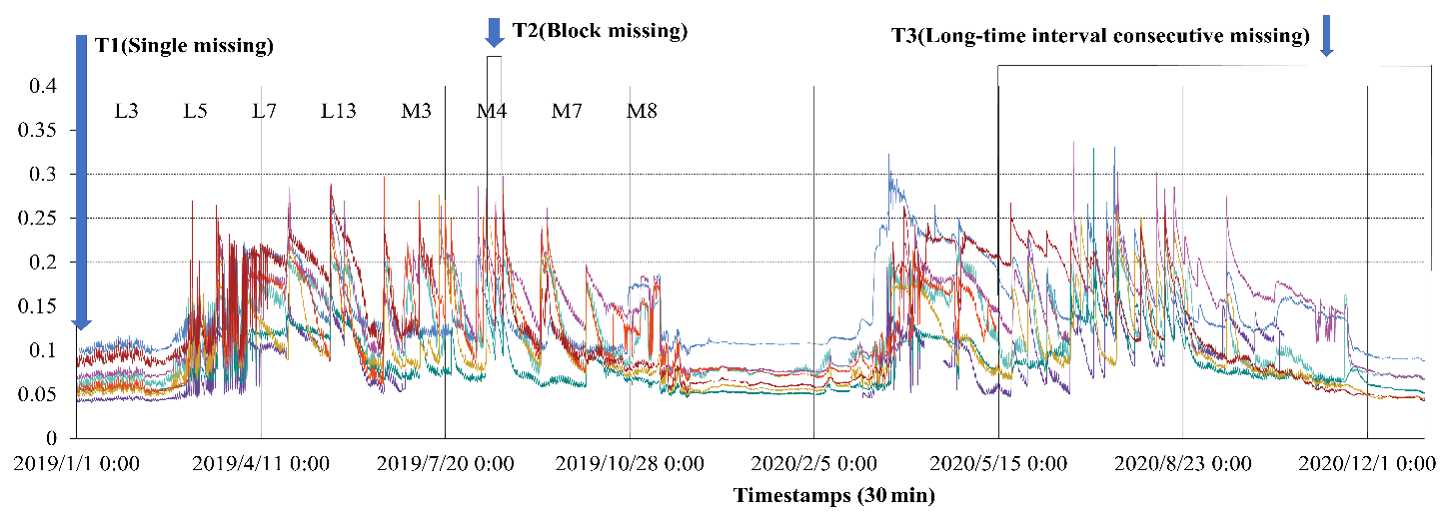
Figure 5 Missing SM time series under different missing patterns. A visual representation of soil moisture time series data showing the impact of different missing data patterns (MCR, MR, NMR) across multiple stations.

The selection of L3, L5, L7, L13, M3, M4, and M8 as imputation targets was driven by their significantly higher missing rates (exceeding 0.03 %) compared to other stations in the SMN-SDR network, as illustrated in Fig. 4. These sites exhibited diverse and severe missing patterns: L7 and M8, for instance, had missing rates of 46.04 % and 31.79 %, respectively, dominated by block missing (Type 4) or hybrid patterns (e.g., L7 combined Type 2 and Type 4), which posed substantial challenges for gap-filling algorithms. In contrast, stations like L1 and L2 had near-complete records and were used for controlled experiments where missing values were artificially introduced to validate the model's robustness across simulated scenarios (e.g., MCR, MR, NMR). The chosen targets also represented a strategic mix of spatial scales (large/L, medium/M), ensuring the evaluation covered varied hydrological responses to precipitation and evaporation. Their geographic distribution across the Shandian River Basin – a region with pronounced SM variability due to monsoonal climate – further allowed the model's performance to be tested under real-world complexities, such as abrupt moisture changes after rainfall or prolonged dry spells. By focusing on these high-missing-rate stations, the study prioritized practical correlation, as their reconstruction is critical for maintaining data continuity in long-term climate and hydrological analyses.

Figure 5 shows the missing SM time series. From Fig. 5, it can be seen that there are a large number of single random missing like T1 moments, i.e., MCR. At T2, the values of L7, M4, and M8 are missing, i.e., NMR. At T3, M7 was missing in its entirety, i.e., MR, accompanied by single missing values from other sites. The occurrence of missing values is completely random and unpredictable. Different missing patterns require different models, adding difficulty to the modeling task. So, the relationship between space and time needs to be considered when filling in missing values. When gaps occur at long intervals, it may result in a too small sample size to train the model. Meanwhile, it can be seen from Fig. 5 that the time series of the sites have a high degree of similarity, with similar periods and trends. Therefore, neighboring sites with higher correlation can be used to supplement the lack of features.

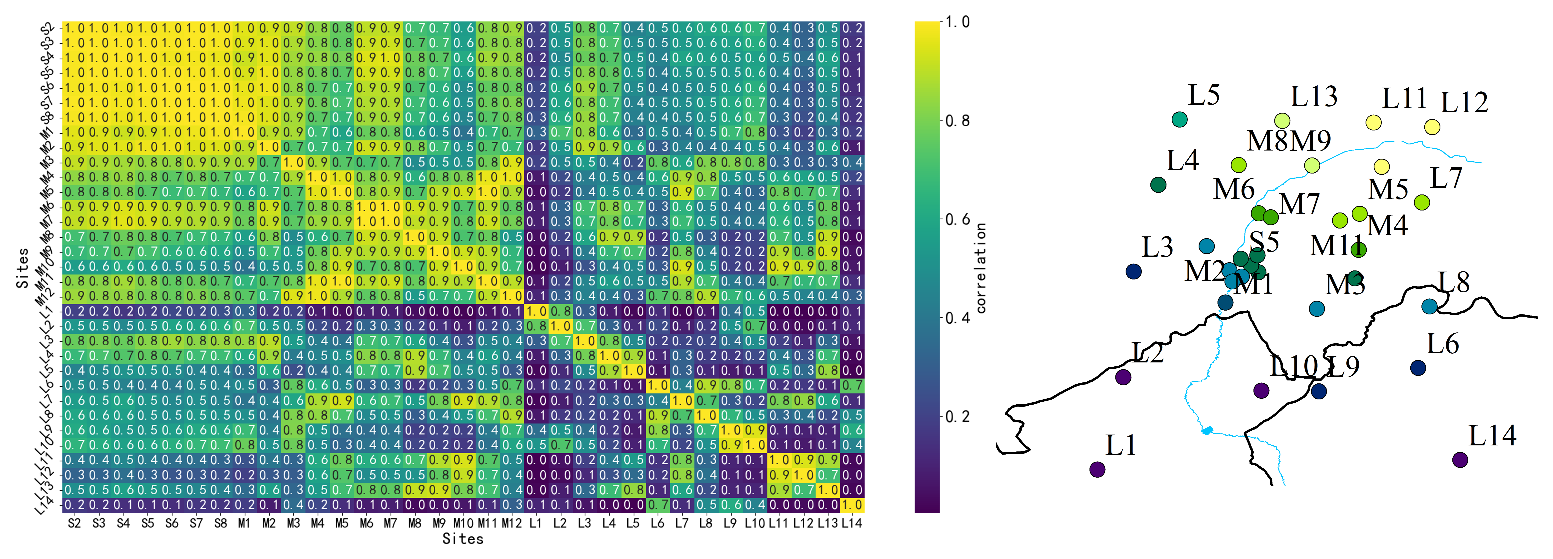
Figure 6 Correlation between sites (left) and geographic distribution of stations (right). The color of each dot represents its correlation with station L11, where yellow indicates strong correlation and dark blue indicates weak correlation.

4.2 Neighborhood sites selecting

The correlations between sites are shown in Fig. 6. As can be seen in Fig. 6, most of the correlations for the small-scale sites beginning with S are above 0.7, and some are even close to 1.0. These sites have similar environmental factors and are geographically close to each other. Most of the correlations between the M sites (M1 to M6) are between 0.6 and 0.8. The correlation between sites S (e.g., S5, S6) and M (e.g., M9, M10) is around 0.4 or even lower. Sites L, especially L6, L10, L11, have low correlation with most of the sites (mostly in the range of 0.2 to 0.5). Sites L13, L14 have very low correlation with the other sites, in the range of 0.2 to 0.5. The high correlation sites have similar trends in measured values and are influenced by common environmental factors. The information exchange between sites can make up for the shortcomings of their own features. With a threshold of 0.85, highly correlated sites will be combined as feature inputs to improve the prediction accuracy of the model.

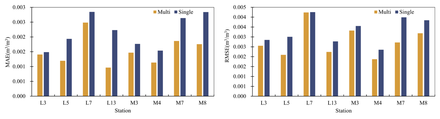
Figure 7 Comparison of accuracy before and after correlated sites joining, showing high correlations among nearby small-scale sites and varying correlations among larger sites.

The error shown in Fig. 7 is the comparison of accuracy before and after incorporating neighboring station information. The size of the uniform sliding window is 100, and a comparison test is performed for the actual sites L3, L5, L7, L13, M3, M4, and M8 that need to be interpolated. After adding the correlated sites, most of the sites show lower errors. In particular, L5, L13, M7, and M8 showed significant reductions in MAE and RMSE. L7 showed the highest error, with 14.5 % and 0.43 % reductions in MAE and RMSE. M7 and M8 showed similar trends, with MAE decreasing by 41.4 % and 46.6 %, and RMSE decreasing by 61.8 % and 20.7 %, respectively. L13 showed the most significant change, with MAE and RMSE decreasing by 131.3 % and 23.6 %, respectively. Some sites, such as L3, L7, and M3, did not have a large difference in MAE or RMSE between the two, but still had a slight advantage with the addition of the correlation site.

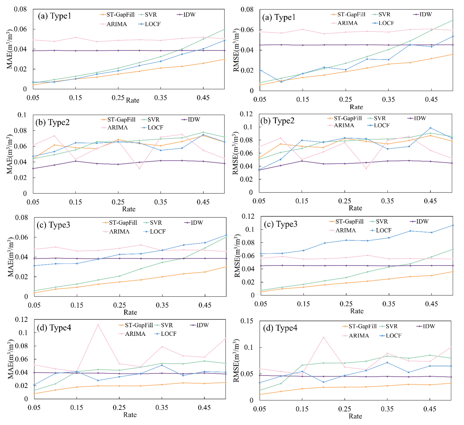
Figure 8 MAE and RMSE of models for different missing patterns, comparing the performance of various models (ST-GapFill, SVR, ARIMA, IDW, LOCF) under different missing data patterns.

4.3 Analysis of simulated data

After individual experiments with sliding window sizes of [50, 100, 150, 200, 250, 300], the optimal window sizes of 250 for ARIMA, 50 for ST-GapFill, and 50 for SVR were finally obtained, respectively. At the best sliding window size of each model, L1, L2, L4, L6, L8 with no missing values, L9, L10, L11, L12, and L14 sites were randomly introduced with missing values from the four missing models for a hypothesis experiment.

Figure 8 demonstrates the performance of different models with different missing rates for different missing modes. The trends of MAE and RMSE are the same. For the Type 1 pattern, SVR and ST-GapFill increase the error with increasing missing rate. However, among the four models, ST-GapFill consistently minimizes the error. IDW remained essentially constant, with its MAE and RMSE consistently around 0.038 and 0.045 m³ m⁻³. The error of SVR is greater than that of IDW when the missing rate reaches 40 %. For the Type 2 pattern, as the missing rate increases, the long succession of missing values leads to a decrease in the training samples, resulting in fluctuating variations in all four models. IDW consistently maintains the lowest MAE and RMSE. ARIMA has a wide range of fluctuations and is very unstable. For missing rates below 30 %, ST-GapFill and SVR perform similarly. After the missing rate is greater than 30 %, ST-GapFill is consistently lower than SVR by a small margin compared to SVR. For the Type 3 pattern, MAE and RMSE of IDW remained near 0.038 and 0.045 m³ m⁻³. Although the errors of ST-GapFill and SVR increase with increasing missingness, ST-GapFill consistently performs best and ARIMA performs worst. The error of SVR is higher than that of IDW at a missing rate of 40 %. MAE and RMSE of SVR are higher than those of ARIMA at a missing rate of 45 %. For the Type 4 pattern, as the missing rate increases, MAE and RMSE of the ST-GapFill are kept at the lowest level, although there is a small increase. The increase decreases after the deletion rate is greater than 15 %. MAE and RMSE of SVR are higher than those of IDW at a missing rate of 15 %. MAE and RMSE of IDW remained stable at 0.039 and 0.045 as usual. The R² values between the actual and predicted values are calculated in Fig. 9. Higher R² values indicate more consistent estimates. ST-GapFill produces higher correlation values for all missing models, except for IDW, which has the highest correlation for the Type 2 pattern. This indicates that the interpolations generated by ST-GapFill are more consistent with the actual values.

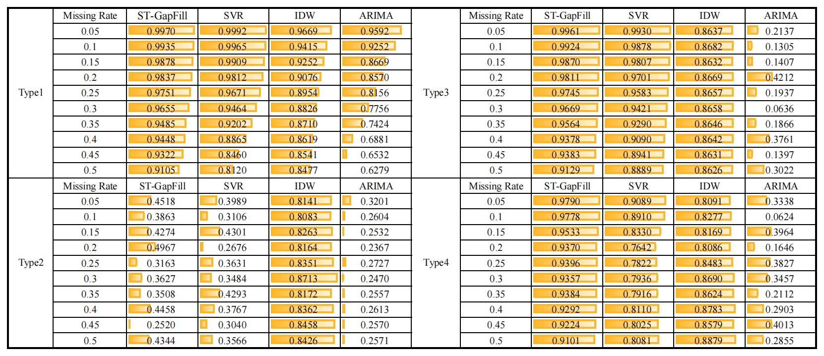
Figure 9 Comparison of coefficient of determination (R²) under different missing data types. Higher R² values indicate better consistency between predicted and observed soil moisture.

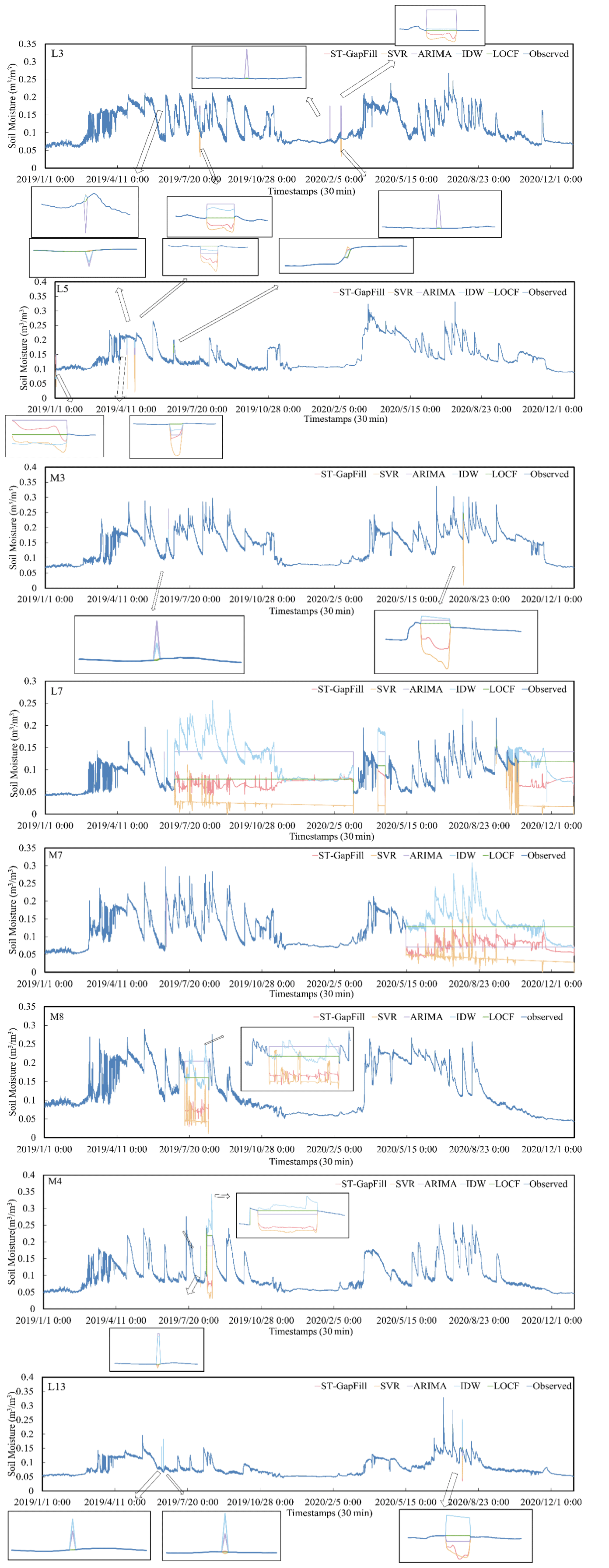
Figure 10 Timing changes after missing values are interpolated, comparing the results of ST-GapFill, IDW, ARIMA, LOCF and SVR for different missing rates.

To further refine baseline comparisons, we introduced LOCF and compared it with ARIMA, SVR, IDW, and ST-GapFill (Fig. 8). It can be observed that LOCF performs similarly to ARIMA and SVR when the missing rate is low (≤ 15%), and even slightly outperforms IDW in the Type 1 scenario. However, as the missing rate increases, LOCF's errors significantly grow, with particularly noticeable deterioration in Type 3 and Type 4 block missing scenarios. This occurs because LOCF cannot utilize information from time steps following the missing data, causing predicted values to remain stagnant at pre-missing levels and failing to reflect subsequent dynamic changes in humidity, whether declines or increases.

Based on the above analysis, several conclusions can be drawn. (1) For the Type 2 pattern (consecutive gaps at a single sensor), the spatial interpolation model IDW outperforms the temporal models (ST-GapFill, SVR, and ARIMA). This is because long consecutive gaps reduce available temporal training information, limiting the ability of LSTM-based models to reconstruct missing sequences, whereas IDW relies solely on contemporaneous spatial neighbors that remain available. (2) For the other missing patterns – Type 1 (random missing), Type 3 (simultaneous multi-sensor missing), and Type 4 (block missing) – ST-GapFill achieves the best overall performance, showing the lowest MAE and RMSE across missing rates. (3) As the missing rate increases beyond 40 %, all time-series-based models exhibit performance degradation, but ST-GapFill's error growth is slower than SVR's. (4) In particular, for Type 4 block missing, ST-GapFill demonstrates a distinct advantage, maintaining high reconstruction accuracy (MAE ≈ 0.038 m³ m⁻³, RMSE ≈ 0.045 m³ m⁻³) even when up to 50 % of the data are missing.

Overall, these results indicate that while ST-GapFill effectively leverages both temporal dependencies and spatial correlations, it performs best under missing scenarios where sufficient temporal context exists (Type 1, 3, 4). For Type 2, where consecutive gaps severely disrupt temporal continuity, IDW provides a more stable and robust alternative. Therefore, the two approaches are complementary: ST-GapFill excels in complex spatiotemporal contexts, while IDW remains preferable for persistent single-sensor outages.

In the analysis of simulated data, the ST-GapFill method demonstrated significant advantages over other traditional methods. For example, compared to spatial interpolation methods based on IDW, ST-GapFill introduces a dynamic spatial correlation selection mechanism to more accurately identify neighbouring sites with environmental dynamics similar to the target site. This method not only considers spatial proximity but also incorporates complex nonlinear relationships in time series, enabling more effective filling of data gaps when handling simulated data with high missing rates. Additionally, compared to ARIMA, ST-GapFill can better capture long-term dependencies in time series, particularly when handling nonlinear data, where its performance is even more prominent. This indicates that ST-GapFill has greater adaptability and accuracy when processing data with complex spatio-temporal dependencies.

Compared with existing studies, ST-GapFill has obvious advantages in processing data with high missing rates. Chen et al. (2020) used a spatiotemporal adaptive method, but its accuracy was limited by large-scale continuous missing data. Moreno-Martínez et al. (2020) used a multispectral high-resolution sensor fusion method, but its performance was limited when processing data with high missing rates and blocky missing data, while ST-GapFill dynamically selects relevant sites and uses an LSTM network to capture complex temporal dependencies, making it more effective at handling high-missing-rate block-missing data, with lower MAE and RMSE values.

Under low missing-rate conditions (< 10 %), the RMSE of 0.038 m³ m⁻³ approaches the Decagon 5TM sensor's intrinsic accuracy of ±0.03 m³ m⁻³ (manufacturer specification), indicating that the errors introduced by our gap-filling method are no greater than the inherent noise level of the sensor itself, suggesting that the reconstructed data can be considered highly reliable for practical applications. It is noteworthy that the RMSE and MAE values in Sect. 4.3 (0.03–0.05 m³ m⁻³) are significantly higher than those in Sect. 4.2 (typically < 0.01 m³ m⁻³). This is expected, as Sect. 4.2 uses complete observations and evaluates the effect of incorporating neighboring stations under no artificial gap conditions. In contrast, Sect. 4.3 involves simulated data gaps under four distinct missing scenarios, where temporal continuity is intentionally disrupted. Especially in NMR (non-missing at random) cases, the target station has no available data during the missing block, forcing the model to rely entirely on external spatial and historical features, which inevitably increases reconstruction error.

4.4 Analysis of in-situ data

In order to further verify the upper and lower limits of the ST-GapFill interpolation effect, interpolation was completed for the actual sites L3, L5, L7, L13, M3, M4, and M8 in the original dataset that needed to be interpolated, and the timing variations were plotted as shown in Fig. 10. The missing rate of less than 0.1 % was the lowest for M3 and L13, which were all of the Type 4 with block missing. The L3, L5, and M4 missing rates were 0.31 %, 0.37 %, and 1.00 %, respectively. L3 and M4 were Type 4 pattern, and L5 was a Type 2 pattern. From the figure, it can be seen that ST-GapFill can better follow the trend of the data and is closer to the actual observations when the missing rate is small. ARIMA deviates from the observations. IDW performs smoothly and does not reflect the volatility of the SM well. SVR performs well in some interpolated regions but may be too smooth to capture the abrupt changes and details in the observed data well. The missing rate of M8 is 4.51 %, which is a block missing. From the figure, the temporal changes of IDW are articulated too smoothly, and ST-GapFill performs smoothly and is better able to keep in line with the observed data. M7 and L7 have the highest missing rates of 31.79 % and 46.04 %, respectively, and both are the combinations of the Type 4 missing pattern and the Type 2 missing pattern. ST-GapFill's interpolation results are more consistent with the fluctuating trends in the data, but it performs slightly more conservatively in the time period after August 2020 at site L7, and does not capture the dramatic fluctuations in the observed data. IDW performs well in the long missing time periods, but it does not reflect the fluctuating trends in the data very well. IDW may provide reasonable estimates in areas where SM is more stable or less variable, but it performs mediocrely in areas of high fluctuation. The interpolated results of SVR are significantly low, and ARIMA deviates completely from the trend of the actual observed data. Overall, LOCF produces step-like flat predictions at sudden drops or spikes, lagging significantly behind actual changes and exhibiting substantial reconstruction errors for long gaps. In contrast, ST-GapFill and SVR capture trend changes, delivering dynamic predictions closer to observations.

In the analysis of in-situ data, the ST-GapFill method also demonstrates its unique advantages. Compared with traditional interpolation methods, ST-GapFill can better reflect the actual trends in SM. For example, when handling data with low missing rates, ST-GapFill can more closely match actual observational values, indicating its high precision in handling small-scale data gaps. Furthermore, even in cases of high data missing rates, ST-GapFill can effectively fill data gaps, outperforming IDW and ARIMA. This indicates that ST-GapFill not only maintains data continuity but also more accurately reflects the dynamic changes in SM when processing actual observational data.

From a practical application perspective, ST-GapFill offers significant advantages over other methods. For example, Kang et al. (2019) proposed a data-driven method for filling long-term flux data gaps. Heaton et al. (2019) proposed a method based on non-Gaussian spatial and spatiotemporal data modelling. Both of these methods are limited by high-missing-rate block-wise missing data. In contrast, ST-GapFill maintains low MAE and RMSE values when handling block-wise missing data with high missing rates, indicating its significant advantage in handling complex spatio-temporal data. This superiority arises from the dynamic spatial correlation selection, which adaptively screens auxiliary stations (Birgé and Massart, 2001), and the iterative LSTM-based temporal fusion that preserves diurnal variability better than static interpolation or single-model approaches. These findings demonstrate that integrating multi-source contextual information can bridge longer missing blocks without sacrificing short-term fluctuation fidelity.

5 Conclusion

To reconstruct the missing data from the SM automatic monitoring station, this study presents ST-GapFill, the first hybrid model to jointly leverage adaptive spatial correlation screening and LSTM-based temporal modeling for soil moisture gap filling. Its key contributions are:

• Dynamic Spatial Correlation: By replacing fixed-distance neighborhood selection (e.g., IDW) with a Gaussian correlation model, ST-GapFill prioritizes environmentally similar sites, reducing noise from irrelevant sensors. This is particularly effective in heterogeneous landscapes (e.g., Shandian River Basin with mixed soil types).

• Iterative Multi-source Learning: The rolling window framework allows iterative prediction of long missing blocks (up to 50 % missing rate) by fusing temporal SM trends, precipitation signals, and spatial correlations. This outperforms static matrix completion methods (Rivera-Muñoz et al., 2022) that assume low-rank data structures.

• Superiority in Block Missing: The experimental results show that when the missing rate reaches 40 %, ST-GapFill still maintains a low MAE and RMSE of 0.038 and 0.045 m³ m⁻³, respectively. For block missing (Type 4), ST-GapFill significantly outperforms the other models, being able to maintain low MAE and RMSE with missing rates as high as 50 %. In contrast, traditional interpolation methods and other machine learning models perform less effectively in the case of high missing rates.

In the validation of real data, ST-GapFill demonstrates good performance. By comparing results with the LOCF baseline, we validate that simple temporal interpolation serves as a fast and effective solution in scenarios with low missing rates. However, its performance significantly degrades under high missing rates and complex missing patterns. When the missing rate is low, ST-GapFill can effectively capture the dynamic changes of SM, which are highly consistent with the actual observations. For example, the missing rates of L3 and L5 are low, and the interpolation results match closely with the actual data. And at sites M7 and L8, where the missing rate is high, ST-GapFill outperforms the traditional IDW and ARIMA models, even though it fails to fully capture the sudden fluctuations. This study not only confirms the effectiveness of ST-GapFill in missing time series data filling, but also provides an important theoretical basis for the development of future SM monitoring techniques.