Identifying dominant parameters in SWAT across subbasin and HRU scales using a two-step deep learning-assisted spatial sensitivity analysis

Distributed hydrological models require sensitivity analyses that explicitly account for spatial heterogeneity, yet such analyses are often constrained by high computational demands. This study presents a two-step, deep learning-assisted spatial sensitivity analysis (SSA) framework to identify dominant parameters across multiple spatial scales. Using the Soil and Water Assessment Tool (SWAT) in the Jinghe River Basin as a case study, the Morris method was first applied with a spatially lumped strategy to screen influential parameters. Subsequently, SSA was conducted using the Sobol' method with multilayer perceptron (MLP) surrogates to evaluate parameter sensitivities under both subbasin- and hydrologic response unit (HRU)-scale parameterizations. The surrogate models emulated SWAT with high accuracy for 195 subbasin-scale and 2559 HRU-scale parameters, enabling efficient estimation of Sobol' sensitivity indices. Results reveal pronounced spatial heterogeneity in parameter sensitivities. Sensitivity hotspots are consistently concentrated in gauge-proximal subbasins, while HRU-scale analysis further resolves localized controls. Robustness analyses demonstrate that the identified sensitivity patterns remain stable across different performance metrics, NSE-constrained posterior parameter distributions, alternative observation configurations, and varying numbers of screened parameters. These findings confirm the reliability of the proposed two-step framework and highlight its capability to efficiently diagnose dominant hydrological controls in high-dimensional distributed models. The methodology provides a transferable and computationally feasible approach for sensitivity assessment, supporting scale-aware calibration and improving the interpretability and predictive reliability of distributed hydrological simulations.

1 Introduction

1 Introduction

Runoff simulation underpins hydrologic prediction and decision-making, supporting applications ranging from short-term flood warnings (Su et al., 2024; Ou et al., 2025) and water allocation to ecosystem management (Dalcin and Fernandes Marques, 2020; Bai et al., 2025) to climate-adaptation planning (Hou et al., 2022; Zhou et al., 2023; Chitsaz et al., 2025). The reliability of these simulations depends critically on how hydrologic models transform rainfall into runoff. Broadly, such models fall into two classes according to their degree of spatial discretization: lumped and distributed (including semi-distributed variants) formulations (Fatichi et al., 2016; Pelletier and Andréassian, 2022; Bhanja et al., 2023). Lumped models treat the entire catchment as a single or a few effective units, providing computational efficiency and requiring fewer parameters, but at the cost of neglecting spatial heterogeneity in land surface characteristics. Distributed models, by contrast, explicitly account for spatial variations in soil, land cover, and topography by partitioning the basin into Hydrological Response Units (HRUs) or grid cells with spatially varying parameters. This enhanced realism improves process representation and transferability across basins but introduces high-dimensional parameter spaces and substantial computational burden. Because not all parameters exert equal influence across space, identifying where and to what extent individual parameters control model responses becomes essential for understanding and improving hydrologic simulations. Furthermore, distributed hydrologic models may adopt parameterizations at different spatial scales, such as subbasin and HRU levels, which influence how parameter sensitivities are represented and interpreted (Saint-Geours et al., 2014). Consequently, a key scientific challenge arises: how do parameter effects vary across space, and how do spatial scales reshape the sensitivity structure of distributed hydrological models?

Sensitivity analysis (SA) provides a systematic framework to quantify how variations in input parameters affect model output. In distributed runoff modelling, SA helps identify dominant parameters, guide calibration, and enhance process understanding. Conventional SA approaches applied to distributed hydrologic models can be grouped into spatially lumped and spatially distributed methods. Spatially lumped SA assumes uniform parameters or uniform scaling factors across the basin, offering computational efficiency but masking spatial heterogeneity (Zhang et al., 2013; Khorashadi Zadeh et al., 2017; Koo et al., 2020; Acero Triana et al., 2025). In contrast, spatially distributed SA (SSA) quantifies sensitivity at each spatial unit, revealing spatial patterns of hydrologic control and identifying sensitivity hotspots where certain parameters dominate (Tang et al., 2007; van Werkhoven et al., 2008; Rouzies et al., 2023). Beyond revealing spatial patterns of parameter influence, a key advantage of SSA is its ability to evaluate sensitivities across multiple spatial scales. Changes in spatial resolution can alter hydrologic connectivity, parameter aggregation, and process representation, thereby reshaping the magnitude and distribution of parameter sensitivities (Saint-Geours et al., 2014). Consequently, sensitivity patterns may vary substantially across spatial resolutions, reflecting the scale dependence of dominant hydrologic controls.

Despite its advantages, SSA faces a major challenge associated with the high dimensionality of distributed models. When parameters are defined at multiple spatial units, the total number of variables increases multiplicatively, often equalling the number of model parameters multiplied by the number of spatial units (Wu et al., 2022). As a result, hundreds or even thousands of distributed parameters may require evaluation. This rapid expansion of the parameter space leads to the so-called “curse of dimensionality,” which substantially increases computational demands and complicates uncertainty quantification (Razavi et al., 2012; Herman et al., 2013a).

Recent advances in surrogate modelling have provided promising solutions for reducing the computational demands associated with high-dimensional distributed models. Machine learning techniques, particularly deep neural networks, have been successfully employed to emulate complex hydrological models with high accuracy and significantly reduced computational cost (Razavi et al., 2012; Furong and Hossain, 2023; Jahanshahi et al., 2025; Yu et al., 2024). These approaches enable efficient exploration of high-dimensional parameter spaces and facilitate variance-based sensitivity analysis in distributed models. Nevertheless, few studies have systematically integrated deep learning surrogates with spatial sensitivity analysis to investigate how parameter importance varies across spatial scales while preserving the native parameterization structure of distributed models.

To address these challenges, this study develops a two-step, deep learning-assisted spatial sensitivity analysis framework based on the Soil and Water Assessment Tool (SWAT). The workflow consists of three main steps: (1) applying the Morris method to screen influential parameters associated with runoff simulation; (2) constructing multilayer perceptron (MLP) surrogates at both the subbasin and HRU scales to emulate SWAT; and (3) conducting SSA using the Sobol' method with the screened parameters to quantify spatial patterns of parameter influence. This framework enables computationally efficient global sensitivity analysis while explicitly preserving distributed parameter structures. The methodology is applied to the Jinghe River Basin, a typical semi-arid watershed in northwest China characterized by pronounced topographic gradients and substantial spatial heterogeneity. Specifically, this study aims to: (1) develop a computationally efficient framework for spatial sensitivity analysis in distributed hydrological models; (2) identify dominant parameters and their spatial distributions controlling runoff generation; and (3) quantify how spatial scale influences sensitivity patterns at subbasin and HRU resolutions. By achieving these objectives, this research advances understanding of how distributed parameters jointly control hydrologic responses across spatial scales, thereby enhancing the diagnostic capability, calibration efficiency, and predictive reliability of physically based hydrological models.

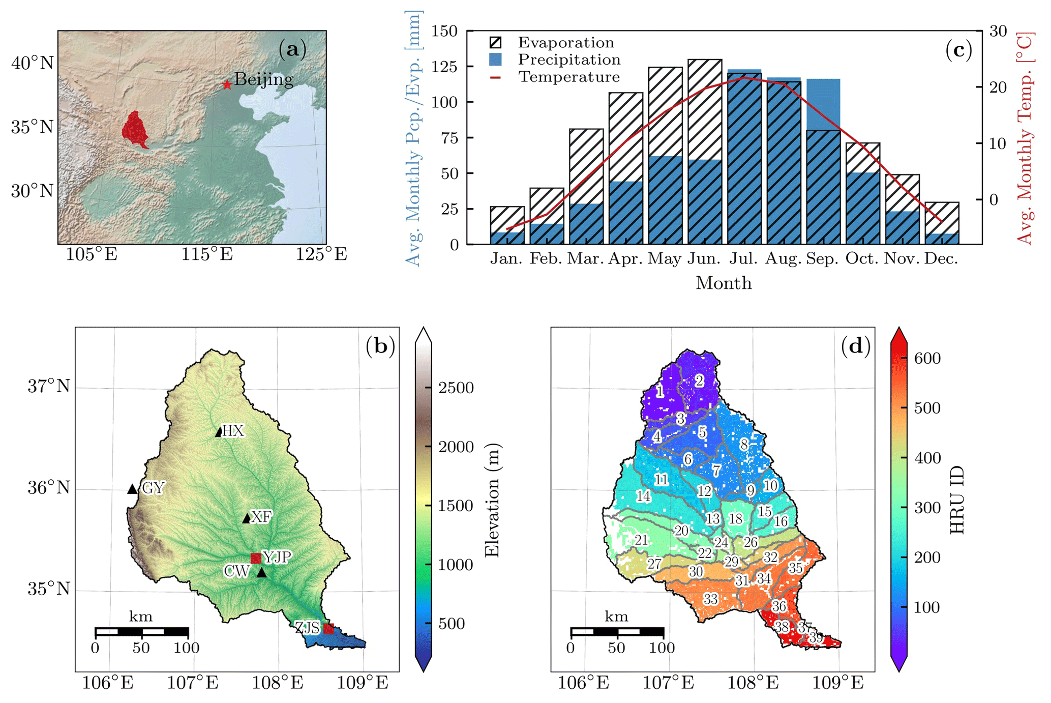
Figure 1 (a) Location of the Jinghe River Basin. (b) Basin topography based on the DEM obtained from the Geospatial Data Cloud (http://www.gscloud.cn/, last access: 5 April 2026). Black triangles denote four meteorological stations Huanxian (HX), Guyuan (GY), Xifeng (XF), and Changwu (CW), and the two red squares mark the Yangjiaping (YJP) and Zhangjiashan (ZJS) gauge stations. (c) Monthly mean climate characteristics during 1962–1986, including temperature (red line), precipitation (blue bars), and evaporation (black hatches). (d) Delineation of 39 subbasins and 630 HRUs. Numbers label subbasin IDs; colours indicate HRU IDs. Note a few subbasin labels are omitted to avoid overlap.

2 Methodology

2.1 Study area

The Jinghe River Basin, located in the central Loess Plateau of China, drains an area of 4.4 × 10⁴ km² from 34°46^′ to 37°19^′ N and 106°14^′ to 108°42^′ E (Fig. 1a). The mainstem is ∼ 455 km long and discharges to the Wei River (the largest tributary of the Yellow River). The basin typifies an agriculture-dominated region situated in the transition zone between semi-humid and semi-arid climates, characterized by severe soil erosion (Bai et al., 2022), fragile ecosystems (Xu et al., 2022), and high hydrological variability (Chang et al., 2016; Liu et al., 2024). The regional climate is strongly influenced by the East Asian monsoon, producing pronounced seasonality in rainfall. Daily records from four meteorological stations (Fig. 1b) during 1962–1986 indicate a mean annual temperature of 8.9 °C. Annual precipitation ranges from 381 to 857 mm, with a mean annual precipitation of 654 mm. Nearly 55 % of rainfall occurs between July and September. Mean annual potential evapotranspiration during 1962–1986, estimated by using the Penman-Monteith method, is 972 mm. Evapotranspiration exceeds precipitation from October through June of next year when rainfall is scarce (Fig. 1c).

In terms of topography, the elevation declines from northwest to southeast, from 2884 to 219 m above sea level (Fig. 1b). Consistent with this gradient, flow routes from the uplands in the northwest to the Wei River confluence in the southeast. Long-term (1956–2001) mean annual runoff was estimated at 8.36 × 10⁸ m³ at the Yangjiaping (YJP) gauge station and 19.98 × 10⁸ m³ at the Zhangjiashan (ZJS) station (Fig. 1c), with ∼ 55 % of the annual discharge occurring between July and October (Li et al., 2015). Land cover is dominated by cropland and pasture (82.2 %; Fig. S1a in the Supplement). Calcaric cambisols are the prevailing soil group, covering 67.9 % of the basin (Fig. S1b). The interplay of intensive cultivation, highly erodible loess, and uneven precipitation creates persistent challenges for ecological sustainability and robust hydrologic modelling, motivating sensitivity analyses that resolve controls across spatial and temporal scales.

2.2 Morris and Sobol' methods for global sensitivity analysis

The Morris method, also known as the Elementary Effects (EE) method (Morris, 1991), provides an efficient, qualitative screening of influential parameters (Gao and Bryan, 2016; Wu et al., 2022). Let the model output be y(x), with x = $(x_{\mathrm{1}},x_{\mathrm{2}},\mathrm{\dots },x_k)$ the vector of k uncertainty parameters. Each parameter is mapped to the unit interval [0,1] (e.g., by using its cumulative distribution), which is then discretized into p evels, yielding a perturbation step size of $\mathit{\delta }=\mathrm{1}/(p-\mathrm{1})$. For a randomly selected base point on this p-level hypercube grid, the EE of x_i (denoted as EE_i) is computed by a one-at-a-time perturbation of size δ with ($x_i+\mathit{\delta })\in [\mathrm{0},\mathrm{1}]$, while holding other parameters fixed (Yang and Ye, 2022):

$$\begin{array}{}\text{(1)}& {\text{EE}}_i={\displaystyle \frac{y(x_{\mathrm{1}},\mathrm{\dots },x_i+\mathit{\delta },\mathrm{\dots },x_k)-y(x_{\mathrm{1}},\mathrm{\dots },x_i,\mathrm{\dots },x_k)}{\mathit{\delta }}}.\end{array}$$

Repeating this perturbation from multiple random base points yields multiple EE_i values, from which three statistics are derived: the mean (μ_i) of EE_i, the standard deviation (σ_i) of EE_i, as well as the mean (${\mathit{\mu }}_i^{\ast }$) of |EE_i|. Following Campolongo et al. (2007), ${\mathit{\mu }}_i^{\ast }$ is preferred for identifying influential parameters because it avoids cancellation of effects with opposite signs. The σ_i reflects the dispersion of elementary effects and is used to detect parameters whose influence on the output is nonlinear or involves interactions with other parameters (Yang and Ye, 2022). Parameters with low ${\mathit{\mu }}_i^{\ast }$ and σ_i are considered non-influential and can be excluded from further analysis (Sreedevi and Eldho, 2019; Dai et al., 2024).

Equation (1) suggests that estimating a total of r EEs requires a total of 2rk model simulations, since each EE needs a base and a perturbed evaluation. Morris (1991) proposed a trajectory-based design to reduce this cost. Starting from a random base point, the design applies k successive one-at-a-time perturbations, each modifying a single parameter, to construct a trajectory of (k+1) points. Repeating this process r times yields r trajectories and a total of $r\times (k+\mathrm{1})$ model evaluations. This design substantially lowers the computational cost compared with the naive scheme, but its results remain qualitative.

To move from qualitative screening to quantitative ranking, we use the Sobol' method. The Sobol' method (Sobol', 2001; Saltelli et al., 2007) addresses this need by decomposing the total variance of model output into contributions from individual parameters and their interactions. For a model output y(x), Sobol' sensitivity indices give a rigorous measure of parameter sensitivity. The first-order sensitivity index S_i measures the main effect of a parameter x_i, and the total-effect sensitivity index S_Ti quantifies both the main effect and all interactions (Saltelli et al., 2007):

$$\begin{array}{}\text{(2)}& {\displaystyle }& {\displaystyle }{S}_{\mathrm{i}}={\displaystyle \frac{{\text{Var}}_{{\mathit{x}}_i}\left[E_{{\mathit{x}}_{\sim i}}\right(y\mathrm{|}{x}_i\left)\right]}{\text{Var}\left(y\right)}},\text{(3)}& {\displaystyle }& {\displaystyle }{S}_{\text{Ti}}={\displaystyle \frac{E_{{\mathit{x}}_{\sim i}}\left[{\text{Var}}_{{\mathit{x}}_i}\right(y\mathrm{|}{\mathit{x}}_{\sim i}\left)\right]}{\text{Var}\left(y\right)}},\end{array}$$

where E(⋅) and Var(⋅) denote the mean and variance, respectively; x_∼i represents all parameters except x_i. According to Saltelli et al. (2007), S_i supports “Factors Prioritization” by ranking parameters according to their direct importance, whileS_Ti supports “Factors Fixing” by identifying parameters that can be fixed without significantly affecting model output.

In practice, efficient estimation of Sobol' S_i and S_Ti follows the Saltelli's sampling scheme (Saltelli et al., 2007). The procedure begins with the generation of two independent sampling matrices, A and B, both of size N × k, representing N samples and k input parameters. Then for the ith parameter, a hybrid matrix C_i is formed by replacing the ith column of matrix B with the corresponding column from A. In other words, C_i is a copy of B except for that the ith column is taken from A. The S_i and S_Ti indices for all k parameters are then estimated simultaneously using 2× N model simulations from A and B, plus k×N model simulations from the hybrid matrices C_i, resulting in a total cost of $N\times (k+\mathrm{2})$ model runs (Yang et al., 2024). Although this remains computationally demanding, it provides a robust quantitative basis for parameter importance. This estimator is widely adopted in modern SA toolkits, including SALib (Herman and Usher, 2017) and the SAFE Toolbox (Pianosi et al., 2015).

2.3 SWAT model description and configuration

SWAT is a semi-distributed hydrological model that simulates water, nutrient, and pesticide transport at the catchment scale (Zhang et al., 2014; Aloui et al., 2023). In SWAT, a watershed is typically divided into spatially referenced subbasins to represent the heterogeneity of hydrological processes. Each subbasin is further subdivided into HRUs, defined by unique combinations of land use, soil type, and slope class (Golmohammadi et al., 2017; Jeong et al., 2024), and they constitute the smallest computational units within the model (Arnold et al., 2012). Although they are not spatially contiguous or explicitly georeferenced within a subbasin, each HRU is assumed to be internally homogeneous with respect to land surface characteristics that govern hydrological processes. All hydrological processes are driven by the soil-water balance, which is governed by (Neitsch et al., 2011):

$$\begin{array}{}\text{(4)}& \begin{array}{rl}{\text{SW}}_{\mathrm{t}}=& {\text{SW}}_{\mathrm{0}}+{\sum }_{i=\mathrm{1}}^t(R_{\text{day},i}-Q_{\text{surf},i}-E_{\mathrm{a},i}\\ & -W_{\text{seep},i}-Q_{\text{gw},i}),\end{array}\end{array}$$

where SW_t and SW₀ are the final and initial soil water content (mm), R_day,i is daily precipitation (mm) on day i, Q_surf,i is surface runoff (mm) on day i, E_a,i is evapotranspiration (mm) on day i, W_seep,i is water percolation from the soil profile into the vadose zone (mm) on day i, and Q_gw,i is groundwater return flow (mm) on day i.

A variety of datasets were prepared to configure the SWAT model for the Jinghe River Basin, as detailed below:

• 1.

  The DEM was derived from the ASTER GDEM V2 with a spatial resolution of 30 m, obtained from the Geospatial Data Cloud (http://www.gscloud.cn/, last access: 5 April 2026). It was used to delineate watershed boundaries, extract river networks and subbasins, and determine slope classes.

• 2.

  The soil map was obtained from the Harmonized World Soil Database (HWSD) at a spatial resolution of 1 km, available through the National Cryosphere Desert Data Center (https://www.ncdc.ac.cn/portal/, last access: 5 April 2026).

• 3.

  The land use map for 1980, with a spatial resolution of 30 m, was provided by the Geographical Information Monitoring Cloud Platform (http://www.dsac.cn/, last access: 5 April 2026). This dataset was chosen to reduce the influence of human impacts, such as the major soil and water conservation programs (e.g., the “Grain-for-Green” project) since the 1980s (Chen et al., 2007).

• 4.

  Monthly runoff records from the YJP and ZJS gauge stations (Fig. 1c), covering the period of 1962–1986, were retrieved from the National Earth System Science Data Center (http://www.geodata.cn/, last access: 5 April 2026).

• 5.

  Daily meteorological observations, including precipitation, air temperature, relative humidity, and wind speed were collected from four meteorological stations (Fig. 1c), via the Shaanxi Provincial Meteorological Bureau (http://sn.cma.gov.cn/, last access: 5 April 2026) for the period of 1962–1986. Solar radiation was not directly measured and was estimated using SWAT's built-in weather generator.

To reduce computational cost while preserving basin geometry, the effects of DEM and land use resolutions on HRU delineation were evaluated (Fig. S2 in the Supplement). The results indicate that HRU numbers are primarily controlled by DEM resolution, decreasing significantly as the DEM becomes coarser, whereas land use resolution has a comparatively minor influence. Moreover, the delineated number of subbasins and the watershed area remain essentially unchanged when the DEM resolution varies between 30 and 150 m. Therefore, the DEM and land use data were resampled to 150 and 3000 m, respectively, representing an optimal balance between preserving key hydrological features and ensuring computational efficiency. Using a drainage-area of 80 000 ha, the watershed was delineated into 39 subbasins. These subbasins were subdivided into 630 HRUs using the multiple HRUs option in SWAT by overlaying soil, land use, and slope maps, with thresholds of 10 % for soil, 15 % for land use, and 10 % for slope (Fig. 1d). Note that there are blank areas during the HRU generation process (Fig. 1d), which correspond to areas filtered out by these thresholds or to small spatial mismatches among layers. The full subbasin-HRU crosswalk is provided in Table S1 in the Supplement.

The model was executed at a daily time step over 1962–1986, consistent with the daily meteorological inputs. Since observed runoff was available only at the monthly scale, simulated daily runoff was aggregated to monthly values for model evaluation and SA. The first 10 years (1962–1971) were used as a warm-up period, and the subsequent 15 years (1972–1986) were analysed for sensitivity and evaluation. Rainfall-runoff processes were simulated using the Soil Conservation Service (SCS) Curve Number (CN) method and channel flow routing was represented by the variable storage method (Neitsch et al., 2011).

2.4 Parameter screening using the Morris method

The SWAT model contains a large number of parameters, potentially hundreds, depending on spatial discretization and the complexity of represented hydrological processes. Conducting spatial sensitivity analysis across the full parameter space is computationally infeasible, making preliminary screening necessary to identify the most influential parameters governing runoff dynamics. Guided by prior studies, we selected 33 parameters commonly recognized as important for runoff generation in SWAT (Table S2 in the Supplement). All parameters were assumed to follow uniform distribution within their corresponding uncertainty ranges, which were drawn from previous studies (e.g., Khorashadi Zadeh et al., 2017), or recommended ranges in the Theoretical Documentation of SWAT (Neitsch et al., 2011).

Table 1 Description of the five parameters screened by the Morris method.

^∗ CN2 is perturbed by “factor” approach to account for spatial variability. The other four parameters are perturbed using the “replace” approach. All parameters are assumed to follow the uniform distribution.

To reduce parameter dimensions while preserving dominant hydrological controls, a spatially lumped parameterization strategy was adopted during the screening step. Specifically, instead of perturbing each spatial instance independently at subbasin or HRU level, each parameter was controlled by a single basin-wide perturbation applied consistently across all spatial units. Two perturbation approaches were implemented based on parameter characteristics (Table S2). For parameters representing basin-wide or process-based thresholds (e.g., snowfall temperature, SFTMP), values were directly replaced with a uniform value across the watershed (the “replace” approach). In contrast, for parameters with inherent spatial heterogeneity, such as soil- and land-use-related variables (e.g., CN2 and SOL_BD), a multiplicative scaling factor was applied to their original spatially distributed values (the “factor” approach). These parameterization schemes are widely adopted in SWAT calibration and sensitivity studies to reduce dimensionality while preserving the underlying spatial structure of model inputs (Li et al., 2021; Mao et al., 2024).

Parameter sensitivity was then evaluated using the Morris method, with the Nash–Sutcliffe Efficiency (NSE) between observed and simulated monthly runoff at the ZJS gauge station for the period 1972–1986 (180 months) serving as the primary performance metric. The ZJS station was selected because it is located near the watershed outlet and therefore integrates the cumulative hydrological response of upstream processes. To assess the robustness of the sensitivity results, complementary performance metrics, including percent bias (PBIAS) and Kling-Gupta Efficiency (KGE), as well as alternative parameter distributions and observations from the YJP station, were further examined and discussed in the Discussion section.

A total of 500 trajectories were generated, resulting in 17 000 = 500 × (33+1) SWAT simulations. This number is substantially higher than that used in many typical Morris applications and was deliberately selected to enhance the robustness of the screening step (Fig. S3 in the Supplement). For each run, the SWAT model was executed, and the NSE was computed between the simulated and observed monthly runoff at ZJS station over the 180-month period. The Morris method was then used to calculate ${\mathit{\mu }}_i^{\ast }$ and σ_i for each parameter, and a scatterplot of ${\mathit{\mu }}_i^{\ast }$ versus σ_i was used to screen the influential parameters (Yang and Ye, 2022). This procedure screened five dominant parameters: CN2, CANMX, ESCO, CH_K1, RCHRG_DP (Fig. S4 in the Supplement). Descriptions of these parameters are provided in Table 1. These five parameters were subsequently retained for SSA using the Sobol' method, as described in the following section.

2.5 Identification of dominant parameters via the deep learning-assisted Sobol' method

2.5.1 Spatial parameterization for distributed parameters

In SWAT, model parameters can be represented at three spatial levels: (1) basin-level parameters that remain uniform across the entire watershed, (2) subbasin-level parameters that vary among subbasins, and (3) HRU-level parameters that differ across HRUs (Yu et al., 2018). This hierarchical framework allows parameters to be represented either as spatially aggregated values or as fully distributed variables, thereby facilitating multiscale investigations of hydrological processes. Based on the results of the Morris method (Sect. 2.4), five parameters were identified, i.e., CH_K1, CN2, CANMX, ESCO, and RCHRG_DP. Among them, parameter CH_K1, representing channel hydraulic conductivity, is inherently a subbasin-level parameter and therefore could vary independently among the 39 subbasins. The other four parameters, CN2, CANMX, ESCO, and RCHRG_DP are associated with HRU-scale land surface, soil water, or groundwater processes and can be parameterized either at the subbasin scale or at the HRU scale, depending on how values are assigned in the SWAT input files (Table 1).

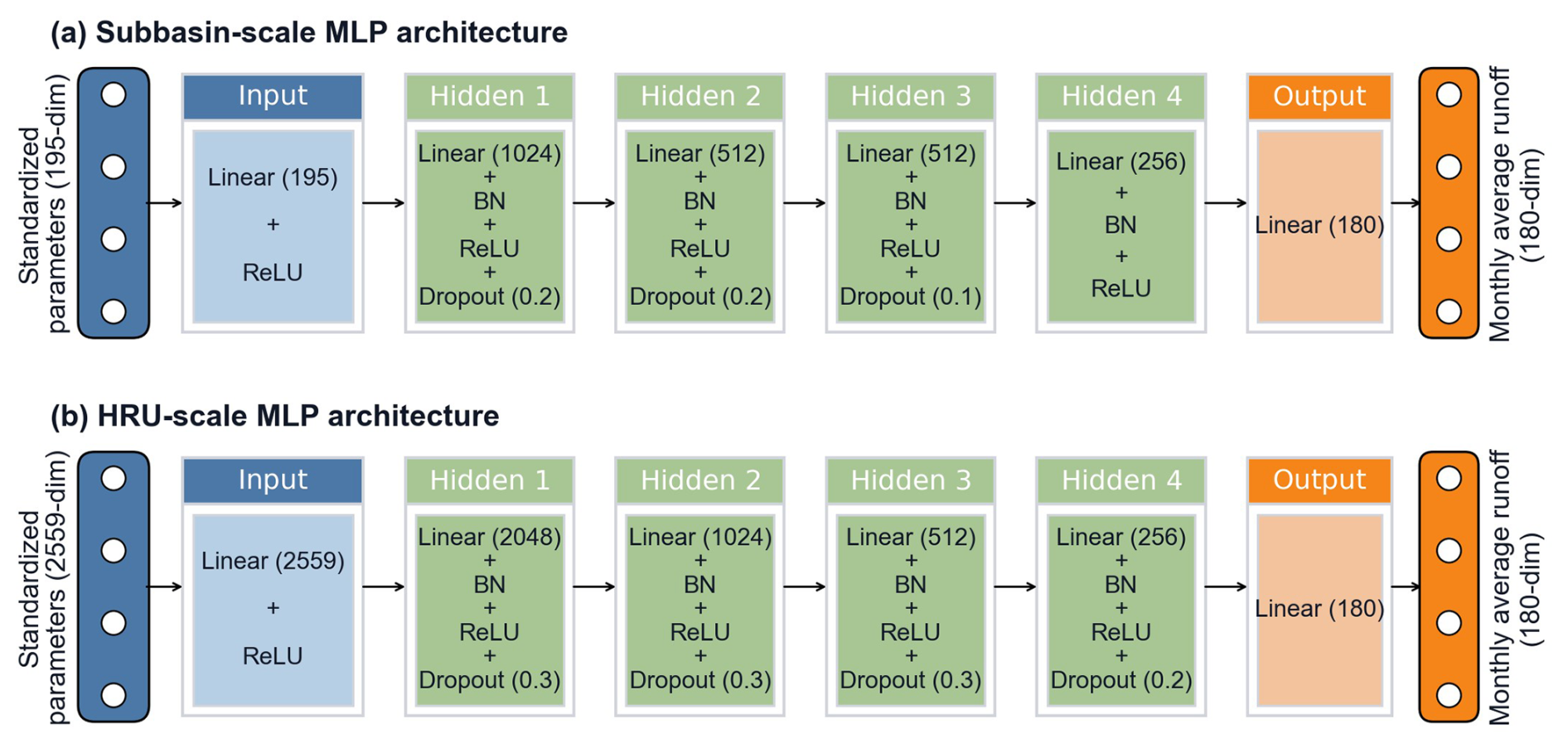
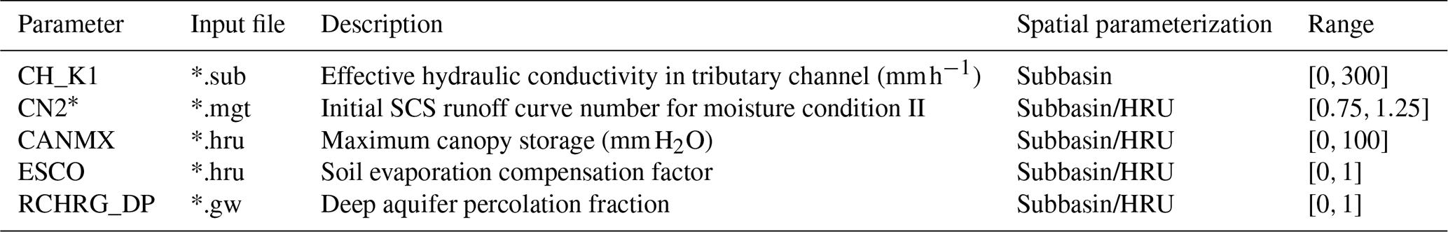
Figure 2 MLP architectures for runoff prediction at the ZJS gauge station with spatial parameterization at (a) subbasin and (b) HRU scales. Numbers in parentheses after “Linear” give layer width (number of neurons); numbers after “Dropout” give the dropout rate. ReLU activation follows every Linear layer except the final output layer.

To investigate the influence of spatial scale on parameter sensitivity, these five parameters were defined under two distinct parameterization schemes for SSA:

• Subbasin-scale parameterization. All five parameters were independently specified for each of the 39 subbasins, resulting in a total of 195 distributed parameters (39 subbasins × 5 parameters). For CH_K1, the parameter value was assigned to each subbasin and written directly to the corresponding subbasin file (*.sub). For CN2, CANMX, ESCO, and RCHRG_DP, although these parameters are stored in HRU-related files (*.mgt, *.hru, and *.gw), they were parameterized at the subbasin scale by assigning a single value (implemented either through “replace” or “factor” approach) to all corresponding HRUs within that subbasin. Consequently, spatial variability among subbasins was preserved, while variability among HRUs within a given subbasin was intentionally suppressed. This configuration provides a coarser representation of parameter heterogeneity and reflects hydrological controls aggregated at the subbasin level.

• HRU-scale parameterization. In this scheme, CH_K1 remained parameterized at the subbasin level. The other four parameters, CN2, CANMX, ESCO, and RCHRG_DP, were instead allowed to vary independently among the 630 HRUs. This resulted in a total of 2559 distributed parameters (39 subbasin-specific CH_K1 parameters + 630 × 4 HRU-specific parameters). Under this configuration, each HRU received an independently sampled value, explicitly representing within-subbasin heterogeneity associated with land use, soil properties, and slope. Compared with the subbasin-scale scheme, this parameterization substantially increases dimensionality but enables a finer characterization of local controls on runoff generation and partitioning.

The two parameterization schemes differ not only in dimensionality but also in their representation of spatial heterogeneity. In the subbasin-scale parameterization, parameter perturbations are imposed at the subbasin level, so variability mainly arises from differences among subbasins without independent HRU-level perturbations. In contrast, the HRU-scale parameterization explicitly resolves additional within-subbasin variability for CN2, CANMX, ESCO, and RCHRG_DP. This comparison enables a systematic assessment of how sensitivity patterns aggregate at the subbasin level and emerge at finer spatial resolutions, thereby elucidating the scale dependence of dominant hydrological controls.

2.5.2 Construction of deep learning surrogates

Due to the computational impracticality of applying the Sobol' method to such high-dimensional parameter spaces, particularly at the HRU scale, deep learning surrogates were constructed to efficiently emulate SWAT (Razavi et al., 2012). The task was formulated as a high-dimensional vector-to-vector regression problem, where static parameter vectors were mapped to the full 180-month runoff series at the ZJS gauge. Accordingly, fully connected MLPs were adopted because they effectively approximate complex nonlinear relationships in high-dimensional spaces. Although hydrological processes exhibit temporal dependencies, these dynamics are implicitly embedded in the SWAT-generated runoff sequences used for training. The MLP therefore learns the integrated parameter–response relationship over the entire simulation period. While sequence-based models such as LSTM networks may explicitly represent temporal dependencies (Jeong et al., 2024), the MLP achieved sufficient accuracy in this study and was selected as a parsimonious and computationally efficient surrogate model for sensitivity analysis (Yang et al., 2024; Yu et al., 2024).

To mirror the two spatial parameterization schemes, two MLP surrogates were constructed:

• Subbasin-scale MLP surrogate. This model comprises an input layer with 195 neurons corresponding to 195 distributed parameters under subbasin-scale parameterization, four hidden layers with varying neurons, and an output layer with 180 neurons representing monthly runoff over the simulation period.

• HRU-scale MLP surrogate. Designed to accommodate finer spatial details, this model contains 2559 input neurons corresponding to 2559 distributed parameters of HRU-scale parameterization and four hidden layers containing more neurons to capture the higher dimensionality of the input space. The output layer likewise contains 180 neurons representing monthly runoff.

In both models, fully connected architectures were adopted to approximate the nonlinear mapping between parameter space and runoff response. Rectified Linear Unit (ReLU) activation functions were used in all hidden layers, and dropout and batch normalization (BN) were applied to improve generalization and training stability. The detailed architectures are shown in Fig. 2. Training datasets were generated by sampling parameters from the ranges in Table 1 using the Latin Hypercube Sampling (LHS) method. For the subbasin-scale surrogate, 50 000 parameter realizations were generated, forming a 50 000 × 195 parameter matrix. For the HRU-scale surrogate, 200 000 realizations were generated, yielding a 200 000 × 2559 parameter matrix. These sample sizes balance (i) adequate coverage of the high-dimensional spaces needed for deep models and (ii) computational feasibility given the number of SWAT simulations. Preliminary experiments indicated only marginal accuracy gains beyond these sizes, confirming their adequacy.

Each sampled parameter set was evaluated using SWAT to produce the corresponding 180-month runoff series, forming paired input-output datasets for supervised learning. All simulations were executed on the High-Performance Computing (HPC) platform of Northwest A&F University, which supports parallel batch job submission, thereby greatly reducing wall-clock time. The resulting input-output datasets were randomly split into training (80 %) and testing (20 %) subsets. The MLP surrogates were implemented in PyTorch (Paszke et al., 2019) and trained using the root-mean-squared error (RMSE) loss function, optimized using the Adam algorithm with an initial learning rate of 0.001. Early stopping based on validation loss was employed to prevent overfitting. Model performance was evaluated on the testing set using RMSE, the coefficient of determination (R²), and prediction error diagnostics. Once validated, the surrogates were expected to reproduce SWAT outputs with high fidelity while drastically reducing computational cost. These trained MLPs were subsequently used in place of SWAT for SSA using the Sobol' method.

2.5.3 Spatial sensitivity analysis across subbasin and HRU scales

Using the trained surrogate models, SSA was conducted to evaluate the spatial variability of parameter sensitivity. Unlike the Morris method implemented in Sect. 2.4, which relied on the spatially lumped strategy, the SSA employed spatially disaggregated parameter definitions across 39 subbasins and 630 HRUs. Specifically, the five screened parameters were allowed to vary independently across all subbasins and HRUs, yielding 195 distributed parameters at the subbasin scale and 2559 distributed parameters at the HRU scale, as detailed earlier.

SSA was then performed using the Sobol' method at both subbasin and HRU scales:

• Subbasin-scale SSA. Two sampling matrices A and B, each comprised of 4096 realizations, were first generated using the Sobol' sequence. For each of the 195 parameters, an additional matrix C_i was constructed by replacing the ith column of A with that of B. This resulted in a total of 806 912 = 4096 × (195+2) parameter realizations.

• HRU-scale SSA. Due to the substantially higher dimensionality of the HRU-scale parameter space, each base matrix A or B contained 32 768 realizations, and corresponding C_i matrices were similarly generated. In total, this resulted in 83 918 848 = 32 768 × (2559+2) parameter realizations.

For each parameter realization at either spatial scale, the corresponding MLP surrogate generated the 180-month runoff series at the ZJS gauge station. Consistent with previous SSA studies (Herman et al., 2013b; Wu et al., 2022), sensitivity was assessed using summary performance metrics, i.e., NSE computed over the full 180-month simulation period, rather than raw streamflow values, since the objective was to evaluate the controls on overall model performance rather than on runoff alone. The generation of sampling matrices and the calculation of Sobol' sensitivity indices were performed using the SALib Python package (Herman and Usher, 2017). The Sobol' first-order S_i and total-effect S_Ti sensitivity indices were computed for the 195 distributed parameters at the subbasin scale and the 2559 distributed parameters at the HRU scale.

To ensure numerical reliability, convergence of the sensitivity estimates was assessed by progressively increasing the sample size N, together with bootstrapping using 100 replicates to estimate 95 % confidence intervals. In addition, rank stability was assessed using Spearman's rank correlation coefficient by comparing the rankings of all parameters (195 parameters at the subbasin scale and 2559 parameters at the HRU scale) obtained at each intermediate sample size N with those derived from the final reference sample size (Sarrazin et al., 2016). For visualization, subbasin-scale S_i and S_Ti values were reshaped into a 5 × 39 array, corresponding to the five parameters defined across the 39 subbasins, and mapped to their corresponding subbasins. This structure produced five geospatial maps, one for each parameter, with individual subbasins displaying the spatial distribution of parameter sensitivities. At the HRU scale, CH_K1 was mapped at the 39 subbasins, while the other four parameters (CN2, CANMX, ESCO, and RCHRG_DP) were mapped across the 630 HRUs. This yielded another five geospatial maps: one for CH_K1 at the subbasin scale and four for the remaining parameters at the HRU scale. Collectively, these spatial fields reveal the magnitude and location of influence and highlight sensitivity hotspots at each spatial scale.

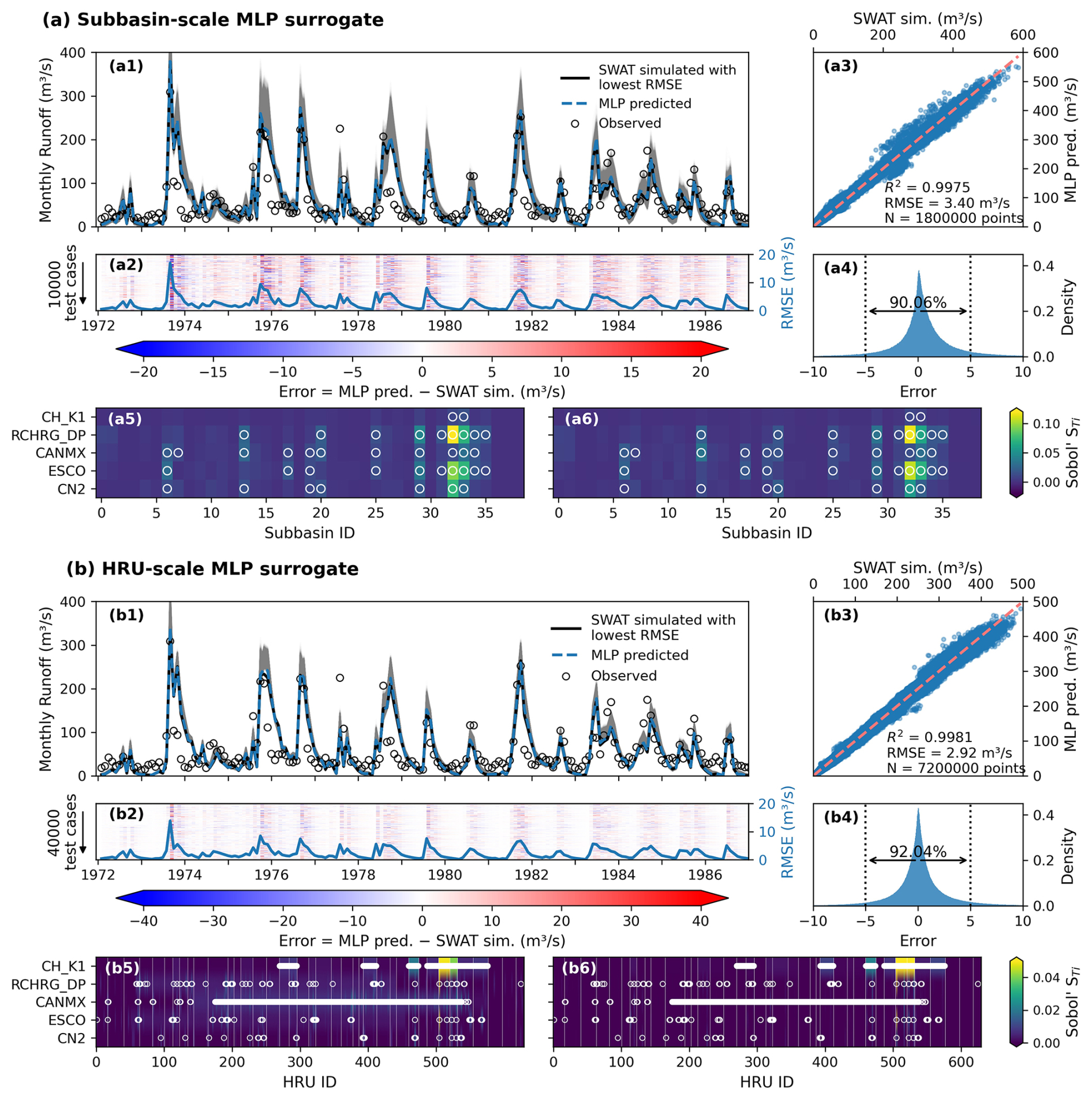
Figure 3 Performance of the trained MLP surrogates at the (a) subbasin and (b) HRU scales. Panels (a1) and (b1) compare ensemble SWAT simulations for the test cases (grey lines; 10 000 cases at the subbasin scale and 40 000 cases at the HRU scale), the specific SWAT-simulated runoff with the lowest RMSE relative to observed runoff (black lines) and the corresponding MLP-predicted runoff (blue dashed lines), as well as observed runoff (black circles) at the ZJS gauge station. Panels (a2) and (b2) show heatmaps of prediction errors across 180 months from 1972 to 1986 for all test cases; blue solid lines indicate the RMSE values calculated for each month across realizations. Panels (a3) and (b3) present scatter plots of MLP-predicted versus SWAT-simulated runoff, showing strong agreement with global R² values of 0.9975 and 0.9981, and global RMSE values of 3.40 m³ s⁻¹ and 2.92 m³ s⁻¹ , respectively. Panels (a4) and (b4) show the error density, which further indicates that 90.06 % and 92.04 % of monthly prediction errors fell within ± 5 m³ s⁻¹ for the subbasin- and HRU-scale MLP surrogates, respectively, confirming high predictive fidelity. Panels (a5) and (b5) show the S_Ti using SWAT model outputs with small parameter realizations N=64 for subbasin-scale SSA and HRU-scale SSA, respectively, and Panels (a6) and (b6) show the S_Ti using outputs from the corresponding MLP surrogates with the same parameter realizations. White circles denote the top 20 % S_Ti values.

3 Results

3.1 Performance of deep learning surrogates

Figure 3 evaluates the performance of the MLP surrogates in terms of both predictive accuracy and their ability to preserve sensitivity structures. The subbasin- and HRU-scale surrogates were tested on 10 000 and 40 000 independent realizations, respectively, each producing 180-month runoff series at the ZJS gauge station. Overall, both surrogates reproduced SWAT-simulated runoff with high fidelity (Fig. 3a1 and b1). The global coefficient of determination R² reached 0.9975 and 0.9981 for the subbasin- and HRU-scale surrogates, respectively, with corresponding RMSE values of 3.40 and 2.92 m³ s⁻¹ (Fig. 3a3 and b3). Error distributions were centered near zero, with 90.06 % and 92.04 % of monthly prediction errors falling within ± 5 m³ s⁻¹ (Fig. 3a4 and b4). The temporal structure of prediction errors illustrated in Fig. 3a2 and b2 shows larger deviations during high-flow periods, reflecting the challenges of emulating nonlinear and threshold-driven hydrological processes such as saturation-excess runoff and channel routing. These discrepancies may be partly attributable to the limited representation of extreme events in the training dataset. Nevertheless, such limitations do not compromise the primary objective of this study, as the surrogate models are intended to emulate SWAT for SA rather than to replace process-based simulations of extreme hydrological events.

Beyond predictive accuracy, the ability of the surrogates to preserve sensitivity structures was explicitly evaluated using a small number of parameter realizations (N=64), necessitated by the substantial computational cost of running the original SWAT model. At both the subbasin and HRU scales, SSA was conducted using the same parameter samples for both the original SWAT model and the corresponding MLP surrogate model. This produced two sets of sensitivity indices, allowing direct comparison between the SWAT-based and MLP-based sensitivity results. Figure 3a5–a6 and b5–b6 compare the S_Ti values computed from SWAT outputs with those derived from the corresponding MLP surrogates at the subbasin and HRU scales, respectively. The results show strong agreement in both the magnitude and distribution of dominant sensitivity signals, with only minor discrepancies in numerical values. Notably, the ranking and identification of the top 20 % most influential parameters are identical, as highlighted by the white circles. These findings confirm that the surrogate models effectively preserve the relative importance and ranking of parameters, thereby providing confidence that the subsequent surrogate-based SSA reliably captures the key controls of the original SWAT model.

From a computational standpoint, the efficiency gains through the MLP surrogates were transformative. A single SWAT simulation takes ∼ 10 s of CPU time on a 2.2 GHz Intel^® Core™ i7-14650HX laptop. In contrast, the trained subbasin-scale MLP surrogate completed 806 912 evaluations in ∼ 2 s, corresponding to ∼ 2.5 × 10⁻⁶ s per evaluation, and the HRU-scale MLP surrogate completed 83 918 848 evaluations in ∼ 475 s, corresponding to ∼ 5.7 × 10⁻⁶ s per evaluation. These correspond to speed-ups ∼ 4.0 × 10⁶ and ∼ 1.8 × 10⁶, respectively, i.e., efficiency gains exceeding six orders of magnitude relative to the original SWAT model. Such acceleration renders SA at multiple spatial and temporal scales computationally tractable. Additionally, this remarkable efficiency enables rapid parameter screening and supports downstream applications such as real-time forecasting, model-data fusion, and optimization-based decision support within distributed hydrologic modelling frameworks.

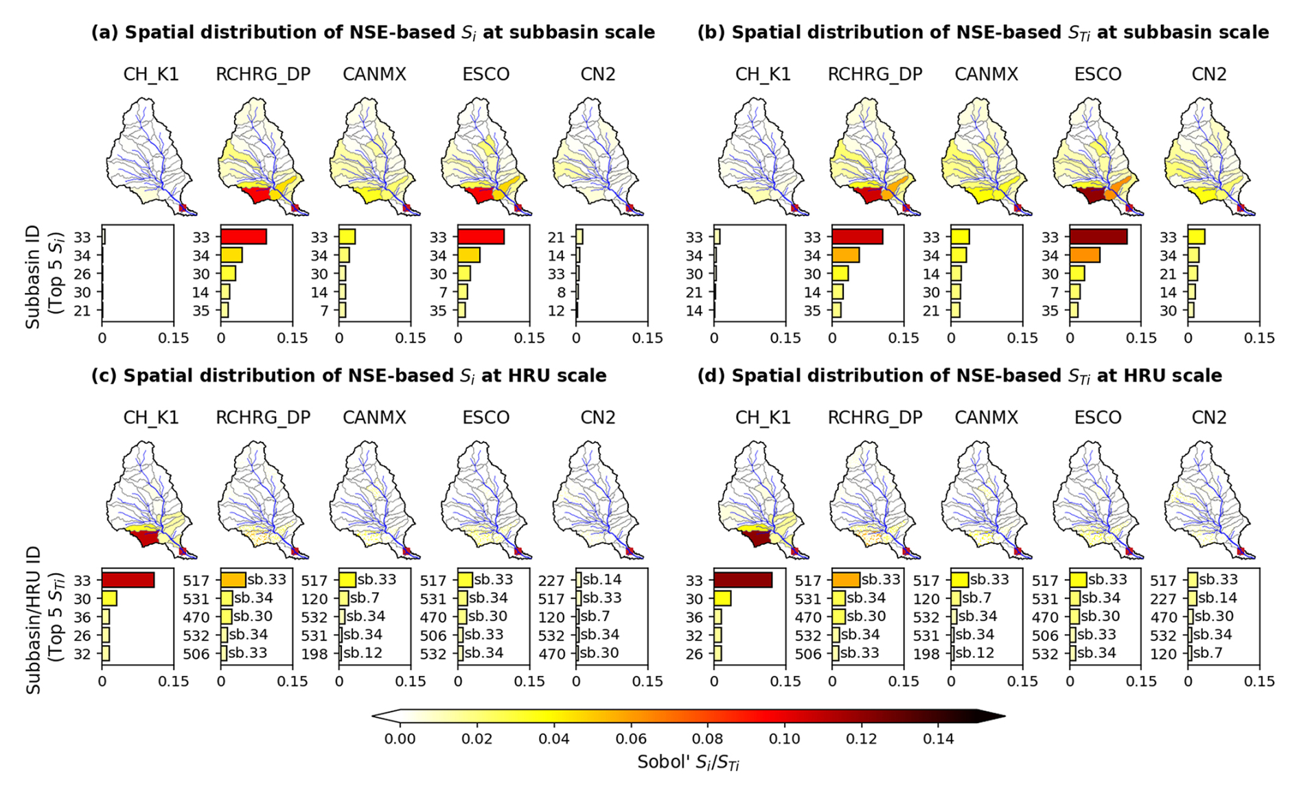
Figure 4 Spatial distribution of the total-effect sensitivity index S_Ti to NSE evaluated at ZJS gauge station by (a) subbasin-scale SSA and (b) HRU-scale SSA. Bar plots below each map show the top ten subbasins/HRUs ranked by S_Ti. For the HRU-scale plots, the text to the right of each bar indicates the parent subbasin (e.g., HRU 517 belongs to subbasin 33, denoted as sb. 33).

3.2 Spatial distribution of parameter sensitivities at subbasin and HRU scales

Figure 4 maps the spatial distribution of S_i and S_Ti for the five screened parameters, using the NSE computed over the 180-month simulation period as the response metric in both subbasin- and HRU-scale SSA. The accompanying bar plots highlight the five most sensitive subbasins or HRUs for each parameter. Convergence is evidenced by the progressive narrowing of the 95 % bootstrap confidence intervals of the sensitivity estimates and the stabilization of parameter rankings (Fig. S5 in the Supplement). Moreover, convergence analysis shows that S_Ti exhibits more stable convergence behaviour than S_i. Parameter rankings based on S_Ti became effectively identical beyond the sample size of N=512 for the subbasin-scale SSA and N=2048 for the HRU-scale SSA. These results indicate that the identification of dominant parameters is robust with respect to the final reference sample sizes of N=4096 and N=32 768, respectively.

Several key observations can be drawn from Fig. 4. First, the spatial patterns of S_i and S_Ti are broadly consistent at both the subbasin and HRU scales. The rankings of the most sensitive subbasins and HRUs are similar between the two indices for each parameter, indicating that the dominant controls are robust to the choice of sensitivity indices. Considering S_Ti accounts for both the main effects of individual parameters and their interactions (Yang et al., 2024), it provides a more comprehensive measure of parameter influence. Therefore, the following analyses focus primarily on S_Ti.

Second, sensitivity exhibits pronounced spatial heterogeneity. At the subbasin scale (Fig. 4a and 4b), high sensitivity values are unevenly distributed and predominantly concentrated near the ZJS gauge station (outlet of subbasin 36; marked as a red square). Subbasins 33 and 34 consistently emerge as sensitivity hotspots across all parameters, highlighting their dominant role in controlling runoff variability. This pattern reflects the strong influence of gauge-proximal regions, where parameter perturbations are efficiently transmitted to the observed hydrograph, consistent with previous findings (e.g., Tang et al., 2007). Additional subbasins, such as 14, 21, and 30, and occasionally upstream subbasins, such as 7 and 8, also appear among the most sensitive units for specific parameters, suggesting localized process dominance. In contrast, downstream subbasins (37–39), located below the gauge, exhibit near-zero sensitivity, confirming their negligible influence on the evaluated discharge. At the HRU scale (Fig. 4c and 4d), sensitivity remains highly uneven across both subbasins and HRUs. Large portions of the basin, particularly upstream regions, show near-zero S_Ti values, partly reflecting the increased parameter dimensionality at finer spatial resolution.

Third, sensitivity patterns become more spatially localized at the HRU scale. While the most sensitive HRUs remain concentrated within subbasins 33 and 34, substantial heterogeneity is observed within individual subbasins. For example, HRU 517 (in subbasin 33) consistently ranks among the most sensitive units across multiple parameters, whereas neighbouring HRUs exhibit negligible sensitivity. This intra-subbasin variability highlights the role of local heterogeneity in soil properties, topography, and land cover, which is not captured at the aggregated subbasin scale.

Fourth, a scale-dependent redistribution of parameter importance and partial decoupling between subbasin- and HRU-scale sensitivities are observed. Certain HRUs exhibit high sensitivity even when their parent subbasins are not identified as hotspots at the subbasin scale (e.g., HRU 198 in subbasin 12 for CANMX), indicating that spatial aggregation can obscure localized controls. Additionally, the relative importance of CH_K1 increases at finer spatial resolution. This behaviour reflects a scale-interaction mechanism: as the other four parameters (CN2, ESCO, CANMX, and RCHRG_DP) are disaggregated to the HRU level, the routing effect governed by CH_K1 integrates numerous heterogeneous local responses, thereby increasing its contribution to overall model performance. This finding is consistent with previous studies (e.g., Acero Triana et al., 2025).

Overall, these results reveal clear scale-dependent sensitivity patterns, underscoring the importance of accounting for spatial heterogeneity when interpreting model behaviour and designing subsequent model applications.

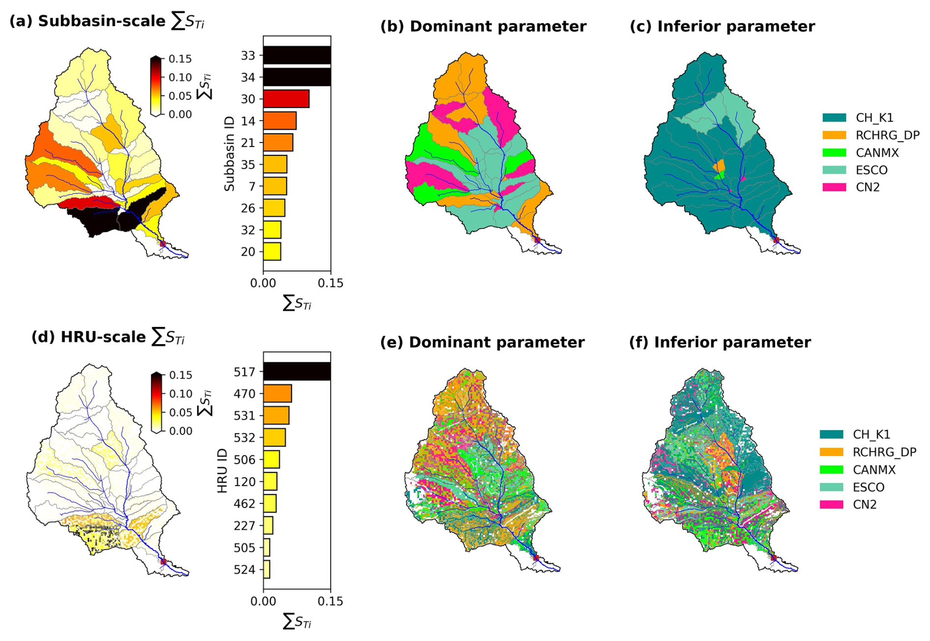
Figure 5 Spatial distribution of sensitivity patterns across subbasin and HRU scales. Panels (a) and (d) show the sum of S_Ti of the five screened parameters, ΣS_Ti, at the subbasin and HRU scales, respectively. Panels (b) and (e) present the spatial distribution of the dominant parameter. Panels (c) and (f) present the spatial distribution of the inferior parameter.

3.3 Identification of sensitivity hotspots and parameter hierarchies

To further elucidate the scale effects on this heterogeneity, we computed the sum of the total-effect sensitivity indices S_Ti of the five screened parameters, denoted as ΣS_Ti, for each spatial unit (Fig. 5a and d). Specifically, the five S_Ti maps derived from subbasin- and HRU-scale SSA (Fig. 4b and d) were overlaid and summed to derive the spatial distributions of ΣS_Ti, respectively. Because CH_K1 is defined only at the subbasin level, its sensitivity values were uniformly distributed to the HRUs within each corresponding subbasin when calculating ΣS_Ti at the HRU scale. Considering S_Ti quantifies the total contribution of parameter i to output variance, ΣS_Ti provides a compact measure of a unit's overall responsiveness to model perturbations, namely, its ability to transmit parameter uncertainty into variations in NSE at the ZJS gauge station. Consequently, larger ΣS_Ti values delineate spatial sensitivity hotspots.

Figure 5a and d show that the overall spatial organization of sensitivity is consistent across scales, while increasing spatial resolution sharpens its localization. At the subbasin scale, subbasins 33 and 34 (and to a lesser extent subbasin 30) consistently emerge as dominant hotspots. At the HRU scale, these hotspots are further resolved into a limited number of highly sensitive HRUs nested within these subbasins, such as HRU 517 (subbasin 33), HRUs 531 and 532 (subbasin 34), and HRU 470 (subbasin 30). This indicates that increasing spatial resolution refines the localization of sensitivity rather than altering the identification of key regions. The observed refinement may reflect underlying heterogeneity in land cover, soil properties, and topography, whereby only a subset of HRUs within each subbasin contributes disproportionately to the total sensitivity.

Figure 5b and e further characterize the spatial hierarchy of parameter influence by identifying, for each spatial unit, the dominant parameter (defined as the parameter with the maximum S_Ti), while Fig. 5c and f identify the inferior parameter (defined as the parameter with the minimum S_Ti). At the subbasin scale, Fig. 5b indicates that sensitivity hotspots are governed by different hydrological controls. While subbasins 33 and 34 are dominated by ESCO, subbasin 30 is primarily controlled by RCHRG_DP. This distinction demonstrates that hotspot magnitude and dominant mechanism are related but not interchangeable, as highly sensitive subbasins may respond to different hydrological processes. As for the inferior parameter map, Fig. 5c exhibits a clearer pattern: CH_K1 is consistently identified as the least influential parameter across nearly all subbasins. This reflects the limited impact of channel hydraulic conductivity on the NSE-based outlet response compared to parameters controlling runoff generation, evapotranspiration, and recharge partitioning. Perturbations in channel routing processes are progressively damped through downstream aggregation, resulting in negligible contributions to hydrograph variance. At the HRU scale, the dominant parameter map (Fig. 5e) becomes markedly fragmented, indicating increased local process heterogeneity. Although the subbasin-scale hotspot pattern persists, it decomposes into a mosaic of HRUs governed by different parameters. Within subbasins 33 and 34, some HRUs remain dominated by CH_K1, while others are controlled by RCHRG_DP, ESCO, or CN2. This finer-scale differentiation suggests that dominant mechanisms depend strongly on local combinations of soil properties, land use, and topography. Thus, HRU-scale analysis provides a more realistic representation of distributed hydrological processes by revealing multiple coexisting controls within a single subbasin.

The inferior-parameter map at the HRU scale (Fig. 5f) is also highly localized. Notably, many HRUs near the basin outlet are characterized by CANMX as the least influential parameter. This indicates that canopy interception has a comparatively minor impact on the NSE-based outlet response relative to processes governing runoff partitioning, groundwater recharge, evapotranspiration, and routing. Because outlet discharge integrates upstream hydrological signals, the incremental effect of local interception storage becomes attenuated, rendering CANMX relatively insignificant in downstream HRUs. More broadly, the HRU-scale results reveal that inferior processes vary spatially: while CH_K1 frequently appears least influential in upstream regions at the subbasin scale, the HRU-scale analysis shows that inferior status can shift locally among CH_K1, CANMX, ESCO, and CN2. This demonstrates that spatial aggregation masks not only local hotspots but also local process irrelevance. Consequently, the inferior parameter map complements the dominant-parameter map by identifying processes that can be deprioritized locally.

4 Discussion

4.1 Effects of performance metrics on sensitivity patterns

Although the primary sensitivity analysis in this study was conducted using the NSE, it is necessary to examine whether the identified sensitivity patterns are robust with respect to the choice of performance metrics. Because NSE primarily reflects variance-based agreement and is particularly sensitive to peak flow dynamics and temporal variability, two widely used complementary metrics, PBIAS and KGE, were introduced (Clark et al., 2021). These metrics provide distinct yet complementary perspectives on hydrological model performance: PBIAS quantifies systematic bias in the water balance, whereas KGE offers a balanced evaluation by integrating correlation, bias, and variability (Acero Triana et al., 2025; Tuo et al., 2018).

The Morris screening results based on PBIAS and KGE reveal differences in parameter identification compared with those obtained using NSE. PBIAS identifies CANMX, CN2, ESCO, RCHRG_DP, and SOL_BD as the five most influential parameters (Fig. S6 in the Supplement), whereas KGE highlights ALPHA_BF, CN2, ALPHA_BNK, CANMX, and ESCO (Fig. S7 in the Supplement). Despite these differences, a notable consistency emerges: all parameters identified as sensitive under NSE remain within the top-ranked subset identified by PBIAS and KGE (i.e., within the top 15 of 33 candidates). This indicates that, although relative rankings vary across metrics, the core set of influential parameters remains largely unchanged. In other words, the sensitivity structure of the system is robust, and the influence of performance metric selection is primarily reflected in the magnitude and ordering of sensitivities rather than in the identification of fundamentally different controls.

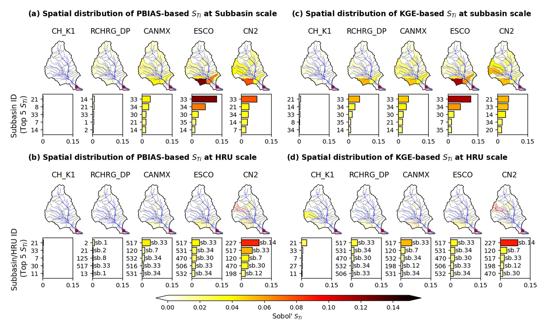
Figure 6 Spatial distribution of the total-effect sensitivity index S_Ti at the subbasin and HRU scales using different performance metrics. Panels (a) and (b) show results based on PBIAS, and panels (c) and (d) show results based on KGE.

To ensure direct comparability of spatial sensitivity patterns across performance metrics, the five NSE-screened parameters were retained for SSA, with PBIAS and KGE replacing NSE as response metrics. This offers two advantages: it enables direct spatial comparison of sensitivity patterns across metrics and eliminates the need to retrain the MLP surrogates. Specifically, the trained subbasin- and HRU-scale surrogates were used to predict runoff at ZJS station, from which PBIAS and KGE were computed instead of NSE. Figure 6 presents the spatial distributions of S_Ti based on PBIAS and KGE at both subbasin and HRU scales. At the subbasin scale, although slight differences in sensitivity magnitude and parameter ranking are observed, the overall spatial patterns are highly consistent with those obtained using NSE (Fig. 4). In particular, subbasins 33 and 34 consistently exhibit the highest sensitivity, while sensitivity decreases progressively toward upstream regions, and downstream subbasins still show negligible influence. These results confirm that the locations of sensitivity hotspots are primarily governed by hydrological connectivity and proximity to the gauge station, and that these spatial patterns are largely independent of the performance metric. At the HRU scale, the sensitivity patterns derived from PBIAS and KGE are also broadly consistent with those based on NSE. Sensitivity remains highly localized, with only a limited number of HRUs exerting significant influence, while the majority of units contribute negligibly. This suggests that parameter sensitivity at the HRU scale is dominated by local hydrological conditions rather than by large-scale aggregation effects, and that this characteristic is robust across different performance metrics.

A notable exception is observed for the parameter CH_K1. Under NSE, CH_K1 exhibits much higher sensitivity at the HRU scale, whereas its influence becomes substantially weaker when evaluated using PBIAS and KGE. This discrepancy cannot be fully explained by spatial aggregation, as CH_K1 is consistently defined at the subbasin scale in all analyses. Instead, the difference may arise from the distinct aspects of model behaviour emphasized by each performance metric. CH_K1 primarily controls flow routing processes, affecting the timing and attenuation of streamflow. NSE is highly sensitive to such changes because it strongly penalizes discrepancies in peak flow and temporal variability. In contrast, PBIAS, which measures only cumulative bias, is largely insensitive to timing errors. Similarly, although KGE incorporates a correlation component, its composite structure reduces the relative influence of timing-related effects compared to NSE. As a result, the sensitivity of CH_K1 is significantly diminished under PBIAS and KGE.

4.2 Effects of parameter distributions on sensitivity patterns

As mentioned earlier, the sensitivity patterns presented in Sect. 3 were based on parameter ranges derived from previous studies and the SWAT theoretical documentation. These ranges are hereafter referred to as the prior distributions. Considering the assumed parameter distributions may affect the estimation of the sensitivity indices, an additional SSA was conducted using NSE-constrained posterior parameter distributions, in which the original prior distributions were updated by retaining only parameter realizations associated with acceptable model performance (Wu et al., 2022). Specifically, NSE values were calculated for 50 000 SWAT simulations generated for the subbasin-scale parameterization and 200 000 simulations for the HRU-scale parameterization (Fig. S8 in the Supplement). Two performance thresholds were considered: NSE > 0.1 and NSE > 0.3. For each threshold, parameter realizations satisfying the criterion were extracted and treated as behavioural ensembles. Figure S9 in the Supplement compares the prior and posterior distributions for the four parameters with the largest Kolmogorov–Smirnov (KS) statistics, together with histograms of KS values across all distributed parameters. Under the weaker constraint (NSE > 0.1), posterior distributions show only minor deviations from the priors, especially at the HRU scale. Under the stricter constraint (NSE > 0.3), noticeable departures occur for a limited subset of influential parameters, indicating stronger performance constraints. Nevertheless, even under this stricter constraint, over 92 % of parameters at the subbasin scale and 99 % at the HRU scale exhibit KS values below 0.1, indicating minimal deviations between prior and posterior distributions.

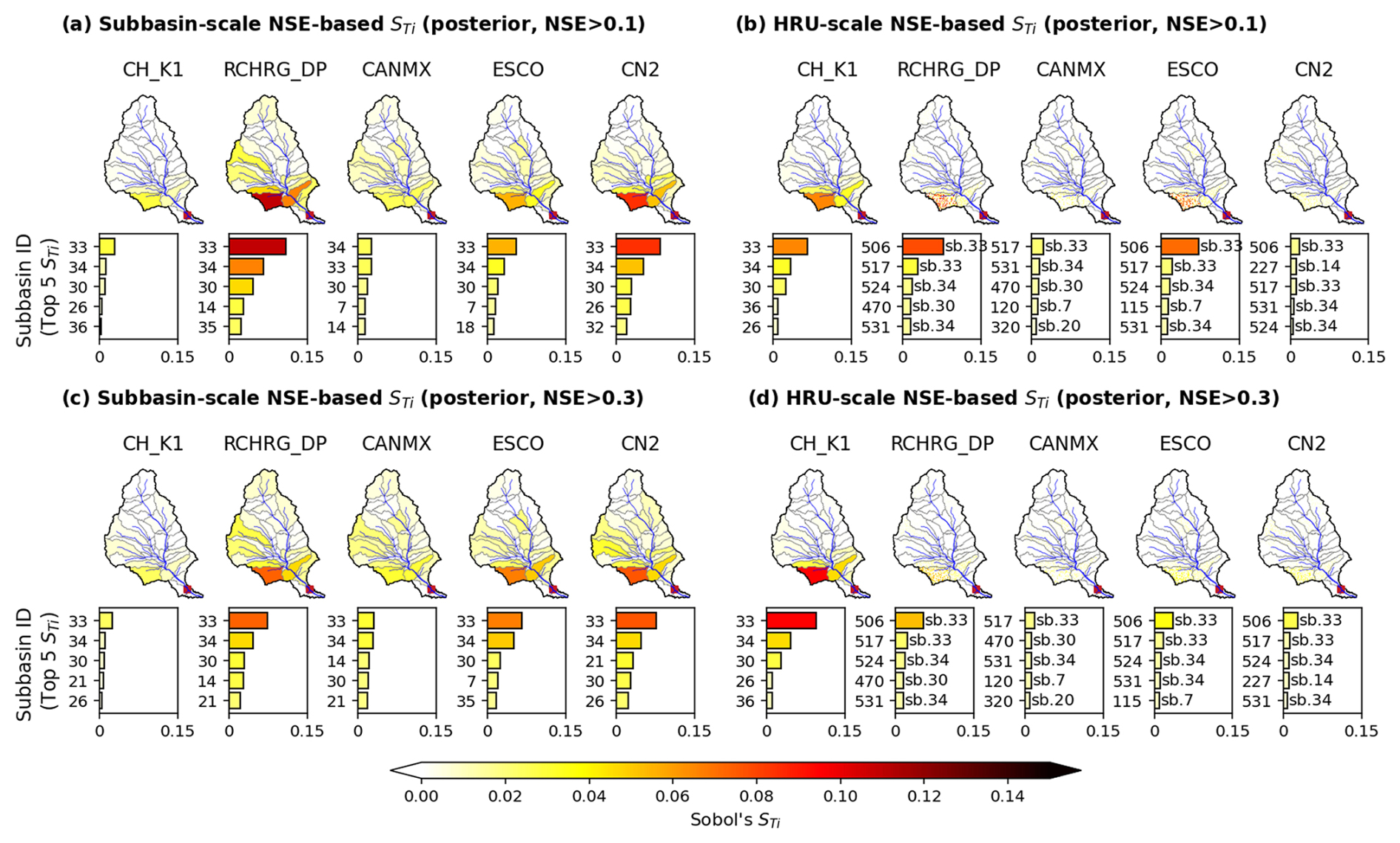
Figure 7 Spatial distribution of the total-effect sensitivity index S_Ti at the subbasin and HRU scales using posterior parameter distributions constrained by different NSE thresholds. Panels (a) and (b) show results constrained by NSE > 0.1, and panels (c) and (d) show results constrained by NSE > 0.3.

Based on these NSE-constrained posterior distributions, the MLP-assisted SSA was repeated at both the subbasin and HRU scales. In practice, the posterior distributions were represented empirically by the behavioural parameter samples. New sampling matrices, A, B and C_i, were generated by resampling from these empirical posterior marginals prior to surrogate-based evaluation. The trained MLP surrogate models were then used to generate the corresponding model outputs. Note the MLP surrogate models were not re-trained for the posterior-based SSA because the posterior parameter samples remained within the same parameter bounds used during surrogate training, although their probability distributions changed from uniform prior distributions to empirical posterior distributions. The resulting sensitivity maps are presented in Fig. 7. Compared with the prior-based results shown in Fig. 4b and d, the overall spatial sensitivity patterns remain remarkably consistent. At both scales, the principal sensitivity hotspots are preserved, and the same key regions continue to exert dominant control on the runoff at the ZJS gauge station. In particular, the gauge-proximal hotspot remains the primary area of high sensitivity, and the most influential HRUs remain concentrated within the same subbasins identified under the prior analysis. The primary differences arise not in the spatial distribution of hotspots, but in the magnitude of the total-effect indices S_Ti and in the relative prominence of a few locally dominant parameters. This behaviour is consistent with the KS analysis. Because the vast majority of distributed parameters exhibit only minor deviations between prior and posterior distributions, the global sensitivity structure remains largely unchanged. Nevertheless, a limited subset of parameters shows stronger prior–posterior differences, which are sufficient to alter the precise values of the Sobol' indices. In other words, constraining the parameter space modifies how variance is partitioned among influential parameters without fundamentally altering where sensitivity is concentrated.

Overall, these results demonstrate that the inferred spatial sensitivity patterns are robust to moderate posterior conditioning. Restricting the parameter space to behaviourally acceptable regions affects the absolute magnitude of sensitivity indices more than their spatial organization. This finding confirms that the hotspot patterns identified in the prior-based analysis are not merely artifacts of broad literature-derived parameter ranges, but instead reflect persistent structural characteristics of the model and watershed response. At the same time, the posterior-based analysis indicates that stricter behavioural constraints can subtly redistribute sensitivity magnitudes, underscoring the importance of incorporating parameter realism when interpreting quantitative sensitivity results.

4.3 Effects of including an upper stream gauge on sensitivity patterns

The preceding analyses were conducted using the ZJS gauge station, located near the watershed outlet, which integrates the cumulative hydrological response of the entire basin. While such an outlet-based evaluation provides a comprehensive assessment of basin-scale dynamics, it may obscure spatial variability in upstream processes. To investigate the influence of observation location on sensitivity patterns, an additional gauge, the YJP station, situated in the upper basin (Fig. 1c), was incorporated into the analysis.

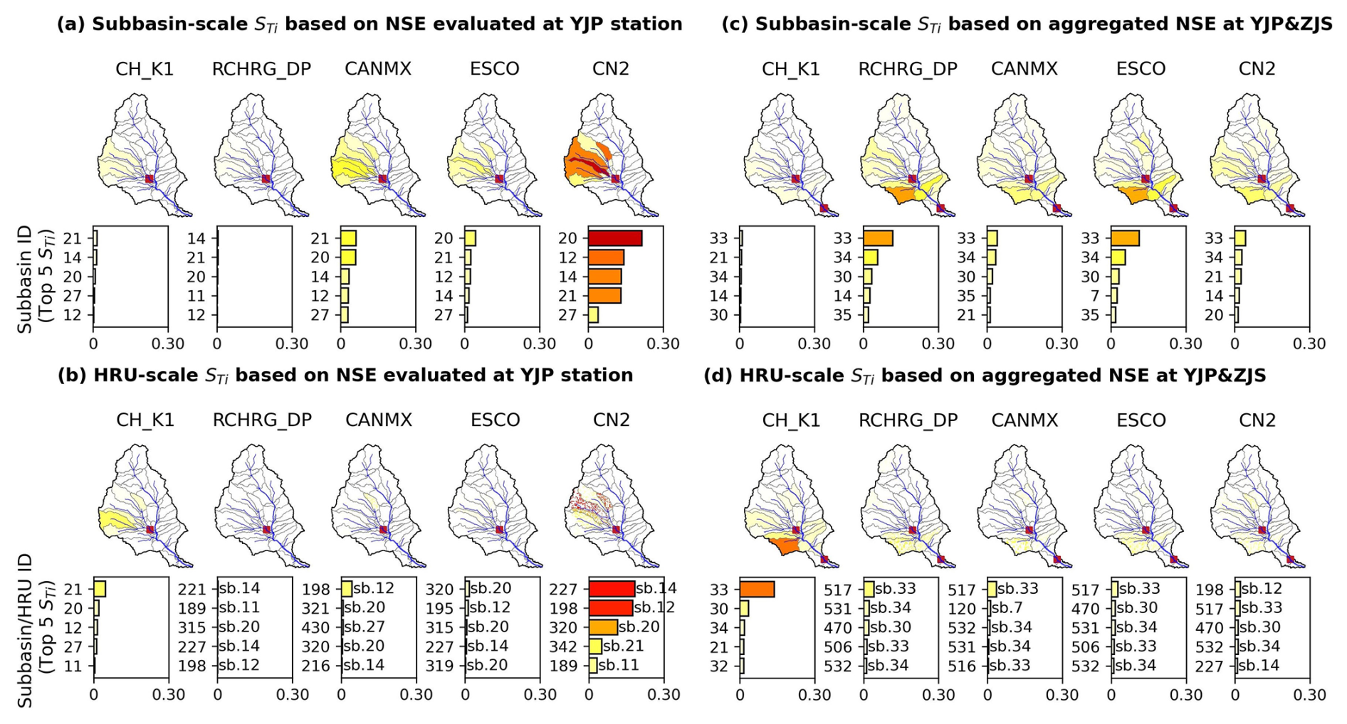
Figure 8 Spatial distribution of Sobol' total-effect sensitivity index S_Ti at the subbasin and HRU scales using different observation configurations. Panels (a) and (b) show results based on NSE evaluated at the YJP gauge station, and panels (c) and (d) show results based on aggregated NSE evaluated across YJP and ZJS stations.

The Morris screening analysis based on NSE evaluated at the YJP station identified the same five most influential parameters as those obtained from the ZJS-based analysis, indicating that parameter influence is largely consistent across gauges (Fig. S10 in the Supplement). However, both the Morris indices μ^∗ and σ^∗ at YJP are systematically smaller than those at ZJS. This reduction can be attributed to the smaller contributing area of the YJP station, where upstream processes are less spatially aggregated and thus exhibit reduced overall variance. Subsequently, subbasin- and HRU-scale surrogate models were developed for the YJP station using the same MLP architecture, with RMSE as the training objective (model performance shown in Fig. S11 in the Supplement). The resulting spatial distributions of total-effect sensitivity indices S_Ti are presented in Fig. 8.

At both subbasin and HRU scales, the spatial patterns of S_Ti at the YJP station exhibit strong similarities to those obtained using ZJS (Fig. 4), with sensitivity concentrated near the observation location and becoming increasingly localized at finer spatial resolution. A notable feature is that parameters located downstream of the YJP station exhibit near-zero sensitivity, confirming that downstream processes do not influence upstream observations. This result reinforces the causal structure of the hydrological system and demonstrates that sensitivity is constrained by flow direction and information propagation pathways. Another important observation is that the magnitude of S_Ti values at YJP is generally higher than those obtained using ZJS. This can be explained by the reduction in the effective parameter space: since downstream parameters have negligible influence on YJP, the total variance contribution is redistributed among a smaller set of influential parameters, leading to higher individual S_Ti values. In other words, the same total variance is partitioned among fewer effective parameters, resulting in an apparent increase in sensitivity magnitude.

To further explore the effect of multiple observation constraints, we constructed an aggregated NSE across the YJP and ZJS stations:

$$\begin{array}{}\text{(5)}& {\text{NSE}}_{\text{agg}}=\mathrm{1}-{\displaystyle \frac{\begin{array}{c}{\sum }_{i=\mathrm{1}}^n{\left(Q_{\mathrm{o},i}^{\text{ZJS}}-Q_{\mathrm{s},i}^{\text{ZJS}}\right)}^{\mathrm{2}}\\ +{\sum }_{i=\mathrm{1}}^n{\left(Q_{\mathrm{o},i}^{\text{YJP}}-Q_{\mathrm{s},i}^{\text{YJP}}\right)}^{\mathrm{2}}\end{array}}{\begin{array}{c}{\sum }_{i=\mathrm{1}}^n{\left(Q_{\mathrm{o},i}^{\text{ZJS}}-\stackrel{\mathrm{‾}}{Q_{\mathrm{o}}^{\text{ZJS}}}\right)}^{\mathrm{2}}\\ +{\sum }_{i=\mathrm{1}}^n{\left(Q_{\mathrm{o},i}^{\text{YJP}}-\stackrel{\mathrm{‾}}{Q_{\mathrm{o}}^{\text{YJP}}}\right)}^{\mathrm{2}}\end{array}}},\end{array}$$

where n=180 is the number of months in the evaluation period; Q_s,i and Q_o,i are the SWAT simulated and observed runoff at month i, respectively; $\stackrel{\mathrm{‾}}{Q_{\mathrm{o}}}$ represents the mean observed runoff over the evaluation period. This formulation extends the NSE to a multi-site context by aggregating squared errors and variances across stations, thereby preserving the variance-weighted contributions of each site.

The Morris analysis based on this aggregated NSE again identifies the same five dominant parameters (Fig. S12 in the Supplement). However, the sensitivity magnitudes exhibit an intermediate behaviour: they are larger than those obtained using the upstream YJP station alone but smaller than those derived from the downstream ZJS station. This pattern arises from the definition of NSE, as the aggregated objective combines the error structures of both stations, increasing both the numerator and denominator. Consequently, the relative contributions of individual parameters are moderated, resulting in intermediate sensitivity magnitudes. Surrogate models were then trained using the aggregated RMSE of both stations, followed by Sobol' SSA at the subbasin and HRU scales.

Figure 8c and d show that the spatial distribution of S_Ti under the aggregated NSE remains largely consistent with the patterns obtained using the ZJS station alone (Fig. 4b and d). In particular, the most sensitive subbasins and HRUs are nearly identical to those identified in the ZJS-based analysis. This indicates that the downstream gauge exerts a dominant control on the sensitivity structure, even when additional upstream information is incorporated. The limited influence of the YJP station in the aggregated analysis can be explained by both hydrological and statistical factors. Hydrologically, the ZJS station integrates the full upstream domain, whereas YJP only reflects a subset of the basin. Statistically, the aggregated NSE is dominated by the station with larger variance and stronger signal integration, which in this case is the downstream ZJS station. Consequently, parameter perturbations that significantly affect ZJS tend to dominate the combined objective function, while those primarily affecting YJP have a comparatively smaller impact. This result highlights an important implication: in multi-site calibration or sensitivity analysis, downstream gauges may exert disproportionate influence due to their integrative nature. As a result, simply combining multiple stations into a single objective function does not guarantee balanced sensitivity representation across the basin.

4.4 Effects of screened parameters on sensitivity patterns

The present study employs a two-step sensitivity analysis approach where the Morris method is used for parameter screening prior to SSA using the Sobol' method. While this approach substantially improves computational efficiency, the resulting sensitivity patterns may depend on the subset of parameters retained after screening. To evaluate the robustness of this framework, the SSA was extended to include four additional parameters, i.e., SOL_AWC, SOL_BD, GWQMN, and GW_DELAY, which exhibit lower Morris μ^∗ values than the original five parameters but remain more influential than the remaining candidates (Fig. S4). This extension resulted in a total of nine screened parameters and, consequently, the number of distributed parameters increased to 351 at the subbasin scale (39 subbasins × 9 parameters) and 5079 at the HRU scale (39 subbasin-specific CH_K1 parameters + 630 × 8 HRU-specific parameters).

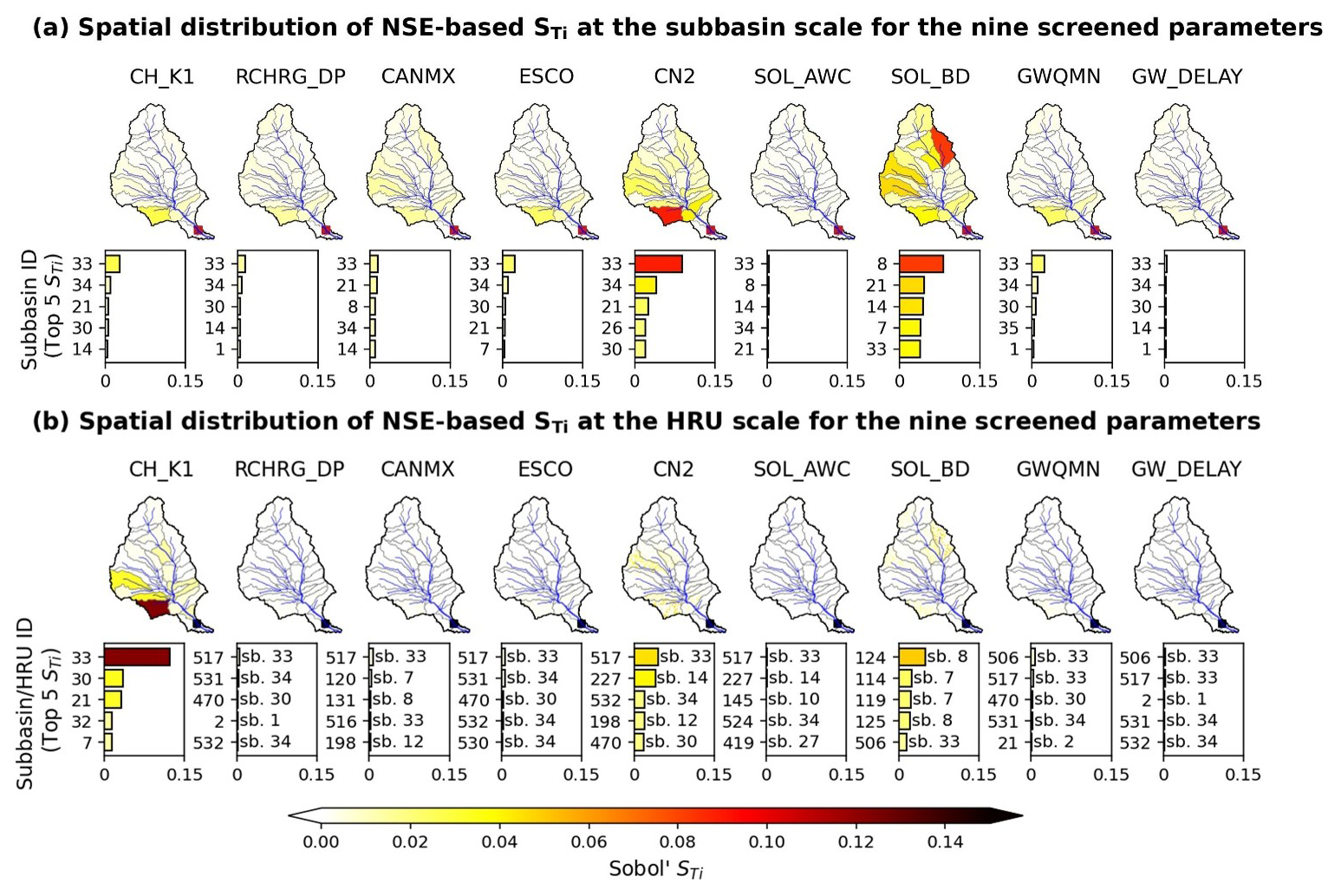
Figure 9 Spatial distribution of the total-effect sensitivity index S_Ti for the nine screened parameters at (a) the subbasin and (b) HRU scales.

To ensure computational feasibility, the MLP-assisted SSA framework was again employed. A total of 100 000 SWAT simulations were conducted to construct the surrogate model for the subbasin-scale parameterization, and 200 000 simulations were performed for the HRU-scale parameterization. Although the predictive performance of the surrogate models slightly decreased due to the increased dimensionality, their accuracy remained satisfactory for reliable sensitivity estimation (Fig. S13 in the Supplement). Using these trained surrogate models, the total-effect sensitivity indices S_Ti were computed, and their spatial distributions for the nine screened parameters are presented in Fig. 9.

The inclusion of additional parameters leads to a redistribution of variance contributions but does not fundamentally alter the spatial sensitivity patterns. At both subbasin and HRU scales, sensitivity hotspots remain concentrated near the basin outlet and within key subbasins, particularly subbasins 33 and 34. The dominant parameters identified in the original five-parameter analysis remain influential, demonstrating that the primary controls on model performance are robust to the inclusion of additional parameters. These results confirm that the two-step sensitivity analysis framework effectively captures the principal sources of uncertainty while maintaining computational efficiency.

Notably, the inclusion of soil-related parameters provides additional insights into process representation. Among the newly introduced parameters, SOL_BD exhibits localized but appreciable sensitivity, particularly in regions characterized by distinct soil properties. This behaviour highlights the importance of spatial heterogeneity in distributed hydrological modelling. The apparent discrepancy between Morris screening and Sobol' sensitivity analysis can be attributed to differences in parameter perturbation strategies and spatial representation. In the Morris analysis, parameters such as RCHRG_DP and ESCO were varied using basin-wide replacement to represent their roles as global empirical controls on recharge partitioning and evapotranspiration, whereas SOL_BD was perturbed through a uniform scaling factor that preserved its spatial heterogeneity. When allowed to vary spatially in the SSA using the Sobol' method, SOL_BD exerts a stronger influence on infiltration, soil moisture storage, and runoff generation, thereby increasing its sensitivity in the distributed analysis.

Despite these localized adjustments, the overall hierarchy of parameter importance remains consistent. Parameters governing runoff generation and evapotranspiration, particularly CN2, RCHRG_DP, and ESCO, continue to dominate model sensitivity, while groundwater-related parameters such as GWQMN and GW_DELAY exhibit comparatively minor contributions. At the HRU scale, sensitivity patterns become more spatially localized, reflecting the influence of fine-scale heterogeneity in soil, land use, and topography; however, the broader spatial organization of sensitivity remains unchanged.

Overall, these results demonstrate that the inferred sensitivity patterns are robust to variations in the set of screened parameters. While the inclusion of additional parameters leads to a redistribution of variance contributions and provides supplementary process insights, it does not significantly alter the dominant spatial sensitivity structures. This finding validates the reliability and efficiency of the two-step screening strategy and confirms that the original five-parameter configuration is sufficient to capture the primary controls on model performance.

4.5 Implications, limitations, and future studies

This study demonstrates that parameter sensitivity in distributed hydrologic models is inherently spatially dependent, highlighting the limitations of traditional lumped calibration strategies. The results suggest that calibration practices may benefit from explicitly considering the spatial distribution of parameters and their varying sensitivities across spatial scales. In particular, the identified spatial sensitivity patterns indicate that parameter adjustments informed by localized HRU-scale sensitivities, and subsequently evaluated at aggregated subbasin and basin scales, may provide a more physically meaningful basis for model calibration. Such an approach has the potential to better constrain fine-scale processes, reduce equifinality, and maintain consistency between distributed parameters and emergent hydrologic responses. Moreover, maintaining parameters as spatially distributed fields, rather than aggregating them into lumped values, enables the model to preserve heterogeneity in soils, land use, and topography while reflecting physically meaningful spatial patterns.

Despite its advantages, several limitations should be acknowledged. First, although surrogate models substantially reduce computational cost, they may introduce sensitivity estimation errors due to approximation inaccuracies under extreme high-flow conditions where highly nonlinear hydrological processes are more difficult to emulate. Second, while the proposed two-step sensitivity analysis strategy enhances computational efficiency, it may omit parameters that are weakly ranked in the spatially lumped Morris screening but become locally influential at finer spatial resolutions. Third, the current SSA was conducted using performance metrics computed over the full simulation period. However, parameter sensitivities may vary temporally in response to changing hydrological conditions, climatic variability, and antecedent states. Consequently, potential time-dependent sensitivity dynamics were not captured in this study. Finally, uncertainties associated with model structural assumptions and input data, such as meteorological forcing, soil properties, and land-use information, were not explicitly quantified and may influence the sensitivity results (Yang et al., 2022).

Future research should focus on translating the derived spatial sensitivity information into operational, scale-aware calibration strategies. Integrating Bayesian inference or Markov Chain Monte Carlo (MCMC) techniques would further constrain parameter uncertainty and enhance the realism of sensitivity estimates (Zheng and Han, 2015). The development of time-varying SSA would enable the identification of dynamic sensitivity hotspots and improve understanding of temporally evolving hydrological controls (Herman et al., 2013a; Massmann et al., 2014). Additionally, incorporating data assimilation, remote sensing observations, and active learning approaches could further refine surrogate models and improve parameter estimation in high-sensitivity regions. Ultimately, advancing toward spatiotemporally informed distributed calibration frameworks will enhance model realism, reduce equifinality, and transform sensitivity analysis from a diagnostic tool into a practical guide for robust, process-based hydrological modelling.

5 Conclusion

This study presents an efficient framework for quantifying spatial parameter sensitivities in distributed hydrological models across multiple scales. Using the SWAT model in the Jinghe River Basin as a case study, a two-step sensitivity analysis strategy was implemented. The Morris method was first employed with a spatially lumped parameterization to identify influential parameters, followed by SSA using the Sobol' method assisted by deep learning surrogates. MLP-based surrogates were developed to emulate SWAT while preserving its spatial parameterization at both the subbasin and HRU scales. By explicitly representing parameters at these levels, the framework reveals how parameter sensitivities vary across space and spatial scales, and how spatial heterogeneity influences model responses. The integration of deep learning with the Sobol' method renders large-scale distributed analyses computationally tractable, providing a practical and transferable tool for hydrological modelling and uncertainty quantification.

The results demonstrate that parameter sensitivity exhibits pronounced spatial heterogeneity. Sensitivity hotspots are consistently concentrated in outlet-proximal subbasins, highlighting their dominant role in controlling basin-scale runoff dynamics. At the HRU scale, these hotspots persist but resolve into a limited number of highly sensitive HRUs embedded within the same subbasins, confirming that spatial aggregation masks intra-subbasin variability. Parameters governing runoff generation and evapotranspiration, notably CN2, ESCO, and RCHRG_DP, emerge as the primary controls on model performance, while routing and groundwater parameters exhibit comparatively minor contributions.

The robustness of the proposed framework was further evaluated through multiple complementary analyses. Sensitivity patterns were shown to be consistent across different performance metrics (NSE, PBIAS, and KGE), demonstrating that the identified dominant controls are not artifacts of metric selection. Analyses incorporating an additional upstream gauge confirmed that spatial sensitivity is constrained by hydrological connectivity and flow direction, with downstream gauges exerting a dominant integrative influence. Furthermore, sensitivity analyses based on NSE-constrained posterior parameter distributions revealed that hotspot locations remain stable despite moderate adjustments in parameter ranges. Extending the Sobol' analysis to include additional screened parameters also produced consistent spatial patterns, validating the reliability of the two-step screening strategy.

Overall, this study provides three key contributions. First, it establishes a computationally feasible framework for high-dimensional SSA in distributed hydrological models. Second, it demonstrates that sensitivity hotspots are spatially persistent and primarily governed by hydrological connectivity and basin structure. Third, it offers methodological guidance for parameter prioritization and uncertainty assessment by identifying the dominant controls on model performance. The proposed approach is transferable beyond SWAT and can be applied to other distributed environmental models. By clarifying how spatially distributed parameters influence hydrological responses, this framework enhances model diagnosis, supports efficient calibration, and improves predictive reliability under changing environmental conditions.