Scale-dependent transition in soil moisture memory and its environmental controls in complex mountain terrain

Soil moisture memory (SMM) – the persistence of soil moisture anomalies – is a key factor preconditioning hydrological responses and geohazard susceptibility. However, how SMM varies across timescales and the controls governing its persistence in complex terrain remain poorly understood. Here, we quantify SMM dynamics from daily to interannual scales using 20-year (2003–2022) daily soil moisture data from three contrasting watersheds in southwestern China, prone to soil erosion (Dali River Basin), shallow landslides (Anning River Basin), and debris flows (Jiangjia Ravine). Integrating Power Spectrum Analysis (persistence strength), Detrended Fluctuation Analysis (DFA-2; persistence duration), and scale-dependent attribution via Boruta random forest with partial correlation, we identify a pronounced scale-dependent transition in SMM and its drivers. SMM intensity generally weakens with increasing timescale, yet humid catchments exhibit surprisingly strong and persistent memory extending to multi-year scales. Feature importance analysis reveals a critical structural shift around the 5-year scale: short-term memory is dominated by atmospheric forcing and vegetation, whereas long-term persistence is controlled by soil properties and topography. This transition marks a conceptual shift from event-driven fast-response (topography-mediated) to storage-dominated slow-response (soil-buffered) regimes. These findings provide a framework for distinguishing short-term hydraulic preconditioning from long-term background susceptibility, proposing a conceptual framework for incorporating memory timescales into multi-scale geohazard assessment.

1 Introduction

Soil moisture (SM) plays a critical role in mountain hazards, including debris flows, landslides, and soil erosion (An et al., 2025; Hu et al., 2015; Moragoda et al., 2022). Elevated antecedent soil moisture increases pore water pressure, reduces effective stress and shear strength, thereby lowering the critical threshold for slope failure (Bogaard and Greco, 2018; Cai et al., 2019). The persistence of SM – quantified by soil moisture memory (SMM) – determines how long antecedent moisture conditions influence hydraulic preconditioning, providing essential information for early warning systems (Bogaard and Greco, 2016; Huang et al., 2022; Wicki et al., 2020). Consequently, a comprehensive exploration of SMM and driving factors influencing it becomes imperative for effective natural hazard prevention and water resources management (Dobriyal et al., 2012; Wicki et al., 2020).

Soil moisture memory (SMM) ranges from days to years and is controlled by various factors (e.g., atmospheric forcing, soil properties, vegetation, and topography) (Entin et al., 2000; McColl et al., 2017; Rahmati et al., 2024). In mountain catchments, the pronounced spatial heterogeneity of these factors increases the sensitivity of hazard initiation to antecedent moisture while shortening hydrological response times (Bogaard and Greco, 2016; Dymond et al., 2021; Wicki et al., 2020). For instance, landslide probability increases exponentially once soil moisture exceeds critical thresholds of ∼ 30 %–40 % (Mirus et al., 2018; Wicki et al., 2021), with slope angle acting as a key topographic modulator. For debris flows, antecedent soil moisture influences not only initiation probability, but also runout distance (Coe et al., 2008). Similarly, soil loss rates under wet antecedent conditions can be 3–5 times higher than under dry conditions at equivalent rainfall intensities (Ran et al., 2012). Despite this established importance, systematic studies tracing SMM evolution across contiguous timescales – from monthly to seasonal, annual, and multi-year – remain scarce, particularly in steep mountain terrain (Entin et al., 2000; Nicolai-Shaw et al., 2016; Zhang et al., 2025). Additionally, unraveling the mechanisms behind SMM variation is challenging due to the complex interplay of topographic, pedological, meteorological, and vegetation controls (Brocca et al., 2007; Dong and Ochsner, 2018; Peng et al., 2023; Schönauer et al., 2024; Varga and Csiszér, 2020). Therefore, our study focuses on mountainous areas prone to natural hazards, aiming to quantify SMM variations and identify the dominant controlling factors across multiple timescales.

Furthermore, previous studies have explored driving factors of soil moisture variability at discrete temporal scales (Blanka-Végi et al., 2025; Cho and Choi, 2014; Fang et al., 2016; Kursa et al., 2010). For instance, Blanka-Végi et al. (2025) identified wilting point and evapotranspiration as key factors influencing SM at the annual scale using machine learning algorithms (MLR, SVR, XGBoost, and DNN). Similarly, other studies have demonstrated that vegetation type, soil texture, and precipitation also affect SMM (Brocca et al., 2012; Fang et al., 2016; Zhang et al., 2021, 2025). Nevertheless, the factors governing SMM across various temporal scales have received limited investigation, particularly in mountain areas. The mechanism that multi-scale SMM influence mountain hazard initiation and development remains largely unexplored.

In this study, we selected three catchments – Dali River Basin, Anning River Basin, and Jiangjia Ravine (representing distinct hazard regimes) – to research SMM characteristics and their scale-dependent drivers. The Power Spectrum Analysis (PSA) was used to investigate SMM characteristics. Subsequently, we employed DFA-2 method to identify characteristic persistence timescales. Moreover, to quantify the influence of environmental drivers, we employed scale-dependent attribution based on Boruta random forest combined with partial correlation analysis. Leveraging a two-decade daily soil moisture dataset, this study aims to: (1) quantify the scale-transition threshold and hierarchical drivers of SMM; (2) establish a quantitative hierarchy of driving factors across temporal scales; and (3) propose a conceptual framework that links multi-scale SMM to differentiated hazard preconditioning mechanisms, providing testable hypotheses for future event-based validation. The paper is structured as follows: Sect. 2 describes the study areas, data, and methods. Section 3 presents the results; Sect. 4 provides the discussion; and Sect. 5 summarizes the main conclusions.

2 Materials and Methods

This study investigates soil moisture (SM) dynamics and their drivers across three hydro-climatically and geomorphologically distinct watersheds: the Dali River Basin, Anning River Basin, and Jiangjia Ravine. The Dali River Basin, located on the Loess Plateau, represents a semi-arid erosion-dominated system where soil moisture deficits and intense summer storms drive severe soil loss (Liu et al., 2023). The Anning River Basin and Jiangjia Ravine, located in southwestern China – a global hotspot for rainfall-triggered landslides and debris flows due to complex terrain, active tectonics, and intense monsoon precipitation (Wei et al., 2025; Yang et al., 2023) – represent humid landslide-prone and high-frequency debris flow environments, respectively. This gradient design spanning semi-arid to humid climates and erosion to mass-movement hazards enables identification of both commonalities and differences in SMM mechanisms across contrasting mountain environments. We incorporated static and dynamic variables – spanning topography, soil properties, meteorological conditions, and vegetation indices – from multiple authoritative datasets. SM temporal memory and persistence horizons were quantified using Power Spectral Analysis (PSA) and second-order Detrended Fluctuation Analysis (DFA-2), respectively, while the Boruta–Random Forest algorithm was employed to quantify variable importance across spatial and temporal scales. The integrated use of these methods is designed to address complementary aspects of our research questions:

Power Spectral Analysis (PSA) is used to characterize the overall distribution of SM variance across timescales (from daily to interannual), identifying the dominant frequencies of variability (Kantelhardt et al., 2006; Parada and Liang, 2003).

Second-order Detrended Fluctuation Analysis (DFA-2) is specifically chosen to robustly quantify long-range persistence (memory) and to distinguish it from short-term correlations, providing a direct measure of the memory timescale (τ_SMM) (Kantelhardt et al., 2001; Zhang et al., 2025).

The Boruta–Random Forest algorithm serves to identify and rank the key drivers (both static and dynamic) of SM memory across different temporal scales, handling high-dimensional data and complex, non-linear interactions without prior assumptions about variable relationships (Breiman, 2001; Kursa et al., 2010).

Together, this multi-method framework allows us to not only quantify how strong and how long SM memory persists, but also to attribute why it varies across scales and locations (Fig. 1).

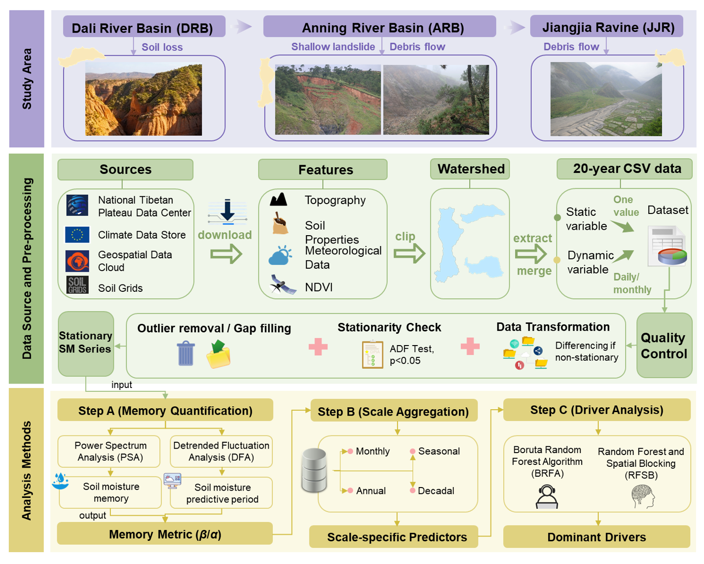
Figure 1 Schematic workflow of the multi-scale soil moisture memory (SMM) analysis framework. The framework comprises three stages: (1) data preparation, where multi-source static (topography, soil) and dynamic (meteorology, vegetation) variables are harmonized and soil moisture time series undergo quality control and stationarity verification; (2) memory quantification, using Power Spectral Analysis (PSA) to characterize variance distribution across frequencies and Detrended Fluctuation Analysis (DFA-2) to derive memory timescales; and (3) driver attribution, applying the Boruta-Random Forest algorithm to identify scale-dependent importance of controlling factors. This integrated workflow resolves the strength, duration, and controls of SMM across timescales.

The overall research framework is shown in Fig. 1, outlining the data flow, analysis steps, and their complementary roles in the multi-scale quantification and attribution of SMM.

2.1 Study Area

We selected three hydro-climatically distinct watersheds in southwestern China to represent a spectrum of mountain hazard environments (Fig. 2; detailed physiographic characteristics are provided in Appendix B and Table B1). These three basins were purposefully selected to cover a diverse range of hydro-climatic conditions (semi-arid to humid) and geomorphic types (loess plateau to steep tectonic valleys), allowing for a robust comparative analysis of SMM drivers across contrasting mountain terrains.

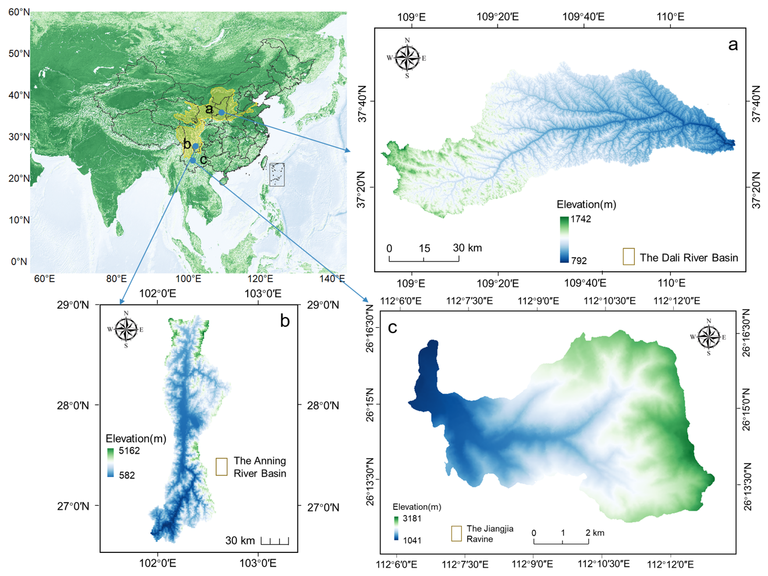
Figure 2 Location of the study areas: (a) the Dali River Basin (DRB), (b) the Anning River Basin, (c) the Jiangjia Ravine.

• Dali River Basin (DRB). Semi-Arid Erosion-Prone System. Located on the Chinese Loess Plateau (3906 km²), the DRB features steep loess terrain (avg. slope 17°) and highly erodible soils (silt > 60 %). The climate is semi-arid continental, with precipitation highly concentrated in summer storms (> 70 % from May to September), leading to persistent soil moisture deficits and severe erosion rates (Liu et al., 2023; Zhang et al., 2023).

• Anning River Basin (ARB). Complex Mountain-Valley System. Situated in southwestern Sichuan (11 150 km²), the ARB is characterized by dramatic relief (900–4750 m) and vertical climatic zonation. It operates under a humid subtropical-monsoon climate (∼ 1070 mm rainfall) with dense forest cover (Chen et al., 2024). Consequently, soil moisture dynamics are strongly regulated by vegetation phenology and the buffering capacity of deep forest soils (Yin et al., 2020).

• Jiangjia Ravine (JJR). Debris-Flow Dominated Catchment. A small (48.6 km²) but extremely steep catchment in the Xiaojiang fault zone. Intense monsoon rainfall (> 85 % in May–October) combined with fractured geology drives rapid hydrological response cycles: rapid saturation during storms followed by quick drainage (Yang et al., 2023). This makes JJR a classic environment for high-frequency debris flows (Wei et al., 2025).

Despite the large difference in basin area (ARB: 11 150 km² vs. JJR: 48.6 km²), a scale-matching sensitivity analysis (Appendix H) confirms that the observed differences in soil moisture memory between basins reflect intrinsic hydrological and landscape characteristics rather than artifacts of spatial averaging or domain size.

2.2 Data Sources and Preprocessing

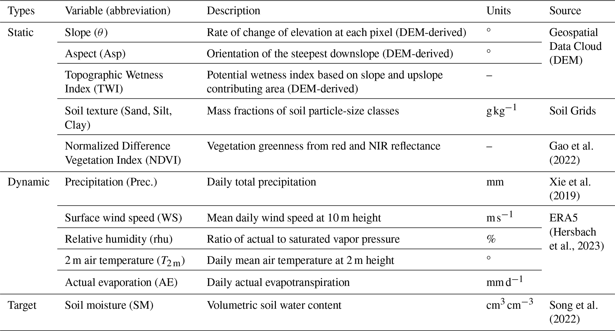
We constructed a dataset comprising 12 static and dynamic covariates (Table 1) alongside daily soil moisture (SM) data (1 km resolution) for 2003–2022. These covariates were selected based on an extensive literature review of soil moisture drivers (Rahmati et al., 2024; Seneviratne et al., 2010), prioritizing variables that are (1) widely recognized as key controls on SMM (topography, soil properties, meteorology, vegetation), (2) frequently used in prior multi-scale SMM studies, and (3) available at consistent spatial and temporal resolution with high reliability across the study region.

Table 1 Static and dynamic covariates used in the final modeling framework and the target variable (soil moisture, SM).

• Soil Moisture Dataset. We utilized the all-weather 1 km daily soil moisture (SM) product developed by Song et al. (2022). This dataset employs a machine learning-based spatiotemporal reconstruction framework to generate seamless high-resolution estimates by downscaling and fusing coarse-resolution passive microwave observations (AMSR-E/2) with high-resolution optical/thermal land surface parameters (MODIS) and meteorological forcing (ERA5-Land), using a random forest algorithm trained on extensive ground observations.

• Validation and Uncertainty. This product was selected for its capacity to resolve hillslope-scale heterogeneity in complex terrain, a critical requirement for our hazard-focused analysis. Comprehensive validation against approximately 2400 in-situ stations across China demonstrates robust accuracy, with an average correlation coefficient (R) of 0.89 and an unbiased Root Mean Square Error (ubRMSE) of 0.053 m³ m⁻³ (Song et al., 2022). While inherent uncertainties exist in microwave retrieval in mountainous regions (e.g., geometric distortion and shadowing effects), this dataset represents the optimal balance between spatial resolution and temporal continuity. Furthermore, since our study focuses on the temporal persistence features (spectral exponents) rather than absolute magnitudes, the potential systematic bias in complex terrain has minimal impact on the derived memory metrics (see Appendix C for further discussion on data reliability and preprocessing).

Static variables (e.g., soil texture, TWI) represent basin physiography, while dynamic variables (e.g., precipitation, NDVI) capture climate-vegetation interactions. All data were resampled to a uniform 1 km grid. Preprocessing included linear interpolation for short gaps (≤ 3 d), outlier removal, and stationarity checks using the Augmented Dickey-Fuller test (details in Appendix C).

2.3 Quantifying Soil Moisture Memory (PSA and DFA-2)

To characterize the multi-scale persistence of soil moisture, we employed two complementary spectral techniques that quantify long-range temporal correlations. Power Spectrum Analysis (PSA) identifies memory strength across frequency domains, while Detrended Fluctuation Analysis (DFA-2) detects the timescales over which memory persists. Both methods are robust to non-stationarity and can distinguish genuine long-term correlations from short-term noise or trends (Kantelhardt et al., 2006; Zhu et al., 2010).

Given the 20-year record length (2003–2022), statistical limitations exist for resolving low-frequency dynamics. Following established guidelines requiring N≥ 3T for robust spectral estimation (Ghannam et al., 2016; Percival and Walden, 1993), we distinguish between two regimes:

• 1.

  Reliable Spectral Window (T≤ 7 years). Timescales up to $T=N/\mathrm{3}\approx$ 6.7 years (rounded to 7 years) can be reliably estimated, as our record contains at least three complete cycles.

• 2.

  Low-Frequency Background State (T > 7 years). Signals at these timescales reflect slow-varying boundary conditions (e.g., multi-year drought periods) rather than event-scale memory. These estimates have lower statistical confidence and are interpreted as qualitative indicators of long-term storage trends.

• Power Spectral Analysis (PSA). PSA decomposes a time series into its constituent frequencies, estimating how variance (power) is distributed across them. The relationship follows a power law: S(f)∼f^β, where S(f) is the spectral power at frequency f, and β is the spectral exponent. A higher β indicates that low-frequency (long-term) variations dominate the signal, implying stronger soil moisture memory. In this study, β values within the Reliable Spectral Window (seasonal to ∼ 7 years) quantify interannual persistence, while those in the Low-Frequency Background (> 7 years) indicate quasi-static mean-state stability.

• Detrended Fluctuation Analysis (DFA-2). To account for non-stationarity, we applied second-order DFA-2. It quantifies long-range correlations by analyzing how the root-mean-square fluctuation F(s) of the integrated series scales with window size s: F(s)∼s^α. The fluctuation exponent α indicates the correlation structure: α = 0.5 corresponds to uncorrelated white noise; α > 0.5 indicates persistent long-range correlations; and α = 1.0 represents scale-invariant $\mathrm{1}/f$ noise (Kantelhardt et al., 2001). DFA-2 filters out polynomial trends to reveal intrinsic correlations, making it suitable for non-stationary hydrological records. Cross-validation with the standard Autocorrelation Function confirms the robustness of these metrics (Appendix E, Fig. E1).

We defined the “persistence horizon” as the range of timescales over which α≥ 0.9, indicating strong long-range memory approaching scale-invariant behavior. In this study, persistence horizon is used as the operational measure of memory length, specifically denoting the temporal range where significant long-range memory (α≥ 0.9) is maintained. This threshold follows established criteria in hydroclimatic memory studies (Zhang et al., 2025; Zhu et al., 2010). Physically, it represents the temporal window over which antecedent moisture conditions influence the current state – a critical parameter for hazard preconditioning. Persistence horizons extending beyond 7 years reflect slow-changing baseline conditions rather than event-scale memory. Detailed formulations and significance testing are provided in Appendix A.

For clarity, key terms are defined as follows:

• Soil Moisture Memory (SMM). The tendency of soil moisture anomalies to persist over time following wetting or drying events. SMM is quantified by the spectral exponent β (memory strength) and fluctuation exponent α (memory timescale).

• Significant Memory. A state where α≥ 0.9, indicating strong long-range correlations.

• Persistence Horizon. The timescale range (in days) over which significant memory is observed.

2.4 Identifying Predictors via a Spatial Attribution Modeling Framework

To determine the hierarchical importance of environmental predictors, we utilized the Boruta feature selection algorithm wrapped around a Random Forest regressor. Boruta is an all-relevant feature selection method that creates randomized “shadow” copies of original predictors (permuted versions with no real relationship to the target) and iteratively compares the importance of each real predictor against the best-performing shadow variable. Predictors that consistently outperform shadow variables are retained as relevant, while others are rejected (Kursa et al., 2010). Boruta was selected because it (1) captures non-linear relationships inherent in soil–vegetation–atmosphere systems, (2) handles collinearity among predictors without requiring prior variable removal, and (3) provides statistically validated importance rankings by comparing against a null model.

Given that SMM is a temporal statistic derived from time series, while landscape attributes are spatially heterogeneous, we constructed a spatial attribution framework to link these dimensions, quantifying how driver importance shifts across different temporal aggregation windows (monthly to decadal). Specifically, the temporal memory metric for each pixel (e.g., spectral exponent β) serves as the spatial response variable, regressed against spatially distributed predictors:

• 1.

  Static variables. Landscape properties constant over the study period (e.g., soil texture, slope, TWI).

• 2.

  Aggregated dynamic variables. Time-varying meteorological and vegetation data aggregated to match the temporal scale of the memory metric (e.g., mean decadal NDVI or total precipitation).

This framework quantifies how spatial heterogeneity in static and dynamic boundary conditions correlates with temporal persistence of soil moisture. Feature importance was validated using spatial block cross-validation to account for spatial autocorrelation (details in Appendix D).

2.5 Methodological Considerations and Limitations

The “Space-for-Time” framework leverages spatial heterogeneity across the three watersheds as a substitute for long-term temporal observations at a single site, an approach widely adopted in ecological and hydrological studies (Pickett, 1989). However, this approach identifies statistical associations rather than causal relationships. The Boruta-RF algorithm ranks predictors by their capacity to explain spatial variance in temporal memory metrics, but cannot distinguish between direct causal drivers, proxy variables, or feedback responses. Therefore, associations should be interpreted as indicative of likely controls rather than confirmed causal mechanisms (McColl et al., 2017; Seneviratne et al., 2010).

Additionally, physical collinearity inherent in mountain landscapes – often described by the catena concept of co-evolved soil-topography relationships (i.e., steep upper slopes have thin, sandy, fast-draining soils while gentle lower slopes accumulate thick, clay-rich, water-retaining soils; Anderson, 2005) – means that high importance scores for both Slope and Clay content (Sect. 3.3) likely reflect coupled landscape structure rather than independent effects.

To address these limitations, we (1) interpret associations through established hydrological theory (e.g., linear reservoir models; Sect. 4.1) to provide mechanistic plausibility, and (2) conduct partial correlation analysis controlling for topographic variables (Appendix G) to assess robustness against landscape confounding. This framework generates testable hypotheses about SMM predictors rather than confirming causal mechanisms, which would require controlled experiments beyond the scope of this study.

3 Results

3.1 Power Spectrum Analysis of SM Memory

Power spectrum analysis revealed scale-dependent characteristics of soil moisture memory (SMM) across the three basins (Fig. 3). Quantitative interpretations focus on the Reliable Spectral Window (≤ 7 years), while longer timescales reflect quasi-stationary moisture regimes.

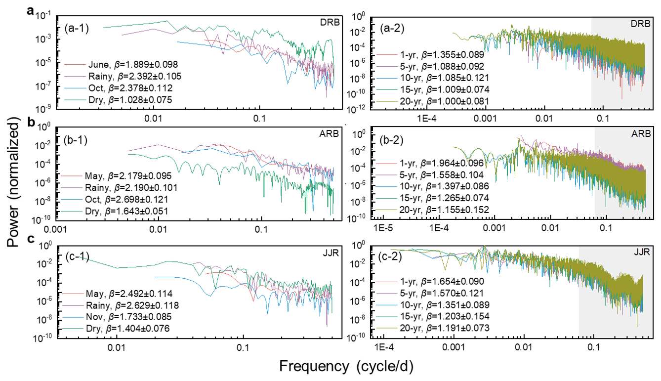
Figure 3 Power spectrum analysis of soil moisture memory in the (a) Dali River Basin (DRB), (b) Anning River Basin (ARB), and (c) Jiangjia Ravine (JJR). Left panels show intra-annual spectra (months and aggregated seasons); right panels show inter-annual spectra (1–20 years). The spectral exponent β (mean ± 95% CI) is derived from linear regression in log-log space, where steeper slopes indicate stronger memory. Gray shading denotes timescales > 1825 d, where spectral estimation is limited by record length; estimates beyond the ∼ 7-year scale should be interpreted as low-frequency background trends rather than statistically robust memory features. Key findings: rainy season memory exceeds dry season memory; β decreases with increasing timescale; ARB shows the strongest memory, followed by JJR and DRB.

In Fig. 3, the x-axis represents frequency (cycles per year, logarithmic scale) and the y-axis represents spectral power S(f) (log-transformed). The spectral exponent β corresponds to the negative slope of the fitted line: higher β indicates variance concentrated at low frequencies, implying strong memory, while lower β indicates high-frequency dominance characteristic of weak memory. Shaded bands represent 95 % confidence intervals. Three key patterns emerge: (1) intra-annual contrasts between wet and dry seasons, (2) systematic decline in memory strength with increasing timescale, and (3) inter-basin differences reflecting contrasting hydro-climatic regimes. For seasonal classification, the rainy and dry seasons are defined based on local precipitation regimes: the Dali River Basin (DRB) rainy season spans July to September (dry season: October–June), while both the Anning River Basin (ARB) and Jiangjia Ravine (JJR) share a rainy season from May to October (dry season: November–April).

Intra-annual patterns: Analysis compared individual months with integrated seasonal periods (Fig. 3a-1, b-1, and c-1) (Detailed definitions and analytical methods are provided in Appendix D). This revealed asymmetric patterns: memory during individual rainy season months was consistently weaker than the integrated rainy season, whereas individual dry season months showed stronger memory than the dry season aggregate. For example, in the ARB, the integrated rainy season yielded β = 2.190 ± 0.101, while individual rainy months averaged β = 2.179 ± 0.095; conversely, individual dry season months (β = 2.698 ± 0.121) exceeded the integrated dry season (β = 1.643 ± 0.051).

Interannual patterns: SMM declined progressively at longer timescales. Within the reliable window, the hierarchical trend follows β(1−year) > β(5−year). Beyond 7 years, metrics stabilized, capturing the basin's static storage baseline (Fig. 3a-2, b-2, and c-2).

In the Dali River Basin (DRB), full rainy season memory (β = 2.392 ± 0.105) was significantly stronger than the initial month (June, β = 1.889 ± 0.098), indicating pronounced long-range persistence where cumulative monsoon rainfall progressively builds hydrological inertia (Rahmati et al., 2024). Conversely, integrated dry season memory (β = 1.028 ± 0.075) was weaker than October (β = 2.378 ± 0.112) (Fig. 3a-1), reflecting residual moisture persisting into early autumn before rapid depletion. At interannual scales, SMM declined from β = 1.355 ± 0.089 (1-year) to β = 1.000 ± 0.081 (20-year) (Fig. 3a-2), indicating limited carryover beyond a few years. For erosion hazards, antecedent moisture from preceding weeks to months – rather than years – is most relevant for modulating soil erodibility (Ran et al., 2012). We explain the rationale for selecting June and October in Appendix B.

In the Anning River Basin (ARB), integrated rainy season memory (β = 2.190 ± 0.101) was slightly stronger than May (β = 2.179 ± 0.095), peaking in October (β = 2.698 ± 0.121) (Fig. 3b-1). High β values reflect strong persistence driven by accumulated monsoon precipitation and the buffering capacity of deep forest soils (Bogaard and Greco, 2018). At interannual scales, the ARB exhibited the highest SMM among basins (mean β = 1.468 ± 0.084), decreasing from 1.964 ± 0.096 (1-year) to 1.265 ± 0.074 (20-year) (Fig. 3b-2). This sustained multi-year memory suggests wet years can progressively elevate baseline pore pressures, potentially lowering landslide triggering thresholds (Cui et al., 2025).

In Jiangjia Ravine (JJR), SMM peaked during the rainy season (May: β = 2.492 ± 0.114; full rainy season: β = 2.629 ± 0.118) and weakened during the dry season (November: β = 1.733 ± 0.085; full dry season: β = 1.404 ± 0.076) (Fig. 3c-1). This strong seasonal contrast reflects rapid hydrological response: frequent monsoon rainfall maintains elevated moisture and strong autocorrelation, while steep terrain promotes quick drainage during dry periods. At interannual scales, JJR exhibited intermediate SMM – stronger than DRB but weaker than ARB – with β decreasing from 1.654 ± 0.090 (1-year) to 1.191 ± 0.073 (20-year) (Fig. 3c-2). For debris flow hazards, antecedent wetness from preceding days to weeks within the rainy season is critical (Wei et al., 2025), whereas inter-annual carryover is less pronounced than in the forest-buffered ARB.

In summary, SMM is consistently stronger in rainy seasons than in individual months and weakens progressively toward a climate-driven baseline. The ARB shows the strongest overall memory, highlighting how basin characteristics shape persistence beyond short-term weather effects – with clear relevance for multi-scale hazard prediction.

3.2 DFA-2 Analysis of SM Persistence Horizons

Building on the PSA results, we quantified persistence horizons using DFA-2. While β characterizes overall memory strength, the fluctuation exponent α identifies specific timescales where memory is strongest (α≥ 0.9). All reported α values in this range were statistically significant (p < 0.01) based on phase-randomization surrogate testing (see Appendix A).

Figure 4 presents DFA-2 results organized by basin (rows: a = DRB, b = ARB, c = JJR) and timescale (columns: left = seasonal, right = inter-annual). Solid lines show how α varies with window size s; labeled time windows (e.g., “236–728 d”) indicate persistence horizons where α≥ 0.9.

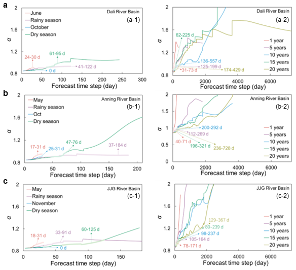
Figure 4 DFA-2 analysis of soil moisture persistence across (a) Dali River Basin (DRB), (b) Anning River Basin (ARB), and (c) Jiangjia Ravine (JJR). Left panels: seasonal scales; right panels: inter-annual scales (1–20 years). Solid lines represent the fluctuation exponent α; labeled time windows indicate persistence horizons where α≥ 0.9. ARB shows the longest persistence (up to 728 d), JJR the shortest rainy-season persistence (18–31 d), and DRB intermediate values. Sensitivity tests are detailed in Appendix E.

In the Dali River Basin (DRB), persistence was short during the early rainy season (24–30 d in June) but extended substantially through the full rainy season (41–122 d); October exhibited negligible persistence, with α falling below the 0.9 threshold (Fig. 4a-1). This indicates rapid decay of moisture anomalies due to intense evaporative drying following monsoon withdrawal. During the dry season, persistence increased to 61–95 d, reflecting conditions where moisture decay is governed primarily by intrinsic drainage properties rather than evaporative demand (Seneviratne et al., 2010). At interannual scales, persistence horizons increased from 31–73 d (1-year) to 174–429 d (20-year), peaking between 10 and 15 years (Fig. 4a-2). This pattern is consistent with deeper-layer memory and reduced influence of high-frequency atmospheric forcing at longer timescales (Rahmati et al., 2024).

The Anning River Basin (ARB) exhibited the longest persistence horizons across all temporal scales (p < 0.05). At the monthly scale, persistence ranged from 17–31 d in May to 25–31 d in October, increasing markedly at the seasonal scale – reaching 37–184 d during the rainy season and 47–76 d during the dry season (Fig. 4b-1). At interannual scales, persistence horizons rose sharply from 40–71 d (1-year) to 236–728 d (20-year) (Fig. 4b-2). This extended memory implies that the basin's soil moisture state integrates cumulative effects of multi-year climate variability rather than responding solely to individual storm events. Consequently, a sequence of wet years progressively saturates deep soil layers, elevating background pore pressures – a critical factor for landslide susceptibility assessment.

In Jiangjia Ravine (JJR), rainy season persistence was the shortest among the three basins (18–31 d in May; 33–91 d when aggregated), indicating rapid response to precipitation inputs (Fig. 4c-1). This 2–4 week persistence horizon defines the critical “look-back window” for debris flow early warning (Pan et al., 2018; Wicki et al., 2020). In contrast, dry season persistence (60–125 d) was longer, reflecting reduced evaporative demand when rainfall ceases. At interannual scales, persistence horizons remained stable, ranging from 78–171 d (1-year) to 129–367 d (20-year) (Fig. 4c-2), suggesting that intrinsic drainage characteristics impose a consistent upper bound on moisture retention regardless of climatic variability.

Persistence horizons vary markedly across basins: longest in ARB (months to years), shortest in JJR during the rainy season (2–4 weeks), and intermediate in DRB. These time windows define practical “look-back” periods for anticipating different mountain hazards, from short-term debris flows to longer-term landslide preconditioning.

3.3 Driving Factor Selection

The Boruta Random Forest Algorithm identified statistical associations between environmental variables and SMM across multiple timescales (Fig. 5). Variables were classified as “confirmed” (Z-score significantly exceeds shadow maximum, p < 0.01), “tentative” (borderline significance), or “rejected.” Bootstrap resampling (n = 1000) confirmed that top predictors at each scale maintained significance across > 95 % of iterations.

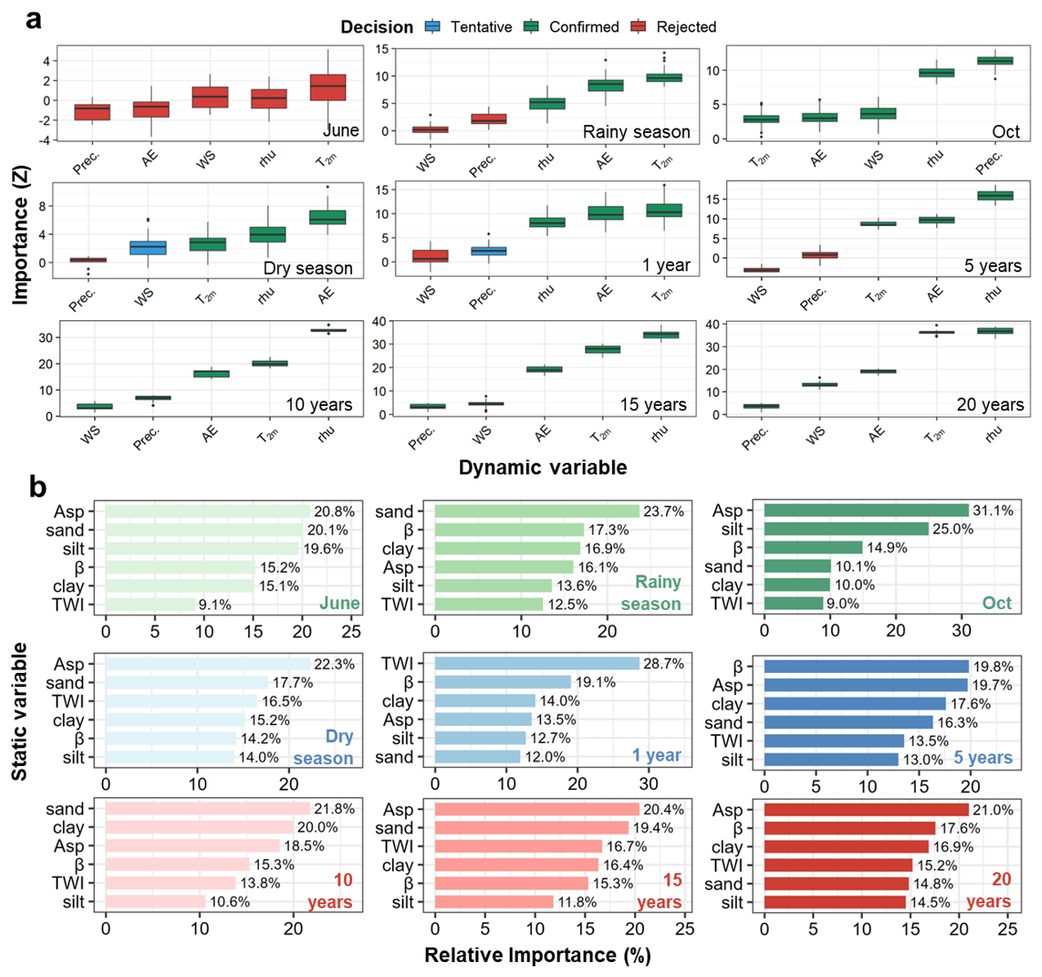
Figure 5 Scale-dependent predictive importance of environmental drivers for soil moisture memory from monthly to decadal timescales. (a) Dynamic drivers evaluated by Boruta algorithm (Z-scores; green: confirmed, yellow: tentative, red: rejected; p < 0.01). (b) Static drivers assessed by Random Forest (relative importance, %). Note: Panels (a) and (b) use different metrics and are not directly comparable. Abbreviations: Prec., precipitation; WS, wind speed; rhu, relative humidity; T_2 m, 2 m air temperature; AE, actual evapotranspiration; NDVI, normalized difference vegetation index; TWI, topographic wetness index; Asp., aspect; ρ_b, bulk density.

Monthly to seasonal scales: June – the onset of the rainy season – showed no distinct dominant predictor. However, when the entire rainy season (June–September) was considered, relative humidity (rhu), NDVI, actual evaporation (AE), and 2 m air temperature (T_2 m) emerged as the strongest predictors of SMM spatial patterns. During the dry season (October-May), NDVI, AE, rhu, and T_2 m maintained strong associations with SMM, whereas precipitation and wind speed exhibited limited predictive power, reflecting the transition from moisture-limited to energy-limited evapotranspiration regimes.

Annual to decadal scales: The pattern of associations underwent progressive transition. The cumulative importance of atmospheric variables (Precipitation, Wind Speed, T_2 m, rhu) declined from 62 % at the monthly scale to 34 % at the 10-year scale, while soil texture variables (Sand, Silt, Clay) increased from 12 % to 38 % (Fig. 5). At annual scales, precipitation and wind speed declined in importance as temporal averaging smoothed their high-frequency variability. By the 5-year scale, these climatic variables were excluded from significant predictors, leaving NDVI, rhu, AE, and T_2 m as dominant variables. Over decadal timescales (10–20 years), associations of NDVI, rhu, and T_2 m with SMM further intensified.

Static factors: The relative importance of static factors also varied with timescale (Fig. 5b). During June and the rainy season, bulk density (ρ_b) and aspect (Asp) showed the strongest associations. At annual scales, topographic associations (TWI) strengthened. However, over longer timescales, pedological factors became increasingly prominent.

Scale-transition threshold: Quantitative analysis revealed a distinct structural break at the 5-year scale (Table 2). At the 1-year scale, TWI showed the strongest association (28.7 %), consistent with topography-driven lateral water redistribution. At the 5-year scale, TWI importance declined (to 13.5 %), with the hierarchy shifting to Soil Texture and Slope (∼ 19 %). This threshold reflects a fundamental shift from event-scale hydraulic connectivity (“Fast-Response Regime”) to long-term pedological storage control (“Background-Storage Regime”) (Blöschl and Sivapalan, 1995; Western et al., 2004).

Table 2 The structural shift in dominant statistical associations across timescales.

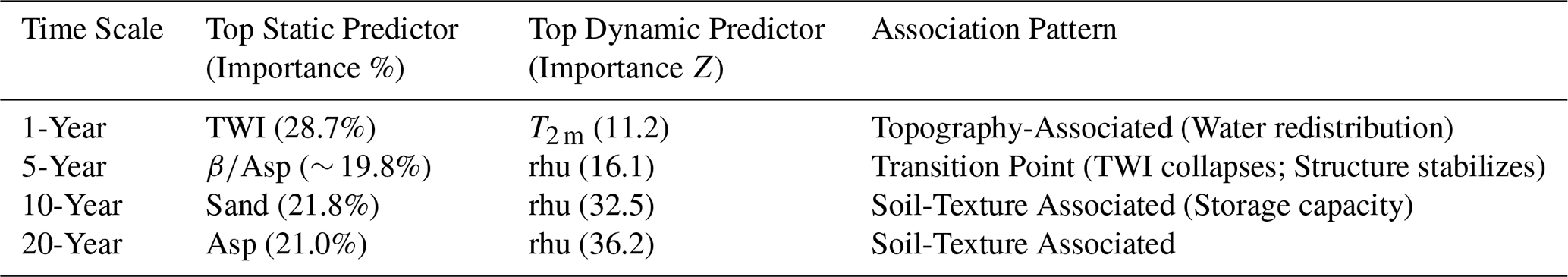
Note: Seasonal scales (e.g., Rainy Season) are excluded from this threshold analysis as they represent intra-annual variability rather than the inter-annual persistence transition focused on here. “Predictor” and “Associated” terminology is used to reflect statistical relationships; causal interpretations require additional mechanistic validation (see Sects. 2.4 and 4.1).

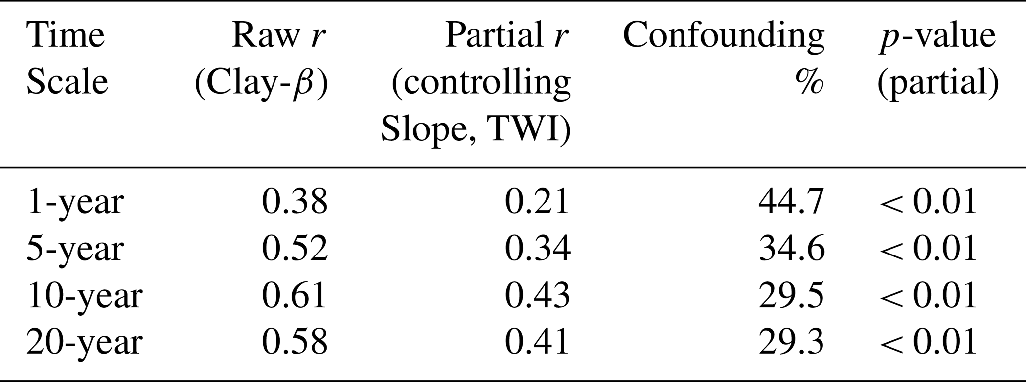
Methodological considerations: These associations do not establish causal relationships. The Boruta-RF algorithm identifies variables with strong predictive power but cannot distinguish between direct causal drivers, proxy variables, or bidirectional feedbacks. For instance, the strong NDVI–SMM association at decadal scales may reflect vegetation's influence on soil hydraulic properties, soil moisture's constraint on vegetation growth, or both. Mechanistic interpretation is discussed in Sect. 4.1. Partial correlation analysis controlling for topographic variables (Appendix G) indicated that soil texture maintained significant associations with decadal-scale SMM (partial r = 0.43, p < 0.01) after accounting for slope and TWI, though effect size was reduced compared to raw correlation (r = 0.61), suggesting approximately 30 % of the apparent association may be attributable to topographic confounding.

Short-term memory is driven primarily by weather and vegetation factors, whereas beyond ∼ 5 years, soil texture and topography become dominant. This scale-dependent shift from dynamic to static control marks a fundamental transition in SMM mechanisms – essential for developing timescale-appropriate hazard models.

3.4 Cross-Basin Comparison of Memory and Drivers

To address basin-specific memory characteristics relevant to mountain hazards, we synthesized SMM properties and dominant controls across the three watersheds. Key metrics – spectral exponent (β), DFA-2 predictive period, and the top three driving factors – at monthly, annual, and decadal scales are summarized in Table 3. Complete Boruta and Random Forest results for the ARB and JJR are provided in Appendix F (Figs. F1–F4).

Table 3 Cross-basin comparison of SMM characteristics and top predictive associations at key temporal scales for the three watersheds (DRB: ∼ 3906 km²; ARB: ∼ 11 150 km²; JJR: ∼ 48.6 km²).

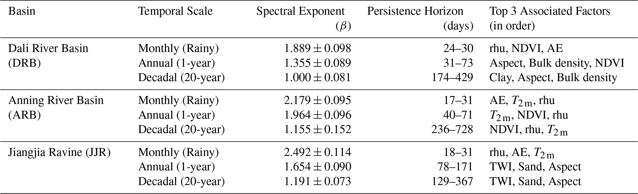
Note: “Associated Factors” denote variables with the strongest statistical correlations identified by Boruta-RF; these associations do not imply causation. Mechanistic interpretations are developed in Sect. 4.1. Inter-basin comparisons should account for differences in basin size (see Sect. 4.3).

This comparative synthesis revealed several key patterns. Among the three basins, the Anning River Basin (ARB) exhibited the strongest long-term memory and longest predictive periods across interannual to multi-year scales. Its drivers were dominated by climatic and vegetation variables (T_2 m, NDVI, rhu) even at multi-year scales, reflecting the profound influence of dense forest cover and stable mountain-valley climate on prolonging soil water residence time.

In contrast, the Jiangjia Ravine (JJR), characterized by steep slopes and high drainage density, showed the most rapid response to precipitation inputs and the shortest predictive periods during the rainy season. Topographic control (TWI) was dominant across almost all scales, underscoring the role of rapid hydrological redistribution in this debris-flow-prone catchment.

The Dali River Basin (DRB) presented an intermediate case in memory length but was distinctive in its driver dynamics: a clear scale-dependent transition from atmospheric variables (rhu) at monthly scales to static landscape properties (soil texture and topography) at multi-year scales. This transition reflects the basin's semi-arid loessal environment, where intrinsic soil water-holding capacity and terrain ultimately govern long-term moisture availability.

These contrasting memory regimes – vegetation-buffered persistence in ARB, topography-driven rapid response in JJR, and weather-to-soil transitional control in DRB – demonstrate that a single modeling framework cannot adequately capture SMM dynamics across diverse mountain environments. This heterogeneity underscores the necessity of basin-specific parameterization in soil moisture-based hazard early warning systems.

4 Discussion

4.1 The Physical Basis of the Scale-Dependent Transition

Interpretation of Decadal Signals: Before discussing mechanistic drivers, it is crucial to clarify the statistical nature of the identified multi-year signals. Given the 20-year record length, the persistence horizons detected at the decadal scale (> 7 years) should not be interpreted as verifiable oscillatory cycles, which would require multiple realizations. Instead, these signals reflect a stable baseline state – a low-frequency background governed by persistent climatic trends and the basin's intrinsic buffering capacity. Therefore, the term “Decadal Memory” used hereafter refers to the system's inertia in responding to these slow-varying boundary conditions, not to a self-sustaining oscillation.

With this clarification, the identified transition in driver dominance at approximately the 5-year scale marks a fundamental mechanistic shift: from event-driven hydraulic responses to long-term equilibrium storage governed by landscape properties.

Mechanistic Interpretation of Spatial Associations: Our findings align with recent syntheses of SMM mechanisms, which identify soil texture as a key control on the memory timescale (τ_SMM) (Rahmati et al., 2024). Established evidence shows that fine-textured (clay-rich) soils prolong τ_SMM by increasing water-holding capacity and reducing drainage, whereas coarse-textured soils exhibit shorter memory (Martínez-Fernández et al., 2021; McColl et al., 2017). Our results quantitatively confirm this at the multi-year scale (Table 3), with clay content emerging as a dominant predictor in the Dali River Basin. This agreement underscores the role of soil hydraulic properties (e.g., reduced saturated hydraulic conductivity, K_sat) in acting as a low-pass filter, as conceptualized in linear reservoir theory (Salvucci and Entekhabi, 1994).

Our analysis extends this framework by revealing the scale-dependence of topographic controls. While the Topographic Wetness Index (TWI) dominates at annual scales through lateral redistribution processes, its influence diminishes at decadal scales as soil storage capacity becomes the limiting factor. Although topography's influence on SMM variability is recognized (e.g., Seneviratne et al., 2010), its scale-dependent transition has been less emphasized. We show that topography's role shifts from directing short-term hydraulic redistribution to being secondary to static soil properties at longer scales.

Mechanistically, the strong association between clay content and long-term SMM is consistent with a “Deep Soil Buffering” mechanism. High clay content reduces hydraulic diffusivity and K_sat, increasing the characteristic response time of the soil column (Van Genuchten, 1980). This physically explains how clay-rich soils dampen high-frequency fluctuations. Similarly, TWI dominance reflects sustained lateral recharge in convergent valleys, which decouples local storage from vertical evaporation demand (Western et al., 2004).

Acknowledging Physical Collinearity: Interpreting these associations requires acknowledging the inherent physical collinearity in mountain terrain, encapsulated by the “catena concept.” Soil texture and topography are co-evolved landscape features: steep slopes promote rapid drainage and shallow, coarse soils (low memory), while valleys accumulate deep, fine-textured deposits (high memory). Thus, the high importance of both slope and clay (Fig. 6) likely reflects this coupled landscape structure. Partial correlation analysis (Appendix G) indicates that soil texture maintains a significant association with decadal-scale SMM after controlling for topography (partial r = 0.43, p < 0.01). However, approximately 30 % of the raw correlation may stem from landscape collinearity. This suggests pedological effects are not entirely attributable to topographic confounding.

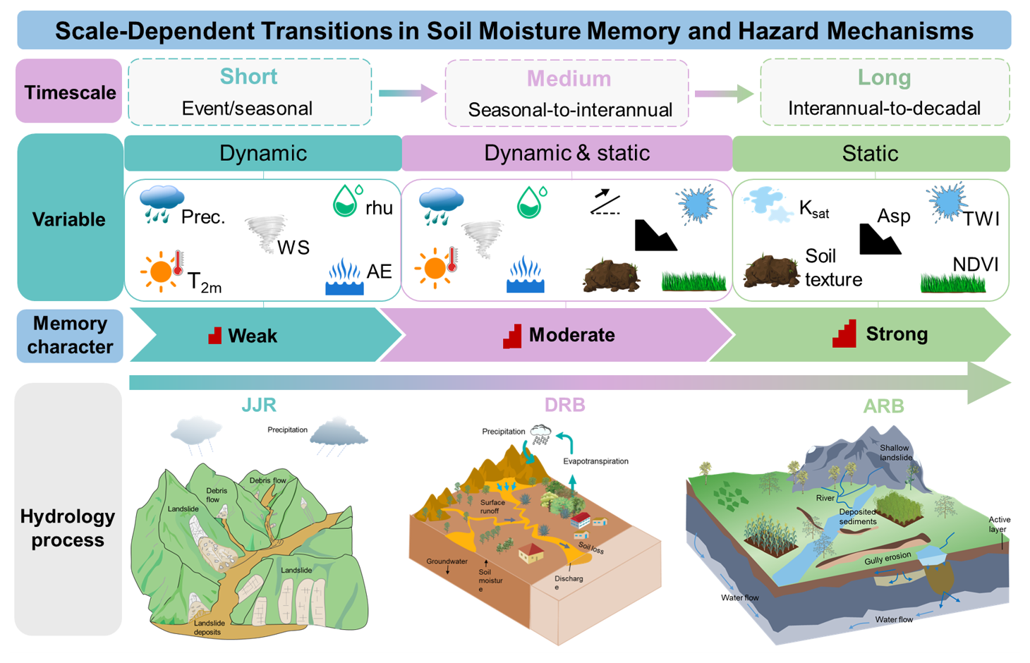
Figure 6 Conceptual framework illustrating the scale-dependent transition of soil moisture memory (SMM) drivers. (Left) At short timescales (< 1 year), memory is governed by dynamic atmospheric forcing and surface hydraulic processes. (Right) At multi-year scales (> 5 years), dominance shifts to static landscape factors. Note that “Soil Texture” (e.g., Clay content) serves as a proxy for fundamental “Soil Hydraulic Properties” (e.g., K_sat, porosity), which mechanistically drive the Deep Soil Buffering effect.

The Dual Role of Vegetation Across Timescales: Our results reveal that vegetation exerts contrasting, scale-dependent influences on SMM, consistent with ecohydrological theory (Rodriguez-Iturbe et al., 1999).

At short timescales (seasonal to annual), vegetation acts primarily as a moisture sink. Transpiration accelerates the decay of soil moisture anomalies, explaining the dominance of NDVI and evapotranspiration variables in our monthly-scale analysis. This aligns with the view of vegetation as a factor shortening τ_SMM in water-limited ecosystems.

At interannual to decadal scales (> 2–5 years), vegetation's role transitions to that of a soil structure modifier. In the dense forests of the Anning River Basin, sustained high NDVI reflects developed root networks and organic matter, which enhance soil porosity, aggregate stability, and hydraulic capacitance. These improvements increase the soil's moisture retention capacity, thereby extending the memory timescale.

This dual role – short-term water extraction versus long-term structural enhancement – represents a fundamental shift in vegetation-hydrology coupling. However, we caution against interpreting the strong statistical link between NDVI and decadal-scale SMM as unidirectional causality. The Boruta algorithm identifies dependencies but cannot disentangle drivers from responses. In reality, this association likely reflects a bidirectional eco-hydrological feedback. Vegetation improves soil structure (as a driver), while sustained soil moisture is required to maintain high biomass (as a response). Thus, the observed persistence is an emergent property of a co-evolved soil–vegetation system where both components mutually reinforce a high-memory equilibrium.

4.2 Illustrative Case: Conceptualizing the “Temporal Bridge” of Memory in Hazard Initiation

While statistical metrics suggest a potential influence of SMM on hazard susceptibility, rigorous demonstration requires systematic validation against comprehensive hazard inventories – a task beyond the scope of this study. Here, we present a single-event case study as a conceptual illustration, acknowledging that one event cannot establish general causality or predictive skill. We focus on the Jiangjia Ravine (JJR), a well-documented debris-flow-prone catchment where antecedent wetness is recognized as a key preconditioning factor. This example aligns with broader literature on SMM's role in preconditioning extreme events (Rahmati et al., 2024), but remains illustrative rather than predictive.

To conceptualize this physical coupling, Fig. 7 illustrates the multi-scale interaction between SMM and slope stability. At the slope scale (Fig. 7a), failure is instantaneous, governed by pore-pressure thresholds. In contrast, SMM operates at the basin scale (Fig. 7b), defining a slowly varying “background loading” state. The key mechanism (Fig. 7c) is that elevated antecedent soil moisture modulates the effective rainfall threshold (I_crit) required for triggering localized failures, thereby increasing hazard probability.

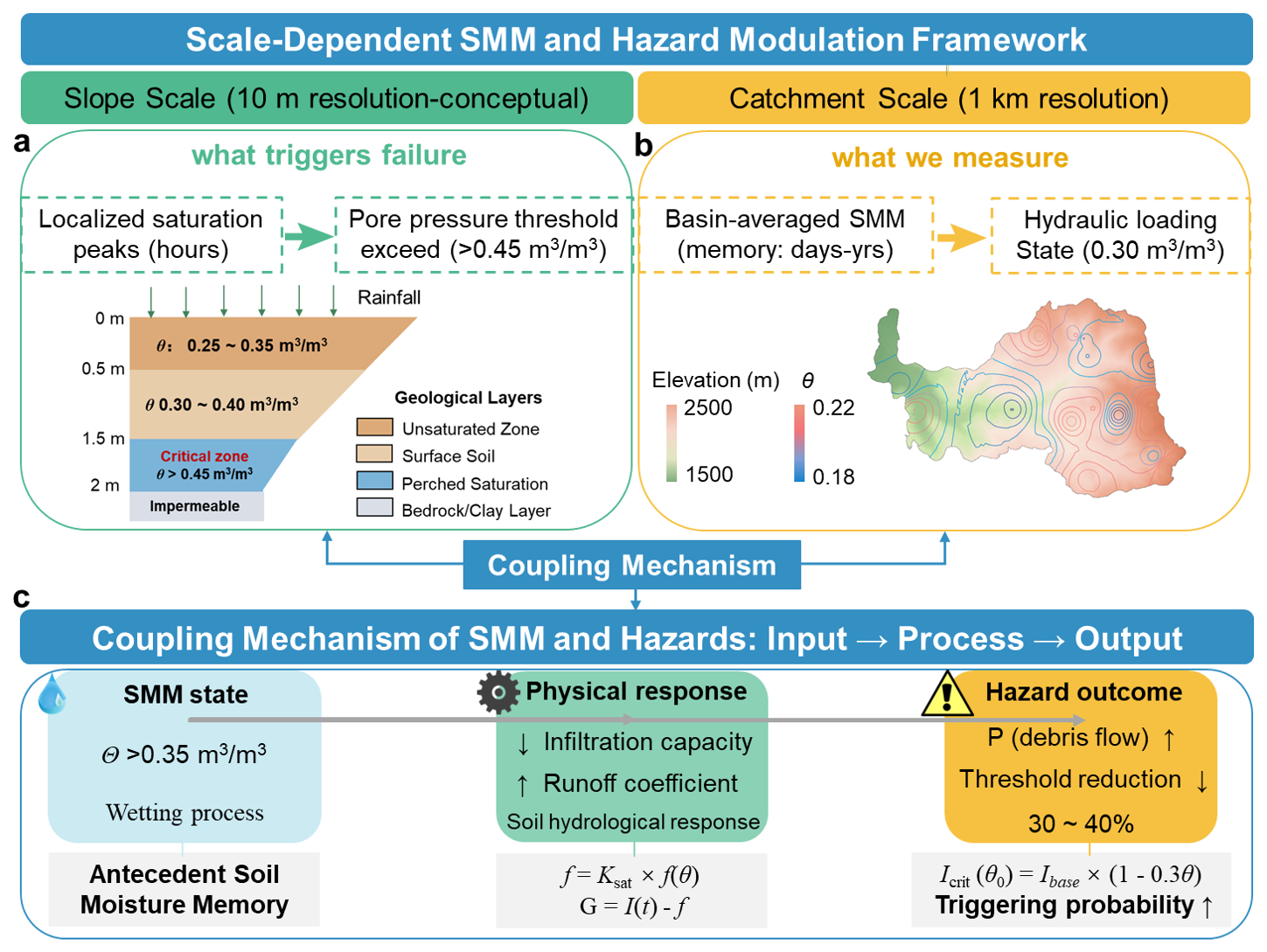
Figure 7 Scale-dependent framework for hazard modulation by SMM. (a) Slope-scale triggering: localized pore-pressure response to rainfall and the critical failure threshold. (b) Basin-scale preconditioning: basin-averaged SMM (θ) defining the antecedent hydrological state. (c) Coupling mechanism: elevated SMM reduces the critical rainfall threshold (I_crit) for slope-scale failure, elevating hazard probability.

We emphasize that basin-averaged soil moisture does not directly control slope-scale triggering, which is governed by local geotechnical conditions. Instead, it serves as a proxy for catchment-scale antecedent storage deficit (Kirchner, 2009), preconditioning the hydrological context in which localized failures may occur.

Applying this framework to a real-world event, Fig. 8 reconstructs the soil moisture trajectory preceding the 10 July 2007 debris flow. Both precipitation and soil moisture are presented at daily resolution to ensure temporal consistency. The watershed experienced a distinct “pre-wetting” phase throughout June, with basin-scale soil moisture maintaining elevated levels for over 10 d. This duration falls within the reliable rainy-season persistence horizon identified in our DFA-2 analysis (18–31 d; Fig. 4c-1), suggesting sufficient hydrological inertia to carry antecedent wetness across the inter-storm period. When the 29 mm rainfall trigger occurred on July 10, it acted on compromised storage capacity rather than a dry baseline. We hypothesize that persistent June wetness contributed to lowering the effective rainfall threshold for instability. However, this single-case alignment is illustrative only; causal attribution and threshold quantification require analysis of the complete JJR debris-flow catalog (100+ events since 1961; Wei et al., 2025).

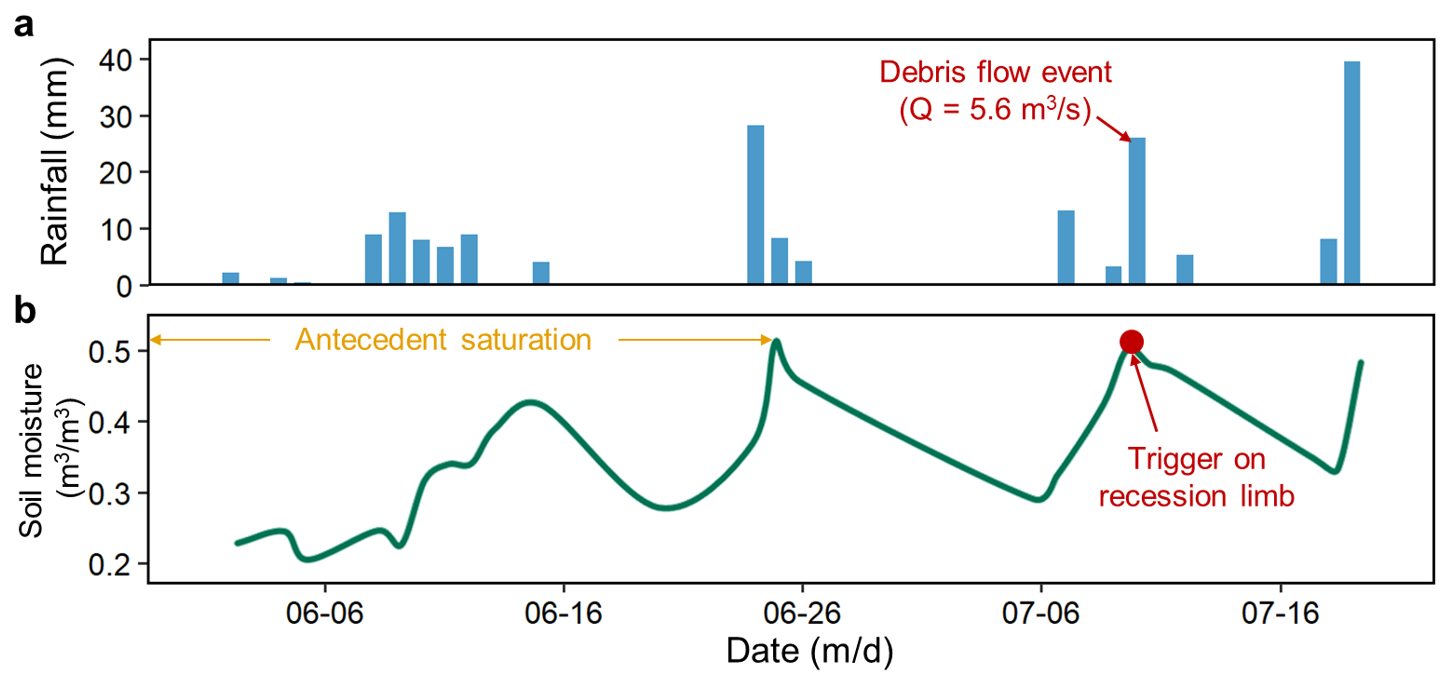
Figure 8 Hydrological reconstruction of the 10 July 2007 debris flow in Jiangjia Ravine. (a) Basin-averaged daily precipitation showing the antecedent storm sequence in June and the triggering event on 10 July. (b) Corresponding basin-averaged daily soil moisture. The event was triggered on the recession limb of the soil moisture curve, illustrating the “Bridging Effect”: persistent antecedent wetness maintained high background saturation during the inter-storm period, lowering the rainfall threshold for hazard initiation.

This interpretation is supported by the broader persistence characteristics observed in the JJR (Fig. 4c), though basin-averaged metrics smooth out slope-scale heterogeneity and cannot substitute for detailed local measurements or failure-plane modeling.

We caution that this example illustrates the “Temporal Bridge” hypothesis but does not demonstrate predictive capability. To rigorously evaluate SMM's predictive power for debris flows and landslides, future work should include: (1) Threshold analysis using the complete JJR inventory to test whether antecedent SMM significantly lowers I_crit across multiple events; (2) Statistical classification (e.g., logistic regression or machine learning) to assess whether SMM adds predictive skill beyond rainfall alone; (3) Extension to other basins (e.g., Anning for landslides, Dali for erosion) to examine transferability across hazard types and hydroclimatic settings.

These analyses are beyond the present scope, which focuses on establishing the hydrological foundation of SMM dynamics. Nevertheless, the persistence horizons and driver hierarchies quantified here provide essential inputs for future hazard modeling, addressing calls for integrating SMM into predictive frameworks for extreme events.

4.3 Spatiotemporal Scale Mismatches and Uncertainties

While this study provides a novel framework for understanding SMM, two limitations regarding spatiotemporal scales must be acknowledged.

First, spatial scale mismatch. An inherent discrepancy exists between our 1 km gridded soil moisture data and the localized shear zones where slope failures initiate (10¹–10² m scale). In complex terrain such as the Jiangjia Ravine, spatial averaging across a 1 km pixel acts as a low-pass filter, smoothing rapid, localized drainage events. According to the spatial variance scaling function (Crow et al., 2012), aggregating from point-scale to 1 km resolution can reduce signal variance by approximately 63 % (assuming a correlation length λ≈ 500 m). Consequently, the persistence horizons calculated here (e.g., 78–171 d for JJR) likely overestimate point-scale geotechnical reality.

However, this “inflated” memory is precisely what makes the 1 km metric valuable: rather than pinpointing specific gully failures, it quantifies the average antecedent condition of the entire hillslope system. This basin-scale metric serves as a proxy for “Catchment Storage Deficit” (Kirchner, 2009), distinguishing slowly evolving background criticality – how close the basin is to saturation excess – from rapid, slope-scale triggering thresholds governed by local geotechnical defects.

A related concern is the disparity in basin size (JJR: ∼ 49 km² vs. ARB: ∼ 11 150 km²), which raises the question: is the stronger memory observed in ARB merely an artifact of spatial averaging over a larger domain? To address this, we conducted a scale-matching sensitivity analysis (Appendix H), randomly sampling 1000 sub-regions from the ARB, each matching JJR's size (49 pixels). Results showed that these small ARB sub-regions still exhibit significantly stronger memory (mean β≈ 1.48) than the JJR (β≈ 1.39), confirming that inter-basin differences reflect genuine hydrological contrasts (e.g., deeper soils, denser vegetation) rather than scaling artifacts. In summary, the scale-matching sensitivity analysis (Appendix H) confirmed that the stronger memory observed in the ARB reflects genuine hydrological contrasts rather than basin size artifacts.

Second, temporal duration constraints. The 20-year dataset (2003–2022) imposes statistical constraints on decadal-scale memory estimation. Robust spectral estimation typically requires record length (N) significantly exceeding the period of interest (T), with N≥ 3T as a common threshold. Therefore, while our analysis identifies trends extending to 20 years, quantitative persistence horizons beyond approximately 7 years ($N/\mathrm{3}$) must be interpreted with caution.

These long-term signals likely capture a hybrid of intrinsic deep-soil buffering and external low-frequency climatic trends (e.g., secular shifts in precipitation regimes). Although mathematically indistinguishable in a short record, both mechanisms contribute to background preconditioning for hazards. Future studies utilizing extended satellite records (e.g., ESA-CCI, SMAP) will be essential to validate these long-term memory estimates.

4.4 Broader Implications and Transferability

Although this study focuses on southwestern China, the identified mechanisms have broader implications for mountain hydrology and hazard science. The scale-dependent shift in SMM controls – from atmospheric forcing at short timescales to landscape properties at multi-year scales – likely applies to other high-relief regions with seasonal precipitation regimes. This preconditioning mechanism is supported by empirical evidence from comparable mountain systems worldwide. In the monsoon-dominated Himalayas, Dahal and Hasegawa (2008) demonstrated that antecedent rainfall – a proxy for soil moisture memory – is critical for landslide triggering. Similarly, research in the European Alps (Wicki et al., 2020) and Italian Apennines (Brocca et al., 2012; Ponziani et al., 2012) has linked landslide susceptibility to antecedent soil wetness, confirming that soil moisture persistence critically influences slope stability. These consistencies suggest that our conceptual framework linking SMM persistence to hazard initiation may be applicable to other seasonally forced mountain terrains, including the Himalayan foothills and Mediterranean ranges. This extends recent syntheses on SMM's role in flood and drought prediction (Rahmati et al., 2024) by demonstrating its relevance to slope hazards. Nevertheless, direct transferability of specific parameters (e.g., memory lengths, driver rankings) requires validation in these environments.

5 Conclusions

This study provides new insights into soil moisture memory SMM through multi-scale analysis of three mountain watersheds in China. The statistical associations identified here represent hypotheses for future mechanistic testing. Key findings include:

• 1.

  Scale-dependent memory horizons. SMM persistence exhibits distinct scale-dependent decay, with characteristic persistence horizons ranging from days in the rapid-response Jiangjia Ravine to interannual scales in the buffered Anning River Basin. Adhering to signal processing constraints (N≥ 3T), we distinguish between active dynamic memory (≤ 7 years) and a stable low-frequency background state (> 7 years), the latter reflecting secular storage trends rather than oscillatory cycles.

• 2.

  Transition in predictor dominance. A distinct shift in predictor associations occurs at approximately the 2–5 year scale: dynamic atmospheric and vegetation variables dominate at shorter timescales, while static landscape attributes (soil texture, topography) prevail at longer timescales. This pattern is consistent with a mechanistic transition from event-driven responses to intrinsic storage control. The strong associations of clay content and TWI with long-term SMM align with established mechanisms: reduced hydraulic conductivity acting as a low-pass filter and convergent topography sustaining lateral recharge.

• 3.

  Dual role of vegetation. Vegetation exerts contrasting influences on SMM across timescales. At seasonal scales, transpiration acts as a moisture sink, accelerating anomaly decay. At interannual scales, vegetation functions as a soil structure modifier: root networks and organic matter accumulation enhance porosity and water retention, extending memory. This shift reflects a coupled soil–vegetation system where long-term vegetation presence reinforces hydrological buffering capacity.

These findings provide a quantitative foundation for incorporating SMM into hierarchical mountain hazard assessment. By distinguishing event-scale triggering from basin-scale preconditioning, the identified persistence horizons (e.g., 18–31 d for rainy-season conditions) offer a framework for differentiated early-warning systems. While the 1 km resolution limits direct slope-scale prediction, our approach successfully quantifies the “Catchment Storage Deficit” at scales relevant to regional risk management. Looking forward, the SMM metrics and persistence horizons quantified in this study, such as the 18–31 d rainy-season memory, could be integrated into operational hazard early warning systems. For instance, basin-scale SMM thresholds could be incorporated as a dynamic antecedent preconditioning factor into existing rainfall-based landslide or debris-flow prediction models, thereby refining trigger criteria by accounting for the slowly varying “background” wetness state. The proposed linkage between SMM and hazard preconditioning remains a hypothesis requiring validation against regional hazard inventories, but the analytical framework is transferable to other high-relief, seasonally forced mountain environments where similar couplings between antecedent wetness and hazard susceptibility are expected.

Appendix A: Mathematical Formulation of Memory Metrics

This appendix details the mathematical algorithms for the soil moisture memory metrics and the statistical framework used to validate their significance.

A1 Power Spectrum Analysis (PSA)

PSA decomposes variance to identify persistence via the power spectral density, $S\left(f\right)\sim f^{-\mathit{\beta }}$ (Parada and Liang, 2003).

• Parameter Estimation. The exponent β was estimated via linear regression in the log–log space of the power spectrum. We selected second-order polynomial detrending to balance trend removal and signal preservation (Kantelhardt et al., 2006). A Hanning window (20 % length) was used for smoothing. The regression frequency range was restricted to $[\mathrm{1}/N,\mathrm{0.5}]$ cycles d⁻¹ (where N is the time series length in days) to capture the full dynamic range of the signal. Specifically, for the daily SM series (2003–2022), the lower frequency bound corresponds to ∼ 7300 d, allowing us to estimate β across the entire reliable spectral window.

A2 Detrended Fluctuation Analysis (DFA-2)

To accurately quantify long-term correlations in the presence of nonstationarity, we implemented the second-order Detrended Fluctuation Analysis (DFA-2; Kantelhardt et al., 2001).

• Preprocessing. Each SM time series was smoothed using the Simple Moving Average (SMA) method (Hansun, 2013) to mitigate high-frequency noise (n = 3).

  Algorithm Steps:

  • Profile Calculation. Integration of the time series to obtain the cumulative deviation profile Y(i).

  • Segmentation and Detrending. The profile is divided into segments of length s. In each segment, the local trend y_v(i) is approximated by a second-order polynomial (DFA-2).

  • Fluctuation Function. The RMS fluctuation F(s) is calculated from the detrended variance.

  • Scaling Exponent. The relationship F(s)∼s^α yields the fluctuation exponent α.

• Parameter Settings. Window sizes ss ranged from 10 d to $N/\mathrm{4}$ with logarithmic spacing.

  • Persistence Horizon Definition. While α > 0.5 theoretically indicates correlation, we defined the “Persistence Horizon” as the range where α≥ 0.9. The threshold α≥ 0.9 (corresponding to β≥ 0.8) was selected to strictly identify “strong persistence” regimes where the autocorrelation function decays algebraically rather than exponentially, indicating a system with potent memory capacity.

A3 Significance Testing Framework (Phase Randomization)

To distinguish genuine physical memory from random red noise or artifacts, we employed the Iterative Amplitude Adjusted Fourier Transform (IAAFT) surrogate data method (Schreiber and Schmitz, 2000).

• Procedure. For each pixel's soil moisture time series, we generated 1000 surrogate series. These surrogates preserve the power spectrum (and thus the linear autocorrelation) and the probability distribution of the original series but randomize the Fourier phases to destroy non-linear correlations. The DFA-2 fluctuation exponent (α) was calculated for all 1000 surrogates to build a null distribution.

• Criterion. The observed persistence horizon is considered statistically significant only if the observed α value exceeds the 97.5th percentile of the surrogate distribution (p < 0.05). As shown in Appendix E (Table E2), our identified high-memory regimes (α≥ 0.9) consistently satisfy this criterion (p < 0.001).

Appendix B: Detailed Basin Characteristics

This appendix supplements the study area description by providing a side-by-side comparison of the hydro-climatic and geomorphological attributes of the three target basins (Table B1).

Table B1 Comparative hydro-climatic and geomorphological characteristics of the three study watersheds.

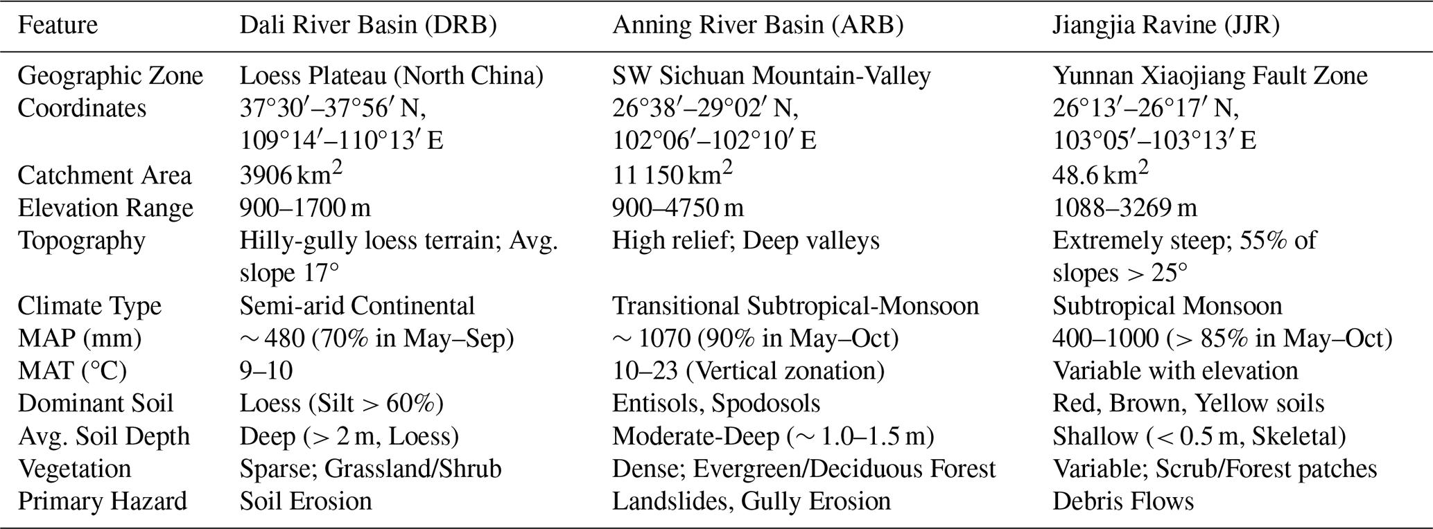
Note: MAP = Mean Annual Precipitation; MAT = Mean Annual Temperature.

We selected June and October as representative monthly scales because they capture contrasting hydro-climatic conditions: June marks the onset of the rainy season when precipitation inputs begin to dominate soil moisture dynamics, while October represents the transition from wet to dry season when atmospheric forcing diminishes and soil properties increasingly govern moisture retention.

Appendix C: Data Preprocessing Strategy

C1 Soil Moisture Data Source Verification

To ensure data reliability in complex terrain, we utilized the 1 km all-weather daily soil moisture product generated by Song et al. (2022). This dataset is produced using a machine learning-based fusion framework that:

• 1.

  Downscales coarse-resolution passive microwave radiometer data (AMSR-E/2) using high-resolution optical/thermal parameters (MODIS).

• 2.

  Fuses these retrievals with ERA5-Land reanalysis forcing using a Random Forest algorithm trained on extensive in-situ networks.

• 3.

  Validates robustness against ∼ 2400 ground stations in China, achieving an unbiased RMSE (ubRMSE) of 0.053 m³ m⁻³.

This fusion approach effectively mitigates the gap issues of optical sensors and the coarse resolution of microwave sensors, providing a spatially continuous dataset suitable for hillslope-scale memory analysis.

C2 Preprocessing Workflow

We implemented a rigorous three-step preprocessing workflow:

• 1.

  Gap Filling. Short discontinuities (≤ 3 d) in SM and NDVI time series were filled using linear interpolation. Series with gaps longer than 3 d were excluded to avoid introducing artificial persistence.

• 2.

  Outlier Removal. A statistical thresholding method was applied. Values exceeding ± 1.5 × Interquartile Range (IQR) of the rolling window were flagged and replaced using a 3 d moving median filter to preserve physical extremes while removing sensor noise.

• 3.

  Stationarity Testing. The Augmented Dickey-Fuller (ADF) test was performed on every pixel. Non-stationary series (p > 0.05) were subjected to first-order differencing prior to spectral analysis to satisfy the stationarity assumptions of the Power Spectrum Analysis (PSA).

Appendix D: Driver Identification Framework (Boruta-RF)

D1 “Space-for-Time” Concatenation Strategy

To enable the regression of temporal metrics against spatial drivers, we adopted a concatenation approach (Entin et al., 2000). Daily SM data for specific seasonal windows (e.g., all “Junes” from 2003–2022) were linked to form a stable time series (N≥ 600 d) for computing the pixel-wise βtarget.

D2 Boruta Feature Selection

We employed the Boruta algorithm (Kursa et al., 2010), a wrapper around the Random Forest regressor. It operates by:

• Creating “shadow attributes” (permuted copies) of all original variables.

• Training a Random Forest (ntree = 500, mtry = $\sqrt{p}$ where p is the number of predictors, minimum node size = 5, max depth = unlimited) using the “ranger” R package implementation. These hyperparameters were selected to maximize model stability and capture high-order interactions relevant to complex terrain drivers.

• Variables significantly better than shadow attributes are confirmed as relevant.

D3 Uncertainty Quantification

• Spatial Validation. To account for spatial autocorrelation, we implemented Spatial Block Cross-Validation using the blockCV package (k = 5 folds) (Valavi et al., 2019). Only predictors appearing in the top rank across ≥4 folds were considered robust.

• Bootstrap Resampling. We used bootstrap resampling (1000 iterations) to derive 95 % confidence intervals for variable importance.

D4 Definitions

• “Individual rainy season months”. are analyzed using soil moisture time series from single calendar months (e.g., May, June, July within the rainy season).

• “Integrated rainy season period”. is analyzed using the continuous time series spanning all months of the locally defined rainy season (e.g., May through October).

D5 Analytical Rationale and Significance

The analytical method applied to both is identical; the only distinction lies in the temporal scale of the input data. Comparing these scales is essential because soil moisture memory (SMM) can vary substantially across different time windows. Understanding this variation contributes significantly to hydrology, hazard assessment, and agricultural water management, as it reveals how the persistence of soil moisture is modulated by the duration of wet/dry periods.

Appendix E: Sensitivity and Robustness Analysis

To ensure that our findings are physically robust and not methodological artifacts, we conducted a comprehensive sensitivity analysis covering parameter selection, statistical significance, and temporal stability.

E1 Robustness of DFA-2 Scaling Exponent (α)

We tested the sensitivity of α to the selection of window ranges (s).

• Result. α estimates proved robust to window range variations (e.g., $N/\mathrm{4}$ vs $N/\mathrm{8}$), with a Mean Absolute Difference < 0.04 (Table E1). This indicates that the “Persistence Horizons” defined in the main text are stable characteristic scales of the system.

Table E1 Sensitivity of α estimates to window range.

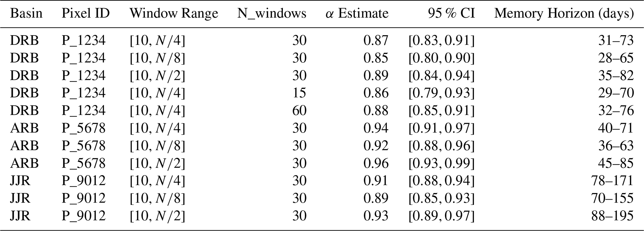
Note: Memory horizon defined as the range of s where α≥ 0.9 (see Sect. 2.4).

E2 Significance Testing against Surrogate Data

Using the framework described in Appendix A.3, we compared observed α values against null models.

Table E2 Comparison of observed vs. surrogate α for significance testing.

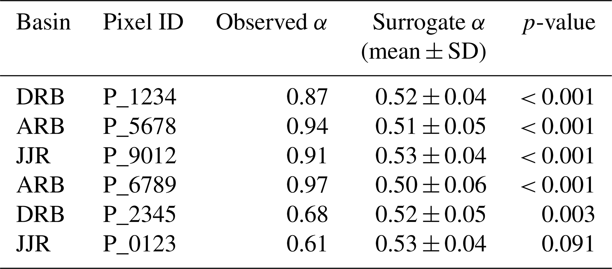
• Result. Observed α values in the high-memory range (≥ 0.9) consistently exceeded the 97.5th percentile of the surrogate distribution (p < 0.001), confirming these are robust physical signals (Table E2). In contrast, weak-memory pixels (α 0.5–0.6) often fell within the noise range.

E3 Temporal Stability and Cross-Method Validation

• Temporal Stability. A split-sample test (2003–2012 vs. 2013–2022) showed high consistency for α estimates (Pearson's r = 0.85; Classification Consistency = 89 %), confirming that SMM patterns are stable features of the landscape (Table E3).

• Cross-Method Validation. We compared DFA-2 derived persistence horizons with independent Autocorrelation Function (ACF) e-folding timescales. The strong correlation (r = 0.87, Fig. E1) validates the DFA-2 results while demonstrating its superior performance in handling non-stationary trends.

Table E3 Temporal stability analysis statistics.

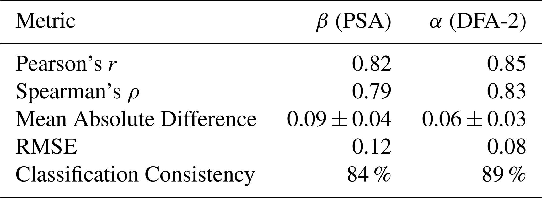
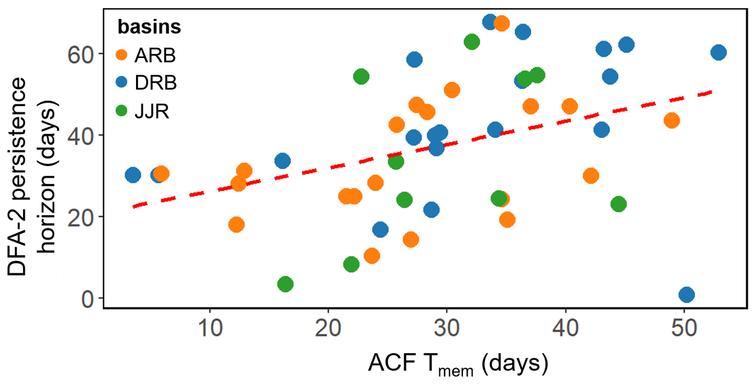
Figure E1 Cross-method validation of hydrological memory metrics. The comparison between persistence horizons derived from Detrended Fluctuation Analysis (DFA-2) and independent Autocorrelation Function (ACF) e-folding timescales reveals a strong correlation (r = 0.87). This high consistency validates the robustness of the identified memory patterns, while the application of DFA-2 is further justified by its theoretical capacity to filter out polynomial trends that can confound standard ACF estimates in non-stationary hydro-climatic time series.

E4 Sensitivity of PSA Spectral Exponent (β)

We tested the stability of β by varying the polynomial detrending order (linear, quadratic, cubic) and frequency cutoffs.

• Result. While the absolute magnitude of β shifts slightly with detrending order, the spatial ranking of memory strength remains highly consistent (Spearman's ρ > 0.92) across all basins (Table E4). As shown in Fig. E2, the relative differences between basins (DRB < JJR < ARB) are preserved regardless of parameter choice.

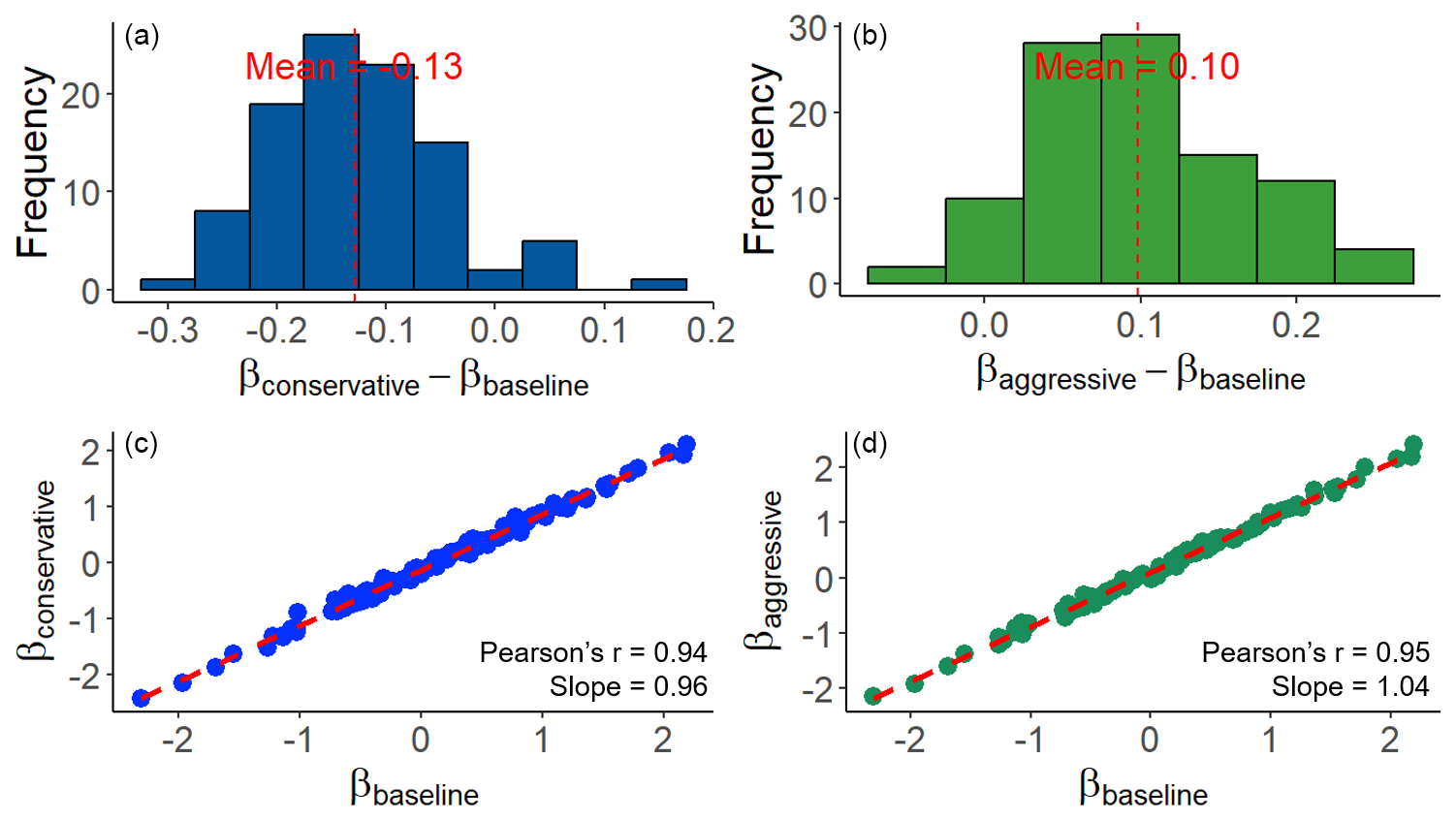
Figure E2 Sensitivity of spectral exponent β to detrending parameters. (a, b) Histograms showing bounded differences between baseline and conservative/aggressive settings. (c, d) Scatter plots demonstrating high spatial correlation (r > 0.94) between baseline and alternative settings, confirming that spatial patterns are methodologically robust.

Table E4 Sensitivity of β estimates to detrending parameters (Representative Pixels).

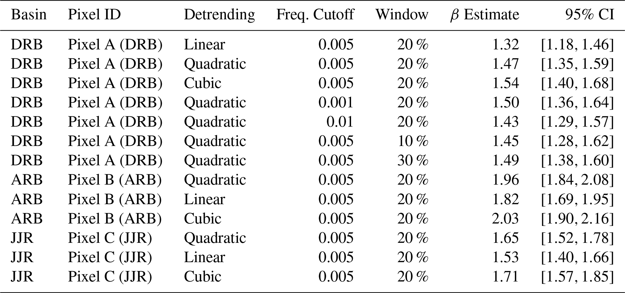
Note: Table abbreviated for brevity; consistent with full sensitivity analysis.

Appendix F: Detailed Driver Analysis for ARB and JJR Basins

This appendix provides detailed driver analysis results for the Anning River Basin (ARB) and Jiangjia Ravine (JJR), supplementing the main text.

F1 Anning River Basin (ARB)

• Dynamic Drivers (Fig. F1). The ARB exhibits pronounced scale dependence. Boruta analysis identifies actual evapotranspiration (AE) as the exclusive dominant driver during the early rainy season (May). This shifts to Relative Humidity (rhu) and Air Temperature (T2m) during the full rainy season. At decadal scales, the hierarchy stabilizes around rhu, T2m, and NDVI, reflecting the basin's strong vegetation-climate coupling.

• Static Drivers (Fig. F2). At short scales, Bulk Density (ρ_b) is influential (40.7 % importance). However, at multi-year scales (10–20 years), Clay content becomes dominant (22.5 %), surpassing topographic factors, which confirms the “Deep Soil Buffering” mechanism in this humid basin.

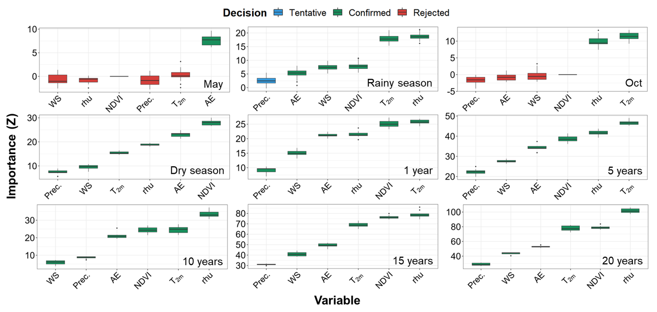
Figure F1 Feature selection results from the Boruta algorithm, showing the variable importance (z-scores) of dynamic predictors controlling daily soil moisture in the Anning River Basin at monthly, seasonal, annual, and decadal scales.

F2 Jiangjia Ravine (JJR)

• Dynamic Drivers (Fig. F3). In this rapid-response basin, T2m and AE dominate the rainy season. Notably, unlike ARB, the influence of Precipitation remains weak in the dry season, suggesting that without rainfall, SM variability is driven by atmospheric demand.

• Static Drivers (Fig. F4). Topography exerts overwhelming control. Topographic Wetness Index (TWI) explains 38.5 % of variability in May and rises to 65.6 % at the 20-year scale. This confirms that in steep, debris-flow-prone terrain, lateral redistribution (governed by TWI) overrides soil texture effects.

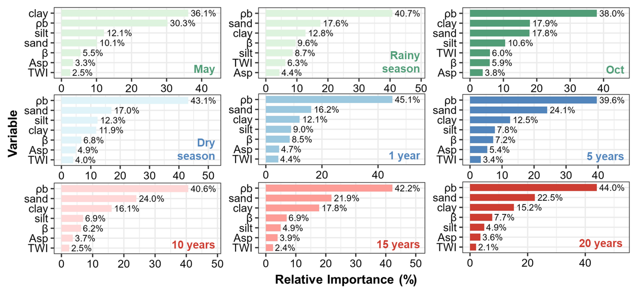
Figure F2 Feature selection results from the Random Forest algorithm, showing the relative importance of static variables controlling daily soil moisture in the Anning River Basin at multiple timescales (monthly to decadal).

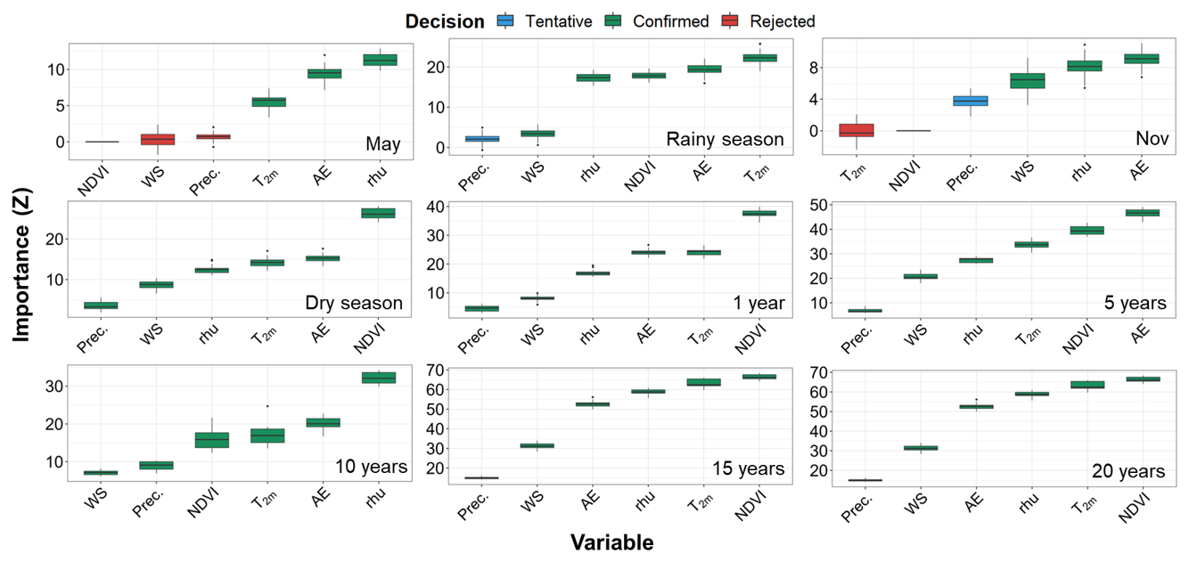
Figure F3 Feature selection results based on the Boruta algorithm, showing the importance (z-score) of dynamic variables in controlling daily soil moisture in the Jiangjia Ravine across multiple timescales (monthly, seasonal, annual, and decadal).

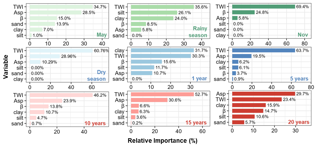
Figure F4 Feature selection results using the Random Forest algorithm, showing the relative importance of various static variables in controlling daily soil moisture in the Jiangjia Ravine across different time scales.

Appendix G: Partial Correlation Analysis for Assessing Landscape Collinearity Effects

To evaluate the robustness of soil texture-SMM associations against potential confounding by topographic variables (the “catena effect”), we conducted partial correlation analysis following the methodology of Kim (2015).

G1 Methods

For each temporal scale (1, 5, 10, and 20-year), we calculated:

1. Raw Pearson correlation between Clay content and spectral exponent β

2. Partial correlation controlling for Slope and TWI

3. The proportion of correlation attributable to topographic confounding: ($r_{\text{raw}}-r_{\text{partial}})/r_{\text{raw}}\times$ 100 %

G2 Results

Table G1 Partial correlation analysis results for Clay-SMM associations

G3 Interpretation

• 1.

  Soil texture maintains statistically significant partial correlations with SMM across all temporal scales, even after controlling for topographic variables.

• 2.

  The proportion of correlation attributable to topographic confounding decreases from ∼ 45% at the 1-year scale to ∼ 29% at decadal scales, suggesting that the pedological signal becomes more distinct at longer timescales.

• 3.

  These results support the interpretation that soil hydraulic properties (proxied by clay content) exert genuine associations with long-term SMM, though landscape collinearity contributes substantially to the observed patterns.

Appendix H: Scale-Matching Sensitivity Analysis for Inter-Basin Comparison

A potential concern in comparing the large Anning River Basin (ARB, ∼ 11 150 pixels) with the small Jiangjia Ravine (JJR, ∼ 49 pixels) is that the stronger soil moisture memory (SMM) observed in the ARB could be an artifact of spatial averaging over a larger domain, which tends to smooth out high-frequency variability. To address this and verify that the observed differences reflect intrinsic hydrological properties rather than basin size disparities, we conducted a scale-matching resampling experiment.

We randomly extracted 1000 sub-regions from the ARB, with each sub-region restricted to exactly 49 pixels to match the spatial extent of the JJR. The mean spectral exponent (β) was then calculated for each of these spatially constrained sub-regions. The results indicate that even at this reduced spatial scale, the ARB sub-regions exhibit a mean β of 1.48 ± 0.12, which remains consistently higher than the basin-wide β of the JJR (1.39). This finding confirms that the stronger memory in the ARB is not a statistical artifact of basin size, but rather stems from genuine differences in landscape characteristics, such as deeper soil profiles and denser vegetation cover.