Modeling E. coli fate and transport in and around a cattle pond

Contamination of surface water is a concern for public health. Lands used for animal production are sources of fecal microorganisms that can reach water bodies, impact their quality, and adversely affect their potential uses. Understanding the mechanisms of microbial transport through surface/subsurface flow is imperative to predict surface water contamination and to assign management strategies for enhanced water quality. The aim of this work was to develop and test a mechanistic numerical model to simulate watershed-scale surface/subsurface water flow, bacteria release from cow manure, and their fate, as well as transport to a cattle pond. The integrated surface-subsurface hydrological platform HydroGeoSphere (HGS) was the basis for the site-specific model. The pond and its environs were monitored for 15 months for Escherichia coli (E. coli) concentrations, which remained relatively high throughout the study. The model was applied to simulate E. coli bacteria transport in a grassed drainage basin grazed by a permanent herd of approximately 50 cattle. Most model parameter values were adopted from the literature. The model explicitly accounted for cow excretion to the pond as a source of microbial contamination. The latter was estimated from the time spent by cows in the pond, which in turn was estimated from imagery obtained with eight trail cameras installed to cover the pond surface. Images were obtained every 15 min. Simulations for two years showed that the non-calibrated model replicated spatiotemporal patterns and peak E. coli concentration reasonably well. The E. coli cumulative flux loaded by cattle excretion directly to the pond was around two orders of magnitude greater than that with the surface flow. The results demonstrate that mechanistic watershed-scale modeling combined with observational data on cattle behavior can provide useful predictions of microbial contamination in cattle ponds using only readily available data.

1 Introduction

Lands used for animal production, such as cow pastures, are sources of fecal microorganisms that can reach water bodies, impact their quality, and adversely affect their potential uses. Water runoff during and after rainfall events is an essential factor causing microbial transport from animal waste on pastures to water sources used for irrigation and recreation. Public health concerns the fate and transport of pathogenic microorganisms and organisms used as indicators of microbial pollution, such as Escherichia coli (E. coli).

Mechanistic mathematical modeling has provided essential tools for predicting surface water quality and assessing various sources causing environmental contamination. Models represented by a compartmental setup use the mass balance, empirical, and semi-empirical equations (Bradford et al., 2013; Cho et al., 2016; de Brauwere et al., 2014; van der Meulen et al., 2024). The mechanistic models are based on the mathematical description of the momentum and mass balance equations. They account for the physicochemical and biological processes via constitutive relations or sub-models and various sources and sinks internally or through boundary conditions. One of the most popular models of this type is the Soil and Water Assessment Tool (SWAT), which has often been used to simulate the fate and transport of E. coli in streams (Sowah et al., 2020; Kondo et al., 2021; Iqbal and Hofstra, 2019). Both point and non-point microbial pollution have been simulated. For example, Kuang et al. (2024) used the SWAT model to evaluate E. coli concentrations in surface water from domestic sewage and manure in China's Three Gorges Reservoir region. Such models often simulate fecal contamination in rivers, estuaries, and coastal areas (Gao et al., 2015; Wolska et al., 2022). Microbial transport has commonly been approximated as a one-dimensional process. Much less work has been done to simulate 3D flow and transport in environmental settings. Currle et al. (2025) gave an example and developed a model for simulating reactive microbial transport in river-groundwater systems. The model was implemented in the integrated surface-subsurface hydrological platform HydroGeoSphere (HGS) (Therrien et al., 2010; Aquanty, 2022). The authors produced a synthetic example emphasizing reactive microbial transport in riverbank filtration settings, aiming to quantify microbial water quality in the aquifer with the pumping wells, which is crucial to improve drinking water management. The HGS software can be applied to various water bodies, including ponds.

Ponds are important sources of agricultural water in rural environments. From 2.6 to 9 million ponds are used for irrigation, recreation providing water to the livestock, and habitats for wildlife in the United States (Renwick et al., 2006). Little attention has been paid to modeling microbial water quality in agricultural ponds. Vazquez et al. (2021) developed a mechanistic, runoff-driven bacterial transport model to simulate peak bacterial concentration events for two highly variable irrigation ponds in West Central Florida. The authors assumed that surface runoff driven by rainfall events is the primary mechanism driving microbial contamination in these ponds. The calibrated model predicted E. coli peak events relatively well, but did not consider the spatial distribution of pathogens in and around the ponds. Stocker et al. (2020) utilized the EFDC software to simulate the fate and transport of E. coli in irrigation pond during the water extraction. These authors did not account for sources of microbial contamination around the pond.

The Georgia Coastal pPain, USA, has more than 13 000 farm ponds with typical surface area from one to four hectares (Yao et al., 2024). Many of them are used as cattle ponds, given that the average high summer temperature is around 32 °C. It is common for agricultural producers to impound water by constructing earthen dams across small streams, thereby capturing and storing surface water. Additional water is often pumped from deeper aquifers to supplement the water supply (Albright et al., 2025). These ponds tend to be relatively small (∼ 2 ha) and shallow (<3 m) and may be used for more than one purpose, including irrigation, recreation, aquaculture, and a source of water for livestock, or “cattle ponds”. Cattle ponds are farm ponds used by cattle and other livestock animals, providing a perennial supply of available water for drinking and cooling on hot days. Animals stocked in pastures are typically given free access to cattle ponds within the enclosed areas to wander and stay at will. An essential feature of cattle ponds is the direct input of organic matter and enteric microorganisms into the aquatic system when the animals eliminate waste. The microbiological quality of water is an essential issue because these waterbodies are used as a source of drinking water for animals and crop irrigation. This raises concerns regarding microbial contamination of water that may be used for consumption, either by animals or as irrigation inputs. However, to our knowledge, the microbial quality of water in cattle ponds and the factors that influence it are poorly understood.

Farmers and ranchers typically lack the resources to monitor their ponds. That limits opportunities for model calibration. Therefore, it may be beneficial to apply modeling and to determine the accuracy of simulating the microbial quality of water that can be achieved without model calibration.

The overarching objective of this work was to advance the current understanding of microbial contamination in cattle ponds by integrating watershed-scale hydrological modelling, field monitoring of E. coli concentrations, and observational quantification of cattle presence in the pond. We aimed to develop a modelling framework that would explicitly represent both hydrologic transport pathways and direct microbial loading by livestock, providing new insight into the dominant mechanisms controlling microbial water quality in agricultural ponds. The specific objectives of this work were to (a) carry out spatiotemporal monitoring of the E. coli concentrations in a typical farm pond in Georgia where cattle grazed on the surrounding land had uninterrupted access to water to drink and cool off; (b) monitor and quantify the presence of cattle in the pond, and (c) develop an E. coli fate and transport hydrologic model that would include transport of manure borne E. coli to the pond, direct deposition of animal waste to the pond, and mixing within the pond.

2 Materials and Methods

2.1 Study area and environment

The study area is a small watershed (area ∼ 0.45 km²) with a pond within a larger, fenced pasture, located on a privately owned crop-livestock integrated farm in the southern Coastal Plain of Georgia, USA (Fig. 1a). The farm is referred to as the Sumner Cooperator Farm (SCF). Currently, the area is used for cow grazing. The climate is humid subtropical, with a mean annual temperature of 18.8 °C and mean annual precipitation of 1174 mm.

The land surface's Digital Elevation Model of 1 m resolution was downloaded from the Open Topography portal (https://opentopography.org/, last access: 5 May 2026). The altitude of the land surface varies from 101.8 to 119.7 m (Fig. 1b).

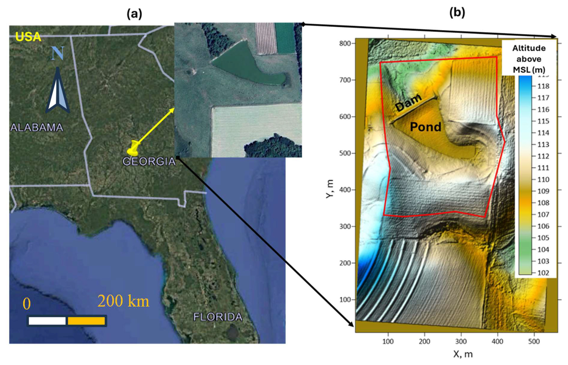
Figure 1 Location: Map data © 2025 Google (a) and land topography of the study area (b). The red line represents the boundary of the simulation domain.

Soil cover at the site consists of a loamy sand (average of 85 % sand, 9 % silt, and 7 % clay) to depths of 60–80 cm, underlain by sandy clay loam (average of 62 % sand, 8 % silt, and 30 % clay) containing plinthite, a low permeability layer of hard iron-rich soil restricting hydraulic connectivity between surface and groundwater (Blume et al., 1987). The latter soil was used to build the bottom of the pond and the dam.

Weather conditions were monitored by the USDA-ARS Southeast Watershed Research Laboratory (SEWRL) at the site to measure air temperature and humidity, wind speed, solar radiation, and soil and water temperature. Data were collected from a climate station located at the SCF noted as “Rain Gage 80” in the SEWRL public data website (https://radio.tiftonars.org/rg80.htm, last access: 5 May 2026). Specifications for instrumentation follow the configurations for the Little River Experimental Watershed climate stations described in Bosch et al. (2007).

2.2 Quantifying pond use and bacterial concentrations in cattle manure

Cattle use of the pond and the pasture area draining into the pond was evaluated using automated trail cameras. Eight cameras were fixed to solid structures (e.g., fence posts, trees) and their fields of view (FOVs) captured overlapping images of the pond at regular intervals. Three comparable camera models were used for the study, including 3 Bushnell 24MP Prime Low Glow (Model 119932C), 3 CamPark, and 2 Coleman (Model CHD400W) cameras. Cattle in the pond were imaged from July 2022 to December 2023. Secure digital (SD) removable media cards were used to record the imagery and were replaced every 6 to 10 weeks for the duration of the study. Imagery was downloaded and stored on a file server for subsequent analysis. The imagery was visually assessed for pond use by cattle by a single observer for all days. Images were reviewed from each camera, and the number of cows in the pond was counted in each image. Tallied viewpoint counts were summed according to the model finite element mesh (FEM) nodes segmentation of the shoreline described below, multiplied by the time interval of the camera setting (5 to 30 min), and divided by 1440 min d⁻¹. The resulting values were summed for each shoreline segment to produce a daily value of “cow days” (Cex). To evaluate the accuracy of the visual assessment, two additional independent observers conducted validation counts of a sample of the imagery following the same protocol, and agreement among the three observers (OBS1, OBS2, and OBS3) was evaluated.

Between February and May 2023, 18 fresh cow manure samples were collected from the area around the pond. Samples were collected into 50 mL conical tubes using a sterilized tongue depressor and were then placed on ice for storage and transport to the laboratory. Laboratory processing of manure samples occurred within 24 h of sample collection. Briefly, 2 g of manure was blended with 200 mL of sterile, deionized water for 2 min on the highest setting. Mixed samples were then allowed to settle for 15 min before aliquots were used to prepare serial dilutions of the manure mixture. Diluted manure solutions were processed in duplicate using the Colilert method (IDEXX, Westbrook, Maine), which produced a most-probable-number (MPN) of E. coli in each sample. An MPN was then calculated per mass of manure (MPN E. coli kg⁻¹) using information from a dry weight analysis of the manure.

2.3 Water sampling

Figure 2 shows the locations of the water sampling points for measurements of E. coli concentration and of the camera viewpoints for monitoring cattle. For the water sampling points, locations with even numbers (2, 4, 6, 8, 10, 12, 14, 16, not shown) have coordinates the same as locations with odd numbers (1, 3, 5, 7, 9, 11, 13, and 15), respectively. However, locations with odd numbers were sampled at the pond surface, whereas locations with even numbers were sampled at a depth of 50 cm using a peristaltic pump. Locations 17 to 26 were sampled at the surface near the banks. All samples were taken between 10:00 and 12:00 EST in the absence of cows.

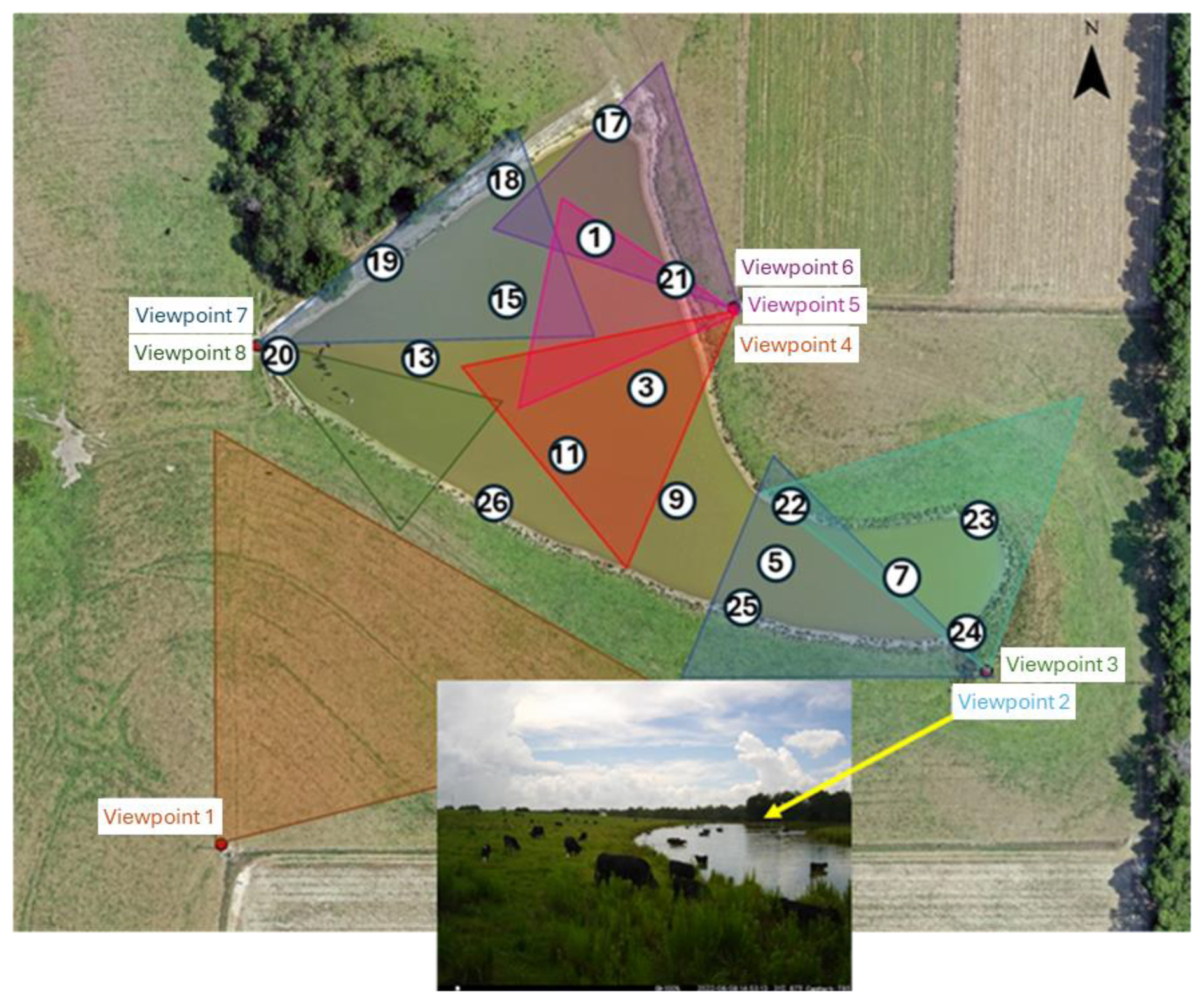
Figure 2 Locations of water sampling points (1–26) and cattle monitoring cameras (Viewpoints 1–8). The insert shows an example of an image taken at monitoring viewpoint 2. Orthoimage from 7 July 2022 by USDA-ARS, Southeast Watershed Research Laboratory, Remote Sensing and Mapping Group, Tifton, Georgia, USA. The imagery was collected with a Hasselblad L1d-20C 20mp camera using a DJI Mavic 2 Pro L1P drone, and created using Pix4D Mapper image processing software.

2.4 Mathematical model

Accounting for the complexity of hydrogeological and hydrochemical processes, we choose the HGS (Therrien et al., 2010) as a basis for the model. In HGS, the flow of water is simulated in a fully integrated mode; water derived from rainfall inputs is partitioned into components such as overland and stream flow, evaporation, infiltration, recharge, and subsurface discharge into surface water features such as lakes, streams, and wetlands in a natural, physics-based fashion. It employs a fully coupled numerical approach, allowing the simultaneous solution of both the surface and variably saturated subsurface flow, solute transport, and heat transfer.

The mathematical model of the watershed flow and transport comprises the following components. The Richards equation simulates three-dimensional transient subsurface flow in a variably saturated porous medium (PM domain). The van Genuchten (1980) relations are used to calculate the pressure-saturation relationship and hydraulic conductivity. The two-dimensional depth-averaged diffusive wave equation describes overland water flow (OVL domain). The subsurface and surface flow equations are fully coupled. Evapotranspiration affects surface and subsurface flow domains and is modeled as a combination of transpiration from vegetation and evaporation. Microbial transport is described by 3D and 2D coupled advection-dispersion equations in the subsurface and surface, respectively. We chose the linear Henry isotherm for simulating E. coli sorption. A first-order decay reaction describes the bacteria's die-off. The present model does not explicitly simulate soil and manure erosion, suspended sediment transport, settling, or resuspension. As a result, bacterial transport is represented primarily through direct runoff and overland flow pathways, without accounting for attachment to or release from suspended or bed sediments. However, the model accounts for the release of bacteria from cowpats uploaded onto the soil surface.

The numerical solution of partial differential equations and the initial and boundary conditions are done by the control volume finite element approach.

2.4.1 Finite element mesh

The numerical setup of the simulation domain is shown in Fig. 3. The lateral boundary was chosen to cover most of the area where runoff water flows towards the pond. The 2D triangular finite element mesh (FEM) was created using AlgoMesh software (https://www.hydroalgorithmics.com/software/algomesh, last access: 5 May 2026) (Fig. 3a). It consists of 2882 nodes and 5595 triangular elements. The mesh has the highest density of nodes and elements near the pond boundary.

The base of the simulated profile is located at a depth corresponding to an altitude of 100 m. The thickness between the base and soil surface was divided into three layers (U1–U3, Fig. 3b), and each layer was split into 2 to 4 sublayers. The floors of the layers U2 and U1 are located at depths of 0.1 and 1.0 below the land surface, respectively, thus mimicking the surface topography. In the model, each sublayer is considered an independent layer defining the height of triangular prisms, which presents the vertical extension of the 2D plane mesh within each layer (Fig. 3c).

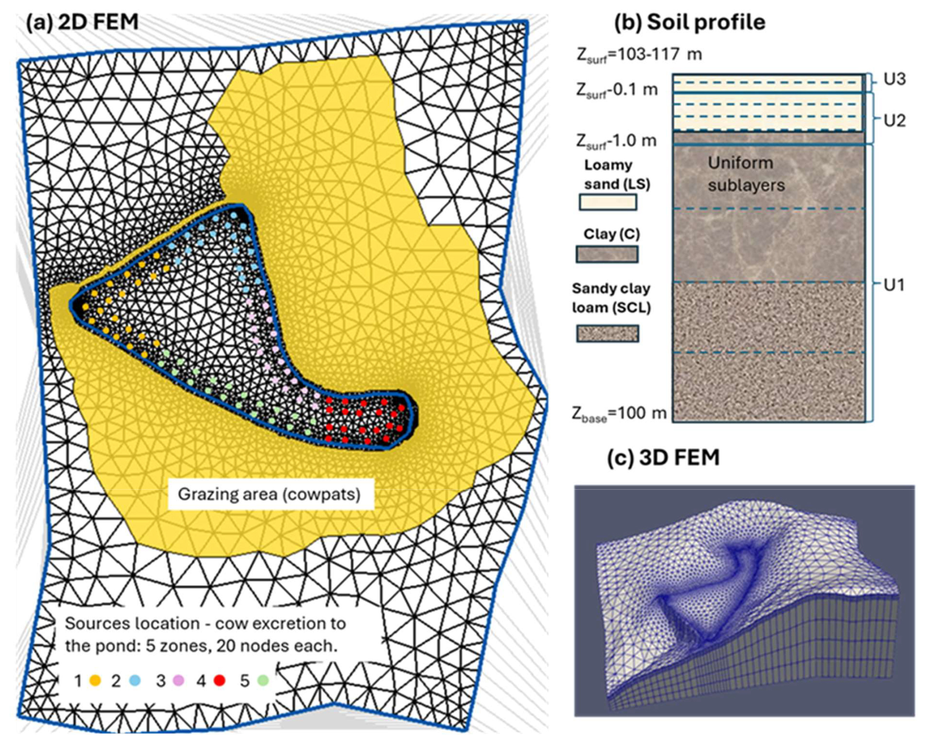
Figure 3 Numerical model setup: (a) The 2D triangular finite element mesh in the simulation domain. Cowpats (a flat, round piece of cow dung) are located in the yellow color area. Colored circles represent the location of sources to simulate cattle excretion in the pond. (b) Schematic representation of numerical mesh layers in the simulated profile. Solid and dashed horizontal lines represent the boundaries between layers and sublayers, respectively. (c) 3D finite element mesh (FEM).

2.4.2 Initial conditions

Initial conditions were obtained by running multi-year simulations. For the subsurface flow, a constant pressure head of −2 m in each node of the finite element mesh was used. For the surface domain, the initial water depth was 10⁻⁷ m in each node, i.e., the pond was assumed to be empty. These initial conditions were corrected during simulations: (1) For two years, a constant precipitation rate (flux at the soil surface of 0.01 m d⁻¹) was simulated to “fill in” the pond with water and establish a steady-state flow regime in the simulation domain; (2) the resulting distribution of heads was taken as a new initial condition and the model was run with varying precipitation and evapotranspiration for 6 years to establish a quasi-stationary flow regime; (3) Finally, the initial conditions were taken from the results obtained at the end of the simulations.

Initially, the prescribed concentration of bacteria was equal to 0 everywhere in the domain. Then, during multi-year simulations, a concentration distribution was developed in the simulation domain, exhibiting cyclic behavior with time, and it was accepted as the initial condition for 1 January 2022.

2.4.3 Boundary conditions and internal source terms

In the study area, the groundwater level of a regional artesian aquifer was detected at around 70 m above mean sea level (m a.m.s.l.) (Watson, 1976), which is 30 m below the bottom (100 m) of the simulated domain. Therefore, the groundwater is not included in simulations. The free drainage boundary condition at the bottom and no flux at the lateral boundaries were prescribed.

At the soil surface, time-variable precipitation rate and evapotranspiration were prescribed. The latter is calculated from the potential evapotranspiration, computed using the Penman-Monteith equation (Monteith, 1965; Danielescu, 2022).

The critical depth boundary condition at the watershed boundary was set to the surface flow domain. The rainfall and evaporation rates are prescribed as volumetric flow fluxes per unit area.

For the bacteria transport, zero-gradient and zero-concentration conditions were set in the subsurface domain along the inflow and outflow lateral boundaries, respectively. The third-type (Cauchy) boundary condition was set at the surface, expressing the balance between bacteria's advective flux at the soil surface and their advective and dispersive fluxes below. The land surface is divided into a grazing area with cowpats and the rest (Fig. 3a). Cowpats were assumed to be uniformly distributed over the grazing area. The boundary concentration (and mass flux) equals zero in the area free from cowpats. For the grazing area, a sub-model was developed to calculate the boundary concentration of bacteria. The sub-model simulates the daily evolution of concentration depending on the load of cowpats and the initial concentration of bacteria (see Appendix A for the equations). On each specific day, the fate of bacteria concentration in cowpats that were loaded during that, and every previous day was calculated using the Q₁₀ model (Martinez et al., 2013). The latter computes the bacteria's die-off/survival rate depending on weather conditions. The concentrations of released microorganisms are calculated as a function of precipitation according to Bradford and Schijven's (2002) equations for each cowpat's load, accounting for the remaining mass of bacteria during the current day. The resulting boundary concentration is assessed as a sum of those concentrations.

Cattle excretion to the pond was simulated by introducing the internal source terms in the FEM nodes (Fig. 3a). The nearshore pond area, where bathing cattle were observed, was divided into five zones. Each zone includes twenty FEM nodes. These nodes do not coincide with the water sampling locations. The source rates were calculated from the number of cattle and the time they spent in the pond (Sect. 3.1). The time-variable boundary conditions and source/sink terms were prescribed on a daily scale.

2.5 Model parameters

We adopted the values of model parameters from different sources or estimated based on existing experimental data or during simulations. Tables 1 and 2 present parameter values used in the simulations.

Table 1 The model parameter values for the subsurface domain.

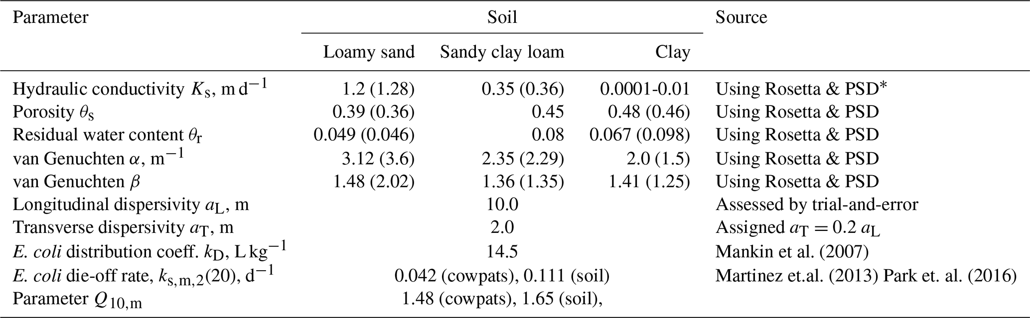
^* PSD – particle size distribution.

The geology of the subsurface is not well known. The following composition of soil layers was accepted, based on available information: loamy sand to a depth of 0.5 m, below which a clay layer of variable thickness extends down to the upper half of layer U1 (Fig. 3b). The lower half of U1 is presented by sandy clay loam. The pond bottom (to 0.5 m depth) and the dam are built from clay with the hydraulic conductivity of 0.0002 m d⁻¹.

Table 2 The model parameter values for the surface and evapotranspiration domains.

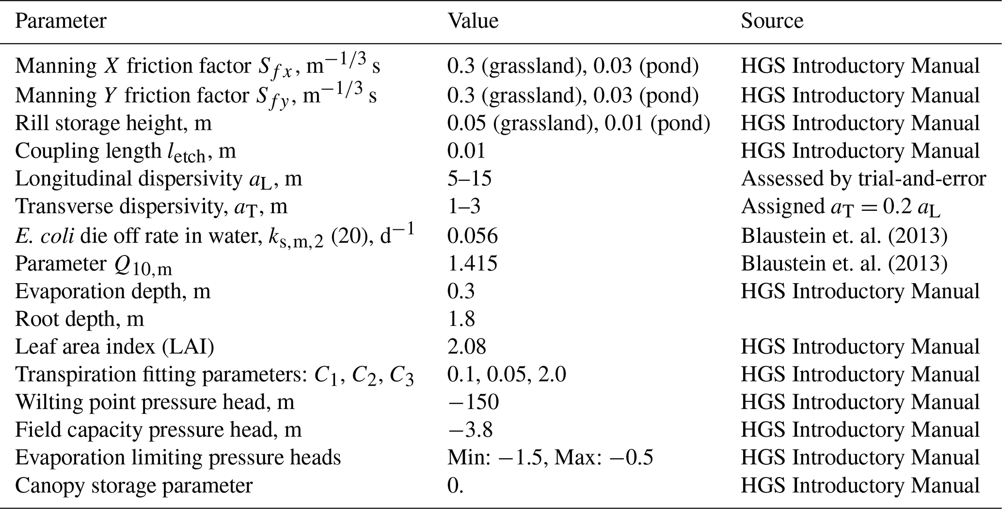
E. coli fate and transport simulations were performed for 2022–2023. To progress the numerical convergence and reduce simulation time, we use relative concentrations $C_{\mathrm{r}}=C/C_{\max }$, where $C_{\max }=\mathrm{1.4}\cdot {\mathrm{10}}^{\mathrm{10}}$ MPN m⁻³ is the maximum value of boundary concentration at the soil surface. The value of the longitudinal dispersivity values for the porous media domain was chosen to be 10 m, considering the scale problem (Neuman, 1990). There is no data concerning longitudinal dispersivity for the overland flow domain. Therefore, we tested a few values of this parameter from 5 to 15 m. Longitudinal dispersivity equal to 12.5 m produced a better agreement between simulated and observed concentrations. The transverse dispersivities were $\mathrm{1}/\mathrm{5}$ of the longitudinal ones for porous media and overland flow domains.

E. coli die-off/inactivation rates exhibit considerable variability depending on environmental conditions, e.g., temperature, moisture, pH, organic matter content, attachment to particles, solar radiation, predation, and matrix type such as manure, soil, runoff, or pond water (Lim and Flint, 1989; Soupir, 2007; Ravva and Korn, 2007; Muirhead and Littlejohn, 2009; Oliver et al., 2006; Tran et al., 2020). The E. coli die-off parameters in Tables 1 and 2 were taken as average over the parameters for datasets presented in published databases. The Q₁₀ model parameters of E. coli survival in water were averages over 16 survivals in wastewater datasets presented in the work of Blaustein et al. (2013), and the Q₁₀ model parameters of E. coli survival in manure were averages over seven experimental datasets with bovine manure published by Martinez et al. (2013).The E. coli temperature-dependent die-off in manure, soil, and water was simulated. The current version of HGS does not allow the die-off rate in the surface flow domain to be prescribed as a function of temperature. Therefore, this parameter (Tables 1 and 2) was recalculated for each three-month-long season using mean temperature values and used piecewise by restarting simulations for each time interval.

3 Results and discussion

3.1 E. coli boundary conditions and internal source terms

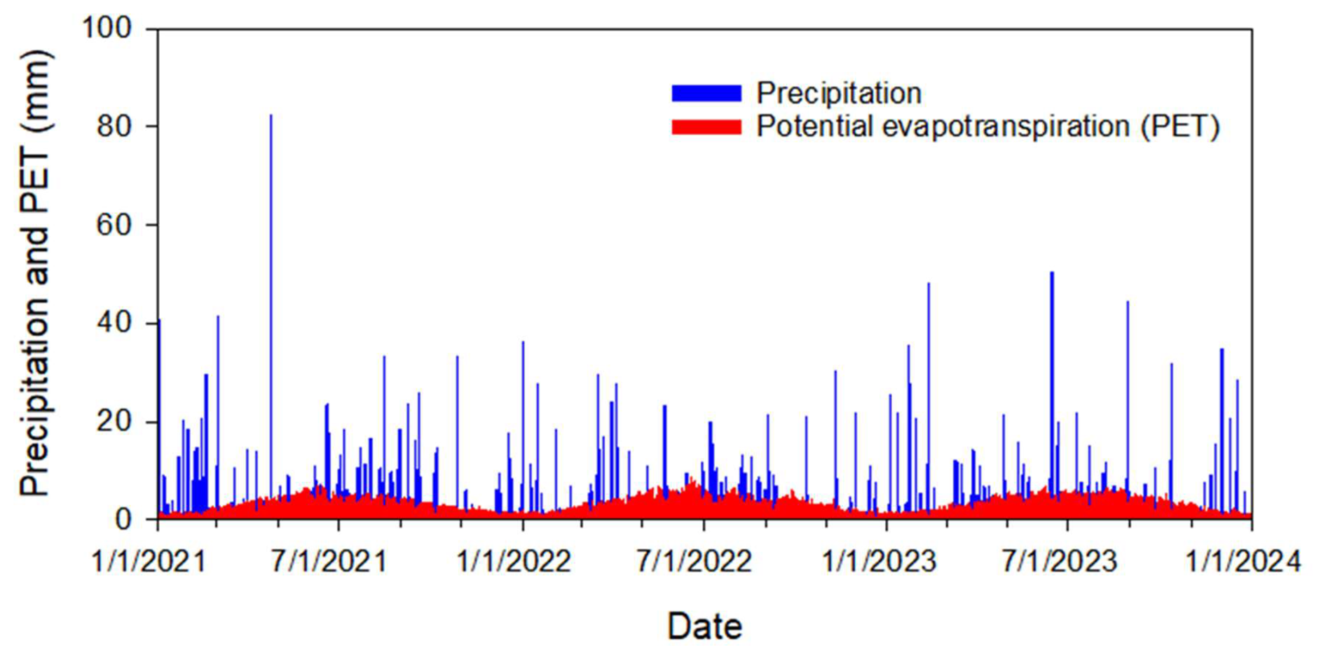
All simulations were carried out using available weather data for a time interval from 1 January 2021, to 31 December 2023. Annual precipitation was 1375, 998, and 1167 mm in 2021, 2022, and 2023, respectively. Figure 4 shows rainfall and calculated potential evapotranspiration in the study area in 2021–2023.

Figure 4 Precipitation and calculated potential evapotranspiration.

The surface Cauchy-type boundary concentration at the grazing area (Fig. 3a) was calculated using the equations presented in Appendix A, as described above in Sect. 2.3.3. We assume that 50 cattle (the maximum number of animals that appeared in monitoring camera photos) were grazing in the watershed. The total grassland area of around 60 000 m² was estimated based on recent aerial imagery provided in Google Earth (version Pro 7.3). Nennich et al. (2005) estimated the average daily load of manure of 38.6 and 66.3 kg d⁻¹ per cow for dry and lactating cows, respectively. The ratio of urine to feces in dairy cows varies, but on average, slightly less than one-third of manure is urine. Thus, we estimate average daily feces excretion as $\mathrm{0.5}\times (\mathrm{38.6}+\mathrm{66.3})\times \mathrm{0.667}=\mathrm{35}$ kg d⁻¹ per cow. Monitoring shows that during the day, cows usually graze for at least 12 h. Therefore, we estimate solid manure load M₀= kg d⁻¹ per cow × 12 h$/$24 h × 50 cows$/$60 000 m² = 0.0146 kg m⁻². The initial concentration of E. coli in fresh cowpats, $m_{i\mathrm{0}}=\mathrm{7.38}\cdot {\mathrm{10}}^{\mathrm{8}}$ MPN kg⁻¹, was calculated as an average in 16 samples collected in 2023. Other parameters in Eqs. (A3)–(A4) were α_m=23.375 h⁻¹, β_m=1.732, and E_r=1 (Stocker et al., 2018). No cattle were observed in the field from the beginning of December to the end of February. Figure 5 shows the calculated boundary concentrations.

Figure 5 Simulated temporal variation of E. coli surface boundary concentration at the grazing land.

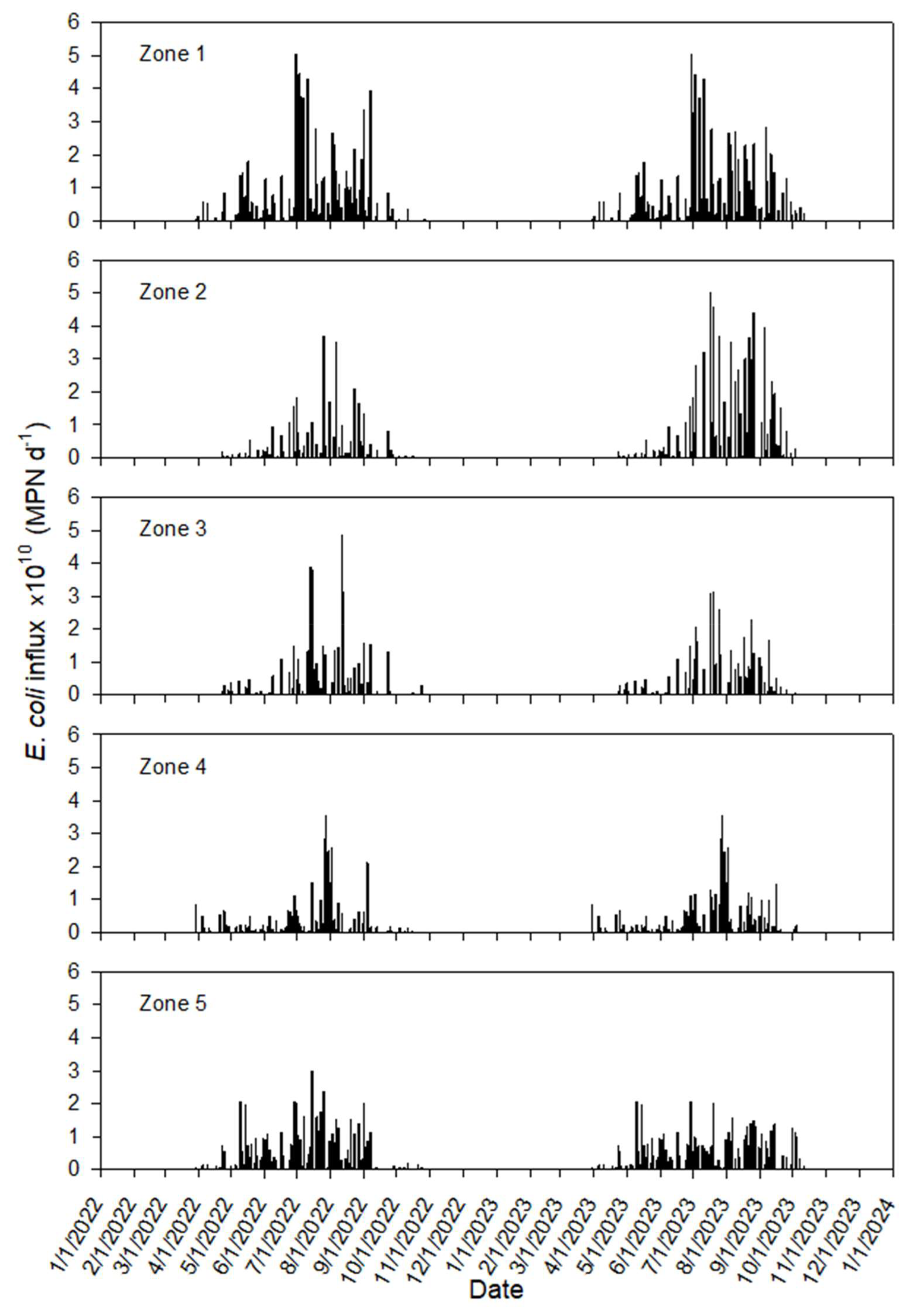
The influx of source terms representing E. coli loading from direct cattle excretion into the pond was calculated as described in Sect. 2.4.3. Validation of the visual assessment of trail camera imagery to derive Cex yielded strong correlations among the three independent observers (OBS1 v OBS2, n=64, R²=0.93; OBS1 v OBS3, n=46, R²=0.90; OBS2 v OBS3, n=18, R²=0.99). It was assumed that all bacteria were immediately released from manure in the pond. Accounting for the daily cow excretion (as explained above for the surface boundary concentration) and E. coli concentration in cowpats, we calculated the daily source rate for each pond zone (Fig. 6) as a portion of the daily manure excretion. The rate for each node is one-tenth of the zone rate. Cattle use monitoring started in July 2022. Therefore, in simulations for the period January–June 2022, where there were no observations, the calculated rates for 2023 were used.

Figure 6 Calculated E. coli inputs to the pond through cattle excretion for the five zones.

3.2 Flow simulation results

Water flow simulations were carried out for 2021–2023. The simulated water level in the pond is controlled by a balance of inflows (precipitation and overland runoff) and outflows (evaporation, infiltration through the pond bottom and dam). To ensure realistic pond persistence during the multi-year simulation period, while preventing unrealistic complete drying while avoiding excessive overflow, we fitted the hydraulic conductivity of the clay liner at the pond bottom to a value of 0.0002 m d⁻¹. Increasing this parameter above 0.0002 m d⁻¹ resulted in excessive seepage losses, leading to a significant and unrealistic decline in the simulated pond water level over the simulation period, which was inconsistent with observed or expected pond behaviour in the study area.

The rest of the parameters are presented in Table 1. During periods with high precipitation, perched water was developed above the clay layer (around 0.5 m below the land surface, not shown). Daniels et al. (1978) reported that soil horizons having 10 % of platy plinthite will perch water.

Runoff is rarely observed in the area. The HGS model calculates fluid fluxes across the pond boundary. Water fluxes are computed between active nodes (located on the pond boundary – dark blue dots in Fig. 3a) and contributing nodes (located just outside the pond boundary). The calculated surface water flux represents the simulated runoff to the pond (Fig. 7).

Figure 7 Computed runoff to the pond.

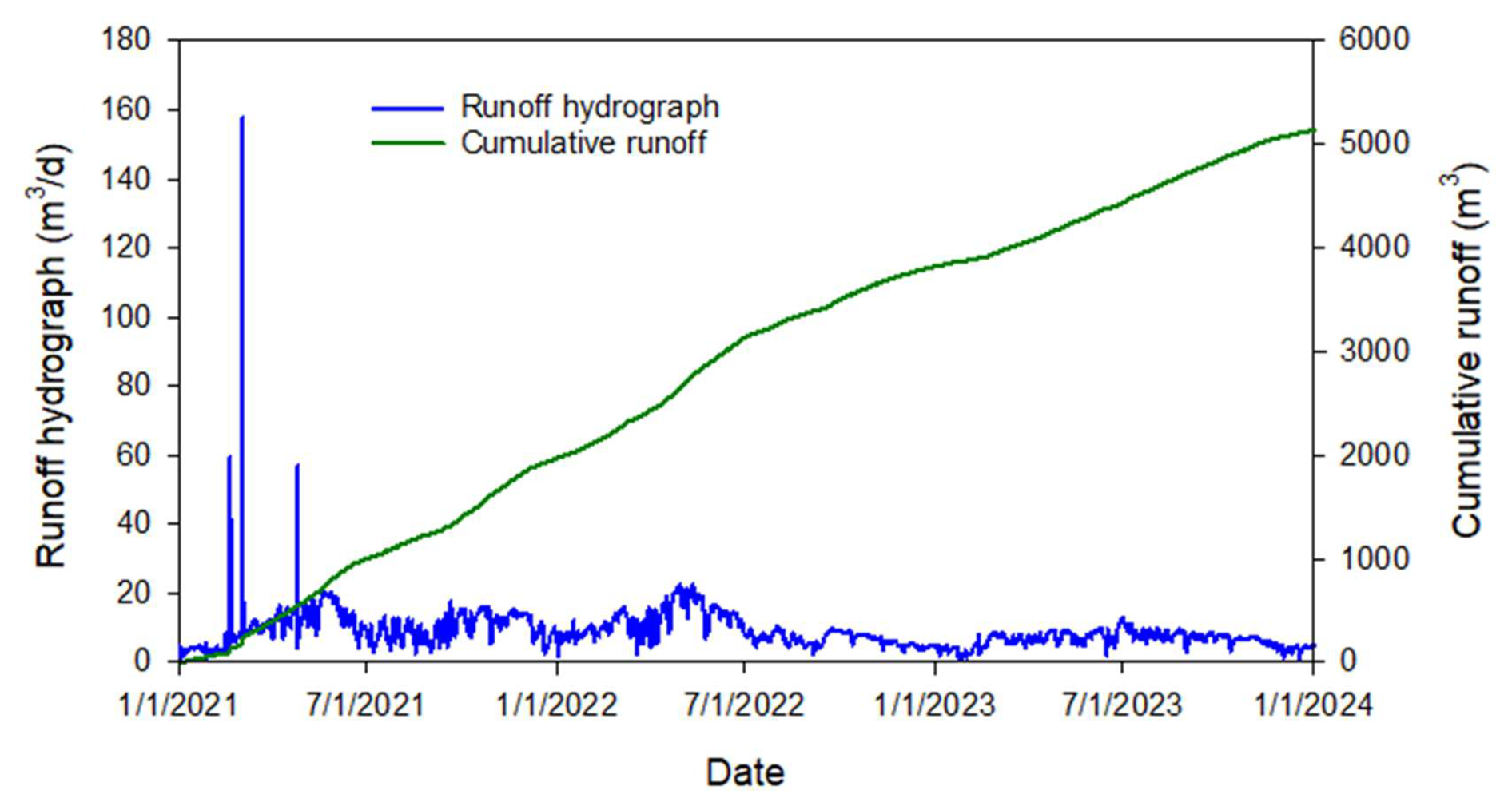
At the beginning of 2021, three significant flow events occurred after intensive 30, 50, and 82 mm rainfalls on 18 February, 1–2 March, and 24 April, respectively. During the rest of the time, the average computed surface flow rate to the pond is around 4.4 m³ d⁻¹. The latter is a relatively small value given a 650 m-long pond perimeter. This small but persistent surface water inflow to the pond during dry periods (no precipitation), attributable to slow drainage of shallow subsurface lateral flow (interflow or return flow) from upslope areas that reaches the pond via surface pathways. This is distinct from precipitation-driven overland flow/surface runoff, which occurs only during or immediately following rainfall events (Tarboton, 2003).

Simulated changes to pond water volume (m³) and water level (m a.m.s.l.) were tracked over the study period (Fig. 8). The simulated minimal and maximal water levels were 109.03 and 109.37 m a.m.s.l. A rise in water level by 0.34 m causes an increase in water volume from 10 770 to 16 075 m³.

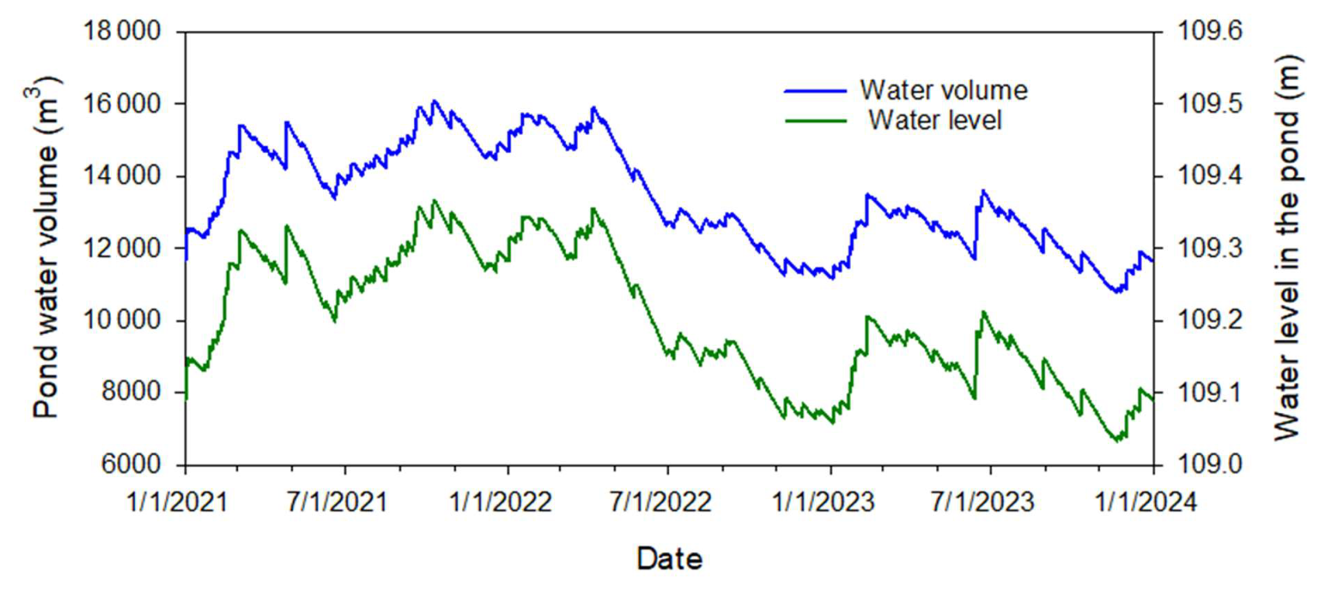
Figure 8 Simulated temporal variation of water volume and level in the pond (above mean sea level).

3.3 Bacteria fate and transport simulations

3.3.1 Results for individual locations

Observed and simulated E. coli concentrations in the interior and nearshore pond sampling locations were compared for each sample location (Figs. 9 and 10). The non-calibrated model tolerably mimicked E. coli concentration patterns and times of peak events in many of the pond's sampling locations. Concentrations increased during summer and decreased during winter months.

For the internal sampling locations 1 to 15, correlation coefficients between the monitored and simulated E. coli concentrations varied between 0.24 and 0.44. An exception was location 7, where the correlation coefficient was −0.01. For the near-shore sampling locations 17 to 26, the correlation coefficient varied between −0.15 and 0.32.

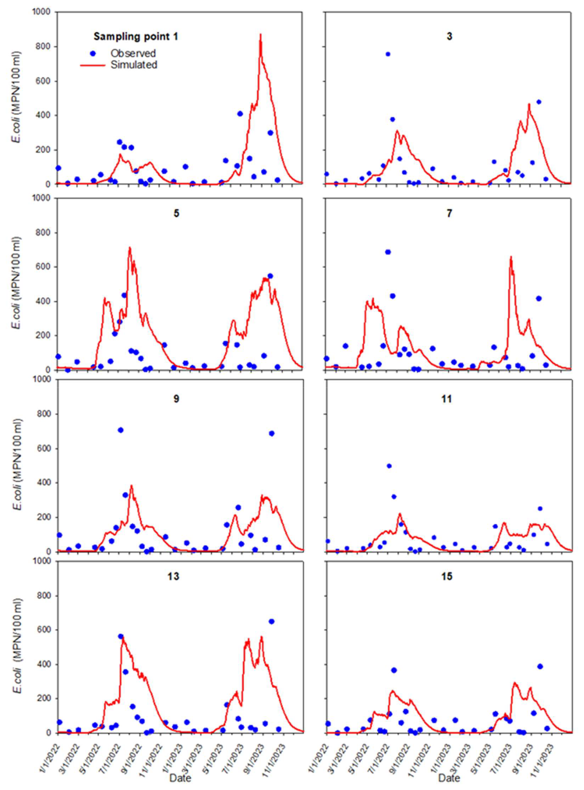
Figure 9 Observed (blue dots) and simulated (red line) E. coli concentrations at interior sampling locations 1–15.

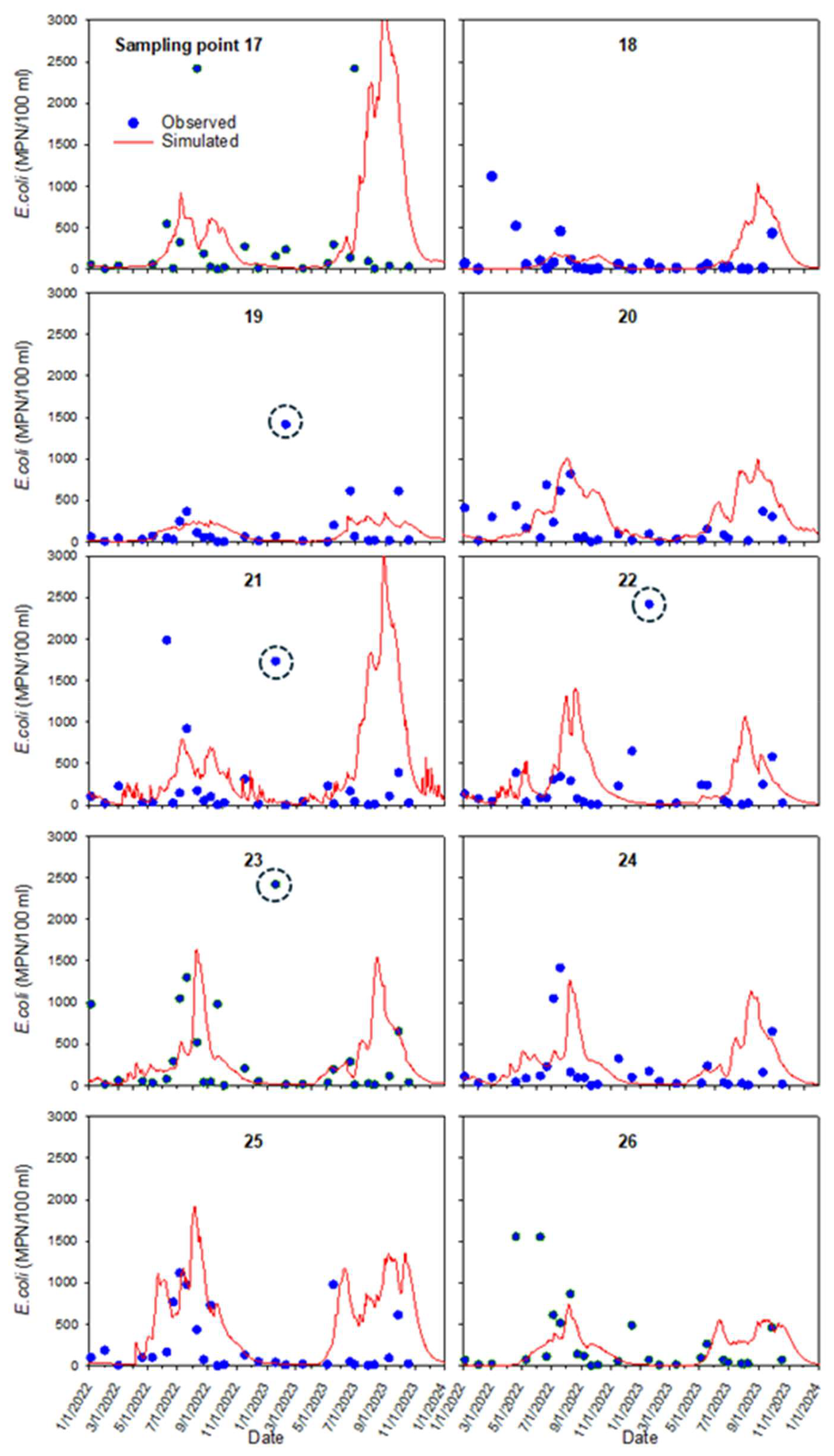
Figure 10 Observed (blue dots) and simulated (red line) E. coli concentrations at nearshore sampling locations 17–26. Dashed circles indicate winter increases in concentrations on 18 January 2023.

The observed differences between simulated and measured concentrations in individual sampling locations might originate from the model setup and computational features. The simulated concentration peaks strongly depended on the proximity of the sampling points to the internal source locations, which were constant in time. Cattle frequently moved across the pond in different directions, which affected the concentration distribution. Most assigned locations for the pond's internal source were 10–20 m from the nearest sampling point.

The reproduction of mixing in the pond might be locally unsatisfactory. Figure 11 shows the simulated relative E. coli concentration distribution at the surface for different dates. Concentration in the source locations, simulating cattle excretion in the pond (Fig. 3a), rises during summer and dissipates in the winter. Simulations show a low E. coli concentration zone in the middle of the pond during the entire simulation period. For example, the model underpredicts peak concentration at sampling location 15 (Fig. 9) in summer 2022 and autumn 2023. This indicates that mixing in the pond was stronger than the dispersion mechanism suggests. Lateral transport is often dependent on persistent wind-forced circulation. Henderson et al. (2024) describe wind-forced processes responsible for ponds' vertical mixing or lateral transport. Additional mixing resulting from induced eddies may cause more rapid cross-pond mixing and potentially affect pond ecology and biogeochemistry. At sampling location 23, the increase in concentration could be due to the occasional resuspension of bacteria from the bottom sediments during sampling.

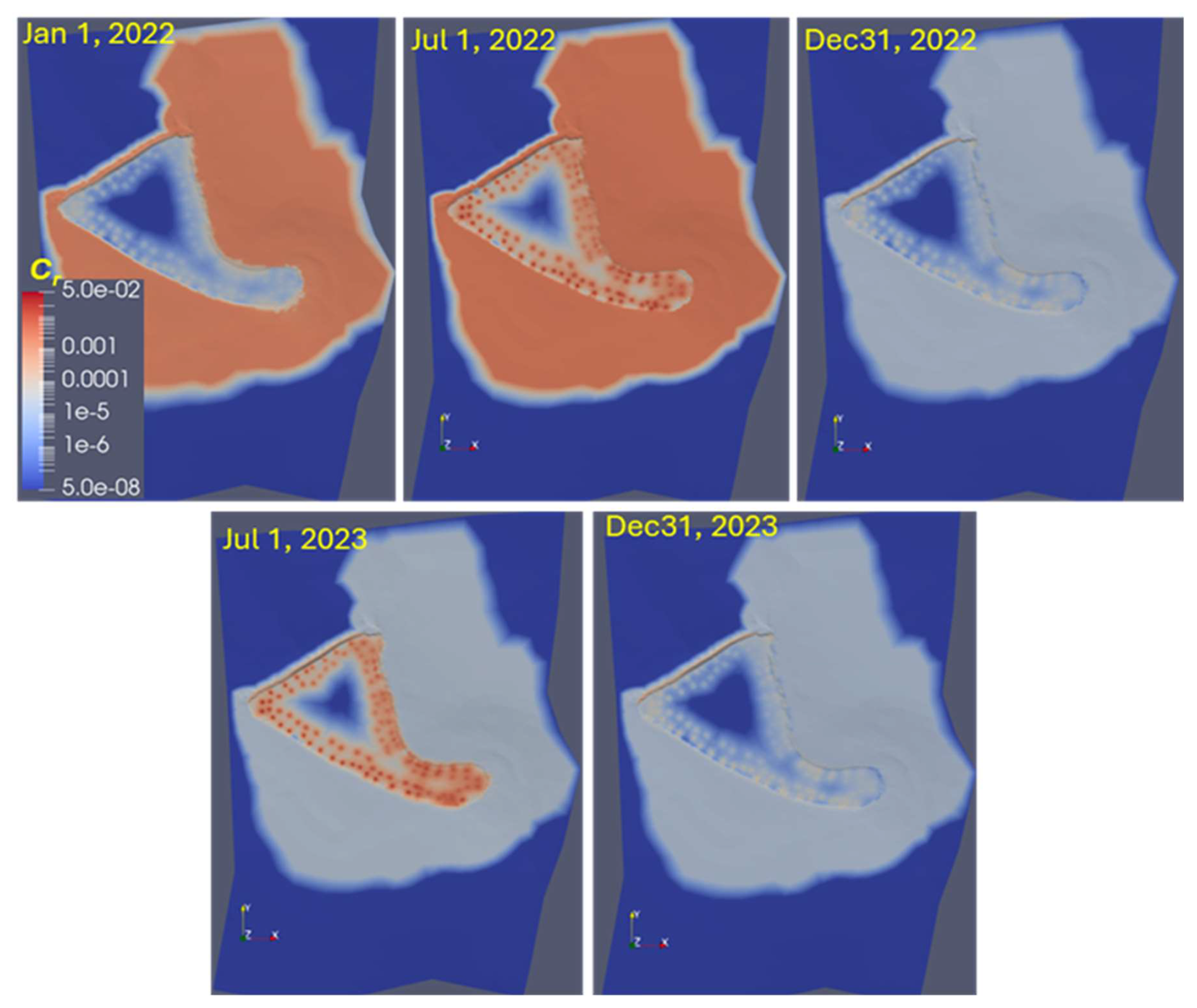
Figure 11 Simulated spatiotemporal distribution of the relative E. coli concentration at the surface. $C_{\mathrm{r}}=C/C_{\max }$, $C_{\max }=\mathrm{1.4}\cdot {\mathrm{10}}^{\mathrm{10}}$ MPN m⁻³, the legend is on a log scale.

More insight could be expected from considering the specifics of E. coli survival in waters rich in organic matter and nutrients (Cho et al., 2021). Blaustein et al. (2013) analyzed the database on E. coli survival in various surface waters. They found that the logarithm of E. coli remained approximately constant or even grew for some lag period time after the inactivation experiments in wastewaters with high content of organic matter and nutrients. After the lag period. The dependence of log C on time changed to a linear decrease. No model has been proposed to estimate the duration of the lag period in wastewater so far.

A sudden rise in E. coli concentration was observed on 18 January 2023, at sampling locations 19, 21, 22, and 23 (Fig. 9, dashed circles). The model does not reproduce this increase. The monitoring camera photos show flocks of birds in the pond near the first three locations 1 to 2 days before the sampling date. At the same time, the model's internal sources on that day were equal to zero since there were no cattle in the pond. We hypothesized that excretion by birds was a reason for elevated E. coli concentrations. During the fall and winter, Georgia's inland freshwaters become populated with waterfowl such as ducks, Canada geese, and migratory birds (Balkcom et al., 2025). One duck generates on average 3.8 ⋅ 10¹⁰ E. coli CFU per day (Moriarty et al., 2011), which is similar to the daily E. coli output from one cow (4 ⋅ 10¹⁰ MPN (g wet feces)⁻¹ d⁻¹ in this work). It appears that the contribution of waterfowl can be very substantial in comparison with cattle contributions (see Fig. 5). To our knowledge, the fraction of waterfowl excreta that enters water has not been reported in the literature. Overall, we concur with Vazquez et al. (2021) who emphasized the need to collect more data on the fecal contamination inputs of the ponds.

3.4 Results for the pond as a whole

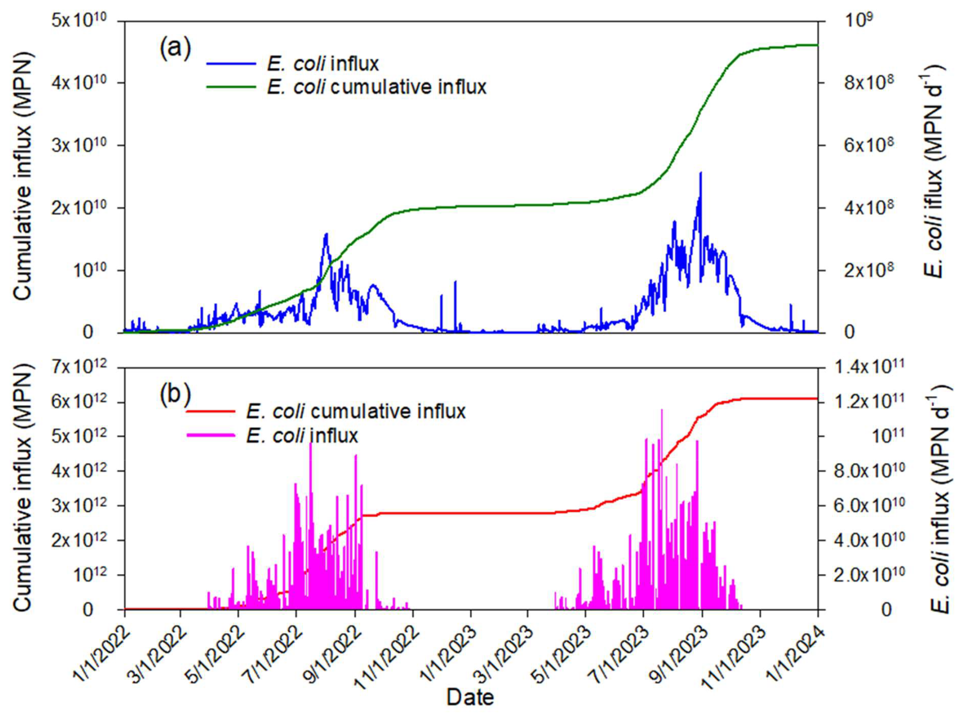
The HGS computed temporal E. coli fluxes entering the pond with surface water. The influxes of E. coli to the pond were visualized along with their calculated cumulative numbers over time for both sources of runoff (Fig. 12a) and direct excretion of feces (Fig. 12b). At the end of simulations, the number of bacteria entering the pond by manure excretion was around 130 times greater than by surface runoff. Simulations show that water flowed mainly from the pond into the subsoil, so that E. coli concentrations in the subsoil did not affect the water quality in the pond.

Figure 12 Simulated E. coli fluxes to the pond: (a) with runoff; (b) excreted into the pond.

Simulated and observed concentrations of E. coli were each averaged over the interior and nearshore sampling locations (Fig. 13). Averaged values of concentrations at the nearshore locations (17–26) were approximately three times higher than the average of concentrations sampled at interior locations (1–15). Elevated nearshore concentrations may be explained by flushing bacteria to the pond during runoff and direct excretion by bathing cattle, which, according to monitoring, spent most of their time grouped close to the shore.

The summary data in Fig. 13 show that the model describes seasonal average concentration patterns relatively well. However, observed concentrations significantly declined during autumn 2022 and 2023 compared to the model simulation. Clear, shallow water can cause deeper penetration of solar radiation. de Brauwere et al. (2014) indicate that the inactivation of bacteria is caused by UV irradiation. To account for the latter, some models add a term to the overall decay parameter due to sunlight (McCorquodale et al., 2004) or use a decay term depending on the intensity of the solar radiation (Kashefipour et al., 2002). The decrease in the nutrients in water in the fall can also be the reason for the reduction of E. coli concentration.

The descriptive statistics of measured and simulated average concentrations were close when computed over the observation period. The minimum and maximum averages across the pond concentrations were 3.56 and 525.1 for observed and 4.08 and 479.4 MPN (100 mL) for simulated data, respectively. The mean logarithms of average concentrations were 1.70 ± 0.47 and 1.99 ± 0.67 for the measured and simulated data, respectively. The correlation coefficient between measured and simulated logarithms of average concentrations was 0.483. This value was significant at a 0.01 significance level and indicated a moderate correlation.

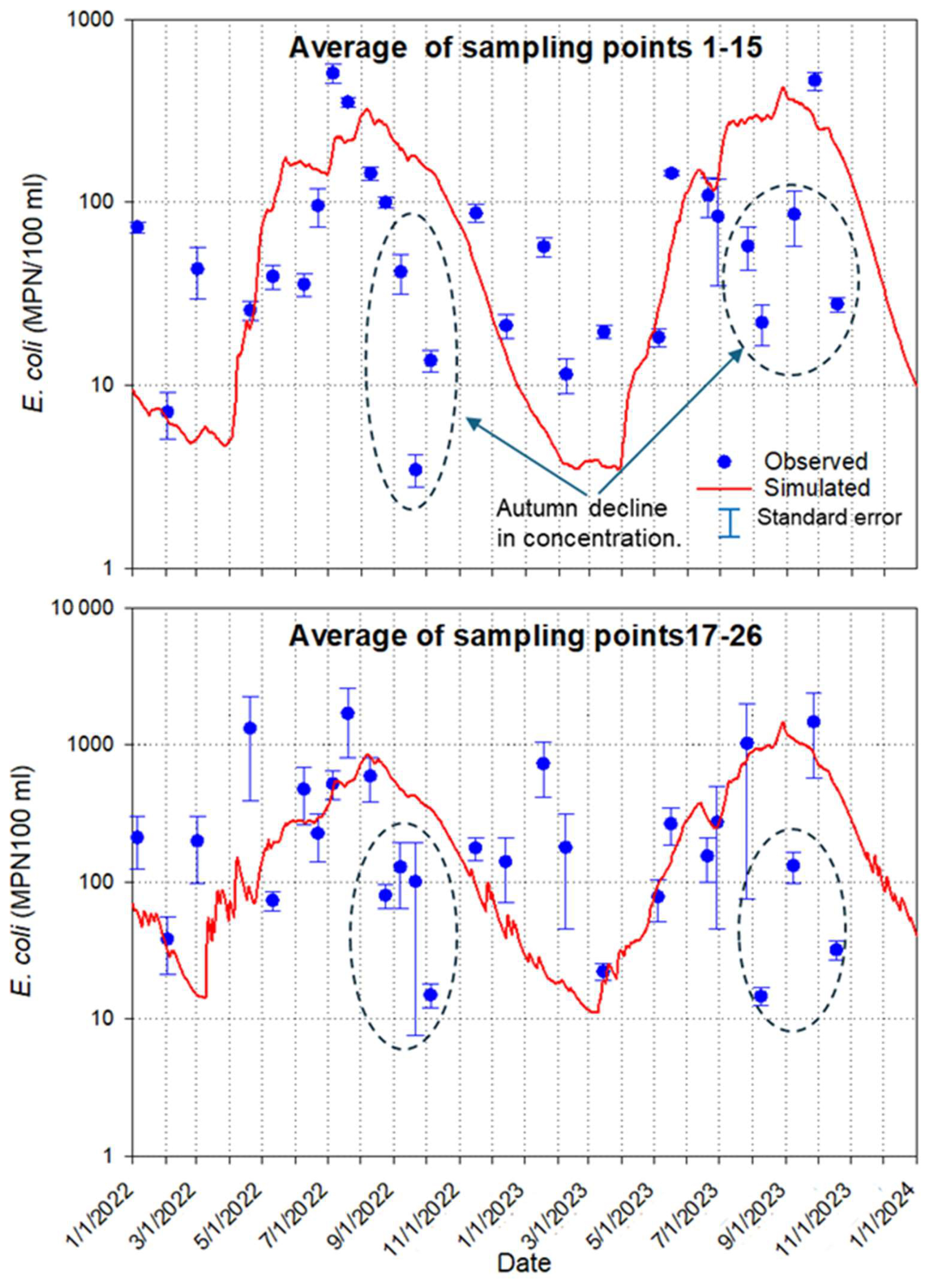
Figure 13 Average E. coli concentrations in the pond's interior (1–15) and nearshore (17–26) sampling locations. Dashed circles indicate an autumn decline in concentration.

4 Discussion

Applying mechanistic fate and transport models relies on model parameter values typically obtained via model calibration. Several factors make the site-specific calibration of microbial fate and transport parameters difficult and sometimes unfeasible. The spatiotemporal variability of microbial concentrations in ponds is very high (Havelaar et al., 2017; Stocker et al., 2022), indicating the need to collect large numbers of samples. The collection and analysis of those samples appear to be unfeasible. That precludes establishing a proper monitoring program for efficient model calibration. The high spatiotemporal variability emphasized the scale mismatch between the water sample size and the water volume, and this sample is used to characterize a much larger water volume used for mass balance computation in the hydrological models.

Flow sub-model parameters have satisfactorily estimated more easily obtainable properties, such as clay or sand content and bulk density (Schaap et al., 2001). Analogous predictive relationships have not been developed, partially because the potential predictors of microorganism survival or release rate have been shown to be dependent on environmental variables that were themselves variable in space and time.

Compendia of microorganism release and survival parameters (Park et al., 2016) show that the parameter values encompass wide numerical ranges and that it is challenging to attribute fate and transport parameter values to specific environmental conditions or management practices. These factors so far substantially limit the applicability of microbial fate and transport modeling. On the other hand, such modeling is in demand due to the need for projections of microbial water quality changes due to environmental changes, adaptation practices, site-specific trade-offs between different water quality aspects, multiple ownership and management along or around irrigation water sources, etc.

In this situation, a relatively important question is: What accuracy can be expected in fate and transport predictions made with average or typical fate and transport parameter values? In other words, given the high spatial variability of microbial concentrations, how significant are the differences between observed and simulated concentrations with average parameter concentrations? The answers to those questions are surprisingly scarce, as the published modeling reports focus on calibration results. These questions have not been researched for agricultural ponds. Results of this work show that if the animal behavior patterns are known, the seasonal trends and magnitudes of pond water microbial pollution can be estimated. Quantifying such patterns for cattle ponds has not been done so far. However, it presents a promising avenue for research.

We realize that the system parameters we have studied are subject to multiple sources of uncertainty. Quantifying this uncertainty and running ensemble simulations with parameters treated as random values presents an interesting avenue for future research. Results of this work, obtained with mean parameter values from various sources, indicate that determining the statistical properties of the bacteria sources can be a first feasible step in that direction.

The present model does not incorporate explicit simulation of soil and manure erosion, suspended sediment transport, settling, or resuspension processes. This omission may underestimate bacterial concentrations in receiving waters during high-flow events, when sediment resuspension, potentially exacerbated by cattle trampling or other disturbances can act as an important secondary source of fecal indicator bacteria. Numerous studies have highlighted the significance of sediment-associated bacterial transport and resuspension in agricultural watersheds (e.g., Jamieson et al., 2005; Pandey et al., 2012; Bradshaw et al., 2021). Future model extensions could benefit from coupling a sediment transport sub-module to more comprehensively capture these interactions.

The current implementation does not include site-specific calibration or formal sensitivity analysis of key parameters (e.g., die-off rates, sorption coefficients as listed in Tables 1 and 2). While these steps would provide valuable insights into parameter influence and model behavior, and are recommended for future applications, the present work prioritizes proof-of-concept integration and qualitative assessment over quantitative optimization. Similarly, the model currently incorporates a single dominant removal process (first-order die-off/inactivation) to maintain simplicity during initial coupling; additional mechanisms (e.g., settling, resuspension, or biotic interactions) were not included but represent promising extensions. Such enhancements could better elucidate ecosystem functioning and inform management strategies to enhance bacterial removal in pond systems, as supported by prior modeling efforts in watershed-scale microbial fate and transport (e.g., Ferguson et al., 2010; Bradford et al., 2013; Cho et al., 2016).

This study contributes to the current state-of-the-art in several ways. First, it applies a fully mechanistic three-dimensional surface–subsurface hydrological model to simulate microbial fate and transport in and around a cattle pond. Unlike many previous studies that rely on simplified or lumped representations of microbial transport, the present approach explicitly resolves hydrological processes controlling bacterial transport through surface runoff and subsurface flow pathways at the watershed scale. Second, the model explicitly accounts for direct microbial loading caused by cattle entering the pond and depositing manure in the water. The magnitude of this source term was estimated from the observed presence of cattle in the pond using time-lapse imagery obtained from multiple trail cameras. To our knowledge, such direct observational quantification of livestock behavior has rarely been incorporated into mechanistic watershed-scale microbial transport models. Third, the study evaluates the ability of a mechanistic model to reproduce observed E. coli dynamics with minimal calibration using primarily literature-based parameter values. This approach addresses a common limitation in agricultural water quality studies, where extensive datasets required for model calibration are rarely available. Finally, the modeling framework provides quantitative insight into the relative importance of different contamination pathways, including surface runoff from manure deposited on pasture and direct microbial loading by cattle entering the pond. The results demonstrate that direct excretion by cattle in the pond can dominate microbial inputs under certain management conditions. Overall, this work demonstrates how mechanistic watershed-scale modeling combined with observational data on livestock behavior can be used to improve understanding and prediction of microbial contamination in agricultural ponds.

5 Conclusions

This study developed the first mechanistic numerical model for bacteria transport from grazing land around a cattle pond. The model was based on the HGS software, simulating fully coupled surface-subsurface flow and transport. The model was tested to simulate E. coli fate and transport in a small pastureland watershed in Georgia, USA, using observations from 2021–2023. The primary goal was to simulate the temporal and spatial distribution of E. coli concentration in the pond. All parameters for this simulation were taken from the literature or estimated from published data. The exception was the rate of E. coli input to the pond from the direct excretion of feces from animals, since such data were not found in the literature. The non-calibrated model could mimic E. coli temporal concentration patterns and peak times reasonably well in most of the pond's sampling locations. There were seasonal differences in correspondence between simulated and measured E. coli time series, and the magnitude of concentration peaks was poorly predicted in some sampling locations. Predictions of the average across-pond concentrations were expected to be moderately accurate. Quantification of microbial inputs for cattle ponds has not been done so far. Still, it presents a promising avenue to estimate the microbial water quality in cow ponds using the data accumulated in past research.

Appendix A: Equations to calculate E. coli concentration released from cowpats at the soil surface (3rd-kind boundary condition concentration)

For day t, the content of microorganism in the applied manure is calculated by (Martinez et al., 2013):

$$\begin{array}{}\text{(A1)}& m_i\left(t\right)=m_i(t-\mathrm{1})e^{-k_{\mathrm{s},\mathrm{m}}}\end{array}$$

Where k_s,m is the rate coefficient which is the function of temperature T at time t, (d⁻¹)

$$\begin{array}{}\text{(A2)}& k_{\mathrm{s},\mathrm{m}}=\left\{\begin{array}{ll}{k}_{\mathrm{s},\mathrm{m},\mathrm{1}},& t\le t_{\mathrm{s},\mathrm{m},\mathrm{1}}\\ k_{\mathrm{s},\mathrm{m},\mathrm{2}}\left(T\right),& t>t_{\mathrm{s},\mathrm{m},\mathrm{1}}\end{array}\right.\end{array}$$

$t_{\mathrm{s},\mathrm{m},\mathrm{1}}$ is the duration of the first stage, d, T is the average daily temperature, °C, and $k_{\mathrm{s},\mathrm{m},\mathrm{1}}$ and $k_{\mathrm{s},\mathrm{m},\mathrm{2}}\left(T\right)$ the survival rates at the first and second survival stages are respectively.

The bacterial population may grow, remain stable, or die off during the first survival stage, and decrease during the second stage of survival. On the second stage, the values of $k_{\mathrm{s},\mathrm{m},\mathrm{2}}\left(T\right)$ can be described with the Q₁₀ model (Martinez et al., 2013).

$$\begin{array}{}\text{(A3)}& k_{\mathrm{s},\mathrm{m},\mathrm{2}}\left(T\right)=k_{\mathrm{s},\mathrm{m},\mathrm{2}}\left(\mathrm{20}\right)Q_{\mathrm{10},\mathrm{m}}^{\frac{T-\mathrm{20}}{\mathrm{10}}}\end{array}$$

where $k_{\mathrm{s},\mathrm{m},\mathrm{2}}\left(\mathrm{20}\right)$ is the survival rate at 20 °C, Q_10,m reflects the sensitivity of $k_{\mathrm{s},\mathrm{m},\mathrm{2}}$ to a temperature that is equal to the change in survival rate occurring as temperature changes by 10 °C.

The concentration of released microorganism C_m is calculated according to Bradford and Schijven (2002) as

$$\begin{array}{}\text{(A4)}& {\displaystyle }{C}_{\mathrm{man}}\left(t\right)={\displaystyle \frac{\mathrm{d}{M}_{\mathrm{man}}}{R\mathrm{d}t}}={\displaystyle \frac{M_{\mathrm{0}}{\mathit{\alpha }}_{\mathrm{m}}}{R}}(\mathrm{1}+{\mathit{\alpha }}_{\mathrm{m}}{\mathit{\beta }}_{\mathrm{m}}t{)}^{-(\mathrm{1}+\mathrm{1}/{\mathit{\beta }}_{\mathrm{m}})}\text{(A5)}& {\displaystyle }{C}_{\mathrm{m}}\left(t\right)=m_i{E}_{\mathrm{r}}{C}_{\mathrm{man}}\left(t\right)\end{array}$$

WhereM_man is the cumulative cowpat mass released into the aqueous phase (g), R is rain intensity, cm h⁻¹, α_m (h⁻¹) and β_m are fitting parameters defining the shape of the release curve, and M₀ is the initial mass of cowpats (g cm⁻²), C_man is the aqueous manure concentration (g cm⁻³), m_i is content of microorganism in the cowpats (CFU g⁻¹), E_r is microorganism release efficiency.