Symbolic regression-based regionalization of baseflow separation parameter using catchment-scale characteristics

Accurate separation of baseflow from streamflow is of utmost importance for understanding catchment hydrological processes and supporting effective water resource management. The Smooth Minima Method is a common baseflow separation technique with a segment length parameter (N) representing the catchment average flow event duration. N is usually predicted by a power function with catchment area or defaults to 5 d. Yet these estimations are insufficient given the multivariate nature of N with other catchment attributes. In this study, we employ symbolic regression (SR) to search for possible formulation of N with a range of catchment attributes based on 855 catchments across the Contiguous United States. We ultimately identify three mathematical expressions of increasing complexity, achieving R² values of 0.48, 0.52, and 0.55, compared to 0.23 and −0.84 for the power function and constant values. The three expressions reveal that N increases following a power-law relationship with catchment area (A) and catchment-averaged soil saturated hydraulic conductivity (K_sat) with decreasing rates, while it increases linearly with snow day fraction (f_SWE). The effects of K_sat and f_SWE on N are particularly pronounced for larger values (K_sat > 25 mm h⁻¹ and f_SWE > 0.4) and smaller area (A < 100 km²). The different calculations of N are also evaluated in baseflow separation, revealing higher medians of Kling-Gupta Efficiency of at least 0.84, outperforming the literature-suggested formulas for a maximum increment of 0.22. This study highlights the potential of SR for uncovering physically meaningful formulas in optimal baseflow separation.

1 Introduction

Baseflow is an essential component of streamflow, primarily originating from groundwater, deep interflow, snow melting, and other delayed sources (Xie et al., 2020; Wang et al., 2022; Stoelzle et al., 2020). The proportion of baseflow in streamflow reflects the complex interactions between surface water and groundwater systems (Pelletier and Andréassian, 2020; Xie et al., 2024), and understanding this proportion can aid in water resources management and riverine ecosystem conservation (Yan et al., 2023; Tan et al., 2020). Baseflow is difficult to measure directly and it is usually estimated using baseflow separation methods (Humphrey et al., 2022; Stewart, 2015), which take continuous streamflow data as the only inputs. The performance of baseflow separation is sensitive to parameters of the separation methods, which, if not optimized, may lead to unrealistic baseflow dynamics (Mei et al., 2024b). Incorporating environmental tracer data for parameter optimization is a common practice, as it ensures reliable baseflow separation by maintaining dual mass balance for both tracer concentration and streamflow volume (Cartwright, 2022; Hagedorn, 2020; McMahon and Nathan, 2021). Commonly used tracers include specific electrical conductivity (SEC), turbidity, and stable isotopes, among which SEC is the most widely applied due to its routine availability in many monitoring programs (Mei et al., 2024b). However, a critical challenge arises as this method is not applicable for catchments without continuous tracer data, which unfortunately constitutes the majority of gaged catchments worldwide (Thorslund and van Vliet, 2020; Hou et al., 2024). This limitation hinders accurate quantification of baseflow in most global catchments, despite their long-term streamflow data.

To optimize baseflow separation for gaged catchments lacking continuous environmental tracer data, a viable approach is to transfer optimized parameters from other catchments (Klotz et al., 2017; Feigl et al., 2020). Specifically, prediction models can be developed for these optimized parameters based on factors representing catchment physical conditions. This approach is fundamentally rooted in the hydrological similarity theory, which assumes that baseflow parameters reflect the catchment's hydrological signatures and relate to its physical characteristics (Zhang et al., 2020; Gnann et al., 2021; McMillan et al., 2022; Price, 2011). While this parameter regionalization approach is widely used for transferring calibrated parameters to un-gaged catchments in hydrological modeling (Klotz et al., 2017; Feigl et al., 2020), its application in the context of baseflow parameters is unexplored. The smooth minima method (SMM) is a widely used method for baseflow separation, with a segment length parameter (N) representing the average streamflow delay and catchment response (Stoelzle et al., 2020). This parameter is often defaulted to 5 d or estimated by an empirical power-law relationship with drainage area (A) as $N=\mathrm{1.6}\times A^{\mathrm{0.2}}$ (Aksoy et al., 2008). However, Lin et al. (2026) found that while A is the most influential predictor, incorporating additional factors representing geomorphology, climate, soil hydraulics properties, and human activities into the nonparametric random forest (RF) model yielded more accurate estimates than the power function. This highlights the complex interactions between streamflow delay and the diverse catchment characteristics (Price, 2011; Stoelzle et al., 2020).

Despite higher prediction accuracy, the RF-based regionalization model does not provide an explicit analytical expression linking catchment attributes to parameter N (Rudin, 2019). Although tree-based models can be interpreted using post-hoc tools such as SHAP values and partial dependence plots, they provide only approximate, model-dependent interpretations rather than explicit functional relationships (Rudin, 2019; Makke and Chawla, 2024). Moreover, they typically describe average effects while overlooking higher-order interactions and may be sensitive to feature correlation, potentially leading to unstable or misleading explanations (Apley and Zhu, 2020; Sundararajan and Najmi, 2020). To develop interpretable regionalization models with structural transparency for the optimal baseflow parameters N, this study employs an emerging machine learning technique called symbolic regression (SR), which focuses on data-driven identification of explicit mathematical expressions to describe relationships between predictors and target variable (Koza, 1994; Song et al., 2024). In recent years, SR has been increasingly applied in hydrology to uncover governing relationships in complex environmental systems, owing to its ability to balance predictive performance and interpretability (Chadalawada et al., 2020; Sheta et al., 2023). One example is the use of SR to extract explicit functional relationships between catchment attributes and hydrological model parameters for ungaged catchments (Li et al., 2024; Feigl et al., 2022). Unlike a “black-box” model such as RF, SR derives explicit and concise equations that identify underlying data patterns, while mitigating overfitting through complexity control (Kronberger et al., 2022; Wilstrup and Kasak, 2021). This structural transparency enables direct interpretation of how catchment attributes govern baseflow parameter values, which in terms influence the partitioning of streamflow (Klotz et al., 2017; Feigl et al., 2020; Sheta et al., 2023).

To evaluate the effectiveness for regionalization of baseflow parameters, this study applies SR to model the segment length parameter of SMM and addresses three objectives: (a) assess the complexity-performance trade-off of SR-derived formulas for N; (b) explore the functional relationships between N and catchment attributes in the SR formulas; and (c) evaluate the different Ns calculated by SR in baseflow separation. This study should not be viewed as an effort to assert a superior utility of SR over other machine learning models in the regionalization of baseflow parameters. Instead, the SR formulas serve as post-hoc interpretability tools to complement other black box models, enhancing the transparency of the underlying relationship between hydrological signatures and catchment attributes (Rudin, 2019).

2 Study catchments and data

This study used the baseflow dataset produced by Mei et al. (2024a), which contains the segment length parameter of SMM optimized by SEC for 987 catchments across the Conterminous United States (CONUS). To ensure the reliability of baseflow separation using the SMM method, catchments exhibiting suboptimal baseflow separation performance with a Kling Gupta Efficiency between estimated and observed SEC below 0.5 were excluded (Mei et al., 2024a). Additionally, catchments with incomplete attribute data (see the next paragraph for details) were also eliminated. After applying these criteria, a total of 855 catchments remained. The spatial distribution of these catchments, overlaid with drainage area, mean streamflow, and baseflow index (BFI), is depicted in Fig. 1a–c, showing significant diversity. The optimal N parameters for these catchments are depicted in Fig. 1d with most values smaller than 17 d. Larger N values tend to occur in mountainous regions characterized by drier climates and greater snow persistence with implicit spatial patterns, which may be attributed to the multifactor controls of N (Lin et al., 2026). The level 2 and level 4 Hydrological Unit Codes (HUC2 and HUC4), which represent large and sub-regional hydrologic basins in the United States, are provided for better referencing the spatial distributions of results in the analysis (Fig. 1e, f).

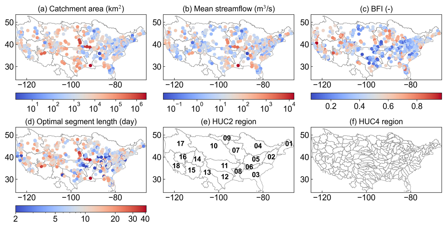
Figure 1 Spatial distribution of the 855 selected catchments with their drainage area (a), mean streamflow (b), BFI (c), and optimal segment length parameter N (d) superimposed on HUC2 regions. The HUC2 and HUC4 region maps are provided for referencing (e, f).

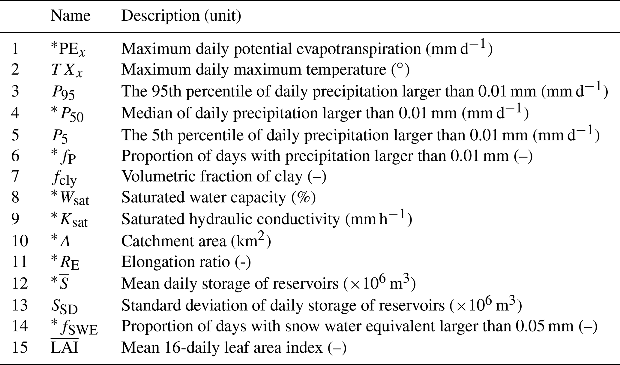
Lin et al. (2026) identified 13 catchment characteristics representing the geomorphology, climate, soil hydraulic properties, and water usage, that significantly influence the SMM parameter N (Table 1, rows 1–13). In addition to these predictors, we added two more related to snow processes and vegetation dynamics (Table 1, rows 14–15), as previous studies have shown that these factors can substantially affect baseflow generation (Price, 2011; Stoelzle et al., 2020; Xie et al., 2022). The data of these 15 variables are all obtained from Lin et al. (2025). To reduce the dimensionality of the predictor space, we examined the mutual information (MI) between candidate predictors. Variable pairs exhibiting MI values greater than 0.5 were considered to contain substantial shared information (Fig. S1 in the Supplement). In such cases, only one representative variable was retained to prevent redundant contributions in training the symbolic regression models. After this screening step, the number of predictors was reduced to nine (highlighted in blue in Table 1), which were then used as inputs for the SR analysis.

Table 1 Catchment characteristics used as inputs to the SR method for predicting parameter N. Catchment characteristics marked with an asterisk are selected for the development of SR based on the mutual information approach.

3 Methods

3.1 Smooth Minima Baseflow Separation

SMM is a widely used baseflow separation method (Aksoy et al., 2008; Piggott et al., 2005; Xie et al., 2020; Tan et al., 2020). It assumes that total streamflow is partitioned into baseflow and event-flow components and baseflow constitutes 100 % of streamflow during low-flow periods (Gustard et al., 1992). The SMM procedure involves partitioning daily streamflow into non-overlapping N-day intervals and identifying the minimum value within each segment. These minimum points (Q₁, Q₂, Q_i, …) are then screened using a filtering coefficient (M): a point is discarded if M⋅Q_i exceeds the value of either adjacent minimum. Finally, the baseflow series is constructed by linearly interpolating the remaining minima. The method involves two key parameters: the segment length parameter (N) and the filtering coefficient parameter (M). The segment length parameter N is a proxy of the flow event duration (Stoelzle et al., 2020). Generally, a smaller N results in a higher proportion of baseflow in streamflow, implying shorter surface flow duration. In the literature, N often defaults to 5 d or is predicted using a power-law relationship with catchment area, namely $N=\mathrm{1.6}\times A^{\mathrm{0.2}}$, where A is the catchment area in km² and N is expressed in days (Zhang et al., 2017; Aksoy et al., 2008). These two formulations of N are included in the comparison and are denoted as F_D and F_PL, respectively. To further examine the explanatory capacity of the areal-based power-law relationship, we considered a calibrated form of $N=a\cdot A^b$ (denoted as $F_{\mathrm{PL}}^{\prime }$), where the coefficients a and b are estimated from the data by minimizing the squared error between the reference and predicted Ns.

The filtering coefficient parameter M is used to determine if a streamflow minimum qualifies as a strict baseflow point. Higher values of M (typically not exceeding 1) correspond to more stringent criteria for identifying pure baseflow conditions. Unlike N, the parameter M is less sensitive to the baseflow separation results and is commonly assigned a constant value of 0.9 (Stoelzle et al., 2020; Aksoy et al., 2008).

3.2 Symbolic regression modelling for the segment length parameter

Symbolic regression (SR) is employed to derive expressions for the parameter N. SR represents an expression using a tree structure, where each node corresponds to a mathematical operator, and each leaf represents an input variable or constant. Structure of the tree evolves to identify expressions that best fit the inputted data through genetic programming (Koza, 1994). Five sample SR trees were demonstrated within the dotted box in Fig. 2a. In this study, the SR method is implemented using the PySR library in Python (Cranmer, 2023), which enforces syntactically valid mathematical structures through predefined operator sets and expression tree representations. The nine representative catchment attributes in original units (Table 1) were used as predictors without normalization to maintain interpretability for the SR expressions. The function space consists of the catchment attributes, free constants, and a set of mathematical operators: addition (+), subtraction (−), multiplication (×), division ($/$), power-law (power), and logarithm (log).

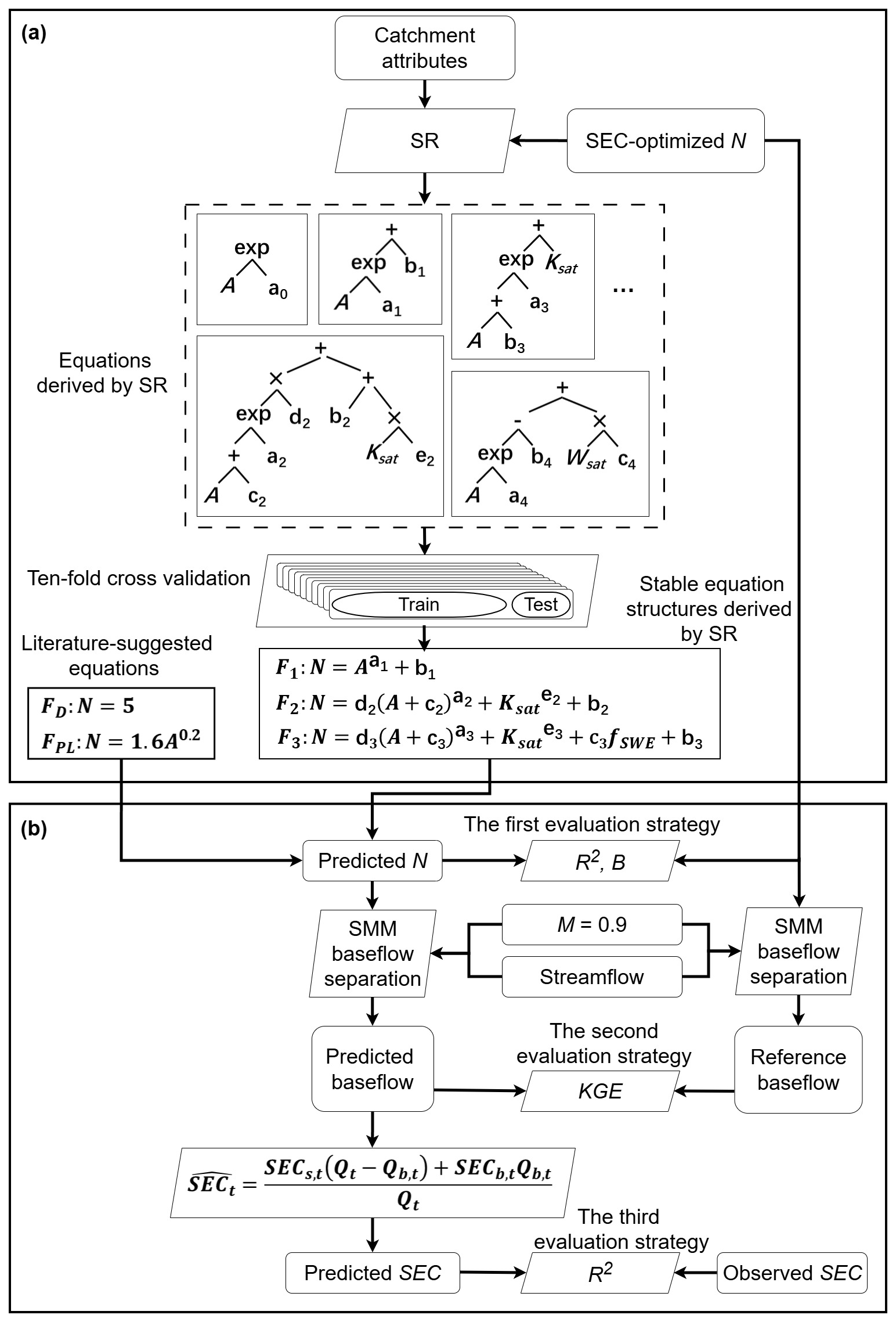
Figure 2 Flowchart of the SR-based prediction framework for the parameter N of SMM (a) and the three performance evaluation strategies (b).

To control the search space and ensure physically interpretable expressions, several structural constraints were imposed in SR model training. Multiplication, division, power-law, and logarithmic operators were not allowed to be nested within operators of the same type. The internal complexity of expressions inside power-law and logarithmic operators was restricted to a maximum value of 3. The maximum allowable total complexity was set to 20. Expression complexity is defined as the sum of the complexity index assigned to each component in the equation. Take $N=\mathrm{1.6}\times A^{\mathrm{0.2}}$ as an example, if multiplication and power-law operators are each assigned a complexity of 2 and constants and input variables are assigned a complexity of 1, the total complexity of the expression is calculated as $\mathrm{2}+\mathrm{2}+\mathrm{1}+\mathrm{1}+\mathrm{1}=\mathrm{7}$. In this study, all operators were assigned a uniform complexity index of 1 to avoid bias toward specific functional forms. Recursive formulations (i.e., expressions where the output variable appears as an input to itself) were not permitted to ensure model interpretability and avoid trivial or ill-posed solutions.

The SR search process was configured with the following hyperparameters: a population size of 33, populations of 15, the crossover rate of 0.066, and evolved over 40 generations. The goodness of fit between the reference and the predicted Ns is evaluated using the mean squared error (MSE):

$$\begin{array}{}\text{(1)}& \mathrm{MSE}={\displaystyle \frac{\mathrm{1}}{C}}\sum _{i=\mathrm{1}}^C{\left(N_i-{\widehat{N}}_i\right)}^{\mathrm{2}},\end{array}$$

where C is the total number of catchments, and N_i and ${\widehat{N}}_i$ represent the reference and predicted values of N for catchment i, respectively. To evaluate the robustness of the SR models, a ten-fold cross-validation strategy is employed (Fig. 2a). The 855 catchments are randomly partitioned into ten subsets of approximately equal size. In each iteration, the model is trained on nine subsets and tested on the remaining one to estimate the generalization error. This process is repeated ten times so that each subset serves once as the testing set. In each iteration, 7 to 10 expressions with varying levels of complexity are generated, resulting in a total of 91 expressions. Among these expressions, we identified recurrent equation forms across all ten iterations.

3.3 Evaluation strategies

Three strategies are employed to evaluate the performance of different Ns calculated by the SR formulas (Fig. 2b). The first strategy compares the predicted and reference Ns using the mean bias (B) and coefficient of determination (R²):

$$\begin{array}{}\text{(2)}& {\displaystyle }B={\displaystyle \frac{\mathrm{1}}{C}}{\sum }_{i=\mathrm{1}}^C\left(N_i-{\widehat{N}}_i\right),\text{(3)}& {\displaystyle }{R}^{\mathrm{2}}={\displaystyle \frac{{\sum }_{i=\mathrm{1}}^C{\left(N_i-{\stackrel{\mathrm{‾}}{N}}_r\right)}^{\mathrm{2}}-{\sum }_{i=\mathrm{1}}^C{\left(N_i-{\widehat{N}}_i\right)}^{\mathrm{2}}}{{\sum }_{i=\mathrm{1}}^C{\left(N_i-{\stackrel{\mathrm{‾}}{N}}_r\right)}^{\mathrm{2}}}},\end{array}$$

where ${\stackrel{\mathrm{‾}}{N}}_r=\frac{\mathrm{1}}{C}\sum _{i=\mathrm{1}}^C{N}_i$ is the mean of the reference N over all catchments. Positive (negative) Bs indicate overestimation (underestimation), with lower magnitudes suggesting better performance. R² measures the proportion of variance explained by the prediction; it ranges from 0 to 1, with higher values indicating better agreement.

The second strategy evaluates the SR-derived N values in the context of baseflow separation using the SMM method. Specifically, the SMM baseflow time series are calculated using different N values with the other parameter M fixed at 0.9 to eliminate its influence. Baseflow time series calculated with the reference N for each catchment (N_i) is used as the reference. The similarity between the calculated and reference baseflow is assessed using the Kling-Gupta Efficiency (KGE) metric (Gupta et al., 2009):

$$\begin{array}{}\text{(4)}& \mathrm{KGE}=\mathrm{1}-\sqrt{{\left(\mathit{\rho }-\mathrm{1}\right)}^{\mathrm{2}}+{\left({\displaystyle \frac{{\mathit{\sigma }}_p}{{\mathit{\sigma }}_r}}-\mathrm{1}\right)}^{\mathrm{2}}+{\left({\displaystyle \frac{{\mathit{\mu }}_p}{{\mathit{\mu }}_r}}-\mathrm{1}\right)}^{\mathrm{2}}},\end{array}$$

where ρ is the correlation coefficient between the predicted and reference baseflow, and μ and σ denote the mean and standard deviation of baseflow. KGE ranges from negative infinity to 1, with higher values indicating better agreement.

The third strategy compares SEC calculated using the SMM baseflow with the observed SEC. Specifically, baseflow time series generated by SMM using Ns derived by the constant, the power-law, and the three SR formulas are used to estimate SEC based on the chemical and water balance relationship:

$$\begin{array}{}\text{(5)}& \widehat{{\mathrm{SEC}}_t}={\displaystyle \frac{{\mathrm{SEC}}_{\mathrm{s},t}\left(Q_t-B_t\right)+{\mathrm{SEC}}_{\mathrm{b},t}{B}_t}{Q_t}},\end{array}$$

where Q_t and B_t are the observed streamflow and the predicted baseflow at time t, respectively; SEC_s,t and SEC_b,t are the surface flow and baseflow SEC concentrations, respectively. The values of SEC_s,t and SEC_b,t are derived using the extreme value interpolation method, which connects the monthly maxima and minima of the observed SEC with spline interpolation to represent the stable variation of SEC in each of the flow components (Mei et al., 2024b). The derivation of Eq. (5) is documented in Supplement Sect. S1 in the Supplement. The agreement between observed and predicted streamflow SEC is assessed using the R² metric (Eq. 1).

To assess whether the differences in SR-based SEC prediction performance are statistical significant, we apply the Diebold–Mariano (DM) test (Diebold and Mariano, 1995). Details on procedure and test statistics are provided in Section S2 in the Supplement. For each catchment, pairwise DM tests are performed among the three SR formulas to determine whether their SEC R² differences are statistical significance at the 0.01 significance level. If the largest R² is significantly different from the second-largest R², the SR formula associated with the largest R² is the single best formula of the catchment. If the difference between the largest and the second-largest R²s is insignificant but that between the second and the third ones is significant, the first two SR formulas are tied. Otherwise, the three SR are tied. Based on these catchment-scale rankings, the best-performing formula for the HUC2 and HUC4 regions is determined as the one most frequently ranked as the best among all catchments within the regions.

4 Results

4.1 SR expressions for N predictions

Three SR formulas with identical functional structures and increasing complexity levels of 5, 13, and 17 were consistently identified across the ten cross-validation iterations. As summarized in Table 2, the simplest formulation is $F_{\mathrm{1}}:N=A^{a_{\mathrm{1}}}+b_{\mathrm{1}}$, followed by the intermediate formulation $F_{\mathrm{2}}:N=d_{\mathrm{2}}(A+c_{\mathrm{2}}{)}^{a_{\mathrm{2}}}+(K_{\mathrm{sat}}{)}^{e_{\mathrm{2}}}+b_{\mathrm{2}}$, and the most complex formulation $F_{\mathrm{3}}:N=d_{\mathrm{3}}(A+c_{\mathrm{3}}{)}^{a_{\mathrm{3}}}+(K_{\mathrm{sat}}{)}^{e_{\mathrm{3}}}+f_{\mathrm{3}}\cdot f_{\mathrm{SWE}}+b_{\mathrm{3}}$. The optimized coefficients of these replicated formulas vary only within narrow ranges (Table 2), indicating a high degree of consistency in parameterization across folds. From F₁ to F₃, the SR results progressively incorporate A, K_sat, and f_SWE, suggesting that catchment size, subsurface permeability, and snow processes jointly govern the variability of N. The repeated identification of these three formulations across all iterations further demonstrates their structural robustness for predicting N. Accordingly, subsequent analyses focus on these three formulas.

Table 2 The calibrated $F_{\mathrm{PL}}^{\prime }$ and the three stable SR expressions across all ten iterations of the cross-validation. The numbers within the brackets of the first row are the complexity of the expressions.

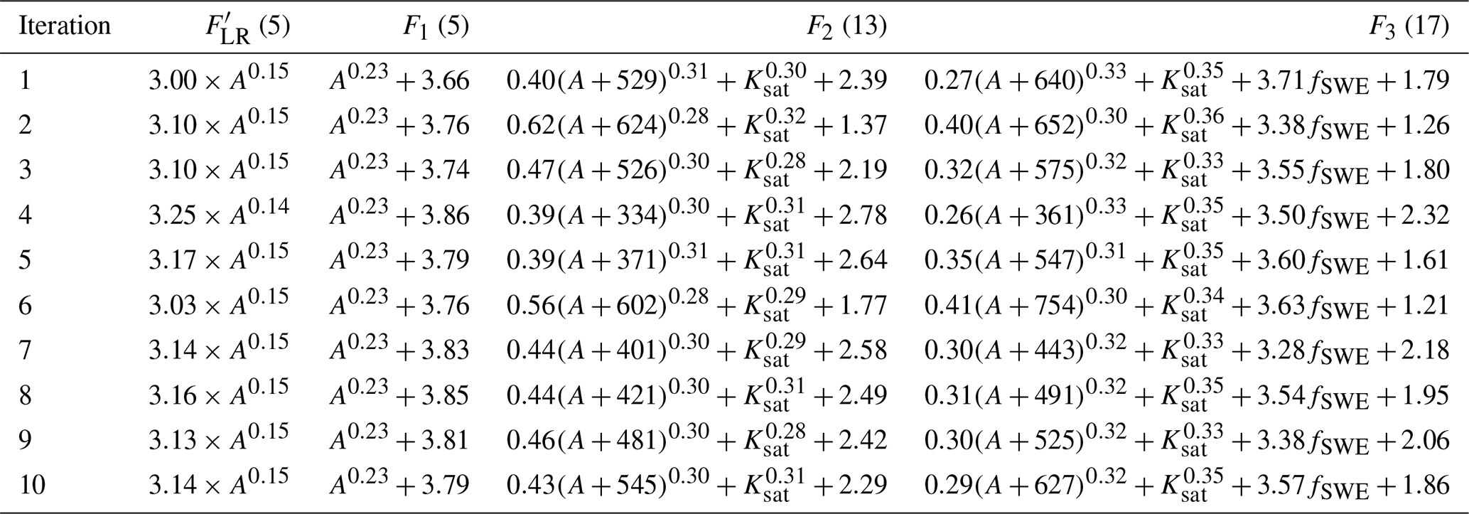
Figure 3 further illustrates the behavior of these formulas. For F₁, the nearly identical exponents (∼ 0.23) and intercepts (3.66–3.86 d) result in almost overlapping curves (Fig. 3a), indicating a stable power-law relationship between N and A, with a diminishing rate of increase. For F₂, the similarly constrained exponents (0.28–0.32) and intercepts (1.37–2.78 d) produce tightly clustered response curves (Fig. 3b–c), showing that both A and K_sat contribute positively to N. F₃ extends F₂ by introducing f_SWE as a linear term. The replicated formulas still exhibit closely grouped slopes (3.28–3.71 d) and intercepts (1.21–2.32 d), which explains the clustering of curves in Fig. 3d–f. The marginal relationships of N with A and K_sat in F₃ remain consistent with those in F₂, whereas increasing f_SWE leads to an approximately linear increase in N, at a rate of about 0.3–0.4 d per 0.1 increment in snow fraction. Overall, SR identifies A as the most influential factor in predicting N, as evidenced by its presence in all SR-derived formulas. The narrower ranges of predicted Ns in Fig. 3b and d also suggest that A exerts greater influence than K_sat and f_SWE.

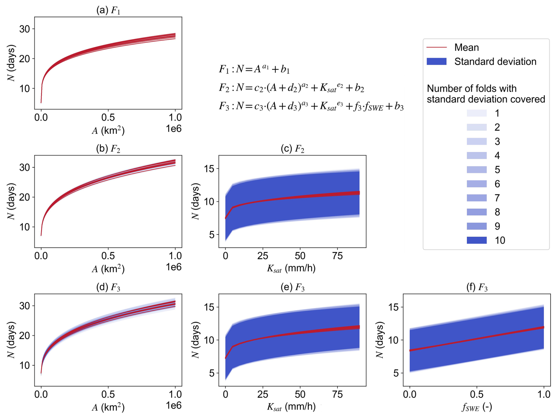
Figure 3 Marginal relationship of N on different predictors (A, K_sat, and f_SWE) that consist of the SR expressions (F₁, F₂, and F₃). Each line represents one of the ten instances of F₁, F₂, and F₃. Panels a, b, and d are for A; panels (c) and (e) are for K_sat; panel f is for f_SWE.

4.2 Evaluation of N predictions

Figure 4 presents the performance of N predicted using the two literature-suggested formulas (F_D and F_PL) and the three SR formulas (F₁, F₂, and F₃) for the ten training and testing sets. It should be noted that the literature-suggested formulas do not require training; instead, they are directly applied to the training and testing sets separately. Overall, the performance of formula F_D is poor, with negative R² values less than −0.6. F_PL shows higher performance but still yields modest R² medians of 0.23 and 0.22 for the training and testing sets, respectively. The calibration with respect to SEC data improves the performance for $F_{\mathrm{PL}}^{\prime }$ to median R² values of 0.43 and 0.42 for the training and testing sets, respectively, and R² of 0.42 for the combined testing set. For predictions from the three SR-derived formulas, we observed higher performance than the conventional formulas. The R² medians for F₁, F₂, and F₃ are 0.49, 0.53, and 0.56 for the training sets, and 0.45, 0.49, and 0.55 for the testing sets, respectively. The overall R² values for the ten testing sets together for F₁, F₂, and F₃ are 0.48, 0.52, and 0.55, respectively. In terms of the bias, the SR-derived formulas significantly reduce the underestimation of N by the conventional formulas (Fig. 4b). The medians B for F₁, F₂, and F₃ are $\mathrm{0.00}/\mathrm{0.06}$, $\mathrm{0.00}/\mathrm{0.08}$, and $\mathrm{0.00}/-\mathrm{0.03}$ d for the training/testing sets, respectively, comparing to F_D and F_PL at $-\mathrm{4.44}/-\mathrm{4.38}$ and $-\mathrm{2.34}/-\mathrm{2.28}$ d. These values for the combined testing set are −4.44, −2.33, 0.00, 0.00 and 0.00 d for F_D, F_PL, F₁, F₂, and F₃, respectively. It is noteworthy that the testing sets exhibit wider ranges of R² and B values compared to the training sets. This variability is primarily attributed to the differences in catchment attributes of the testing samples rather than the discrepancies among the 10 replicated formulas. This is supported by the nearly identical coefficients (i.e., a, b, and c) in the SR formulas (Table 2).

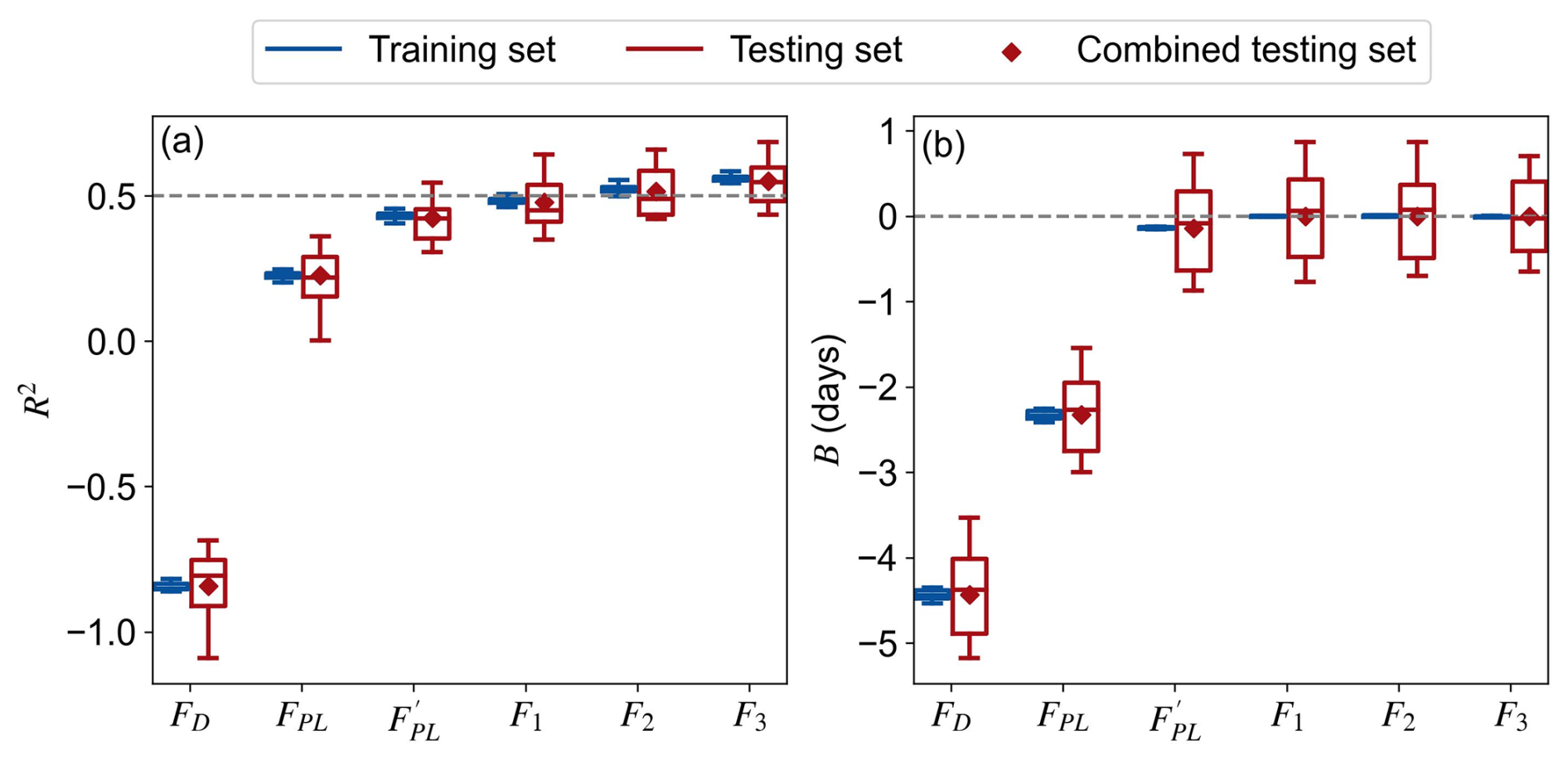
Figure 4 Performance of N predictions using the constant (F_D), power-law (F_PL), calibrated power-law ($F_{\mathrm{PL}}^{\prime }$), and the three SR formulas (F₁, F₂, and F₃) for the ten training and testing sets of the 10-fold cross-validation: coefficient of determination R² (a) and mean bias B (b).

4.3 Application of N predictions in baseflow separation

Figure 5a reveals the baseflow separation performance of different N predictions measured by KGE for the testing sets. The baseflow separation performance roughly follows the ranking of $F_{\mathrm{D}}<F_{\mathrm{PL}}<F_{\mathrm{PL}}^{\prime }<F_{\mathrm{1}}<F_{\mathrm{2}}<F_{\mathrm{3}}$, in line with the N predictions (Fig. 4). The median KGEs for F_D, F_PL, $F_{\mathrm{PL}}^{\prime }$, F₁, F₂, and F₃ are 0.63, 0.73, 0.83, 0.84, 0.84, and 0.85, respectively. For F_D and F_PL, 12 % and 5 % of catchments exhibit KGE <0, while 64 % and 78 % report KGE >0.5, respectively. In contrast, the percentage of catchments with KGE <0 drops to 1 % for $F_{\mathrm{PL}}^{\prime }$, F₁, F₂, and F₃, and those with KGE >0.5 rise to more than 85 %. These observations indicate the benefits of performing regional calibration for the N prediction.

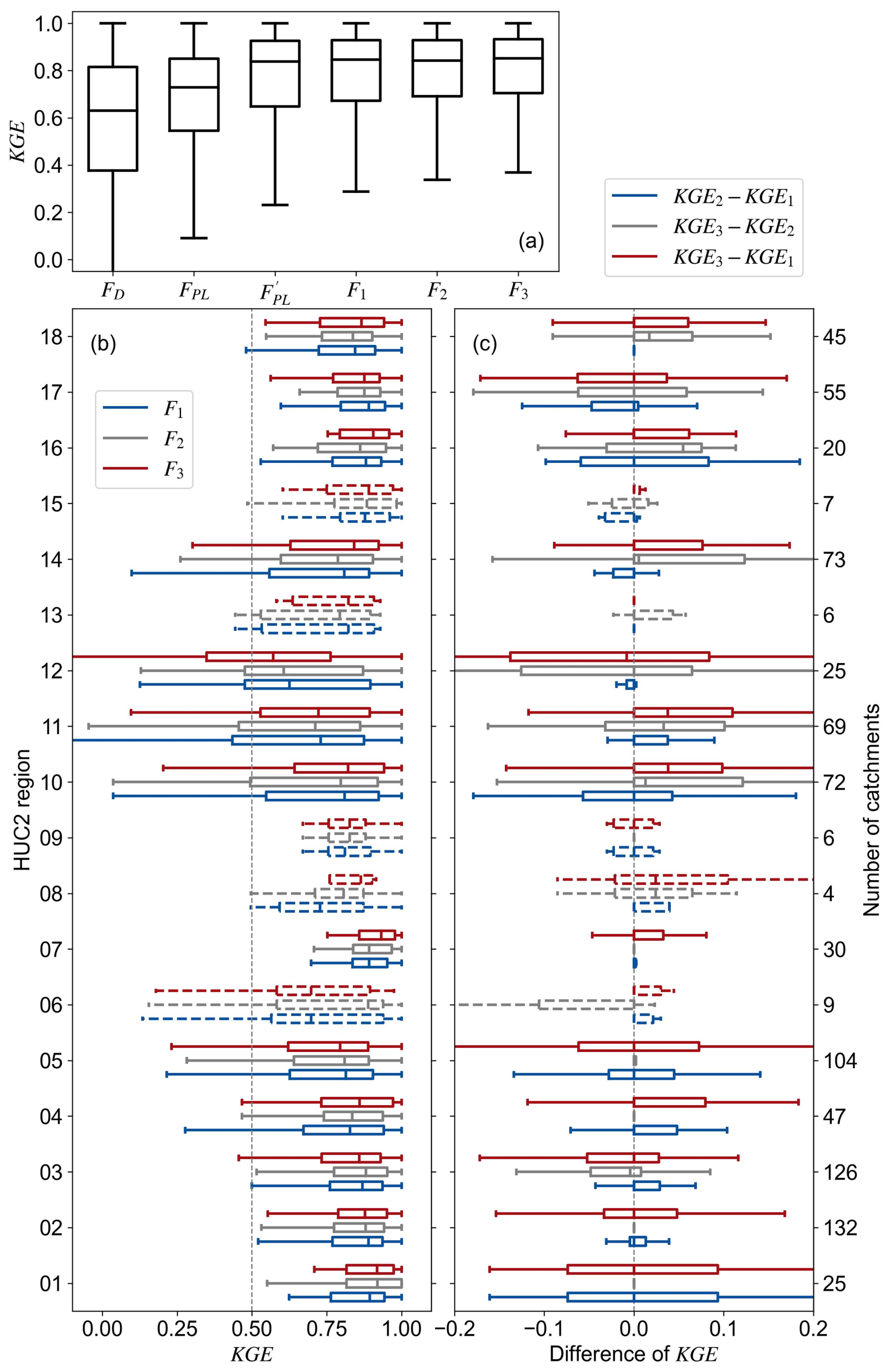
Figure 5 Baseflow separation performance based on different N predictions for all catchments (a) and for catchments of the 18 HUC2 regions (b), and relative performance between each pair of the three SR cases for the HUC2 regions (c). Regions with fewer than 10 catchments are plotted by dashed lines in panels (b) and (c).

Figure 5b shows the performance of the three SR formulas across the 18 HUC2 regions. Overall, all formulas perform well for the HUC2 regions, with median KGEs ranging from 0.57 to 0.93. The best performing regions for F₁, F₂, and F₃ are HUC 02, 01, and 07, respectively, exhibiting median KGE values above 0.89 and over 95 % of catchments achieving KGE values greater than 0.5. In contrast, the lowest performance for all three formulas occurs in HUC 12, where median KGE values fall below 0.65 and more than 25 % of catchments show KGE values below 0.5. This may be related to the relative arid climate and flashy hydrological response of HUC 12 (Kratzert et al., 2019; Feng et al., 2020), which is difficult for SMM to capture. Note that SMM is more skillful for smooth baseflow dynamics (Stewart, 2015). All three formulas exhibit larger performance variability in HUC 10–12 and 14 compared to other regions. This can be attributed to the fact that these regions are mountainous and plain areas, characterized by relatively high heterogeneity in catchment characteristics.

Figure 5c compares the relative performance of F₁, F₂, and F₃ across regions. F₂ outperforms F₁ for HUC 04-09 located in the northern and northeastern CONUS, while it performs worse than F₁ in HUC 12–15 on the south. F₃ generally outperforms F₂ in the mountainous region spanning HUC 10–11 and 13–18, and shows comparable performance to F₂ in HUC 01, 02, 04, 05, and 07 with mild topography. In HUC 02, 04, 07, 08, 10, 11, 13, 14, 16, and 18, the most complex F₃ outperforms the other SR formulas. However, F₃ performs worse than F₁ and F₂ in HUC 12. This may be because the SR formulas were calibrated using all catchments to optimize performance at the CONUS scale; thus, their region-specific performance inevitably reflects trade-offs. In relatively warm regions such as HUC 12, where snow influence is weak, the SWE term included in F₃ may add unnecessary complexity rather than useful information, resulting in slightly poorer performance than F₁ and F₂.

Figure 6 presents the average KGE of baseflow separation as functions of the three influential catchment attributes. Overall, the SR formulas consistently outperform the literature-suggested formulas for most of the predictor value ranges, with relatively minor performance differences among F₁, F₂, and F₃, highlighting their robustness across diverse catchment conditions. According to Fig. 6a, when A exceeds 300 km², corresponding to N=5 d by F_PL, the performance of F_D deteriorates markedly. This suggests that using N=5 d cannot adequately represent its variation for larger As. Conversely, for A < 300 km², the performance of F_PL declines, indicating that the power function coefficients are not suitable for smaller catchments over CONUS. The calibrated power-function ($F_{\mathrm{PL}}^{\prime }$) reveals improved performance to a similar level with the SR formulas except for the A < 100 km² bin, indicating the necessity regional calibration. Across the full range of A, the SR formulas consistently achieve higher KGE values, emphasizing the benefits of regional calibration. For small catchment (A < 100 km²), accounting for f_SWE and K_sat leads to performance gains. In contrast, for larger basins (A > 100 km²), the additional contribution of these factors becomes negligible.

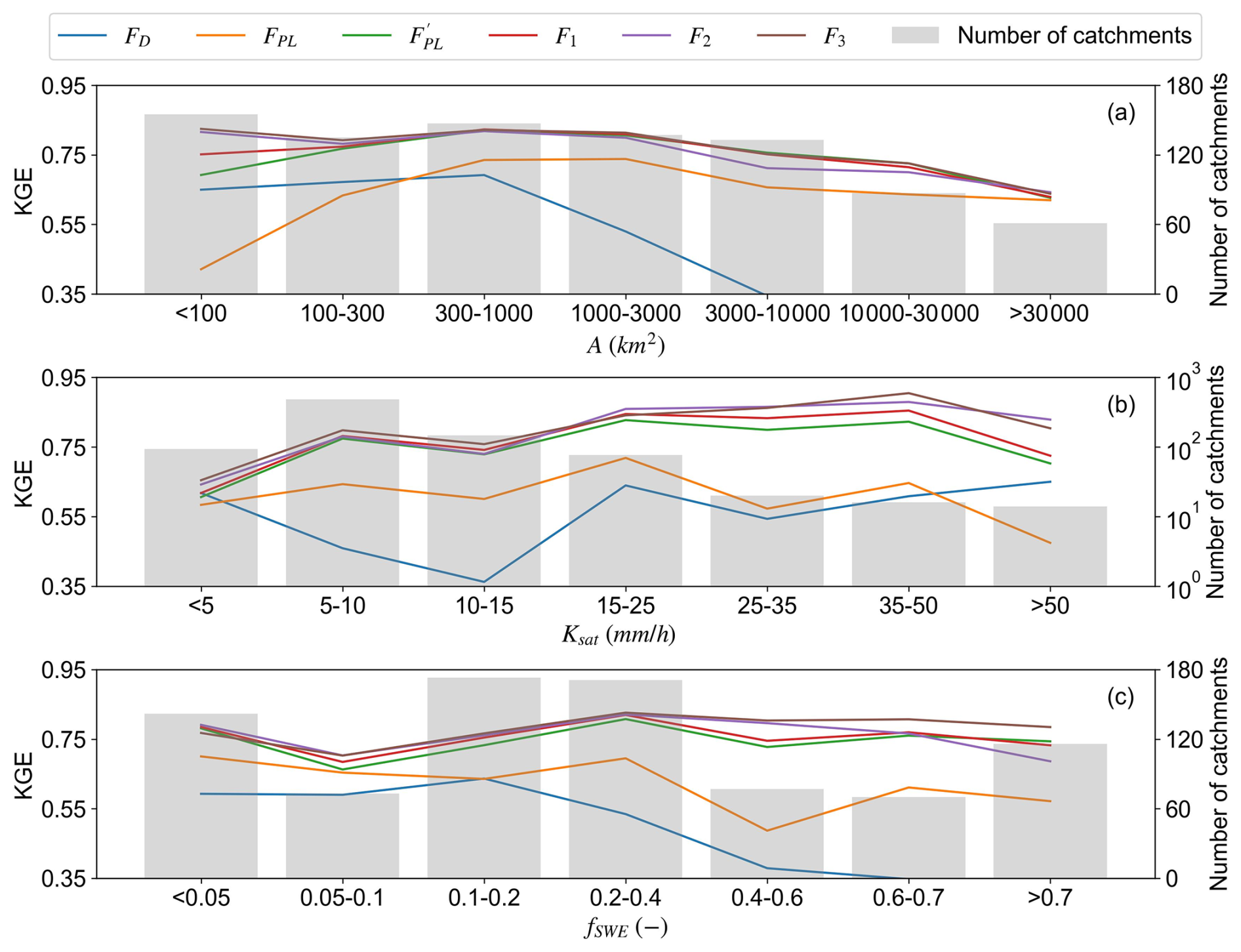
Figure 6 Performance of baseflow separation for different ranges of catchment area (a), catchment-averaged saturated hydraulic conductivity (b), and snow day fraction (c). The right y-axis for panel (b) is in logarithmic scale.

Figure 6b examines the influence of K_sat. When K_sat < 5 mm h⁻¹, all predictions show similar level of baseflow prediction performance, suggesting that K_sat is not a major factor for catchments with low soil hydraulic conductivity. In the intermediate ranges (5–25 mm h⁻¹), the two regionally fitted power-law formulas (F₁ and $F_{\mathrm{PL}}^{\prime }$) outperform the conventional power-law formula (F_PL). Although F₁ and $F_{\mathrm{PL}}^{\prime }$ do not explicitly include K_sat, their performance remains comparable to F₂ and F₃, which incorporate K_sat. This indicates that regional fitting may compensate the effects of K_sat for small and medium values. When K_sat > 25 mm h⁻¹, incorporating K_sat substantially improves the predictions, highlighting the increasing importance of subsurface processes in highly permeable catchments. Figure 6c reveals the influence of f_SWE. F₃ outperforms all formulas when f_SWE > 0.4, indicating the importance of f_SWE for catchments with stronger snow persistency. In contrast, for f_SWE < 0.4, $F_{\mathrm{PL}}^{\prime }$, F₁, and F₂ perform similarly to F₃, demonstrating that regionally calibrated coefficients can partially offset the lack of explicit consideration of snow-related variables.

4.4 Estimation of SEC variation based on predicted N

The SEC estimation performance by different N predictions for the testing set is evaluated using R². The median R² values range from 0.70 to 0.74 for the F_D, F_PL, $F_{\mathrm{PL}}^{\prime }$, F₁, F₂, and F₃ formulas, with similar interquartile ranges between 0.29 and 0.33, indicating relatively small overall differences among formulas. Despite these modest differences, both the medians and interquartile ranges of R² follow a clear order of $F_{\mathrm{D}}<F_{\mathrm{PL}}<F_{\mathrm{PL}}^{\prime }<F_{\mathrm{1}}<F_{\mathrm{2}}<F_{\mathrm{3}}$. This ranking is consistent with both the N predictions (Fig. 4) and the baseflow separation results (Fig. 5). The mean R² differences between most formulas are statistically significant, except for the comparison between F₁ and F₂ (p≥0.01).

Figure 7 illustrates the spatial distribution of the best-performing formulas across the HUC4 regions. F₃ demonstrates superior performance across most of the mountainous regions, including the Rocky Mountain foothills, Cascade Range, Sierra Nevada, and some regions within the Great Plains. The improvement for the mountainous regions is likely due to the explicit incorporation of f_SWE in the SR formula, capturing the influence of snow processes; for the relatively flat Great Plains regions, the improvement is primarily driven by the consideration of K_sat, which better represents subsurface processes such as infiltration capacity, percolation, and lateral subsurface flow that regulate groundwater recharge and baseflow contributions. In contrast, F₁ performs best in the eastern and southeastern CONUS, including the Appalachian Mountains, coastal plain, and Florida peninsular, where the effects of K_sat and f_SWE are minimal. These regions are generally characterized by low BFI values (Fig. 1c), indicating surface runoff-dominated streamflow with limited relevance of delayed-flow processes (Wu et al., 2021; Mcmillan, 2020). F₁ achieves the highest performance in fewer HUC4 regions, indicating that the effects of K_sat may be compensated by the regional calibration of F₁. Interestingly, several regions located in the Great Plains exhibit mixed optimal performance for multiple formulas, suggesting a more complex interplay of hydrological drivers in these areas.

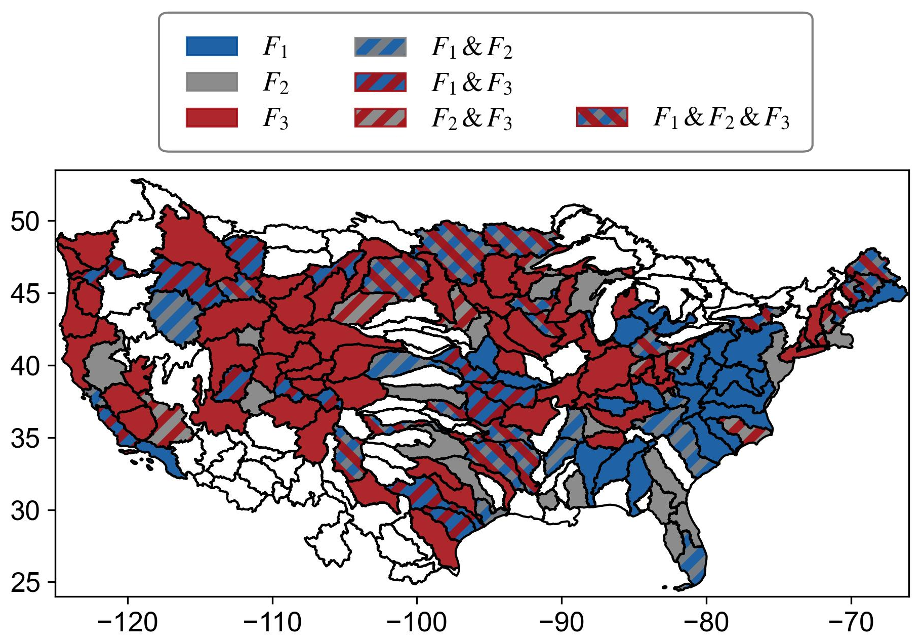
Figure 7 Spatial distribution of the best-performing formulas for SEC estimations across different HUC4 regions. At the HUC4 scale, the best-performing formula is the one(s) appears most frequently as the best among all catchments within the region.

5 Discussions

5.1 Regionalization of baseflow separation parameter by SR

In this study, we used SR to derive mathematical expressions for the predictions of N using 9 catchment attributes. Across ten cross-validation iterations, the identified expressions exhibited consistent structures, predictors, and nearly identical regression coefficients, indicating that SR can yield stable functional relationships between catchment attributes and N. Compared to the RF-based predictions reported by Lin et al. (2026), the SR-based approach showed lower predictive skill (R²= 0.54 vs. 0.80), reflecting the trade-off between predictive accuracy and interpretability. While RF achieves superior predictive performance, it functions as a “black-box” ensemble, offering no explicit functional form to clarify whether environmental controls operate additively, multiplicatively, or through nonlinear transformations. In contrast, SR provides structural transparency by yielding a closed-form equation, facilitating direct analytical insights (Karpatne et al., 2024; Häfner et al., 2023). This explicit representation enables rigorous sensitivity analysis via differentiation; for instance, the marginal effects derived from equation F₃ quantify how geomorphic and climatic factors jointly govern N. By trading a degree of predictive skill for parsimony, SR transforms the problem from simple estimation into a hypothesis-generating exercise, providing compact transfer functions that are easily integrated into regionalization frameworks (Feigl et al., 2022; Samaniego et al., 2010). Therefore, RF and SR should be viewed as complementary rather than competing approaches: RF provides a benchmark for predictive performance, while SR offers structural transparency that facilitates theoretical interpretation and model integration.

One important aspect to consider when training SR models is the diversity of mathematical operators. A wide variety of operators for model training enables the discovery of complex relationships among variables, but it also enlarges the search space, increasing training time and risk of overfitting (Li et al., 2025; Elsken et al., 2019). To address these challenges, we adopted two strategies. First, we incorporated domain knowledge to guide the choice of operators. Specifically, the well-established power-law relationship between streamflow response time and catchment area motivated the inclusion of the power-law operator in the SR operator set. The fact that all SR-derived formulas captured this power-law relationship indicates the effectiveness of using this domain knowledge. Second, cross-validation was applied to assess model generalizability and reduce overfitting, ensuring representativeness of the SR expressions across the catchments. Although SR can generate more complex formulas than F₃ with better training fit, these structures are inconsistent across folds. This suggests that they may overfit specific subsets of the data and lack generalizability, and are therefore excluded from our analysis.

5.2 Influential catchment attributes for N predictions

The segment length parameter N is a proxy of the average duration of surface flow, and larger values indicate surface flow of event sustain for longer time on average (Stoelzle et al., 2020). Our findings indicate that N is a power function of catchment area with exponent of 0.22–0.23 (F₁, Table 2), indicating that larger catchments are characterized by longer average surface flow duration (Garzon et al., 2023; Mei and Anagnostou, 2015), and the increasing rate in duration slows down for larger As. This could be attributed to the longer averaged water paths for larger catchments (i.e., the Hack's Law), increasing the average traveling time for surface flow of event (Tarasova et al., 2024). Saturated hydraulic conductivity is another key factor in the predictions of N: N increases according to the power-law functions with exponents of 0.28–0.36 with respect to K_sat (F₂ and F₃ in Table 2). This indicates that higher K_satvalues tend to increase the average duration of surface flow with decreasing rate. A possible explanation is that catchments with higher K_sat tend to promote infiltration, making more rainfall excess to route through the slow subsurface flow paths than the rapid overland ones (Nagy et al., 2024). F₃ reveals that prolonged snow cover (higher fraction of days covered by snow) is linearly associated with longer surface flow duration. This is due to the snowpack acting as a seasonal storage that modulates streamflow timing (Stoelzle et al., 2020). The gradual melting of snowpack slowly released meltwater to the stream networks, increasing the time needed to leave the catchment (Noor et al., 2023; Barnhart et al., 2016; Godsey et al., 2014). Overall, the additive structure among A, K_sat, and f_SWE reflect the separate contributions of different catchment-scale delay processes to the event flow through different pathways and at different time scales. Their additive combination therefore provides a parsimonious empirical approximation of the integrated flow-duration response.

5.3 Trade-off between formula complexity and prediction accuracy

Our experiments reveal that formulas for baseflow separation with higher structural complexity generally achieve better predictive performance. This is because more complex formulas can incorporate additional predictors for more detailed descriptions of the underlying hydrological processes. However, the predictive gain from increased complexity is not uniform across all hydro-climatic conditions. For example, when K_sat and f_SWE take relatively small values (K_sat < 25 mm h⁻¹ and f_SWE < 0.4), the performance differences among F₁, F₂, and F₃ are minimal (Fig. 6). This is likely because small variations in K_sat and f_SWE have limited impact to the prediction, allowing the regional calibration to partially compensate for the absence of these variables in the formulas. However, such compensation is limited for large K_sat and f_SWE (K_sat > 25 mm h⁻¹ and f_SWE > 0.4), where their influence becomes more pronounced (Jenicek and Ledvinka, 2020; Beven and Germann, 2013). Moreover, the effects of K_sat and f_SWE are more evident when A is smaller than 100 km² (Fig. 6a). As catchment area increases (A > 100 km²), their influence is outweighed by A, highlighting the dominant role of drainage area in shaping the streamflow response time (McGlynn et al., 2004; Sólyom and Tucker, 2007).

6 Conclusions and future work

In this study, we applied symbolic regression to derive formulas for the prediction of segment length parameter N (a proxy of the average duration of surface flow) of the smooth minima baseflow separation method across 855 CONUS catchments. Three stable formulas with increasing complexity were identified: $N=A^{a_{\mathrm{1}}}+b_{\mathrm{1}}$, $N=d_{\mathrm{2}}(A+c_{\mathrm{2}}{)}^{a_{\mathrm{2}}}+(K_{\mathrm{sat}}{)}^{e_{\mathrm{2}}}+b_{\mathrm{2}}$, and $N=d_{\mathrm{3}}(A+c_{\mathrm{3}}{)}^{a_{\mathrm{3}}}+(K_{\mathrm{sat}}{)}^{e_{\mathrm{3}}}+f_{\mathrm{3}}\cdot f_{\mathrm{SWE}}+b_{\mathrm{3}}$, where catchment area (A), saturated hydraulic conductivity (K_sat), and snow day fraction (f_SWE) are identified as important predictors. These SR formulas showed substantial improvements in predictive accuracy of N comparing to the constant (N=5) and power-law formula (N=1.6A^0.2). The SR-derived Ns also reveal better performance in baseflow separation and in estimation of electrical conductance dynamics. Among the three SR formulas, F₃ performs better in regions influenced by snow, such as the mountainous mid-west and the northern CONUS; F₁ shows better performance in the eastern and southeastern CONUS, where both the climate and terrain are mild and infiltration rate is low. Overall, formulas that consider K_sat and f_SWE tend to yield higher predictive accuracy, but simpler formulas without K_sat or f_SWE can still achieve comparable performance when the values of these key predictors are relatively small. This study presents a new paradigm for regionalization of optimal baseflow parameters using symbolic regression and demonstrates its potential to improve model interpretability and transferability across diverse catchments.

This study used all gages across CONUS to train SR. However, the influence of catchment attributes on N varies across regions. Future work could explore the benefits of developing region-specific SR formulas for different catchment clusters to improve the prediction performance. Furthermore, this study investigated SR-based modeling of only one parameter of a baseflow separation method. Future research could explore applying SR to other baseflow separation methods to identify the governing equations relating catchment attributes to the parameters of these methods. This may help to understand how catchment attributes influence the partitioning of streamflow.