A novel classifier-guided ensemble framework for global terrestrial evapotranspiration estimates

Evapotranspiration (ET) is a key hydrological and meteorological variable, serving as the critical nexus between water and energy exchanges. However, accurate estimation of global ET remains a challenging task, as process-based ET algorithms are often inadequate to capture the nonlinear relationship among environmental factors, and the application of data-driven ET algorithms is hindered by sparse and uncertain ET observations. In this study, we developed a novel ensemble framework that integrates three existing ET models (process-based algorithm, machine learning-based ET model, and hybrid model), aiming to provide high-precision terrestrial ET estimates. The framework is guided by an additional classifier that can achieve dynamic per-pixel model selection, thus fully utilizing the spatiotemporal dynamics of each model's distinct advantages in mapping global ET and avoiding the typical underestimation of high values by ensemble methods. Comprehensive validation of the model was carried out using in situ ET observations from the FLUXNET2015 dataset, catchment-scale water balance ET dataset, and six global-scale ET products, including comparisons to individual base models and another Attention-Based ensemble model. The quantitative comparisons across statistical metrics (RMSE, MAE, R², KGE) indicate that our ensemble model outperforms other evaluated models, especially in extreme samples. Meanwhile, the introduction of classifier can not only significantly enhance the algorithmic robustness and generalizability, but also allow us to gain a basic understanding of the mechanisms behind model selection by interpretability analysis. The study demonstrated the effectiveness of the proposed framework in enhancing ET estimation robustness, thereby providing a valuable reference for the estimation of other similar variables.

1 Introduction

Evapotranspiration (ET) plays a crucial role in both global water and energy cycles (Fisher et al., 2017; Good et al., 2015; Milly et al., 2005), transferring over 60 % of terrestrial precipitation back into the atmosphere (Oki and Kanae, 2006), and concurrently consuming a significant amount of energy (Trenberth et al., 2009). Particularly in the context of global warming, changes in ET will not only alter the distribution of global available freshwater resources (Greve and Seneviratne, 2015; Huntington, 2006; Purdy et al., 2018), but also significantly impact the frequency and severity of hydroclimatic extremes (Miralles et al., 2019; Schwalm et al., 2017). Therefore, reliable ET monitoring at the global scale is of great importance in studying the potential changes in the water cycle and energy budget under climate change conditions (Jung et al., 2011; Milly et al., 2005; Wang and Alimohammadi, 2012; Wang and Dickinson, 2012; Xie et al., 2015; Zhang et al., 2019).

Flux towers can provide reliable in situ ET observations at hourly to sub-hourly timesteps based on the eddy covariance method (Williams et al., 2004; Wilson et al., 2001), but their limited spatial representativeness hinders the acquisition of regional ET. Although regional ET can be measured indirectly through assessing the water balance of catchments, the method is only suitable for catchment ET measurements over annual or longer timescales (Reitz et al., 2023). As none of existing methods can provide direct global ET measurements with both high precision and continuous spatial coverage (Fisher et al., 2017; Reitz et al., 2023; Teuling et al., 2009), remote sensing ET algorithms tend to be used to quantify global ET based on temporally and spatially continuous satellite data (e.g., Bastiaanssen et al., 1998; Jung et al., 2011; Kustas and Norman, 1997; Mu et al., 2011).

The existing remote sensing ET algorithms can be divided into two categories: process-based algorithms and data-driven algorithms (Fu et al., 2022; Shang et al., 2023). Process-based algorithms (e.g., Monteith, 1965; Penman, 1948; Priestley and Taylor, 1972; Su, 2002) employ flux equations to estimate ET based on physically-founded methods, such as the Monin–Obukhov similarity theory, energy balance method and aerodynamic method (Monteith, 1965; Penman, 1948; Allen et al., 1998). However, uncertainties remain in process-based ET algorithms, arising from the insufficient theoretical bases on the complex physical and biological factors involved in ET processes (Mu et al., 2011; Polhamus et al., 2013). With the influx of satellite and in situ observations, data-driven algorithms, especially the machine learning (ML) methods, have become popular in large-scale ET estimation (e.g., Xu et al., 2018; Zhang et al., 2022; Granata, 2019; Lyu and Yong, 2024). ML-based ET models can characterize the nonlinear relationship between different ET-related variables and efficiently capture the spatiotemporal dynamics features of ET from meteorological data streams (Reichstein et al., 2019), thus providing overall more accurate ET estimation than process-based algorithms in data-dense regions. However, due to the lack of global-scale ET observations, these ML-based ET models have to be trained based on in situ observations (Jung et al., 2010). The density of in situ observations is insufficient to represent global ET information, particularly in heterogeneous and data-sparse regions, hindering the use of these ML-based ET models at the global scale (Zhao et al., 2019).

Combining ML-based ET models with process-based algorithms may be a feasible way to improve the generalizability of ML-based ET models (e.g., Brenowitz and Bretherton, 2018; Karpatne et al., 2017; Reichstein et al., 2019; Willard et al., 2022). In these hybrid models, ML methods can be employed for improving parameterizations, or replacing a sub-model of physical model (Reichstein et al., 2019). For example, ML models can be used to estimate the parameters with high uncertainty, such as surface resistance (r_s) in Penman–Monteith (PM) equation (Chen et al., 2022; Shang et al., 2023), or to estimate both aerodynamic resistance (r_a) and r_s (ElGhawi et al., 2023). ML models can also be coupled to stress-based ET models by replacing the formulation of transpiration stress (S_t) (Koppa et al., 2022). However, hybrid models still rely on sufficient availability of training data; therefore, they cannot take the place of process-based algorithms, especially in data-sparse regions and heterogeneous surfaces (Shang et al., 2023). On the other hand, due to the uncertainties in the coupling of machine learning and physical laws (Shang et al., 2023), hybrid models cannot consistently outperform pure ML-based ET models in the data-dense regions.

Given the different characteristics of process-based algorithms, ML-based ET models, and hybrid models, it is essential to explore a method to utilize the distinct advantages of the three models. Ensemble learning, a common approach to integrate multiple ML models to achieve better performance (Ganaie et al., 2022; Mohammed and Kora, 2023), may have the potential to address this issue. Several existing ensemble frameworks have been demonstrated to have the capability to achieve better performance than single model (e.g., Pérez-Rodríguez et al., 2023; Tseng, 2023). For example, genetic algorithm can be employed to determine the weights for the ensemble of multiple different ML models Ayan et al., 2020). Similarly, the attention mechanism in neural network can dynamically assign weights to provide effective model integration Liu et al., 2022). Statistical methods, such as Bayesian model averaging, can utilize the probability distributions of each model to assess their relative prediction performance, thereby assigning ensemble weights (Huang and Merwade, 2023). However, these approaches exhibit limitations in global ET estimation, either due to the sparse distribution of in situ observations, similar to the challenges encountered by pure ML-based ET models, or due to the non-dynamic weight assignments that cannot reflect the spatiotemporal distribution of distinct model advantages. Previous studies have demonstrated the significantly superior performance of observation-calibrated ML-based models over process-based algorithms at the site scale (Shang et al., 2023), thus when only site-observed ET is the most reliable data source, existing data-driven ensemble methods may not fully utilize the advantages of process-based algorithms. In addition, the existing ensemble models mainly focus on the integration between ML models and whether they are efficient to the integration among ML models, process-based algorithms and hybrid models have not been substantially validated.

Hence, we proposed a novel ensemble framework and developed a model called Classifier-Guided Ensemble model to utilize the individual advantages of three base models (process-based algorithms, ML-based ET models, and hybrid models) by decomposing the ET estimation process into two steps, that is, the classification of input data and the regression of ET. An additional explainable ML classifier was trained to dynamically select the “dominant model” to be used at each pixel. Since the ML classifier is used for classification rather than directly calculating ET, both in situ ET observations and global ET datasets can serve as reference datasets for deriving classifier training labels, resulting in improved classification accuracy and generalizability of the ensemble framework. In this study, the main objectives are to (a) use the proposed ensemble framework to generate global ET estimation based on in situ observations, satellite retrievals, reanalysis data, and multiple ET products; (b) carry out comprehensive evaluation of the model across multiple spatial scales to analyze model's robustness and generalizability; (c) assess the impact of introducing ML classifier; (d) analyze the interpretability of the ML classifier to gain insights into the implicit meteorological and vegetation features suitable for different ET models. In doing so, our framework offers a reference for ET estimation and contributes to the understanding of the mechanisms behind ET estimation.

2 Methodology

The same input covariates for all ML model used were selected: International Geosphere-Biosphere Programme (IGBP) land cover types, leaf area index (LAI), normalized difference vegetation index (NDVI), atmospheric pressure (P), incident solar radiation (R_s), soil moisture (SM), air temperature (T_a), soil temperature (T_s), vapor pressure deficit (VPD), wind speed (WS), with a monthly temporal scale. These variables comprehensively represent energy, water, and vegetation conditions, and have been proven effective for ET estimation in previous studies (Monteith, 1965; Mu et al., 2007, 2011; Penman, 1948; Priestley and Taylor, 1972; Chen et al., 2026; Shang et al., 2023; Zhang et al., 2025). Specifically, the selected covariates integrate not only the variables in process-based algorithms (e.g., Penman–Monteith and Priestley–Taylor equations) but also the high-contribution variables identified in established machine learning and hybrid frameworks. The calculation process and the models used are as follows:

2.1 Machine learning model

We chose to use Autogluon for all machine learning components in this study. Autogluon is an open-source AutoML framework that can automatically conduct the selection, combination, and parameterization of multiple ML methods, allowing us to achieve high-accuracy results without manual intervention (Erickson et al., 2020).

Several ML algorithms are provided by Autogluon, including CatBoost boosted trees (Dorogush et al., 2018), Extremely Randomized Trees, k-Nearest Neighbors, LightGBM boosted trees (Ke et al., 2017), Random Forests (Breiman, 2001) and neural networks. These models have been widely used with their own distinct characteristics and advantages (Fan et al., 2019; da Silva Júnior et al., 2019; Zhangzhong et al., 2023). Autogluon combined all the algorithms mentioned above using methods known as stacking and bagging (Erickson et al., 2020), and can achieve better performance than individual models. More detailed algorithm information can be found in Erickson et al. (2020).

2.2 Hybrid model

The original PM equation (Monteith, 1965; Penman, 1948) is as follows:

$$\begin{array}{}\text{(1)}& \mathit{\lambda }{E}_{\text{PM}}={\displaystyle \frac{\mathrm{\Delta }(R_{\mathrm{n}}-G)+\mathit{\rho }\cdot C_p\cdot \text{VPD}/r_{\mathrm{a}}}{\mathrm{\Delta }+\mathit{\gamma }\cdot (\mathrm{1}+r_{\mathrm{s}}/r_{\mathrm{a}})}}\end{array}$$

where λE_PM is the latent heat flux (W m⁻²), Δ is the slope of the saturated vapor pressure vs. temperature curve (k Pa °C⁻¹), R_n is the net radiation (W m⁻²), G is the soil heat flux (W m⁻²), ρ is the air density (kg m⁻³), C_p is the specific heat capacity of air at constant pressure ($\mathrm{J}{\mathrm{kg}}^{-\mathrm{1}}{\mathrm{k}}^{-\mathrm{1}}$), VPD is the vapor pressure deficit of the air (Pa), γ is the psychrometric constant (k Pa °C⁻¹), r_a and r_s are the aerodynamic resistance and surface resistance (s m⁻¹).

Although some studies have optimized the estimation of parameter r_s (Wang et al., 2010a, b), estimating parameter r_s remains a challenging task. So in hybrid model, we replaced the empirical expression of r_s with ML model, similar to the surface conductance-based ML model as proposed by Shang et al. (2023). The target label r_s in ML model is obtained by inverting the Eq. (1), due to the lack of observations for parameter r_s. As the other variables in Eq. (1) can be calculated based on the covariates for ML model, the estimated ET can be computed by Eq. (1) after obtaining the parameter r_s from the ML model.

2.3 Process-based ET algorithms

We chose to use a MODIS global terrestrial ET algorithm from Mu et al. (2011, 2007) based on the PM equation. They improved the methods to estimate some parameters in traditional PM algorithms and included additional ET sources into the algorithm. They divided ET into three main components: wet canopy evaporation, plant transpiration, and soil evaporation, with soil evaporation further divided into the saturated surface and the moist surface. Some of the main formulas are listed below:

$$\begin{array}{}\text{(2)}& {\displaystyle }& {\displaystyle }\mathit{\lambda }E=\mathit{\lambda }{E}_{{\text{wet}}_{\mathrm{c}}}+\mathit{\lambda }{E}_{\text{trans}}+\mathit{\lambda }{E}_{\text{soil}}\text{(3)}& {\displaystyle }& {\displaystyle }\begin{array}{rl}{\displaystyle }& {\displaystyle }\mathit{\lambda }{E}_{{\text{wet}}_{\mathrm{c}}}=\\ {\displaystyle }& {\displaystyle \frac{\left(s\times A_{\mathrm{C}}\times F_{\mathrm{C}}+\mathit{\rho }\times C_{\mathrm{p}}\times (e_{\text{sat}}-e)\times \frac{F_{\mathrm{C}}}{rhrc}\right)\times F_{\text{wet}}}{s+\frac{P_{\mathrm{a}}\times C_{\mathrm{p}}\times rvc}{\mathit{\lambda }\times \mathit{\epsilon }\times rhrc}}}\end{array}\text{(4)}& {\displaystyle }& {\displaystyle }\begin{array}{rl}{\displaystyle }& {\displaystyle }\mathit{\lambda }{E}_{\text{trans}}=\\ {\displaystyle }& {\displaystyle \frac{\left(s\times A_{\mathrm{C}}\times F_{\mathrm{C}}+\mathit{\rho }\times C_{\mathrm{p}}\times (e_{\text{sat}}-e)\times \frac{F_{\mathrm{C}}}{r_{\mathrm{a}}}\right)\times (\mathrm{1}-F_{\text{wet}})}{s+\mathit{\gamma }\times \left(\mathrm{1}+\frac{r_{\mathrm{s}}}{r_{\mathrm{a}}}\right)}}\end{array}\text{(5)}& {\displaystyle }& {\displaystyle }\begin{array}{rl}{\displaystyle }& {\displaystyle }\mathit{\lambda }{E}_{{\text{wet}}_{\text{soil}}}=\\ {\displaystyle }& {\displaystyle \frac{\left(s\times A_{\text{soil}}+\mathit{\rho }\times C_{\mathrm{p}}\times (\mathrm{1.0}-F_{\mathrm{C}})\times \frac{\text{VPD}}{r_{\text{as}}}\right)\times F_{\text{wet}}}{s+\mathit{\gamma }\times \frac{r_{\text{tot}}}{r_{\text{as}}}}}\end{array}\text{(6)}& {\displaystyle }& {\displaystyle }\begin{array}{rl}{\displaystyle }& {\displaystyle }\mathit{\lambda }{E}_{{\text{soil}}_{\text{pot}}}=\\ {\displaystyle }& {\displaystyle \frac{\left(s\times A_{\text{soil}}+\mathit{\rho }\times C_{\mathrm{p}}\times (\mathrm{1.0}-F_{\mathrm{C}})\times \frac{\text{VPD}}{r_{\text{as}}}\right)\times (\mathrm{1.0}-F_{\text{wet}})}{s+\mathit{\gamma }\times \frac{r_{\text{tot}}}{r_{\text{as}}}}}\end{array}\text{(7)}& {\displaystyle }& {\displaystyle }{\displaystyle }{\displaystyle }\mathit{\lambda }{E}_{\text{soil}}=\mathit{\lambda }{E}_{{\text{wet}}_{\text{soil}}}+\mathit{\lambda }{E}_{{\text{soil}}_{\text{pot}}}\times {\left({\displaystyle \frac{\text{RH}}{\mathrm{100}}}\right)}^{\frac{\text{VPD}}{\mathit{\beta }}}\end{array}$$

where $\mathit{\lambda }{E}_{{\text{wet}}_{\mathrm{c}}}$ is evaporation from wet canopy surface, λE_trans is plant transpiration, $\mathit{\lambda }{E}_{{\text{wet}}_{\text{soil}}}$ and $\mathit{\lambda }{E}_{{\text{soil}}_{\text{pot}}}$ are evaporation from soil surface and potential soil evaporation, respectively.

Additionally, they improved the method to estimate vegetation cover fraction, soil heat flux, and parameters such as r_s, r_a, etc., and calculated ET as the sum of daytime and nighttime components, thereby enhancing accuracy. The distinction between daytime and nighttime periods was determined based on incoming shortwave radiation (R_s). Specifically, hours with R_s>10.0 (W m⁻²) were classified as daytime, while the remainder were defined as nighttime. Although the general framework remained consistent for both periods, distinct parameterization equations were applied for surface conductance (G_s) and soil heat flux (G_soil) to account for the differences:

$$\begin{array}{}\text{(8)}& {\displaystyle }& {\displaystyle }{G}_{S_{\text{night}}}=\mathrm{0.0}\text{(9)}& {\displaystyle }& {\displaystyle }{G}_{S_{\text{day}}}=C_{\mathrm{L}}\times m\left(T_{\min }\right)\times m\left(\text{VPD}\right)\times r_{\text{corr}}\text{(10)}& {\displaystyle }& {\displaystyle }\begin{array}{rl}{\displaystyle }& {\displaystyle }{G}_{\mathrm{soil}}=\\ {\displaystyle }& {\displaystyle }\left\{\begin{array}{ll}\mathrm{4.73}\times T_i-\mathrm{20.87}& T_{\min ,\mathrm{close}}\le T_{\mathrm{ann},\mathrm{avg}}<\mathrm{25}\mathrm{°}\mathrm{C},\\ & T_{\mathrm{day}}-T_{\mathrm{night}}\ge \mathrm{5}\mathrm{°}\mathrm{C}\\ \mathrm{0.0}& T_{\mathrm{ann},\mathrm{avg}}\ge \mathrm{25}\mathrm{°}\mathrm{C}\text{ or }\\ & T_{\mathrm{ann},\mathrm{avg}}<T_{\min ,\mathrm{close}}\text{ or }\\ & T_{\mathrm{day}}-T_{\mathrm{night}}<\mathrm{5}\mathrm{°}\mathrm{C}\\ \mathrm{0.39}\cdot A_i& \text{abs}\left(G\right)>\mathrm{0.39}\times \text{abs}\left(A_i\right)\end{array}\right.\end{array}\end{array}$$

where $G_{S_{\text{day}}}$ and $G_{S_{\text{night}}}$ are daytime and nighttime stomatal conductance, respectively; G_soil is soil heat flux for bare soil without vegetation, r_corr is the total aerodynamic resistance to vapor transport corrected for atmospheric temperature and pressure, T_ann,avg is annual average daily temperature. C_L, m(T_min), m(VPD) and T_min,close are empirical parameters based on vegetation cover types.

Subsequently, the daily total ET was computed by aggregating the hourly estimates:

$$\begin{array}{}\text{(11)}& \text{ET}={\displaystyle \frac{{\sum }_{n=\mathrm{1}}^N{\text{ET}}_n\times \mathrm{24}}{N}}\end{array}$$

where N is the number of valid hourly observations in a day. More detailed information on the algorithms and the parameters can be found in Mu et al. (2011, 2007). In applying this algorithm, we mainly used input variables LAI, IGBP, P, R_s, T_a, VPD, etc., all of which were also employed by the ML models, without introducing any additional data.

2.4 Classifier-Guided Ensemble model

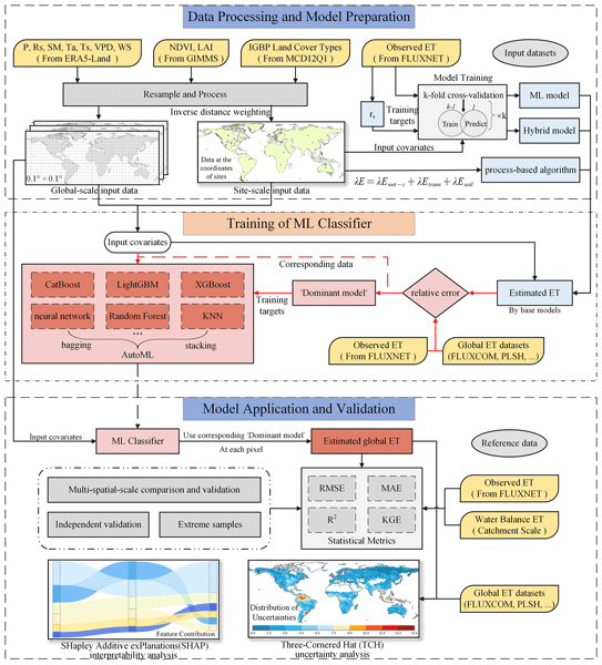
The Classifier-Guided Ensemble model aims to integrate three base models (process-based algorithm, ML-based ET model, and Hybrid model) to optimize the global ET estimation by dividing the ET estimation process into two sub-problems: (a) training a ML classifier to identify the “dominant model” at each pixel, and (b) using the corresponding “dominant model” at each pixel to estimate ET (Fig. 1).

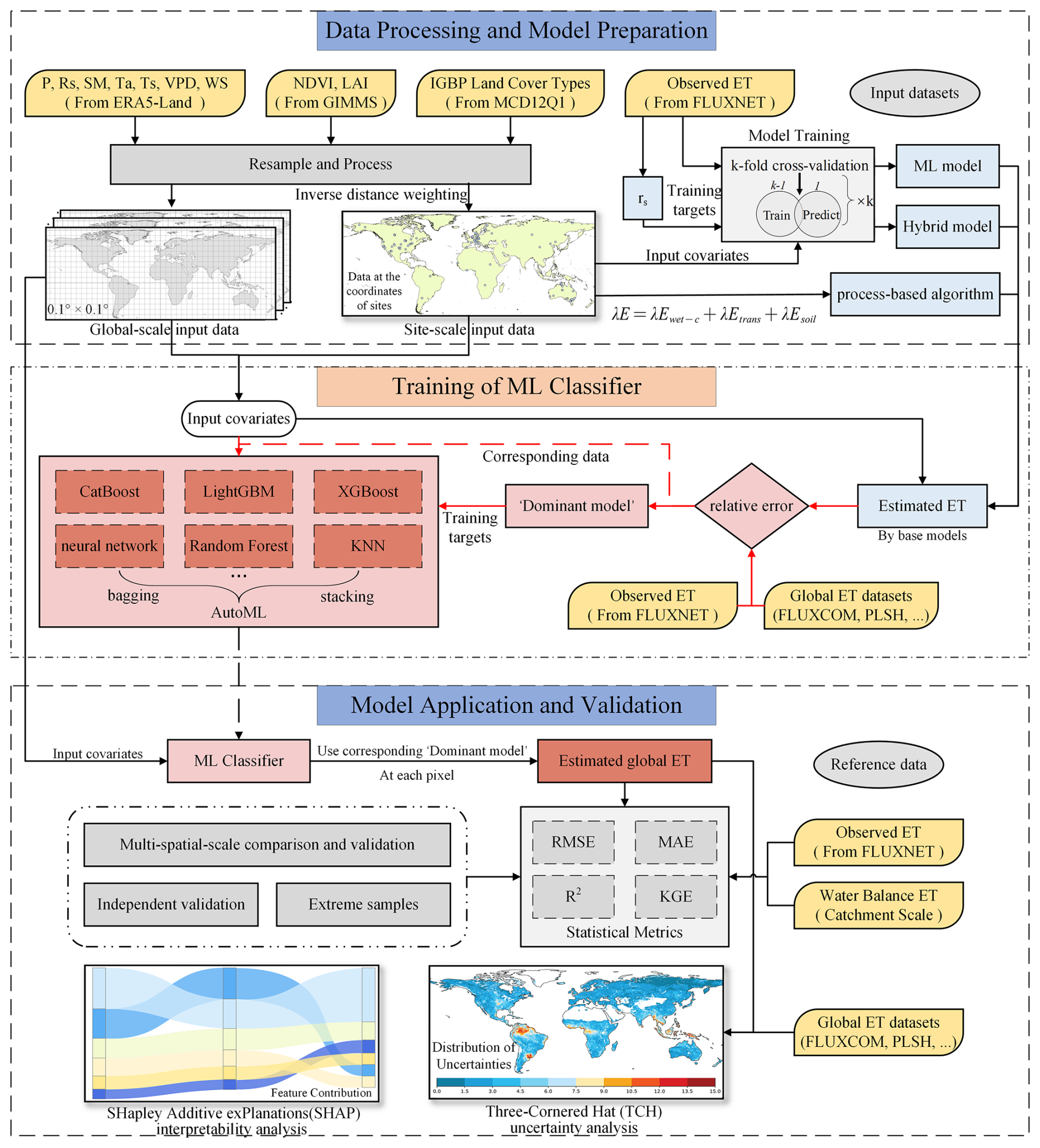
Figure 1 Schematic of the Classifier-Guided Ensemble model. The red arrows indicate the modeling steps of the ML Classifier. P is atmospheric pressure, R_s is incident solar radiation, SM is soil moisture, T_a is air temperature, T_s is soil temperature, VPD is vapor pressure deficit, WS is wind speed, LAI is leaf area index, NDVI is normalized difference vegetation index.

Before training the ML classifier, we needed to first use the three base models to estimate ET at both site and global scales. The estimated ET, in situ ET observations and other global ET products were processed for classification task, in order to obtain the training target. At the site scale, we classified the data at each site for every time point into three types (“ML model-dominated”, “hybrid model-dominated”, and `process-based algorithm-dominated') based on the relative errors between the model-estimated ET and the observed ET. The model with the smallest relative error was the “dominant model” for the corresponding site and time. Specifically, at the site scale, we conducted ten-fold cross-validation on three base models and used ET estimates from the validation sets for classification task, to avoid abnormally high accuracy resulting from model overfitting.

At the global scale, due to the lack of reliable ET observations, we used six widely used global ET products, including FLUXCOM, PLSH, GLEAM a, GLEAM b, GLDAS and ERA5-Land (refer to Sect. 3.3 for details), as references to extract some relatively reliable data for the training dataset. Specifically, we calculated the relative errors between estimated ET of base models and global ET products at each pixel for every time point, obtaining six error values for each base model. If a base model yielded relative errors consistently lower than the other two models across all six products, data of this specific pixel and time point was identified as relatively reliable training data. Data from these specific spatiotemporal points were added into the training data, and the model yielding the lowest relative errors was considered to be the “dominant model” of these specific spatiotemporal points. In contrast, data from the remaining spatiotemporal points were excluded to reduce uncertainty.

In the training phase, we utilized the classification results (i.e., the identified dominant model) as the training target for the ML classifier, using the same input covariates as the other ET models in this study. Through this process, the classifier learned the relationship between input covariates and the dominant model labels. Notably, after the training phase was completed, the classifier could operate independently of ET data. Therefore, during validation and application, we employed the classifier to identify the corresponding dominant model label at each spatiotemporal point based on the input covariates without requiring observed ET data. Subsequently, the identified dominant model at each spatiotemporal point was utilized to generate the ET estimates.

2.5 Other ensemble models used for comparison

We use the Attention-Based ensemble technique used by Liu et al. (2022) as a comparison. The Attention Mechanism is similar to human selective attention and is a method to mimic the human visual and cognitive systems. This technique utilizes the focusing ability of the self-attention mechanism (Zhang et al., 2021), which allows the neural network to focus on what it considers important. It can improve model performance by automatically assigning higher weights to sub-models with higher accuracy. The core formula of this model is as follows:

$$\begin{array}{}\text{(12)}& \begin{array}{rl}{\displaystyle }{f}_{\text{AE}}\left(x\right)& {\displaystyle }={\sum }_{i=\mathrm{1}}^N{\text{Attention}}_i\left(x\right)\\ {\displaystyle }& {\displaystyle }={\sum }_{i=\mathrm{1}}^N{f}_i^{\text{SE}}\left(x\right)\cdot \text{softmax}\left(W_i{f}_i^{\text{SE}}\left(x\right)\right)\\ {\displaystyle }& {\displaystyle }={\sum }_{i=\mathrm{1}}^N{f}_i^{\text{SE}}\left(x\right)\cdot {\displaystyle \frac{\exp \left(W_i{f}_i^{\text{SE}}\left(x\right)\right)}{{\sum }_{i=\mathrm{1}}^N\exp \left(W_i{f}_i^{\text{SE}}\left(x\right)\right)}}\end{array}\end{array}$$

where f_AE(x) is the output of Attention-Based ensemble network, $f_i^{\text{SE}}\left(x\right)$ is the output of ith base model, W_i is attention coefficient, N is the number of base models (N=3 in this study). More detailed algorithm information can be found in Liu et al. (2022).

We used the site-scale ET estimation from three base models as input variables, and ground observed ET as the training target to train a neural network model with attention mechanism which was then used to estimate the global ET as a comparison.

3 Data and model validation

3.1 In situ observations

In this study, we take ground observed surface latent heat flux (LE) to calculate the ET values for training and validation. We used data from 129 flux tower sites (Table A1 and Fig. 2a) in the FLUXNET2015 dataset (https://fluxnet.org/, last access: 24 April 2026) (Pastorello et al., 2020) with the sampling frequency of half-hourly or hourly. These selected sites represent a wide range of major IGBP land cover types: cropland (CRO, 15 sites), deciduous broadleaf forests (DBF, 14 sites), evergreen broadleaf forests (EBF, 10 sites), evergreen needleleaf forests (ENF, 28 sites), grasslands (GRA, 28 sites), mixed forests (MF, 5 sites), open shrublands (OSH, 7 sites), savannas (SAV, 13 sites) and permanent wetlands (WL, 9 sites).

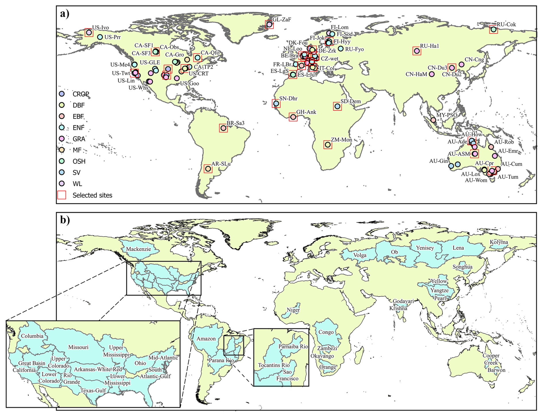
Figure 2 Locations of (a) the 129 Flux sites and (b) the 38 global catchments chosen for analysis in this study. The land cover types are identified based on the International Geosphere-Biosphere Programme (IGBP) biome classification. The red boxes indicate the locations of the 30 sites used in the independent validation.

To mitigate the effects of the uncertainty from data, we only chose the sites with high-quality data and rejected the non-observed data, missing values and data with energy closure less than 70 % in the original dataset. Due to potential issues with eddy covariance technology and measurements under rainy conditions (Medlyn et al., 2011), we excluded rainy day samples to avoid errors. We also applied the Bowen ratio closure method to address the issue of energy imbalance in original observations (Foken, 2008; Twine et al., 2000). If the filtered data had more than 20 % missing values in a month, the data for that month was removed. The remaining data were then processed using linear interpolation and averaging to generate monthly-scale data.

3.2 Catchment-scale ET

At the catchment scale, the water balance method can be used to obtain a more reliable ET data (Pascolini-Campbell et al., 2020). The catchment-scale ET can be calculated as:

$$\begin{array}{}\text{(13)}& \text{ET}=P-Q-{\displaystyle \frac{\mathrm{d}S}{\mathrm{d}t}}\end{array}$$

where P is precipitation, Q is runoff at the basin outlet, and $\mathrm{d}S/\mathrm{d}t$ is the change in total water storage. We used the dataset of the water-balance-based evapotranspiration of global typical large river basins published by Ma et al. (2024). This dataset spans a 34 year period from 1983–2016 and can be downloaded from the National Tibetan Plateau Data Center (Ma, 2024). This data is derived from water balance methods combined with four different precipitation data sources (P), three types of terrestrial water storage change estimates ($\mathrm{d}S/\mathrm{d}t$) and observed flow data from control sites (Q). We selected 38 major catchments (>200 000 km²) in this dataset as our validation data (Fig. 2b and Table A2).

3.3 Global- scale datasets

At the global scale, given the current lack of reliable direct global ET observations for validation, we collected six widely used ET products derived from diverse data sources, forcing data, and calculation methods to conduct a comprehensive validation. (1) FLUXCOM (Jung et al., 2019; Tramontana et al., 2016) provides a latent heat dataset, with 0.0833°×0.0833° resolution and time spanning a 75 year period from 1950 onwards generated, from energy flux measurements from FLUXNET eddy covariance towers and meteorological data utilizing only machine learning methods. (2) Process-based Land Surface Evapotranspiration/Heat Fluxes (PLSH) (Zhang et al., 2015) is a product with 0.0833°×0.0833° resolution and time spanning a 32 year period from 1982–2013. The dataset is driven by satellite observations of photosynthetic canopy cover and surface meteorology inputs. (3) Global Land Evaporation Amsterdam Model (GLEAM) version 3.8a (Martens et al., 2017; Miralles et al., 2011) is an established ET product based on satellite and reanalysis data with 0.25°×0.25° resolution and time spanning the 44 year period from 1980–2022. (4) GLEAM version 3.8b (Martens et al., 2017; Miralles et al., 2011) is also selected because of its different forcing data. It is based on only satellite data with 0.25°×0.25° resolution and time spanning the 20 year period from 2003–2022. (5) Global Land Data Assimilation System (GLDAS) version 2.1 (Rodell et al., 2004; Beaudoing and Rodell, 2020), a product with 0.25°×0.25° resolution and time spanning a 24 year period from 2001 onwards, is generated by combining data assimilation techniques with satellite and ground-based observations. (6) European Centre for Medium-range Weather Forecasts (ECMWF)-ERA5-Land product (Muñoz Sabater, 2019) is a reanalysis product based on multi-source data with 0.1°×0.1° and time spanning a 75 year period from 1950 onwards.

Input covariates for all models described in Sect. 2 were derived from the same source to ensure consistency in the training process. In the input training data, variables P, R_s, SM, ST, T_a, VPD, WS are sourced from the ERA5-land product. Since the ERA5-Land dataset only provides dew point temperature data, we used the following formula for calculation (Abbott and Tabony, 1985):

$$\begin{array}{}\text{(14)}& \text{VPD}=\mathrm{0.6108}\left[{\mathrm{e}}^{\frac{\mathrm{17.27}T}{T+\mathrm{237.3}}}-{\mathrm{e}}^{\frac{\mathrm{17.27}{T}_{\mathrm{d}}}{T_{\mathrm{d}}+\mathrm{237.3}}}\right]\end{array}$$

Here, T and T_d represent temperature and dew point temperature respectively (°C). Although these data are also available in the in situ observations, we chose to use the global-scale dataset instead to avoid issues caused by inconsistencies in spatial scales between the training data and the calculation data (Xiao et al., 2008). We employed an inverse distance weighting method to extract data at the coordinates of the corresponding sites for training data.

Other variables LAI and NDVI are sourced from the Global Inventory Modeling and Mapping Studies (GIMMS) NDVI and LAI products (Cao et al., 2023; Li et al., 2023), which are half-month products with 0.0833°×0.0833° resolution. We averaged the two values for the month to obtain the monthly average data. The IGBP variables are sourced from the MODIS Land Cover Climate Modeling Grid Product (MCD12C1) (Friedl and Sulla-Menashe, 2015), which is a spatially aggregated and reprojected version of the tiled MCD12Q1 product with 0.05°×0.05° resolution. We resampled all these data to 0.1° spatial resolution, the same as the ERA5-Land product that contains the most input variables.

3.4 Model validation

3.4.1 Site and catchment scale validation

Given that both in situ observations and the total catchment ET calculated by the water balance method are relatively reliable datasets, we can directly compare the ET generated by our model with these datasets at site and catchment scale. At the site scale, we conducted k-fold cross-validation with k=10. In each fold we selected 10 % of the data at each site as the validation set and the remaining data as the training set. In addition, we carried out independent validation by selecting 30 independent sites excluded from the training data (Table A3 and Fig. 2a) to evaluate the spatial simulation performance of our Classifier-Guided Ensemble model. The selected independent validation sites cover multiple land cover types and most of the major regions. Also, we evaluated the ET estimation performance of our model on extreme samples sorted in ascending order within the 0th–1st percentiles and 99th–100th percentiles for six variables (LAI, NDVI, R_s, SM, T_a, VPD) to verify the extrapolation performance of the model. At the catchment scale, we used calculated catchment ET to compare with the total catchment ET estimated by our model and other global ET products.

To quantitatively validate the performance of our model, we used several statistical metrics: Root Mean Squared Error (RMSE), Mean Absolute Error (MAE), Coefficient of Determination (R²), and Kling–Gupta Efficiency (KGE) (Table 1). MAE and RMSE are used to measure the closeness between the model results and observations. R² can be used to assess the correlations. KGE comprehensively considers the relative error, correlation coefficient and variance of the model results, providing a comprehensive assessment of the model's overall performance.

Table 1 The explanation of statistical metrics used to evaluate model performance in this study. n/a: not applicable.

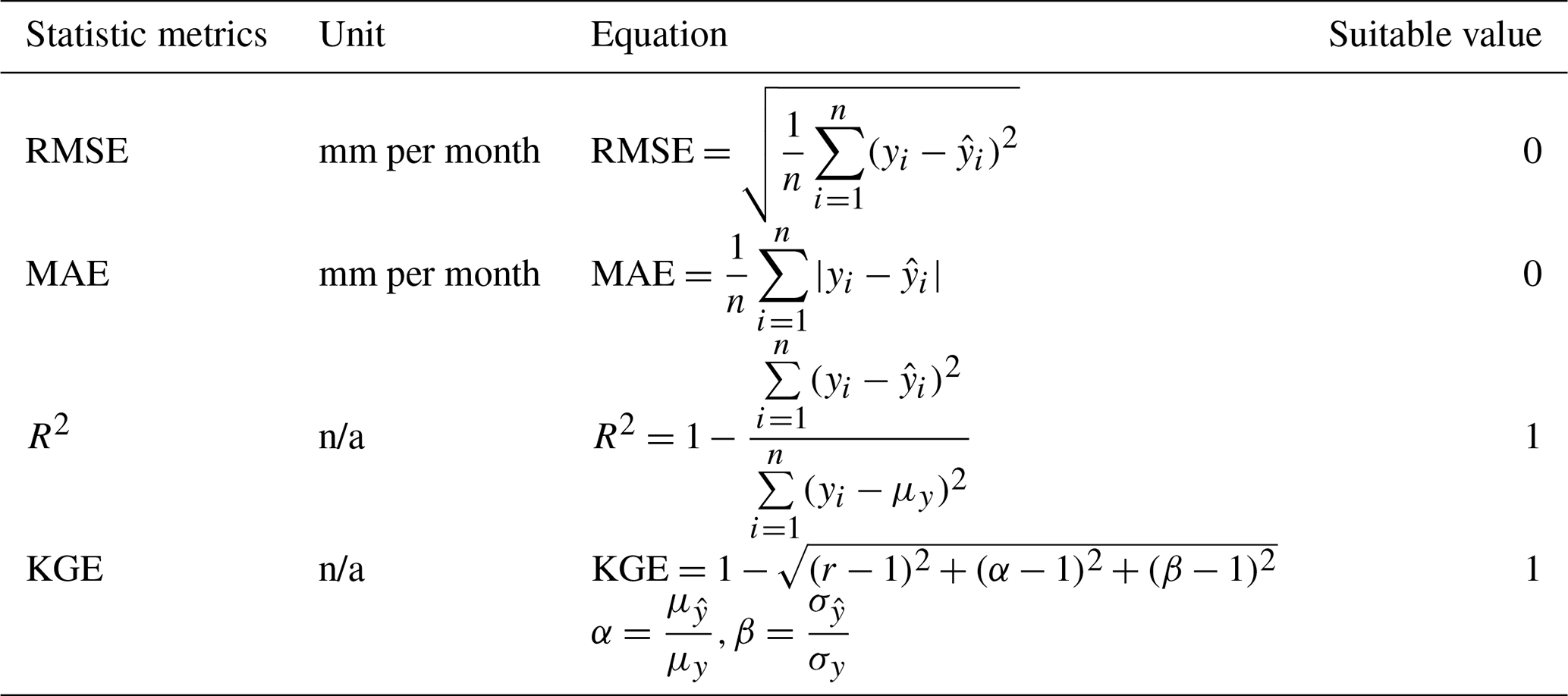
Note: y_i and ${\widehat{y}}_i$ represent observations and estimations, respectively, α is the bias ratio, β is the variability ratio, σ represents the standard deviation, μ represents the average.

3.4.2 Global scale validation

Taking into account the available years of each product, we analyzed the data for the period from 2003–2013, with the data of 2003 and 2004 serving as the training set and the data of remaining years as the validation set. At global scale, due to the lack of reliable ET observations, conventional validation methods are not feasible. Therefore, we used the three-cornered hat (TCH) method (Tavella and Premoli, 1994) to quantify the uncertainties of ET estimation. TCH is a reliable method for estimating the uncertainty of various time series products and has been used for validation of multiple datasets (Liu et al., 2021). We used the same formula as in (Xie et al., 2024). The time series of ET at each pixel can be expressed as:

$$\begin{array}{}\text{(15)}& X_k=X_{\mathrm{t}}+{\mathit{\epsilon }}_k,\forall k=\mathrm{1},\mathrm{2},\mathrm{3},\mathrm{\dots },N\end{array}$$

where k represents the index of the corresponding ET product, N is the total number of ET products included in the validation, X_t represents the true value and ε_k represents the error term.

The truth value of ET cannot be obtained, so we need to get the ε_k without X_t. To solve this problem, the TCH algorithm defines a product as a reference product to get a matrix Y_k,m as:

$$\begin{array}{}\text{(16)}& Y_{k,m}=X_k-X_{\mathrm{R}}={\mathit{\epsilon }}_k-{\mathit{\epsilon }}_{\mathrm{R}},\forall k=\mathrm{1},\mathrm{2},\mathrm{3},\mathrm{\dots },N-\mathrm{1}\end{array}$$

where X_R is the arbitrarily selected reference product, Y_k,m is an $M\times (N-\mathrm{1})$ matrix, M is the length of the time series of X. S, the covariance matrix of Y, is related to the unknown M×N covariance matrix of the individual noise Q as (Galindo and Palacio, 2003):

$$\begin{array}{}\text{(17)}& {\displaystyle }& {\displaystyle }S=J\cdot Q\cdot J^{\mathrm{T}}\text{(18)}& {\displaystyle }& {\displaystyle }{J}_{N-\mathrm{1},N}=\left(\begin{array}{ccccc}\mathrm{1}& \mathrm{0}& \mathrm{\cdots }& \mathrm{0}& -\mathrm{1}\\ \mathrm{0}& \mathrm{1}& \mathrm{\cdots }& \mathrm{0}& -\mathrm{1}\\ \mathrm{⋮}& \mathrm{⋮}& \mathrm{⋮}& \mathrm{⋮}& \mathrm{⋮}\\ \mathrm{0}& \mathrm{0}& \mathrm{0}& \mathrm{\cdots }& -\mathrm{1}\end{array}\right)\end{array}$$

Since the number of equations is still less than the number of unknowns, it is impossible to solve the equation. They used the Kuhn–Tucker theorem proposed by Galindo and Palacio (1999) to solve the constrained minimization problem. The definition of the objective function and constraint function is:

$$\begin{array}{}\text{(19)}& {\displaystyle }& {\displaystyle }{F}_{(r_{\mathrm{1}N},\mathrm{\dots },r_{NN})}=-{\displaystyle \frac{\mathrm{1}}{K^{\mathrm{2}}}}\cdot {\sum }_{i<j}^N{r}_{ij}^{\mathrm{2}}\text{(20)}& {\displaystyle }& {\displaystyle }{H}_{(r_{\mathrm{1}N},\mathrm{\dots },r_{NN})}=-{\displaystyle \frac{\left|Q\right|}{\left|S\right|\cdot K}}<\mathrm{0}\end{array}$$

where $r_{\mathrm{1}N},\mathrm{\dots },r_{NN}$ are the elements of the corresponding Q. They also used the initial conditions for the iteration proposed by Torcaso et al. (1998):

$$\begin{array}{}\text{(21)}& {\displaystyle }& {\displaystyle }{r}_{iN}^{\mathrm{0}}=\mathrm{0},i<N;\text{(22)}& {\displaystyle }& {\displaystyle }{r}_{NN}^{\mathrm{0}}={\displaystyle \frac{\mathrm{1}}{\mathrm{2}\cdot S^{\ast }}},S^{\ast }=[\mathrm{1},\mathrm{\dots },\mathrm{1}]\cdot S^{-\mathrm{1}}\cdot (\mathrm{1},\mathrm{\dots },\mathrm{1}{)}^{\mathrm{T}}\end{array}$$

Finally, the Q value is obtained by minimizing the objective function. More detailed information can be found in their paper (Galindo and Palacio, 1999, 2003; Torcaso et al., 1998; Xie et al., 2024).

3.4.3 ML model interpretability analysis

We used SHAP (SHapley Additive exPlanations) to analyze the interpretability of the ML classifier we used. SHAP was originally proposed in game theory (Shapley, 1952) and was used as a method to equitably distribute benefits by calculating each member's marginal contribution. Subsequently, it was used to compute the marginal contribution of each input variables to enhance the interpretability of machine learning (Lundberg and Lee, 2017).

The Python library of SHAP was used to calculate the SHAP values for each input feature. SHAP library is applicable for interpretability analysis of ensemble models that integrate multiple ML models. In this study, SHAP values were employed to enhance our understanding of how our ML classifier selects the “dominant model”.

4 Results

4.1 Model evaluation with in situ observations

4.1.1 Model Evaluation using EC observations

To evaluate the model simulation performance, we conducted a ten-fold cross-validation at all selected EC sites (Fig. 3). First, we check whether the integrated base models could accurately estimate ET at site scale (Fig. 3b, c and e). It is found that both ML model and Hybrid model perform well with R² and KGE nearing 0.9, ensuring the reliability of ensemble model while process-based algorithm exhibits relatively lower performance, with a KGE of 0.65, R² of 0.48, MAE of 17.41 mm per month, RMSE of 26.45 mm per month. Despite the lower accuracy of process-based algorithm at site scale, it is also integrated as the employed physically-founded equations enable process-based algorithm to maintain acceptable performance in data-sparse regions.

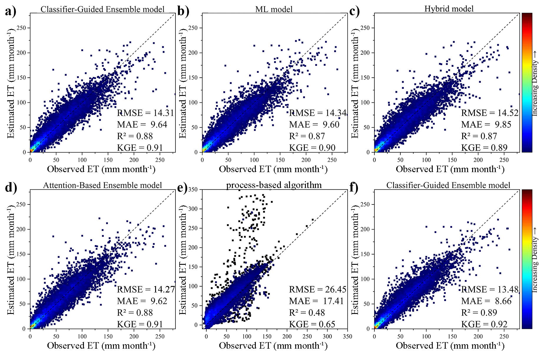
Figure 3 Performance of (a) Classifier-Guided Ensemble model, (b) ML model, (c) Hybrid model, (d) Attention-Based Ensemble model, (e) process-based algorithm and (f) Classifier-Guided Ensemble model (enhanced by additional global-scale training data) in ten-fold cross-validation.

The performance of our Classifier-Guided Ensemble model and the model with more training data are shown in Fig. 3a and f. Although when trained using only site-scale data, our Classifier-Guided Ensemble model performs well with a KGE of 0.91, R² of 0.88, MAE of 9.64 mm per month, RMSE of 14.31 mm per month, showing clear advantages over base models, it cannot significantly outperform the Attention-Based Ensemble model with the same KGE and R², lower RMSE of 14.27 mm per month and lower MAE of 9.62 mm per month (Fig. 3d). As illustrated in Fig. 3e, the process-based algorithm exhibits inferior performance to data-driven models at the site scale, resulting in its near exclusion from the classifier when trained only on in situ observations. Expanding the training dataset with global datasets enables the classifier to better recognize the scenarios where each base model performs best, with accuracy improving from 70 %–90 %, particularly for process-based algorithm. Therefore, our model can achieve the best performance among all of the models used for comparison in the validation dataset, with a KGE of 0.92, R² of 0.89, MAE of 8.66 mm per month, RMSE of 13.48 mm month−1.

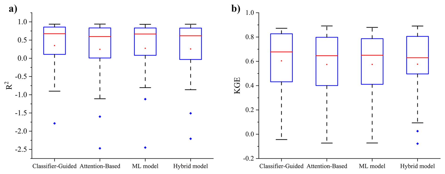
Figure 4 The (a) R² and (b) KGE of the Classifier-Guided Ensemble model, Attention-Based Ensemble model, ML model, and Hybrid model in independent validation. The red lines represent the median of the validation metrics, and the red dots represent the average values of the validation metrics.

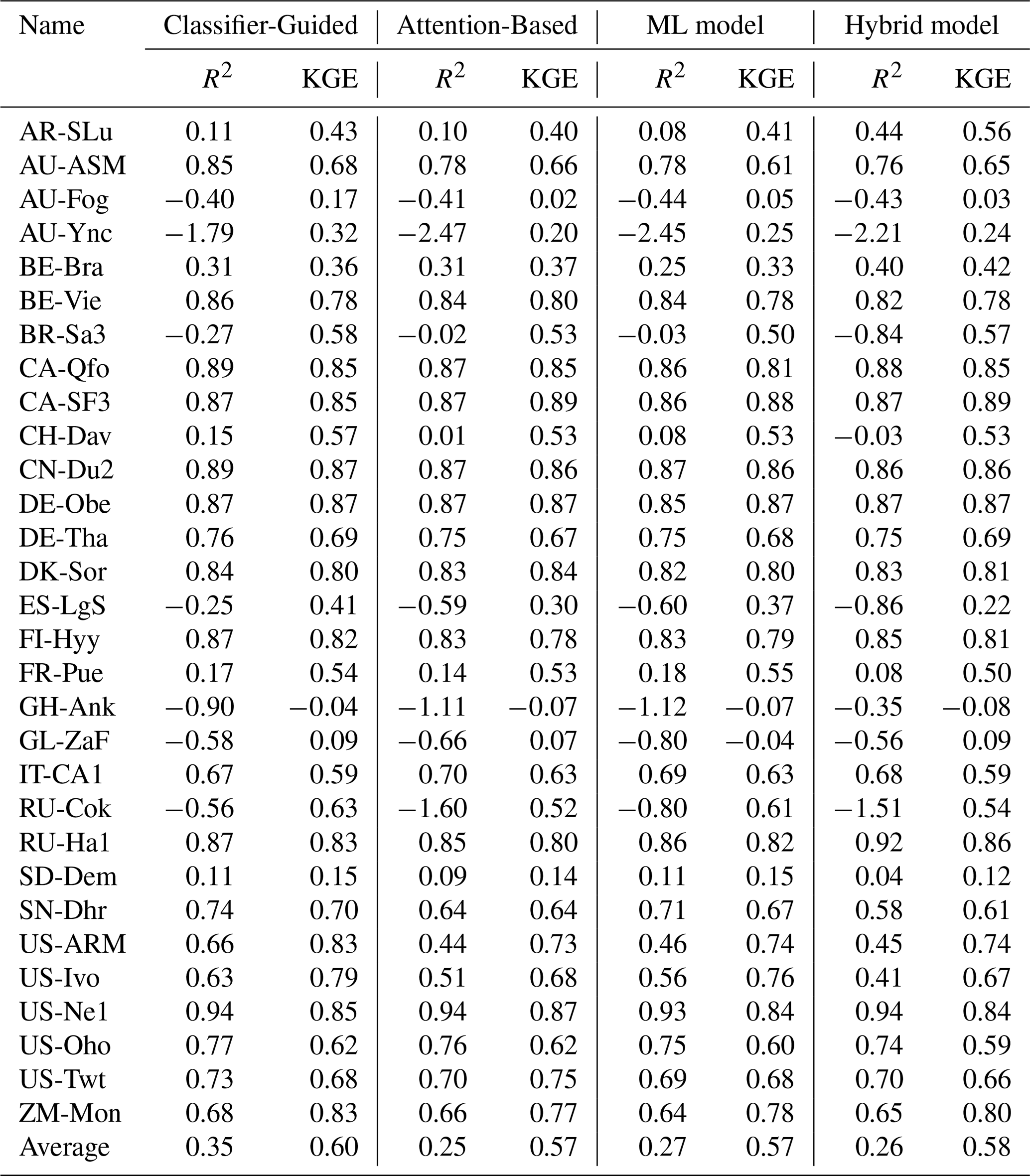
The independent validation results shown in Fig. 4 and Table A4 also indicate that our model exhibits excellent generalizability in these independent sites. The ET estimation from Classifier-Guided Ensemble model achieves the best performance among all compared models, with a higher average R² of 0.35 and a higher average KGE of 0.60. The Classifier-Guided Ensemble model performs well in most of the selected independent sites, especially at the CH-Dav and US-ARM sites, as it can make better use of the process-based algorithm's extrapolation strengths, yielding better outcomes even when ML model and Hybrid model struggle, while the Attention-Based Ensemble model's results are closer to those of the ML model at most sites, resulting in poorer performance in independent validation.

The results from the k-fold cross-validation and independent validation indicate that our Classifier-Guided Ensemble model performs well in estimating ET at site scale, exhibiting better stability and generalizability, and the inclusion of global-scale data makes our model perform better.

4.1.2 Model Evaluation under different sites and vegetation cover conditions

In situ observations were also used to evaluate the performance of models across different sites and land cover types, thereby validating the models' spatial simulation performance. The Taylor diagram is used to compare the performance of the models, where the two axes represent the root mean square error (RMSE, in mm per month), and the curves indicate the Pearson's correlation coefficient (r).

As Fig. 5a and Table 2 demonstrates, Classifier-Guided Ensemble model performs the best among the four models in the majority of the site, with lower average RMSE of 14.55 mm per month (Attention-Based Ensemble model: 15.41 mm per month, Hybrid model: 15.52 mm per month, ML model: 15.46 mm per month), and higher average correlation coefficient (r) of 0.90 (Attention-Based Ensemble model: 0.88, Hybrid model: 0.88, ML model: 0.87). Specifically, the best-performing sites for multiple models include “CA-Obs” (RMSE: Classifier-Guided Ensemble model: 3.92 mm per month, Attention-Based Ensemble model: 3.91, Hybrid model: 5.27 mm per month, ML model: 3.90 mm per month) and “CA-SF1” (RMSE: Classifier-Guided Ensemble model: 3.75 mm per month, Attention-Based Ensemble model: 4.83 mm per month, Hybrid model: 4.08 mm per month, ML model: 5.75 mm per month). Furthermore, Classifier-Guided Ensemble model significantly outperformed the other models at “US-Me4” and “DE-Zrk”, achieving RMSE below 4.0, whereas all other models exceeded 8.0 at these sites.

Table 2 Performance of different ET models as indicated by averaged RMSE and R² for all sites, based on the cross-validation dataset.

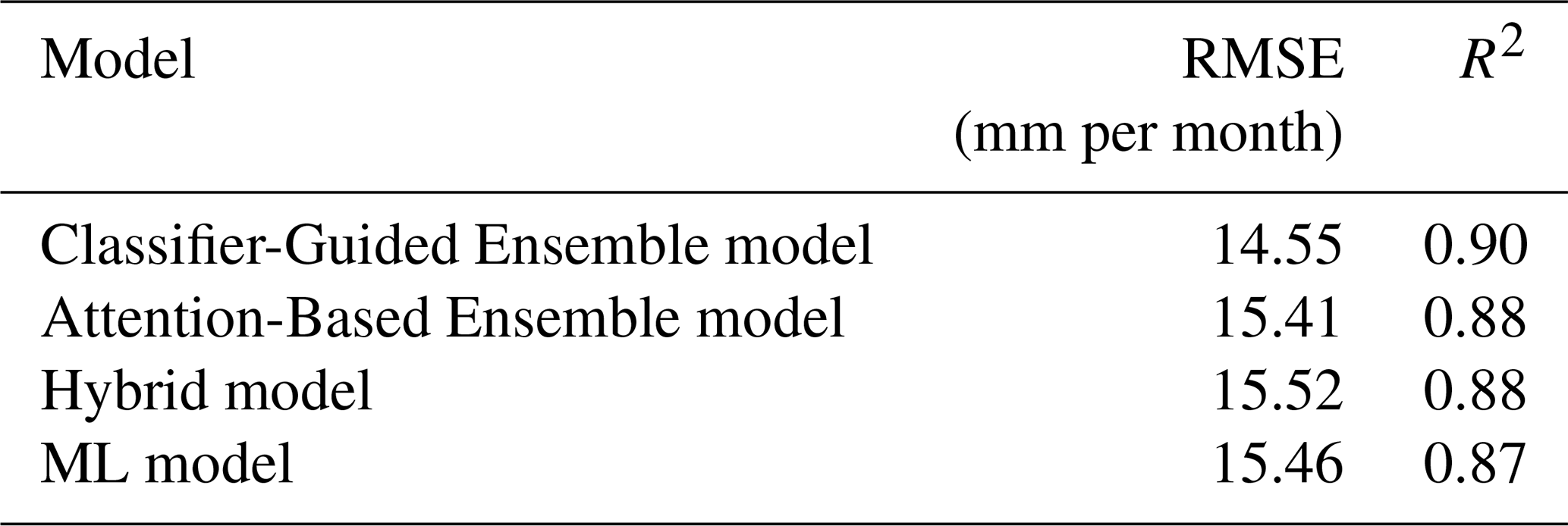
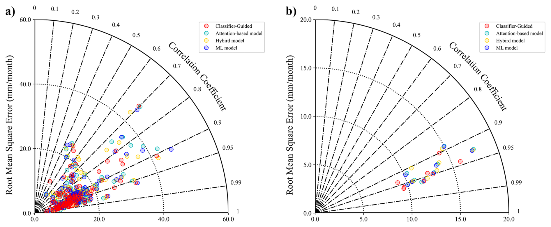
Figure 5 Taylor diagram that compares the performance of the four models with ground observations for (a) different sites and (b) different land cover types, based on the cross-validation dataset.

Classifier-Guided Ensemble model also demonstrates greater performance than the other three models in the majority of land cover types (Fig. 5b and Table 3), with lower average RMSE of 16.88 mm per month (Attention-Based Ensemble model: 17.40 mm per month, Hybrid model: 17.38 mm per month, ML model: 17.94 mm per month), and higher average correlation coefficient (r) of 0.93 (Attention-Based Ensemble model: 0.92, Hybrid model: 0.93, ML model: 0.92). Classifier-Guided Ensemble model outperforms other models across most land cover types, with the exception of the CSH, where its performance is slightly inferior to Attention-Based Ensemble model and Hybrid model. For CSH, the limitation to a single site (“US-ZS2”) with sparse data resulted in lower accuracy for all models. In this specific case, although Classifier-Guided Ensemble model yielded better results than both the ML model and the Attention-Based Ensemble model, it did not outperform the Hybrid model.

Table 3 Performance of different ET models as indicated by RMSE and R² for all IGBP land cover types, based on the cross-validation dataset.

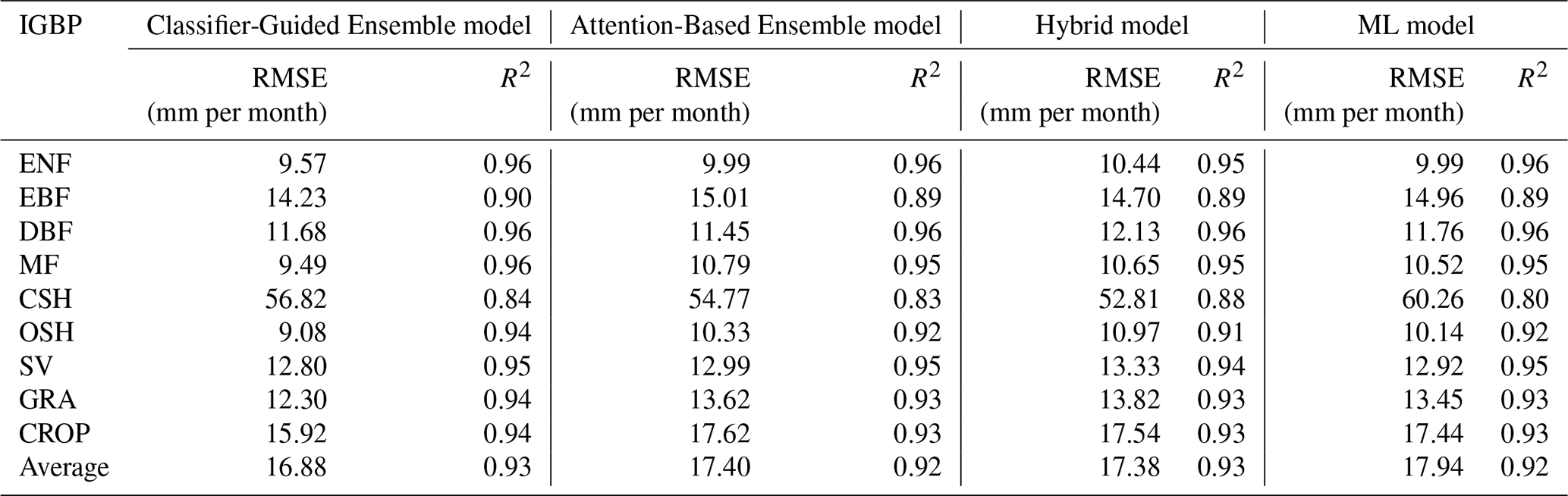
Further, we notice that the Attention-Based Ensemble model assigns more “attention” to the ML model, since the ML model performs best at the site scale among the three base models. Therefore, the Attention-Based Ensemble model yields results similar to the ML model across sites and land cover types, and at certain sites, such as “CA-SF1”, the Attention-Based Ensemble model is significantly outperformed by the Hybrid model, while Classifier-Guided Ensemble model can fully utilize the characteristics of the base models and get better results, which is consistent with the conclusion from independent validation. In summary, the proposed model better fits the data from different sites and different land cover types, which demonstrates the effectiveness of our ensemble method.

4.1.3 Model Evaluation using extreme samples

In order to verify the extrapolation performance of the models for extreme samples, we compared the performance of these models for multiple extreme samples. The heatmaps in Fig. 6 indicate that for the majority of these extreme samples, our Classifier-Guided Ensemble model can accurately estimate ET.

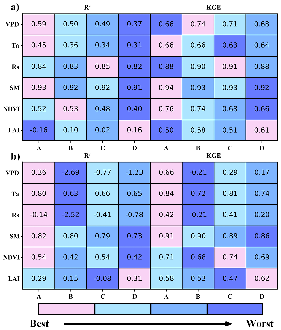
Figure 6 The comparison of different models (A Classifier-Guided Ensemble model, B Attention-Based Ensemble model, C ML model, D Hybrid model) under extreme conditions in the form of heatmaps. (a) and (b) represent the extreme samples sorted in ascending order within the 0th–1st percentiles and 99th–100th percentiles, respectively.

For the 99th–100th percentiles of the VPD in particular, Classifier-Guided Ensemble model performs significantly better than the other models, with a KGE of 0.66, R² of 0.36, while the KGE of other models is below 0.3 and the R² is less than 0. This shows that Classifier-Guided Ensemble model has the potential to efficiently select the “dominant model” to achieve good results even when these existing ML models perform poorly. Under the cases of high T_a, high R_s and low T_a, Classifier-Guided Ensemble model performs significantly better than the other models. Only under the three cases of low VPD, low R_s and low LAI, Classifier-Guided Ensemble model is not as good as the other models and the difference is not significant, with the KGE being 0.08, 0.02 and 0.08 lower than that of the Attention-Based Ensemble model, respectively. In most extreme cases, Classifier-Guided Ensemble model can yield stronger extrapolation performance than individual base models or other ensemble models, providing more accurate ET estimates under extreme weather events.

4.2 Model evaluation at catchment scale

To validate the model performance for the catchment-scale application, we used six ET products, Classifier-Guided Ensemble model, and Attention-Based Ensemble model to estimate ET in each catchment and compare them to the water balance ET dataset. The results show that Classifier-Guided Ensemble model performs better than other comparison models and products (Fig. 7), with a KGE of 0.94, R² of 0.92, MAE of 6.17 mm per month, RMSE of 7.73 mm per month and the slope of the regression of estimated ET versus water balance ET for our model (0.99) is closer to 1 than that of the other ET products and models. The Attention-Based Ensemble model also performs better than most of the ET products used, with a KGE of 0.89, but the results are not as good as those of our model, ERA5-Land, and GLDAS ET products as it exhibits higher RMSE and MAE. This proves that our model is in better agreement with the catchment water balance ET.

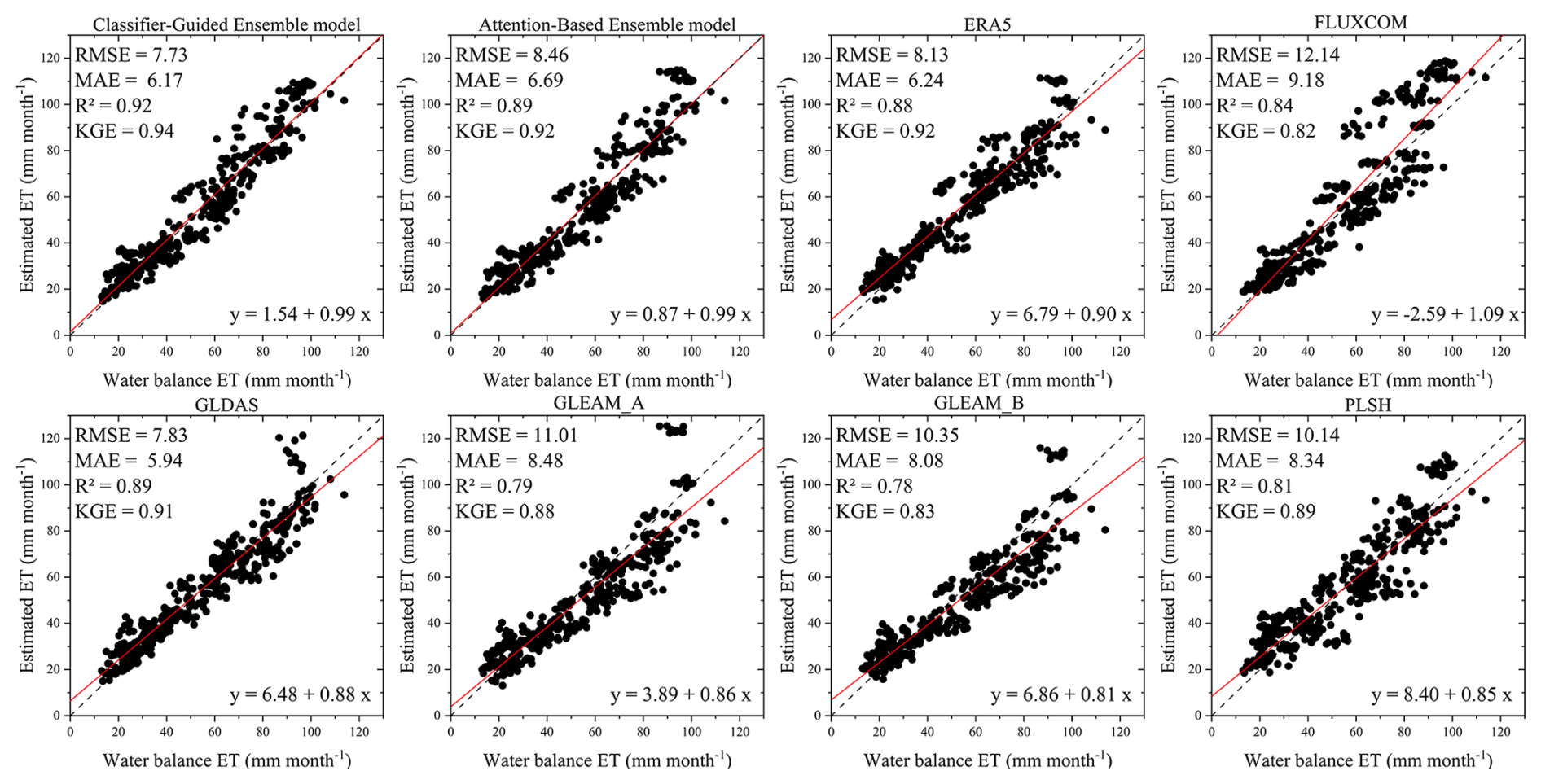
Figure 7 Scatterplot for the relationship between estimated ET and water balance ET (each point represents a catchment over a one-year period).

The spatial distribution of RMSE across 38 catchments (Fig. 8) further demonstrate the superior performance of our model. Compared to the Attention-Based Ensemble model, our model shows significant improvement in RMSE for catchment “Mackenzie”, “Rio Grande”, “Lower Colorado”, “Amazon”, “Kolyma ”, “Godavari”, “Krishna”, “Orange”, “Cooper Creek” and “Barwon”, with a reduction in RMSE of over 20 %. Especially in catchment “Godavari”, the RMSE of our model is 5.59 mm per month and the RMSE of Attention-Based Ensemble model is 12.02 mm per month, with a difference of more than 50 %. In some other catchments (“Mid-Atlantic”, “Ohio”, “Upper Colorado”, “Ob” and “Yellow”), the RMSE of the Attention-Based Ensemble model is over 20 % lower than that of our model. Compared to another well-performing GLDAS product, there are large differences between our model and GLDAS due to the difference in calculation methods, with each of these two methods having lower RMSE in 19 catchments. In summary, while there are some differences in ET estimation among our model, the Attention-Based Ensemble model, and other products in different catchments, our model is in better agreement with the catchment water balance ET in the majority of catchments.

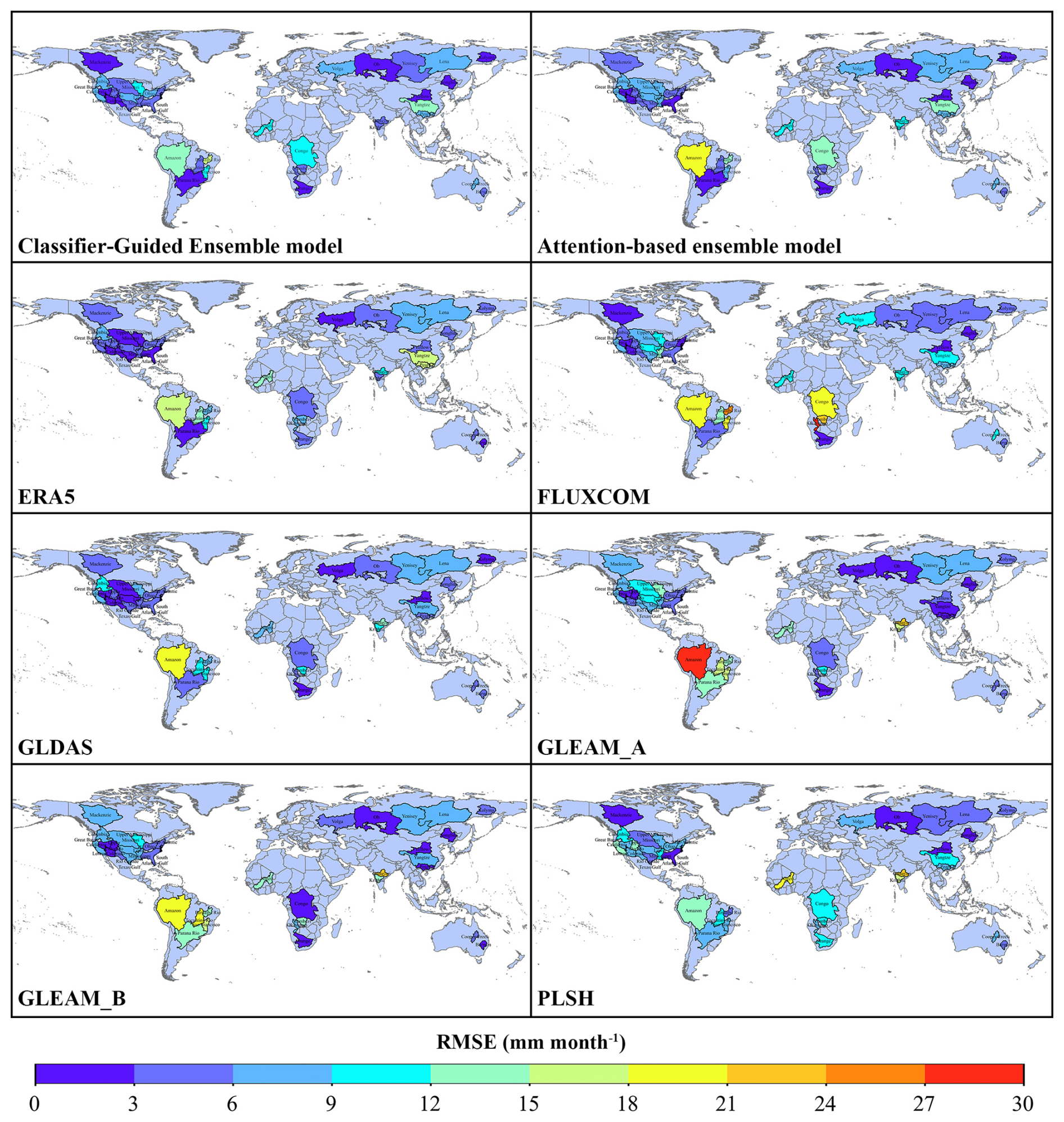
Figure 8 Distributions of the root-mean-square error (RMSE) for the 38 catchments.

4.3 Model evaluation at global scale

To further validate the performance of our model on larger spatial scales, we compared the multi-year average ET estimated by Classifier-Guided Ensemble model and Attention-Based Ensemble model, and other ET products. We primarily compared our Classifier-Guided Ensemble model with Attention-Based Ensemble model to validate the performance of our ensemble method and with FLUXCOM, which is an ET product generated based on pure ML models, to evaluate the differences between ensemble model and pure ML models. Additionally, other ET products were included as reference for the analysis. Some ET products, like FLUXCOM, contain missing values in certain regions, and these regions were excluded from the comparison.

4.3.1 Evaluation of multi-year average ET estimates

Figure 9 shows the spatial distribution of the multiyear (2005–2013) mean global ET estimates for the ET models and products. Our Classifier-Guided Ensemble model shows expected global patterns of ET and all of these ET models and products generally show similar spatial pattern. ET values are relatively higher in mid-latitude regions near the equator, including the Amazon Basin, the Congo Basin, and Southeast Asia, while lower ET values are shown in some arid regions, including the Sahara Desert and Central Asia, as well as in high-latitude alpine regions, including northern Russia, and northern Canada. The multiyear mean ET ranges from 46.99–49.69 mm per month, with FLUXCOM having the highest average ET and GLEAM_B having the lowest average ET.

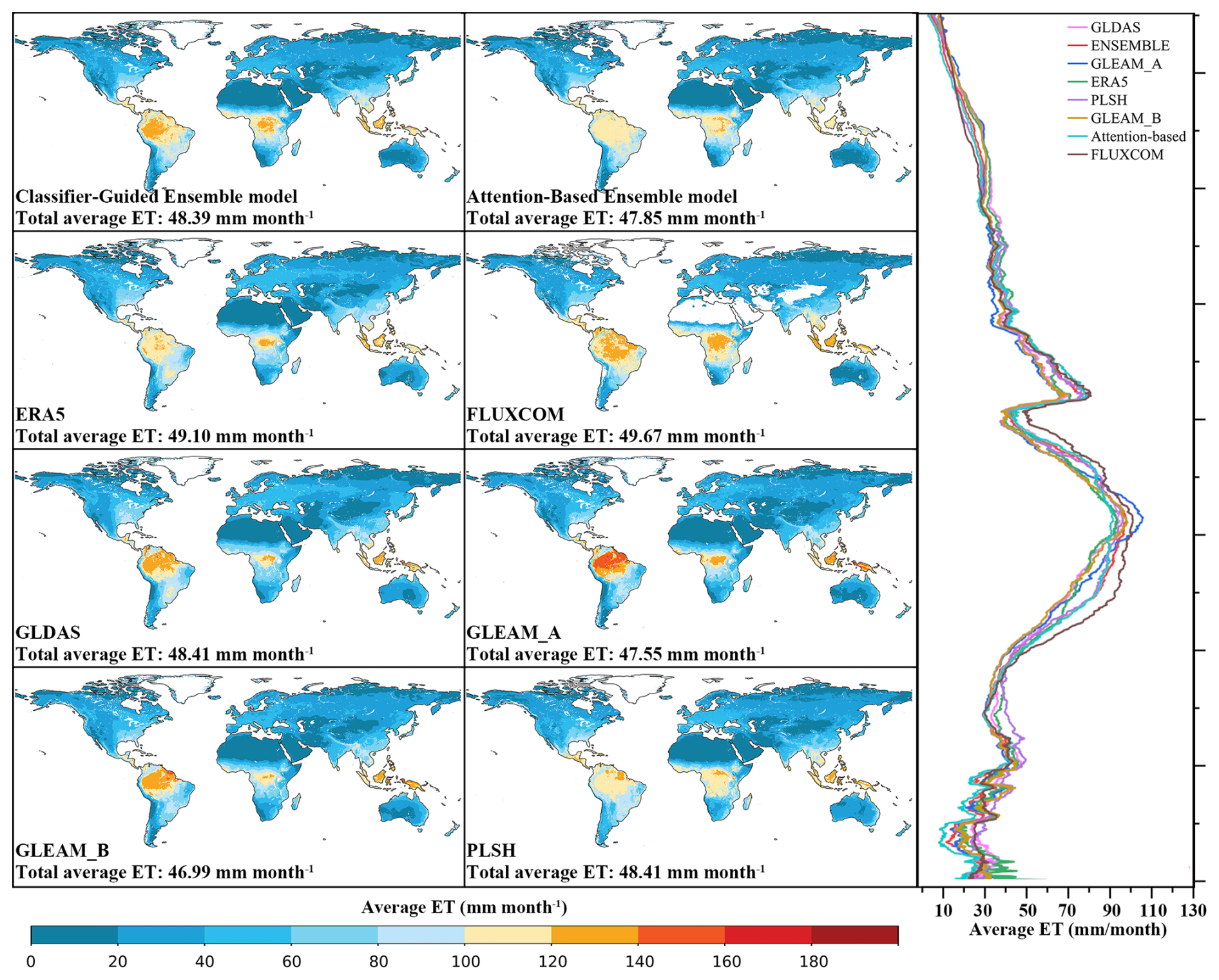
Figure 9 Average annual land evapotranspiration from 2005–2013 for Classifier-Guided Ensemble model, Attention-Based Ensemble model and other ET products. The latitudinal profiles of these datasets are shown in the right panel.

Despite their great consistency in spatial patterns, there are still some regional discrepancies detected among these datasets. Compared with other products, the Attention-Based Ensemble model shows the largest discrepancy in tropical regions, as it provides lower ET estimates, with almost no regions exhibiting ET exceeding 120 mm per month. This may be attributed to the ML model's limited ability to estimate extreme high values, as well as the potential underestimation of ET by the ensemble model (Cai et al., 2024). Compared with the Attention-Based Ensemble model, our Classifier-Guided Ensemble model shows better spatial consistency with other ET products and avoids the underestimation of high values. The latitudinal average ET distribution for each dataset also confirms this conclusion. The Attention-Based Ensemble model shows lower ET estimates in both high-ET and low-ET regions and the FLUXCOM product tends to overestimate ET in low-latitude regions, particularly in areas slightly below the peak values, while the ET profile estimated by our model shows improvement in these areas. Overall, our model generally performs well and provides a reasonable global ET estimate, indicating a distinct improvement in generalizability with the introduction of ML classifier.

4.3.2 Uncertainty analysis at global scale

The proposed model also demonstrates strong stability in the uncertainty analysis. Figure 10 illustrates the uncertainty distribution estimated from the TCH method for eight global ET estimates during the period from 2005–2013. All of these datasets exhibit high stability, with less than 5 mm per month mean uncertainty in most areas. The lowest mean uncertainty is achieved by Classifier-Guided Ensemble model (1.45), followed by FLUXCOM (1.54), Attention-Based Ensemble model (1.63), GLEAM_A (1.84), GLEAM_B (1.88), PLSH (1.93), ERA5 (2.25), GLDAS (3.08). The uncertainty distribution of these datasets also shows a similar spatial pattern and typically high uncertainty is found in low-latitude areas. Many studies have investigated the uncertainty of these ET products. Xie et al. (2024) used the TCH method to assess the uncertainty of several products from 2003–2015 and found that FLUXCOM had the lowest uncertainty. Zhu et al. (2022) and Li et al. (2022) also evaluated several products and found that the GLEAM product exhibited lower uncertainty. The uncertainty of these products we calculated is consistent with the results of these previous studies.

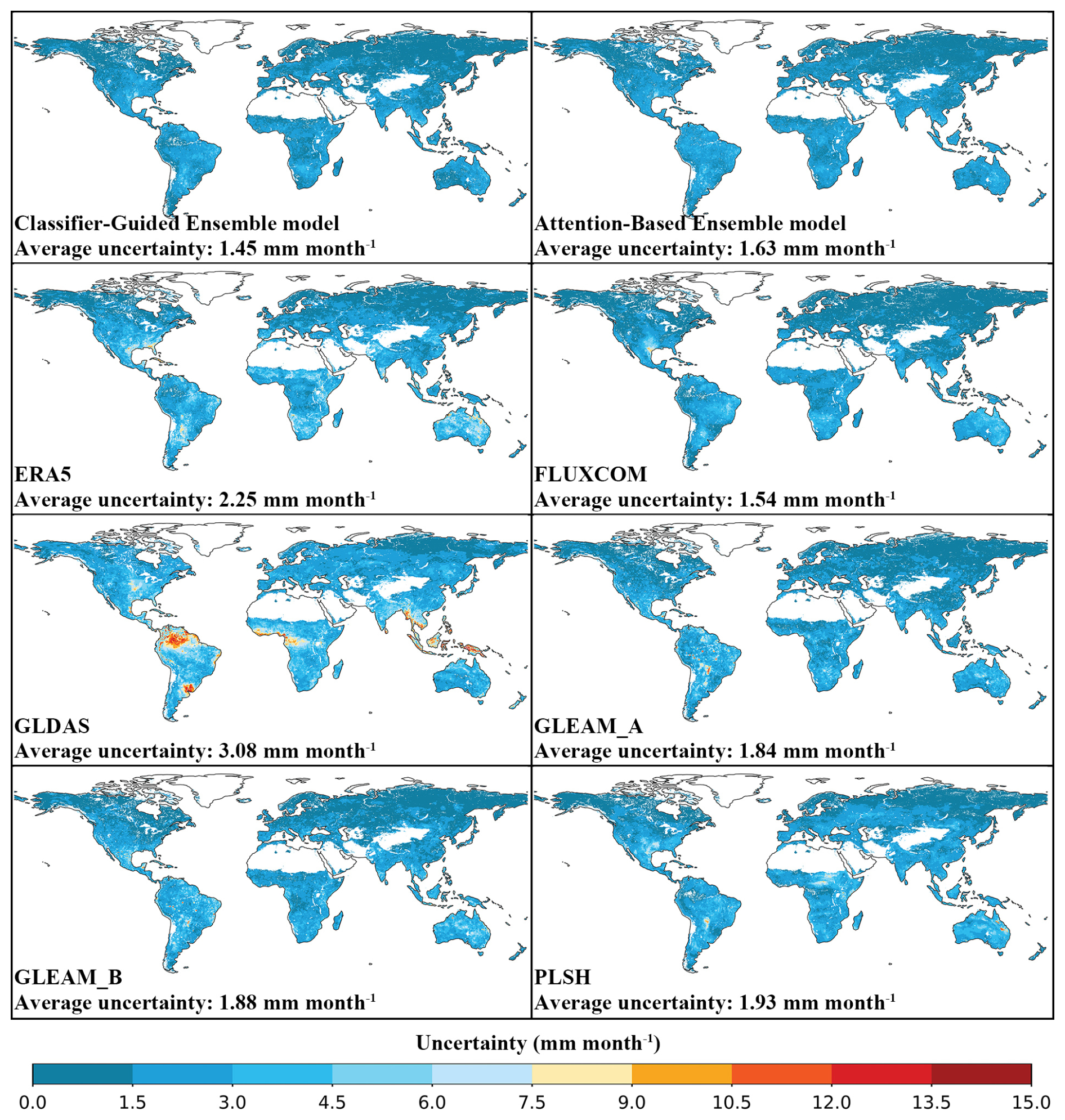
Figure 10 Average monthly uncertainty from 2005–2013 for Classifier-Guided Ensemble model, Attention-Based Ensemble model and other ET products.

Compared to Attention-Based Ensemble model, our model shows lower uncertainty in high ET regions near the equator and shows lower uncertainty compared to FLUXCOM in the southern North America and Australia. These results confirm preceding analysis that our Classifier-Guided Ensemble model consistently perform well at global scale, showcasing the potential of our ensemble method to enhance the generalizability.

5 Discussion

In this work, by developing a novel ML Classifier-Guided Ensemble ET model, we provide a simple but effective way to integrate different base models (process-based algorithm, ML-based ET model, and hybrid model) to estimate ET or similar variables lacking reliable global observations. Through the introduction of ML classifier, Classifier-Guided Ensemble model can utilize the distinct advantages of the three base models with better performance at multiple spatial scales. Compared with individual base models and Attention-Based Ensemble model, Classifier-Guided Ensemble model fit ET observations better, especially in extreme samples and under different sites and vegetation cover conditions, demonstrating improved generalizability and avoiding the underestimation of high values compared to traditional ensemble models. At catchment scale, ET estimates from Classifier-Guided Ensemble model show a greater agreement with catchment ET calculated from water balance, with performance comparable to other widely used ET products (ERA5, FLUXCOM, GLDAS, GLEAM_A, GLEAM_B, and PLSH). At global scale, the evaluation of multi-year average ET estimates and uncertainty analysis indicate that Classifier-Guided Ensemble model can provide a reasonable and stable global ET estimate. The main advantage of Classifier-Guided Ensemble model is the improved generalizability, which is primarily attributed to the introduction of ML classifier due to the ML Classifier's capacity to include a broader range of training data and to select the appropriate model at each pixel, especially for process-based algorithm.

5.1 Evaluation of the Effectiveness of ML classifier

As the additionally incorporated ML classifier is the core of the proposed ensemble framework, we further validated its effectiveness at both site and global scales. Figure 11a shows that in “process-based algorithm-dominated” type derived from in situ observations, our Classifier-Guided Ensemble model achieves better results than other models, with a KGE of 0.94, R² of 0.94, MAE of 5.07 mm per month, RMSE of 8.71 mm per month. As demonstrated by the results in Sect. 4.1.1, the process-based algorithm has a poor accuracy of ET estimation at site scale, with a KGE of 0.65, so ensemble model based on in situ observations cannot take good advantage of the process-based algorithm. In Attention-Based Ensemble model, the process-based algorithm contributes much less than the other two models, so neither ML model nor Attention-Based Ensemble model can outperform our Classifier-Guided Ensemble model when the ET estimated by process-based algorithm is the closest to the observed ET.

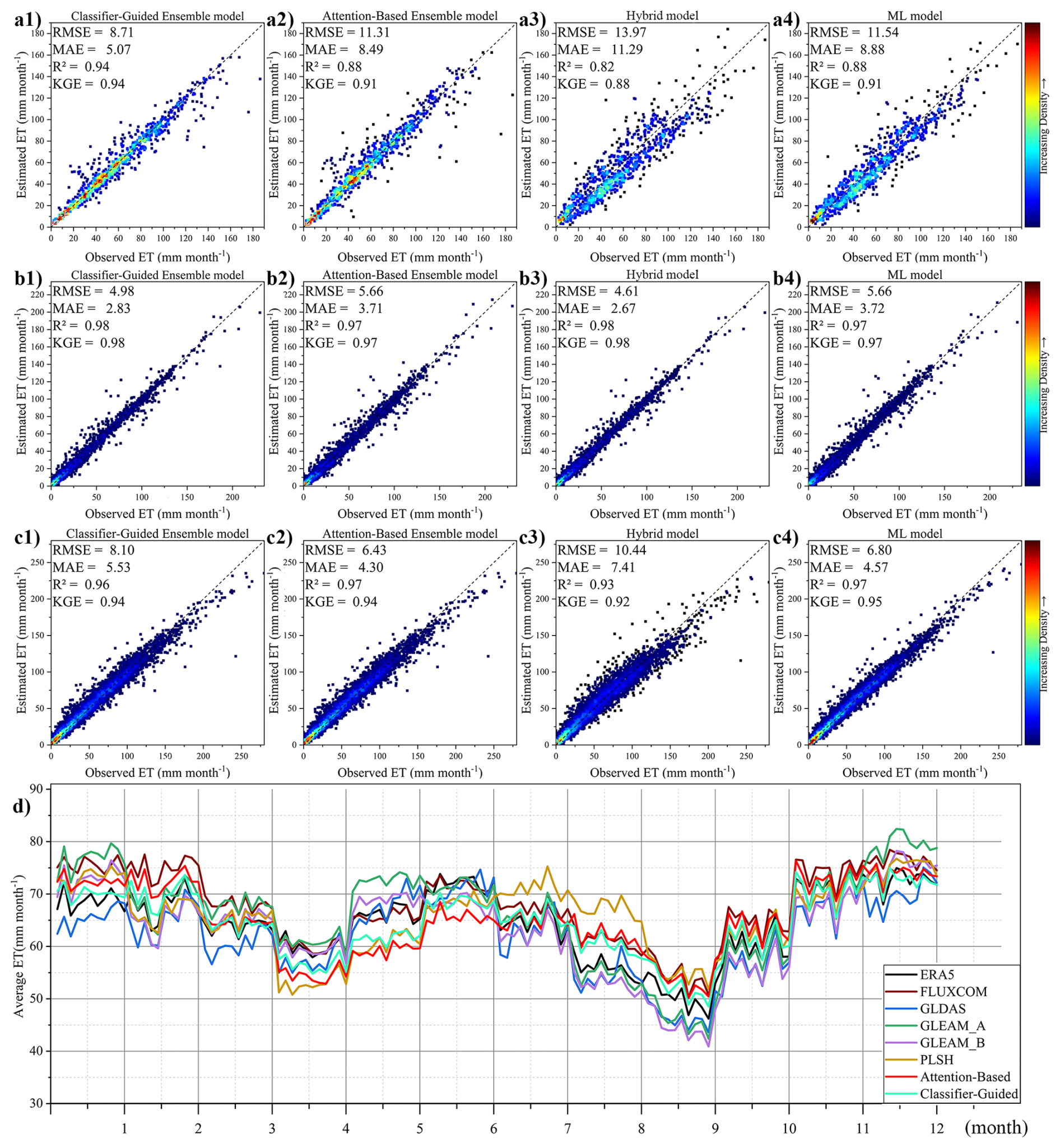
Figure 11 The comparison of model performance among (1) Ensemble model, (2) Attention-Based Ensemble model, (3) Hybrid model and (4) ML model under (a) “process-based algorithm-dominated” type, (b) “Hybrid model-dominated” type, (c) “ML model-dominated” type based on in situ observations. (d) The comparison of global average monthly land evapotranspiration from 2005–2013 under “process-based algorithm-dominated” type.

We also analyzed the case of two other types: “hybrid model-dominated” and “ML model-dominated” derived from in situ observations. In “hybrid model-dominated” type (Fig. 11b), the hybrid model performs the best as expected, with a KGE of 0.98, R² of 0.98, MAE of 2.66 mm per month, RMSE of 4.61 mm per month. Classifier-Guided Ensemble model also performs better in this case compared to Attention-Based Ensemble models, with a KGE of 0.98, R² of 0.98, MAE of 2.83 mm per month, RMSE of 4.92 mm month⁻¹. The Attention-Based Ensemble model pays more “attention” to the ML model which has higher accuracy at site scale, so in “hybrid model-dominated” type, its results are closer to the ML model, while our model can use hybrid model in most points based on the results of the ML classifier, leading to better results for our models. However, in “ML model-dominated” type (Fig. 11c), Attention-Based Ensemble model performs better than Classifier-Guided Ensemble model, with a higher R² of 0.97, lower RMSE of 6.43 mm per month and MAE of 4.30 mm per month. Classifier-Guided Ensemble model cannot perform as well as the ML model because the accuracy of ML classifier is not 100 %, while the Attention-Based Ensemble model gets better performance by combining the results of the three models.

Therefore, although our model performs well in estimating ET at various scales, there are still some limitations. The core of our model is to select the potential optimal model as “dominant model” for each pixel as determined by the ML classifier, so in regions where a single model already achieves the best results, Classifier-Guided Ensemble model does not improve performance. In this case, other ensemble model, such as Attention-Based Ensemble model, performs better, as they can improve performance by integrating multiple models.

At global scale, we also conducted additional analysis and validation of the results of the ML classifier within our model. Since ML model and Hybrid model perform well at global scale, while process-based algorithm has lower overall accuracy, we focused on whether the ML classifier can identify pixels where the process-based algorithm performs well and use it to improve the estimation robustness in these areas. Figure 11d shows the line chart of the monthly mean ET series for all datasets at the points corresponding to “process-based algorithm-dominated” type derived from the ML classifier. It is found that the Attention-Based model yields the lowest ET estimation among all datasets around May and FLUXCOM overestimates ET around February, September, October and November, while our Classifier-Guided Ensemble model shows improvements in these cases. In comparison to the Attention-Based Ensemble model's performance (R² with the various products as follows, ERA5: 0.60, FLUXCOM: 0.71, GLDAS: 0.29, GLEAM_A: 0.54, GLEAM_B: 0.51, and PLSH: 0.73), our model's results are closer to these widely used ET products (R² with the various products as follows, ERA5: 0.85, FLUXCOM: 0.72, GLDAS: 0.60, GLEAM_A: 0.67, GLEAM_B: 0.71, and PLSH: 0.84). This also demonstrates that using the process-based algorithm instead of ML models in these regions has led to an improvement in the reliability of the ET estimation. Overall, the introduction of the ML classifier did improve the performance of our model at both site and global scale.

5.2 Interpretability of machine learning used in Classifier-Guided Ensemble model

For machine learning-based models, improvement of the model performance is important, but the interpretability of the model is equally crucial. Especially for our model, the explanation of ML classifier can give us more insight into how it selects the “dominant model”, and under which meteorological conditions a particular model is preferred to be selected at both global and site scales, providing valuable support for future research. Interpretable machine learning models are gaining increasing attention, and various methods, such as LIME and SHAP, have been widely used to explain various machine learning models (e.g. Chakraborty et al., 2021; Chu et al., 2024; Eskandari et al., 2024). In this study, we used SHAP values to analyze the interpretability of the ML classifier within Classifier-Guided Ensemble model and we used both site-scale and global-scale data to calculate SHAP values.

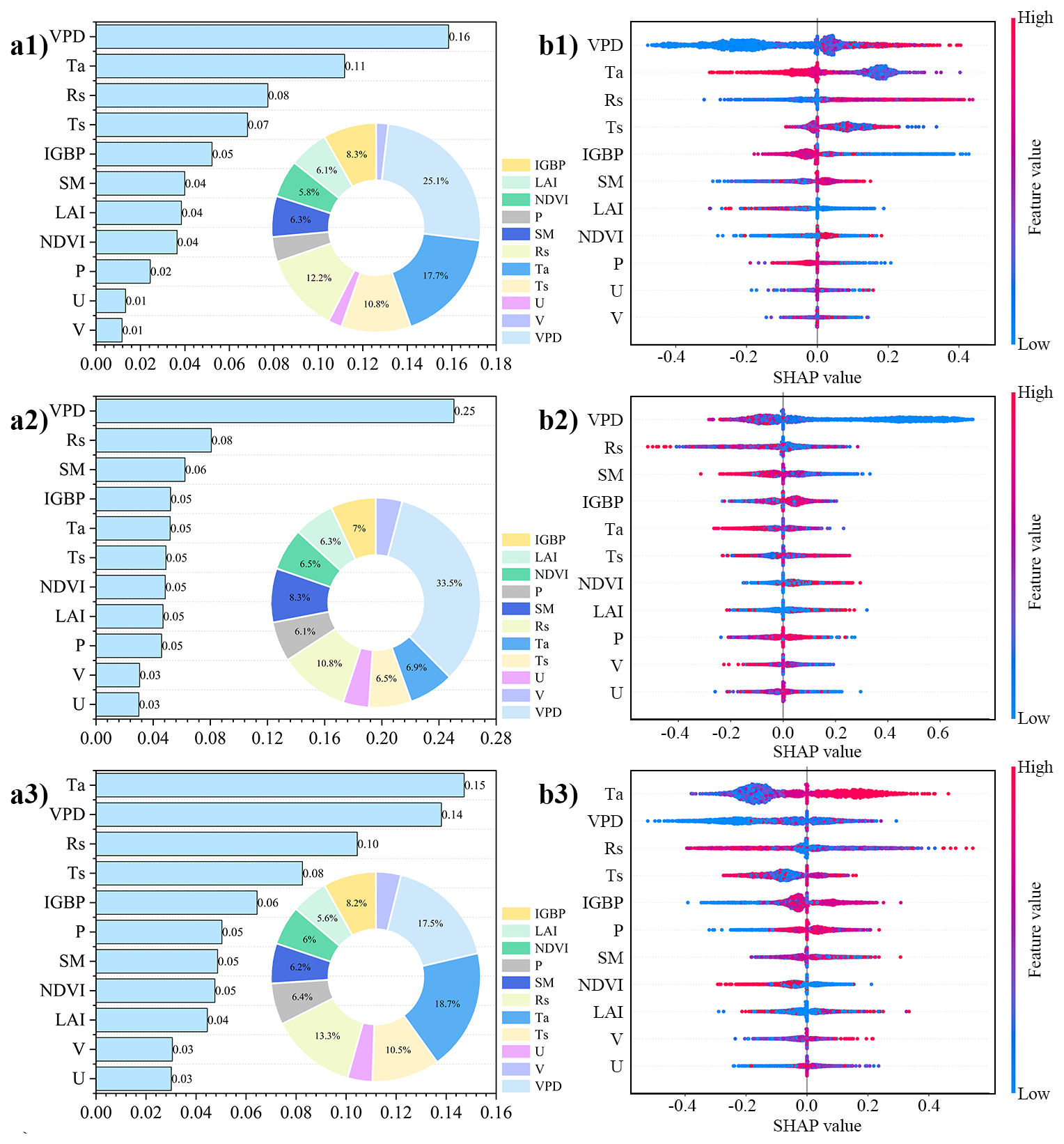
Figure 12 (a) The bar plot and (b) summary plot of the SHAP values for (1) “process-based algorithm-dominated” type, (2) “Hybrid model-dominated” type and (3) “ML model-dominated” type. The bar plot exhibits the mean absolute SHAP values for each covariate and the summary plot exhibits the distribution of SHAP values.

The contribution of different covariates to the results varies across the different classes (Fig. 12a). As Fig. 13a shows, the covariates VPD, T_a, and R_s have a higher contribution, while NDVI, LAI, P, U, and V have a lower contribution. For “process-based algorithm-dominated” type, the contribution of VPD accounts for 25.09 %, followed by T_a (17.68 %), R_s (12.22 %), T_s (10.78 %), IGBP (8.25 %), SM (6.31 %), LAI (6.08 %), NDVI (5.77 %), P (3.86 %), U (2.10 %), V (1.85 %). For “ML model-dominated” type, the distribution of SHAP values shows some similarity to “process-based algorithm-dominated” type (Fig. 13b), with T_a having the highest contribution (18.67 %) and VPD the second highest (17.52 %). Previous studies have demonstrated that variables VPD, T_a, and R_s make significant contributions to the estimation of ET, whether using machine learning methods or the process-based algorithm (Mu et al., 2011; Shang et al., 2023). The similarity in the contribution distribution of ML model and process-based algorithm may be attributed to the fact that they directly estimate ET, while differences may result from their different algorithms.

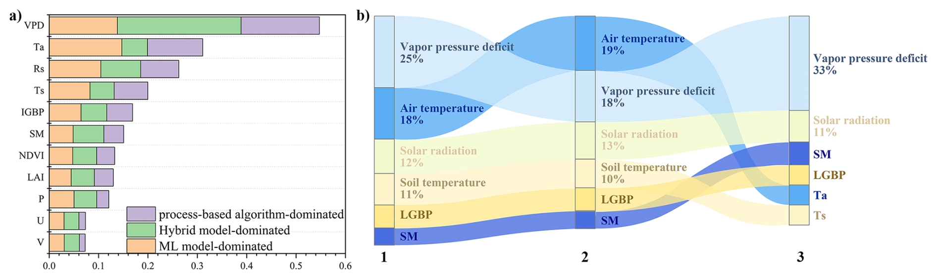
Figure 13 (a) The bar plot of the mean absolute SHAP values for three types and (b) the changes in variable contributions across (1) “process-based algorithm-dominated” type, (2) “ML model-dominated” type, (3) “Hybrid model-dominated” type.

For “Hybrid model-dominated” type, it is still VPD that dominates the feature contribution, with its proportion rising to 33.39 %. The distribution of covariates under “Hybrid model-dominated” type is somewhat distinct from “process-based algorithm-dominated” type and “ML model-dominated” type, with a higher contribution from SM and a slightly reduced contribution from T_a (Fig. 13b). Machine learning was used in the hybrid model for the estimation of r_s, and it was strongly correlated with water content (VPD, SM), and temperature (T_a) (Gan et al., 2018; Leuning et al., 2008; Mallick et al., 2015). In the hybrid model ML-GS developed by Shang et al. (2023), the distribution of SHAP values for their input variables is similar to that in our “Hybrid model-dominated” type. Therefore, it can be seen that the variables with a higher contribution when selecting the `dominant model' in the ML classifier have a certain correlation with those having a higher contribution when estimating ET.

The Fig. 12b shows the summary plot, where the horizontal axis represents the SHAP values, indicating the contribution of each covariate and color represents the magnitude of the variable values, with redder colors indicating larger variable values. The summary plot illustrates that, in certain conditions, a specific base model may have higher SHAP values, indicating its greater likelihood of being selected. For instance, under high VPD, low T_a and high R_s conditions, process-based algorithm is more likely to be selected. Also, there is a tendency to select Hybrid model under conditions of low VPD and low SM, while the ML model tends to be selected under high T_a conditions. The results in the summary plot show some correlation to the extreme samples analysis (Sect. 4.1.3) that for the 0th–1st percentiles of the VPD and SM, hybrid model outperforms ML model, making hybrid model the preferred choice. Despite these clear conditions, model selection remains unclear in some cases, particularly for ML model and Hybrid model, possibly due to their inter-correlation as both of them are based on ML method.

In summary, the interpretability analysis provides insights into the covariates with the high contribution to model selection, as well as scenarios where the three base models are more likely to be selected. However, the model selection for some cases such as high VPD, low radiation, etc. is not fully determined and further research is needed to explore the deeper mechanisms of model selection.

5.3 Uncertainties of Classifier-Guided Ensemble model

Despite better performance than other models in estimating ET at multiple spatial scales, there are still uncertainties in our model. First, the inclusion of a ML classifier in our ensemble model may introduce uncertainties. Although we used multiple global ET products as references when adding global-scale training data, these are not as reliable as ET observations, so we are still unsure of the accuracy of classification. Moreover, the classification results of machine learning model are not completely accurate, leading to the fact that the ML classifier does not guarantee optimal model selection. To minimize the impact of this issue, we have chosen models that have been shown to be excellent for global ET estimation in previous studies, so even if the ML classifier does not accurately choose the optimal model as “dominant model” at some pixels, the results of the other models will not differ significantly.

Second, the base models selected may introduce uncertainties. We chose to integrate ML-based ET models, process-based algorithms, and hybrid models. Although process-based algorithms have been widely used for ET estimation, there is still no widely recognized optimal method for the parameterization of some ET processes (Jiménez et al., 2018; Mu et al., 2011). While ML-based ET models perform well in regions with sufficient data, they tend to have poor generalizability in regions with limited data and may suffer from local optima or overfitting problems (Koppa et al., 2022; Yuan et al., 2020). For hybrid model, there are also uncertainties in the synergy between physical laws and machine learning (Shang et al., 2023).

Lastly, our model contains many input variables that incorporate multiple data sources including: satellite data, reanalysis data, and in situ observations, which may introduce uncertainty. At site scale, water flux observations obtained by the eddy covariance method have inherent random errors from the measuring instruments (Mizoguchi et al., 2009). According to the previous study, the biases between the reanalysis data and the satellite meteorological data (Rienecker et al., 2011) and the inconsistency between in situ observations and global-scale data also introduces uncertainty (Cao et al., 2021). We have made efforts to reduce uncertainties caused by data inconsistencies by replacing in situ covariate observations with the corresponding data from global-scale datasets at the same coordinates, but the uncertainties remain unavoidable.

5.4 Future perspectives

Despite the uncertainties and limitations, our model offers a new perspective on integrating multiple models and utilizing the complementarity between ML models and physical models, and there remains potential for further improvement. First, various alternatives still exist for the selection of base models. For example, there are many other ML models that can be chose and have their own advantages, such as some deep learning models (LSTM, CNN, etc.). These deep learning models or their improved forms have been shown to effectively estimate ET in previous studies (Guo et al., 2024; Karbasi et al., 2022; de Oliveira e Lucas et al., 2020). There are also some ET estimation methods based on other frameworks without using the three base models we chose, such as a Bayesian-driven ensemble learning method (Ochege et al., 2024). Better results might be obtained by choosing different models or by integrating more models, which could be a potential direction for future research.

Second, more rigorous and reasonable methods are needed for model integration. One of the advantages of the proposed framework is that we can add global data as training data even when there are no global-scale observations, which offers a novel approach to improving the generalizability of model, but how to identify the “dominant model” from additional data remains a problem. If there is a more rigorous and reasonable method to optimize the model selection, it can not only improve the reliability of the final ET estimation, but also contribute to the study of the regions where each base model demonstrates its advantages. Additionally, after the ML classifier has selected the “dominant model” at each pixel, if we discard the simple use of the selected model and adopt more advanced methods for model integration, the results of Classifier-Guided Ensemble model may be further improved. We have tried optimizing the results under three different classes using both genetic algorithms and machine learning models, but the results were not as good as expected. Since these methods are still limited by in situ observations, they do not perform as well as using the original models directly when upscaled to a global scale. It is still worth exploring how to better utilize these models.

Finally, more effective integration of machine learning and physical models has the potential to further improve ET estimation. Since physical models have higher interpretability and extrapolation capabilities, while machine learning can utilize data more effectively, how to better integrate the complementary advantages of them is a topic worthy of in-depth investigation. Moreover, ML models, especially deep learning models, are data-driven, but the available data cannot provide sufficient information for ML models to achieve better results. Leveraging physical models to extract more meaningful information from limited data is a viable way to enhance model performance.

6 Conclusions

The poor generalizability is a common limitation across ML-based global ET models due to the sparse distribution of in situ observations. In this study, we developed a novel ensemble framework for combining the distinct advantages of process-based algorithms (extrapolation performance in data-sparse regions), ML-based ET models (data adaptability in data-dense regions), and hybrid models (overall performance) by introducing an additional ML classifier. Taking advantage of the ML classifier's capacity for automatic model selection, we are able to improve the generalizability of ML-based ET models by employing physically-founded process-based algorithm and hybrid model at appropriate pixel and avoid the typical underestimation of high values by ensemble methods.

The evaluation results across site and catchment scales indicate that our Classifier-Guided Ensemble model is overall more accurate than the individual base models, Attention-Based Ensemble model and other widely used global terrestrial ET products (ERA5, FLUXCOM, GLDAS, GLEAM_A, GLEAM_B, and PLSH) with lower RMSE and MAE and higher R² and KGE, especially in extreme samples where existing ML models perform poorly. At global scale, our model also exhibits higher stability, as well as greater consistency with these global ET products in both spatial patterns and latitude-averaged values.

In addition, the analysis of ML classifier's effectiveness demonstrates that the ML classifier can reasonably select the base models used at both global and site scales, highlighting the potential to further enhance the model's generalizability. Moreover, by further analyzing the SHAP values of different input covariates when the ML classifier select the “dominant model”, we gained a simple understanding of the mechanisms behind the selection of “dominant model” that just as VPD, T_a, and R_s are critical for ET estimation, these variables also play a crucial role in model selection and identified some specific scenarios in which each model is most suitable. However, we chose to introduce global-scale training data to enhance the generalizability of the ML classifier, which has indeed led to improvements in ET estimation, but since these data were not obtained from ET observations, this may introduce uncertainties. Therefore, while our framework demonstrates significant potential to advance global ET estimation, further in-depth analysis and investigation are required, especially for the introduction of the ML classifier.

Appendix A: Supplementary tables

Table A1 Information for the 129 EC Flux Tower Sites, including the Site Name, Latitude (Lat), Longitude (Lon), International Geosphere-Biosphere Programme Land Cover Types (IGBP).

Table A2 Information for the 38 Selected Catchments.

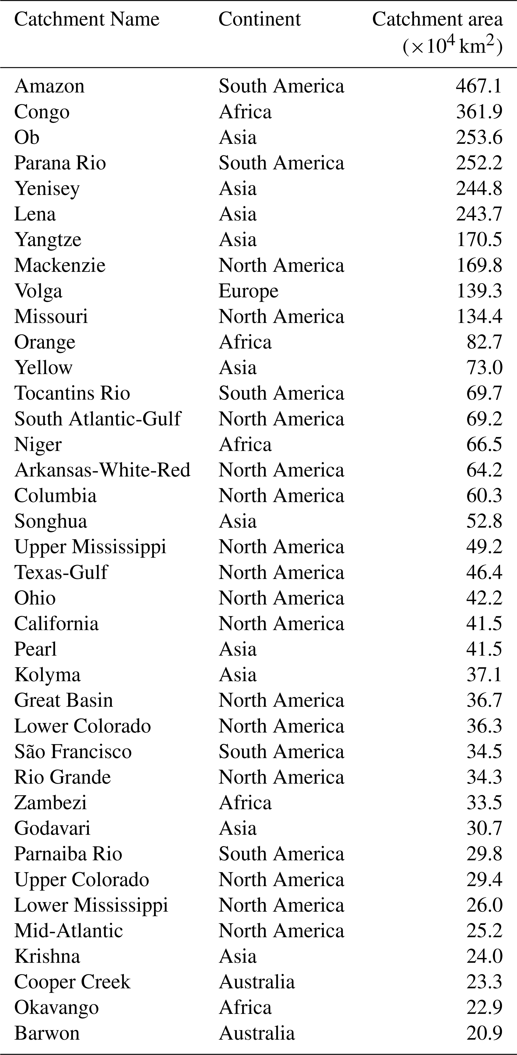
Table A3 Information for the 30 Selected EC Flux Tower Sites in Independent Validation.

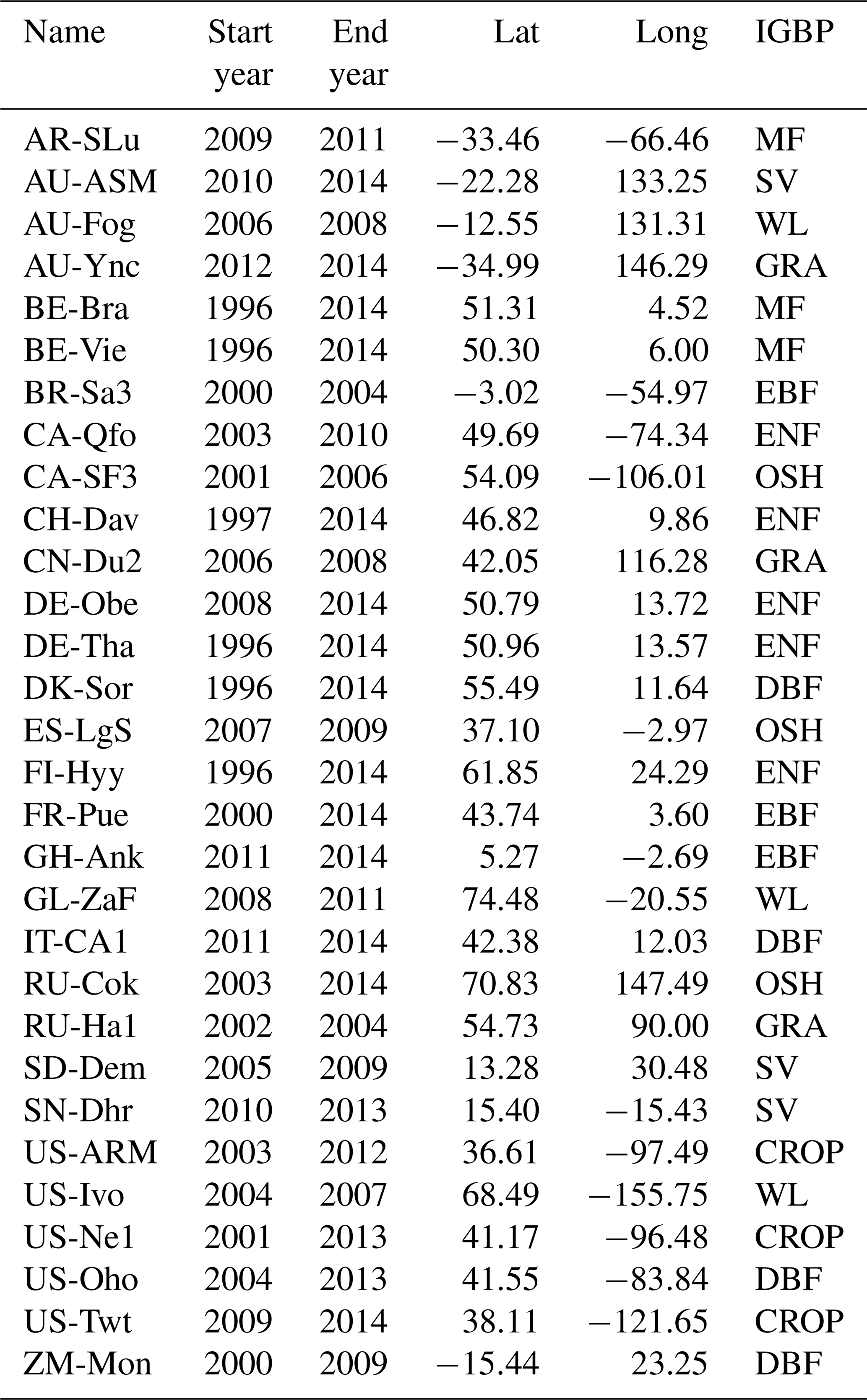
Table A4 Performance of Different ET Models in Independent Validation.