A simplified model to investigate the hydrological regimes of temporary wetlands: the case study of Doñana marshland (Spain)

Natural and pristine ecosystems, such as wetlands, are being either directly or indirectly threatened by a multiplicity of drivers, which include anthropogenic activities and the impacts they have on the use of natural resources. Strategies oriented to a sustainable management of natural resources (in particular, water) are therefore urgently needed, considering also the increasing effects of climate change. Despite their ecological importance, wetlands remain underrepresented in hydrological modelling studies, especially regarding their specific water needs under changing environmental conditions and different scenarios. This study aims to estimate the water requirements of a temporary wetland through a simple hydrological balance model, ultimately facilitating the identification of strategies for its long-term sustainable management. The pilot case study is the Doñana National Park, SW Spain, one of the case studies of the European project LENSES (PRIMA Call 2020). The model (“WetMAT”) is calibrated and validated using historical time series of key hydrological variables (Maximum Flooded Area and Hydroperiod) taken from the literature, to describe the hydrological processes in the wetland. The model is then used for a scenario analysis focused on the assessment of climate change impacts on the state of the wetland and for assessing the ecological water demand of the wetland in a dynamic way, helping to quantify the water needs of such a fragile ecosystem. The results highlight the urgency and importance of developing tools that can help integrating environmental needs into water resources planning and management.

1 Introduction

In the current era human activities increasingly seek and depend on natural resources, often exploiting them beyond their regenerative capacity (Corlett, 2015). These resources have supported major societal transformations, including urban expansion and rapid population growth, but are now strictly limited and several approaches are being considered to support their integrated and sustainable management (Wu et al., 2023). The uncertainty related to climate change adds complexity and poses increasing risks to the availability and use of resources (Iglesias et al., 2006; Garrote, 2017). Within this context, natural areas and their ecosystems pay the consequences of such changes without being able to adapt (Schlaepfer and Lawler, 2023). Understanding how to cope with these changes by finding adaptation strategies is therefore increasingly needed (Falkenmark et al., 2019).

Wetlands (which are broadly defined by the Ramsar Convention of 1971 as transitional zones between aquatic and terrestrial ecosystems) are critical environments. They include a wide range of environments, both permanent and temporary, natural or artificial systems, which range from marshes to peatlands (Finlayson et al., 1995). Permanent wetlands have water throughout the year, supporting a stable aquatic ecosystem, while temporary wetlands are subject to seasonal or intermittent flooding, and water is present only during specific periods, often leading to unique ecological dynamics (Boix et al., 2020). The relevance of wetlands relates to the multiplicity of ecosystem services (ESs) they provide, such as climate regulation, flood protection, carbon sequestration, support for biodiversity, as well as socio-economic and cultural benefits that contribute to human well-being (Bhowmik, 2022). Besides providing a multiplicity of ESs, wetlands are also excellent markers for recording the effects of climate change (Vanderhoof et al., 2018) as very often the adaptation strategies of these ecosystems are slower than the changes they are impacted by Schröter et al. (2019). There is evidence of the climate and anthropogenic impacts at every latitude (Khelifa et al., 2022) and, in particular for temporary wetlands, of an increasing tendency to disappear or deteriorate (Havril et al., 2018). Wetland hydrology relies on a variety of approaches (Lee et al., 2020). Surface and groundwater hydrological modelling techniques are commonly employed, often limited by the frequent absence of sufficient gauging stations within wetlands, which restricts the accuracy of conventional hydrological models (Chomba et al., 2021). Remote sensing techniques (such as drones and satellite imagery) have also become increasingly widespread (Adam et al., 2010; He et al., 2022), as they enable the acquisition of large-scale, real-time data, effectively overcoming the limits associated with the extensive and variable nature of wetland ecosystems (Wu, 2017; Zhao et al., 2025). However, there are limitations, such as the high costs of high-resolution data acquisition, difficulties in data interpretation due to vegetation or environmental conditions and the scarcity of ground validation data in remote areas (Abdelmajeed and Juszczak, 2024). Independent on the approach adopted, the ecological processes related to water are often overlooked, which results in an insufficient evaluation of ESs (Xu et al., 2018), and ultimately in an incomplete understanding of wetland dynamics (Xu et al., 2020). Another gap lies in the limited representation of the temporal dynamics of these environments (Zhang et al., 2016), which is particularly evident when assessing climate change impacts (Liu and Kumar, 2016).

To address these gaps, it is essential to use integrated and dynamic tools for wetland analysis (Manzoni et al., 2020) that can help include multiple dimensions and dynamics (Ding et al., 2024), while making explicit the active role of ecosystems, that should not be merely considered a passive backdrop (Hülsmann et al., 2019). Identifying environmental water requirements is inherently complex, as these needs are not explicitly stated or easily quantifiable (Cosgrove and Loucks, 2015), and an additional effort is required in temporary wetlands, whose hydrological processes are particularly complex (Angeler, 2021).

This study details a simple hydrological balance model, WetMAT (Wetland MAnagement Tool), which has been developed to simulate the flooding and drainage dynamics of temporary wetlands. It has been developed and tested in the Doñana National Park (Spain), but its simple conceptual structure is intended to facilitate its application to other wetland systems, where different variables (salinity, water level, extension of flooded areas) can be used for calibration and validation processes according to the specific characteristics and data availability of each case study. Differently from available models, which would require a lot of input data (e.g., soil characteristic, soil-water interactions, topography, vegetation), WetMAT proposes a simplified approach based on lumped modelling. The structural and computational simplicity, combined with its daily temporal resolution and strong correlation with meteorological data, allows for accounting for climate change and implementing scenario analyses for evaluating mitigation strategies: the Inundation Persistence Index (IPI) is introduced for this purpose, defined here as a synthetic and physically interpretable metric of marshland inundation dynamics. By integrating information on spatial magnitude of inundations and their temporal persistence, IPI can support inter-annual comparisons and provides a concise basis for scenario-based evaluations. More specifically, in the present work, we aim to address the following research questions: (i) Can a simplified hydrological model effectively reproduce the flooding and drainage dynamics of a temporary wetland? (ii) Can WetMAT support hydro-ecological assessment? (iii) Can it produce actionable information to support decision-makers?

The paper is structured as follows. The Sect. 2 provides a detailed description of the case study and its main challenges. It also includes an in-depth presentation of the WetMAT model, focusing on its operating processes and the key governing equations. Section 3 summarizes the main Results, with a focus on the sensitivity analysis, and on the calibration and validation processes. Climate change scenarios are also detailed. Section 4 provides a thorough discussion on the results obtained, highlighting limitations, strengths and replicability of the proposed model. Finally, future developments of WetMAT are presented in the Sect. 5.

2 Material and Methods

2.1 The case study

The Doñana region (37° N, 6° W) is an area overlooking the Atlantic Ocean bordered by the Guadalquivir River estuary to the East and the Tinto River estuary to the West (see Fig. 1). Located in the SW of Spain, Doñana hosts the largest wetland in the Country and one of the largest in Europe, with significant ecological importance, particularly as a migratory stop for birds, hosting 75 % of European bird species (Fernandez-Delgado, 1997). From the demographic point of view, the Doñana region collect about 200 000 inhabitants, and the main economic activities of the area concern tourism and agriculture, particularly berries (Palomo et al., 2011).

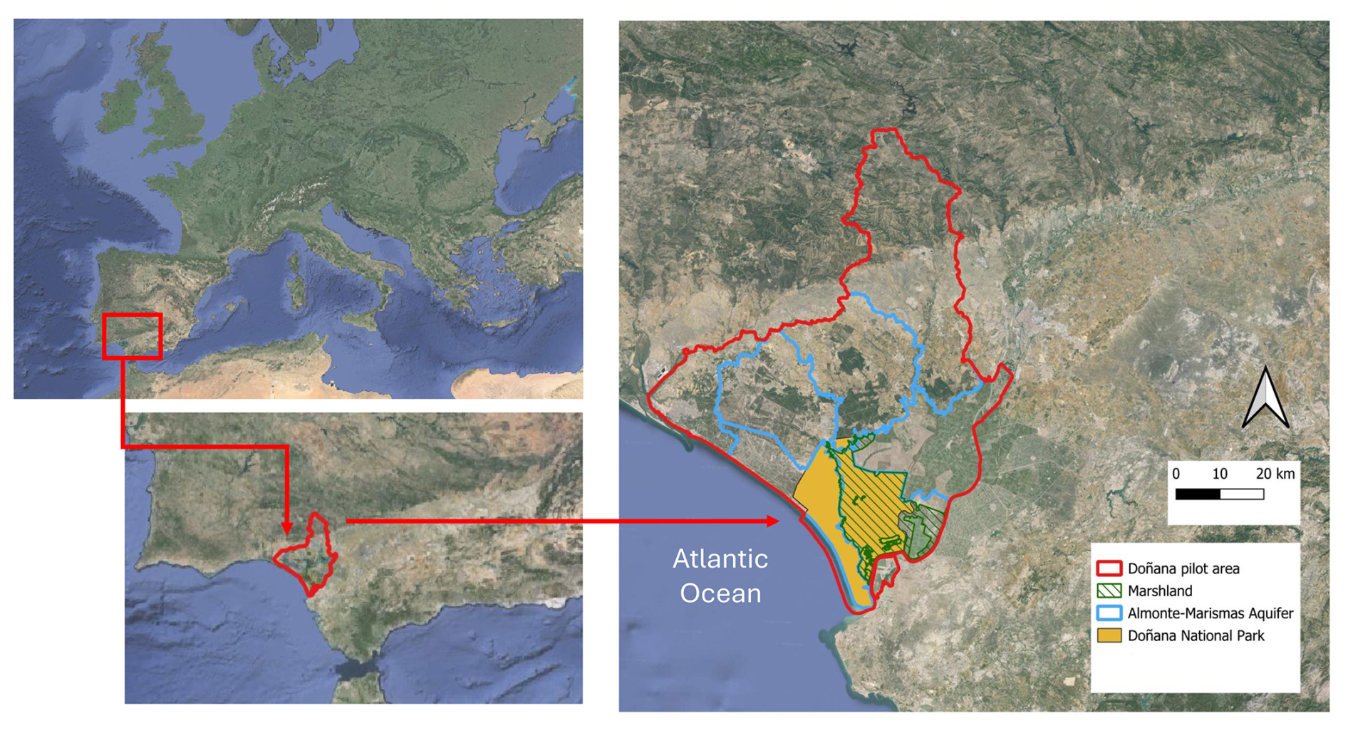
Figure 1 Overview of the study area and its major aquifers (elaboration from © Google Earth 2024).

Doñana has a sub-humid Mediterranean climate, with an average annual rainfall around 540 mm although precipitation varies significantly due to Atlantic influence (Serrano, 2016). Climatic projections show also a potential gradual increase in temperatures over time.

The natural context of Doñana includes marshes, sand dunes with temporary ponds, coastal systems and estuary (Zorrilla-Miras et al., 2014). The marshland, which is the focus of the present work, consists of a flat area with slight depressions (“lucios”) and rises (“vetas”), which are not flooded during peak flooding events, and received originally flow from several streams such as the Guadiamar, El Partido and La Rocina (Serrano et al., 2006). At the beginning of 20th century, the natural marshland covered an area of 1500 km², but it has been reduced by about 80 % over time, now spanning around 300 km² largely due to agricultural development occurred over the course of the last century (Leiva-Piedra et al., 2024).

The underground hydrology is also complex, characterized by a confined aquifer beneath the marshland and an unconfined, rainfall-fed aquifer in the coastal zone (Suso and Llamas, 1993). These aquifers, according to different monitoring systems, are in poor quantitative and/or qualitative status (CHG, 2022).

However, Doñana's marshland is isolated from direct groundwater exchange by a clay layer (Naranjo-Fernández et al., 2018).

Several forms of protection have been implemented in the Doñana area since 1969, with the establishment of Doñana National Park. It was recognized as International Biosphere Reserve in 1980, officially recognized by the Ramsar Convention for wetlands in 1982 and a World Heritage Site in 1995 by UNESCO. However, in 1990, Doñana also returned to the Montreux Record of Ramsar Sites Under Treat, mainly considering the pressures from agricultural expansion, groundwater overexploitation and tourism (Serrano and Serrano, 1996; Sousa et al., 2009; Martín-López et al., 2011). In particular, the establishment of the Lower Guadalquivir Irrigation Area (in the mid-20th century), encouraged by the Spanish government, led to the regulation of the Guadiamar River, effectively isolating the marshland's primary water supply through the “Entremuros” project. Additionally, in 1998 the accidental collapse of the Aznalcollar dam forced local authorities to further isolate the wetland from the Guadiamar River to preserve it from the large volumes of toxic sludge. Nowadays, despite attempts to restore the natural waterways, the marshland is no longer fed by the river Guadiamar or its tributaries (Baena Escudero and Guerrero Amador 2006). Significant groundwater withdrawals continue to cause substantial declines in the water table, resulting in a reduction of the spring flow at the marshland's edges (ecotones) (Díaz-Paniagua and Aragonés, 2015). For all these reasons the Doñana area represents a complex environment (Gil Gil and Schmidt, 2024), with severe anthropic pressures on the natural environment, and a multiplicity of stakeholders involved in (and impacted by) its management.

2.2 The WetMAT model

2.2.1 Model description

The WetMAT (Wetland MAnagement Tool) model is a mathematical model for a dynamic analysis of wetlands, focused on the estimation of environmental water needs based on its main hydrological processes. The WetMAT model is particularly oriented to the analysis of temporary wetlands, which have a lower hydroperiod compared to permanent aquatic systems (Calhoun et al., 2017). The hydroperiod, a variable related to inundation timing, duration and frequency, plays a crucial role in shaping the ecological structure and function of wetlands by influencing the distribution of plant and animal species (Mitsch and Gosselink, 2007). From the conceptual point of view, wetland flooding directly relates to the annual course of the precipitation. So, there is typically a wet season, generally starting in October and ending in late Spring for the Northen Emisphere, and a dry season, generally from April to September, when the evapotranspiration process is predominant over precipitation (Fernandez-Carrillo et al., 2019). At the beginning of the wet season, rainfall contributes to the imbibition of the soil. Once the soil is saturated, ponding originates within the most depressed areas of wetland. During the Winter season, with the increase of frequency and intensity of rainfall, the most significant flooding occurs. As the soil is saturated and the most depressed areas filled, wetland starts to flood almost uniformly. During the Spring season, when rainfall events start reducing and temperatures rise, flooded areas reduce, and the small soil depressions start to drain out. During Summer the contribution of precipitation is completely missing while evapotranspiration reaches its annual peak: the drying process of the marshland continues involving also the soil. The whole process is cyclical, although it varies from year to year depending on the variability of rainfall.

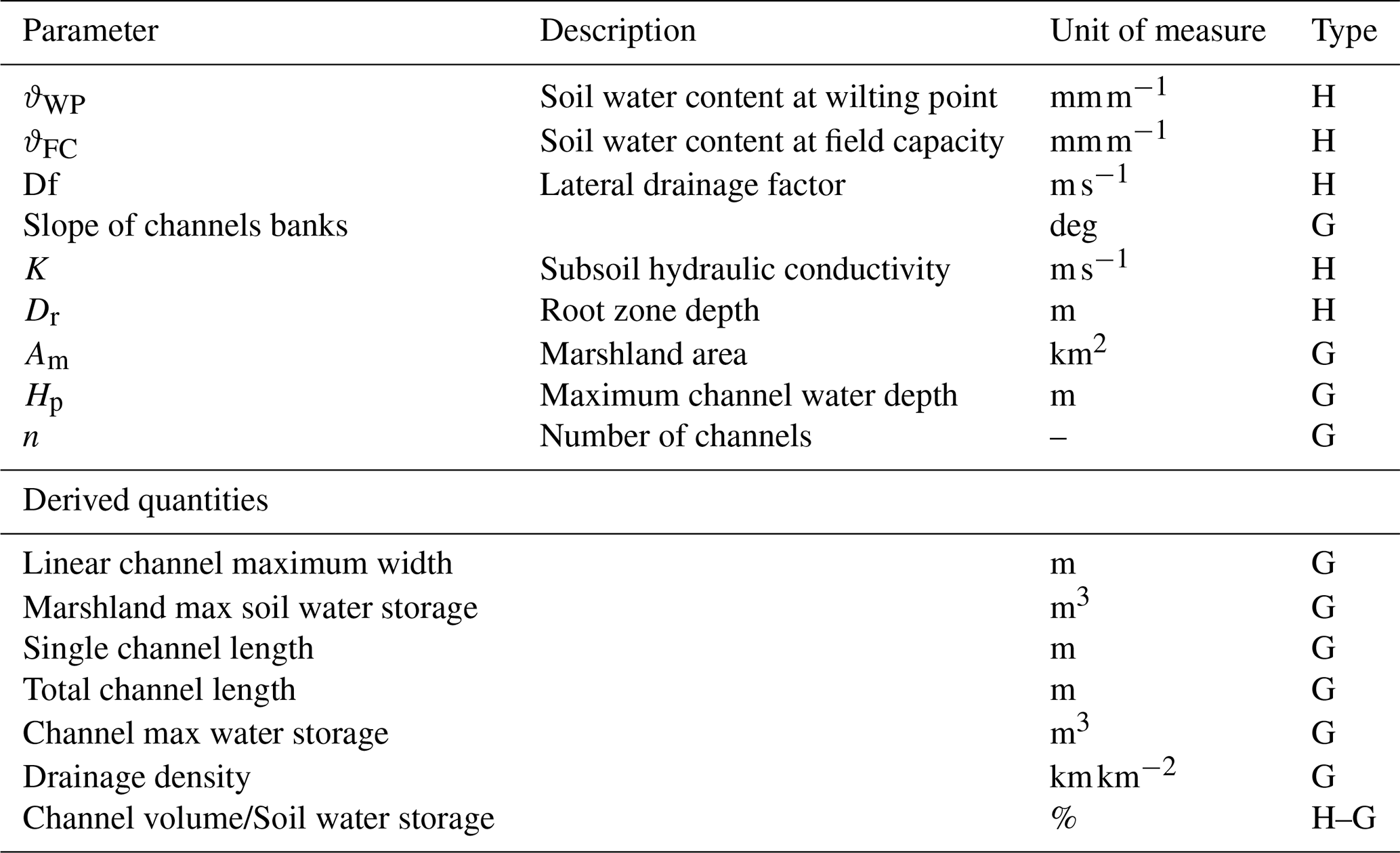
Going further into details, the WetMAT model structure relies on nine parameters, which must be defined by the analyst or taken from the case study in order to represent the system, and on a simplified system sketch. Some parameters depend on pedology and land cover of the area, i.e. the soil water content at wilting point and field capacity (ϑ_WP,ϑ_FC), the lateral drainage factor (Df), the subsoil hydraulic conductivity (K) and the root zone depth (D_r). Other parameters of the model refer to system hydrogeomorphology i.e., the slope of channels banks, the marshland area (A_m), the maximum channel water depth (H_p), the number of channels (n). Once these parameters are set, other variables are calculated. These include the linear channel maximum width, the marshland maximum soil water storage, the single channel length, the total channel length, the channel maximum water storage and the drainage density. Table 1 summarises the characteristics of the parameters and quantities described. In the “Type” column it is indicated with “H” the reference to hydraulic characteristics, and with “G” if it refers to hydrogeomorphologic ones.

Table 1 Parameters and derived quantities used by WetMAT model.

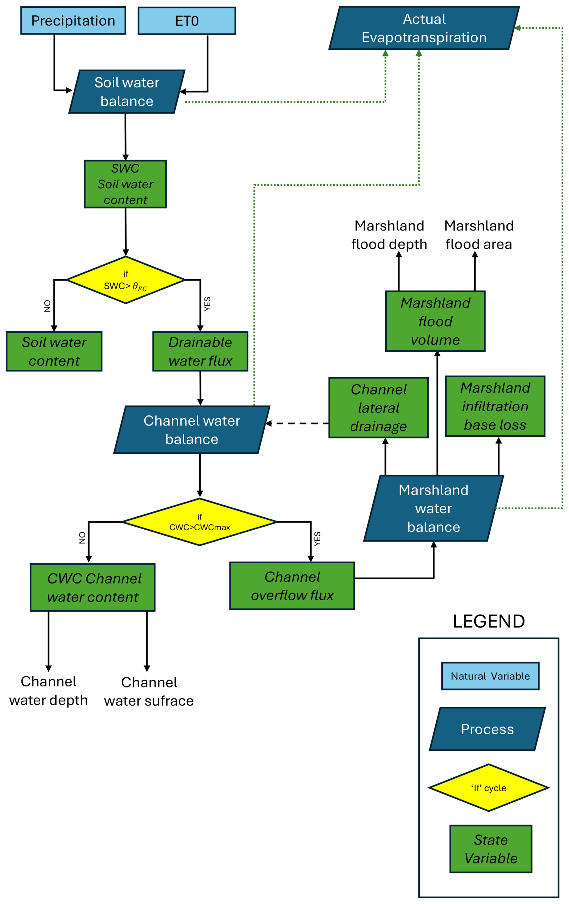
The wetland flooding and drainage process during the seasons described above is reproduced by the WetMAT model at daily scale through three different but interconnected balance processes, as shown in the flowchart of Fig. 2. First, a Soil Water Balance is performed: when the soil is saturated, a “drainable water flux” is generated, which is the input of a Channel Water Balance. When the channels are saturated as well, the excess water volume, namely a “channel overflow flux”, originates the marshland flooding. The Marshland Water Balance lastly describes the wetland flooding phenomenon and allows the computation of key variables such as the flooded area. A further process, acting on all three balances, is also represented, namely that of Actual Evapotranspiration. Additional phenomena such as lateral drainage through channels and vertical losses contribute to the marshland emptying process.

Figure 2 WetMAT model flowchart.

The following Eq. (1) is the total daily budget equation on which the WetMAT model is based. It describes the overall wetland balance in the most general form.

$$\begin{array}{}\text{(1)}& {\displaystyle \frac{\mathrm{d}{V}_{\mathrm{w}}}{\mathrm{d}t}}=P+I_{\mathrm{w}}+G_{\mathrm{w}}-O_{\mathrm{w}}-D_{\mathrm{w}}-\text{ET},\end{array}$$

In Eq. (1), $\mathrm{d}{V}_{\mathrm{w}}/\mathrm{d}t$ [m³ d⁻¹] is the volume of water that floods the marshland during each timestep. P [m³ d⁻¹] is the daily inflow from precipitation, I_w [m³ d⁻¹] is the wetland inflow from rivers and G_w [m³ d⁻¹] is the wetland inflow from groundwater. O_w represent the outflows from the wetland, i.e. a river discharge or a direct sea discharge. ET represents the daily evapotranspiration: this term aggregates evapotranspiration from vegetated surfaces, affecting the entire marshland area, and open-water evaporation from the intermittently inundated portions of the wetland, whose surface varies in time with the flooded extent. Lastly, the term D_w [m³ d⁻¹] represents the lateral drainage of the channels, which depends on the drainage density and on the main geomorphologic characteristics of the channel. The equations of the three different balances are proposed in the following to facilitate the analysis of the individual processes in detail. The Soil Water Balance is mainly based on the calculation of the soil water content SWC according to Eq. (2):

$$\begin{array}{}\text{(2)}& {\text{SWC}}_t=max({\mathit{\vartheta }}_{\text{WP}};{\mathit{\vartheta }}_{t-\mathrm{1}}+P_{t-\mathrm{1}}-{\text{ET}}_{t-\mathrm{1}}),\end{array}$$

where P is the precipitation in the previous temporal step, the actual evapotranspiration ET of the previous temporal step is calculated as a function of the potential evapotranspiration ET₀ using the Hargreaves–Samani formula (Hargreaves and Samani, 1985) and the hydraulic soil parameters according to the following Eq. (3):

$$\begin{array}{}\text{(3)}& \text{ET}={\text{ET}}_{\mathrm{0}}\left({\displaystyle \frac{\mathit{\vartheta }-{\mathit{\vartheta }}_{\text{WP}}}{{\mathit{\theta }}_{\text{FC}}-{\mathit{\theta }}_{\text{WP}}}}\right),\end{array}$$

where ϑ is the actual water content in the soil [mm m⁻¹], ϑ_WP is the wilting point capacity's soil water content and θ_FC is the field capacity's soil water content [mm m⁻¹]. In case SWC>θ_FC the soil produces a surplus, called Drainable Water Flux, which feeds the second balance of the model i.e. the Channel Water Balance. The Channel Water Balance is described by Eq. (4):

$$\begin{array}{}\text{(4)}& \begin{array}{rl}{\displaystyle }{\text{CWC}}_t=& {\displaystyle }max[\mathrm{0};{\text{CWC}}_{t-\mathrm{1}}+min({\text{DWF}}_t;{\text{CWC}}_{\text{max}}-\\ {\displaystyle }& {\displaystyle }{\text{CWC}}_{t-\mathrm{1}})-{\text{ET}}_t\times {\text{Ap}}_{t-\mathrm{1}}+P_t\times {\text{Ap}}_{t-\mathrm{1}}],\end{array}\end{array}$$

where CWC [m³], i.e. the Channel Water Content, is compared to its maximum value CWC_max [m³], depending on the geometric characteristics of the system. DWF [m³ d⁻¹] is the Drainable Water Flux, i.e. the surplus of water which cannot be absorbed by the soil in the Soil Water Balance. Ap is the Channel Water Surface in the previous time step. Unlike Soil Water Balance where soil characteristics are predominant, the Channel Water Balance mainly depend on system geomorphology. The water content in the channels of the previous temporal step and the available Drainable Water Flux are considered. In addition, Eq. (4) considers the balance of direct evapotranspiration (ET) and precipitation (P) on the channel. The Marshland Water Balance is mainly expressed through the variable Marshland Flood Volume (MFV) [m³], represented by the following Eq. (5). Again, the Marshland Water Balance is triggered by an “overflow flux” from channel overflow, responding to the condition “CWC>CWC_max”.

$$\begin{array}{}\text{(5)}& \begin{array}{rl}{\displaystyle }{\text{MFV}}_t=& {\displaystyle }max(\mathrm{0};{\text{MFV}}_{t-\mathrm{1}}+{\text{COF}}_t+{\text{MFA}}_{t-\mathrm{1}}\times P_t\\ {\displaystyle }& {\displaystyle }-{\text{MFA}}_{t-\mathrm{1}}\times {\text{ET}}_t-{\text{CLD}}_{t-\mathrm{1}}-{\text{MIL}}_{t-\mathrm{1}}),\end{array}\end{array}$$

In Eq. (5) above, COF [m³ d⁻¹] is the “Channel Overflow Flux”, the amount of water flowing from channels once they have reached the CWC_max. MFA stands for “Marshland Flooded Area” and it is expressed as a simple power-law function of MFD, following the depth–area relationships commonly adopted for shallow wetlands and low-relief basins (e.g. Hayashi and van der Kamp, 2000), and the exponent in Eq. (6) (empirical) was fixed at 0.2 for parsimony:

$$\begin{array}{}\text{(6)}& \text{MFA}=A_{\mathrm{m}}\times {\text{MFD}}^{\mathrm{0.2}},\end{array}$$

The Channel Lateral Discharge (CLD) [m³ d⁻¹] and the Marshland Infiltration Loss (MIL) [m³ d⁻¹] represent the losses in the marshland. Specifically, CLD refers to the lateral drainage of the channels, taking into account their hydrogeomorphological characteristics. MIL addresses the vertical losses from the floods, assuming a clayey soil and a very low drainage rate.

Based on the set of Equations above, the model aims to reproduce in a simplified yet consistent way the marshland flooding process. The variable MFA [km²] calculated on a daily basis, provides spatial information such as the maximum annual flooded area recorded for each hydrological year. Through the analysis of MFA is also possible to calculate how many days per year flooding of the marshland is observed (hydroperiod), so obtaining temporal information about the flooding and draining processes in the system. In particular, the mean hydroperiod is calculated in WetMAT by counting, yearly, the number of days in which the marshland is flooded and the average value for the flooded area.

2.2.2 WetMAT implementation in the Doñana marshland

The following Fig. 3 shows the WetMAT scheme for the Doñana case study as described above.

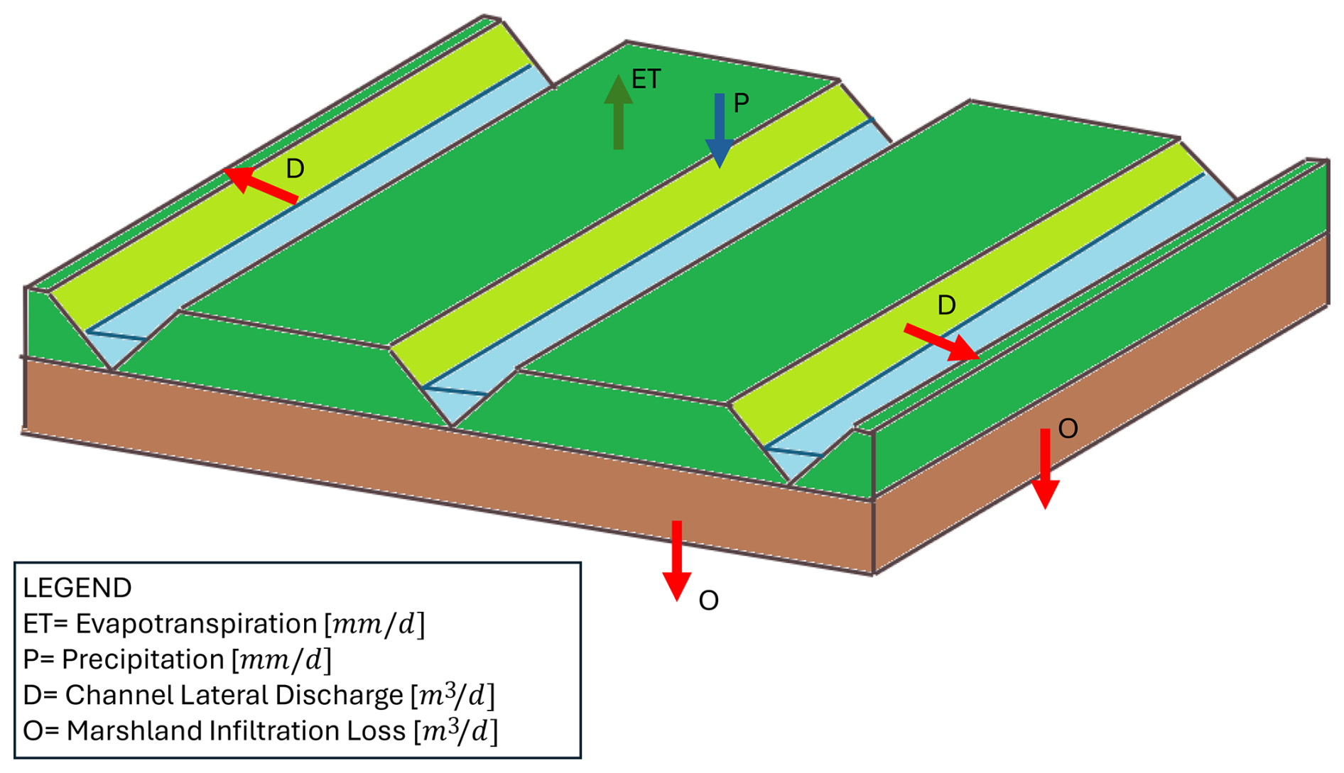
Figure 3 WetMAT model scheme for the Doñana case study, with evapotranspiration (ET) and precipitation (P) as main fluxes, small losses due to infiltration (O) and the Channel Lateral Discharge (D) affecting the marshland flooding process.

The WetMAT is used in the Doñana marshland case study based on the following assumptions.

The Doñana wetland is a flat area with small depressions, which is described in the WetMAT model as a square area and a series of identical, equidistant, triangular channels. The term I_w in Eq. (1) can be disregarded in this case study because hydraulic works carried out during the 20th century to channel the courses of Guadiamar and Guadalquivir rivers have substantially altered the wetland's hydrology so it can be considered hydraulically disconnected from its main original sources of surface-water supply (Morris et al., 2013). The term G_w in Eq. (1) is likewise negligible, leading to a further simplification of the model: over the last thirty years, piezometric levels in the aquifer have declined by up to 20 m in some points, probably due to numerous irrigation withdrawals (Green et al., 2024), resulting in the total or partial drying up of the minor watercourses that flowed into the marshland and, above all, in the reversal of the vertical hydraulic gradient in the natural discharge areas on either side of the area, i.e. ecotones. For the purpose of the present case study, a vertical leakage rate is only provided, which depends on the current flooded area and the estimated hydraulic conductivity of the subsoil. As it is mainly constituted by clay, its contribution is negligible compared to ET, the daily evapotranspiration, which constitutes the main dynamic loss component of the balance and varies over time depending on the extent of the flooded area of the marshland. The WetMAT simple balance for the Doñana case study is hence expressed by Eq. (7):

$$\begin{array}{}\text{(7)}& {\displaystyle \frac{\mathrm{d}{V}_{\mathrm{w}}}{\mathrm{d}t}}=P-O_{\mathrm{w}}-D_{\mathrm{w}}-\text{ET},\end{array}$$

2.2.3 Model parameters

Regarding Doñana marshland, Table 2 shows the ranges of values recommended in the literature and selected for each parameter.

Table 2 Parameters' ranges and default values for Doñana case study.

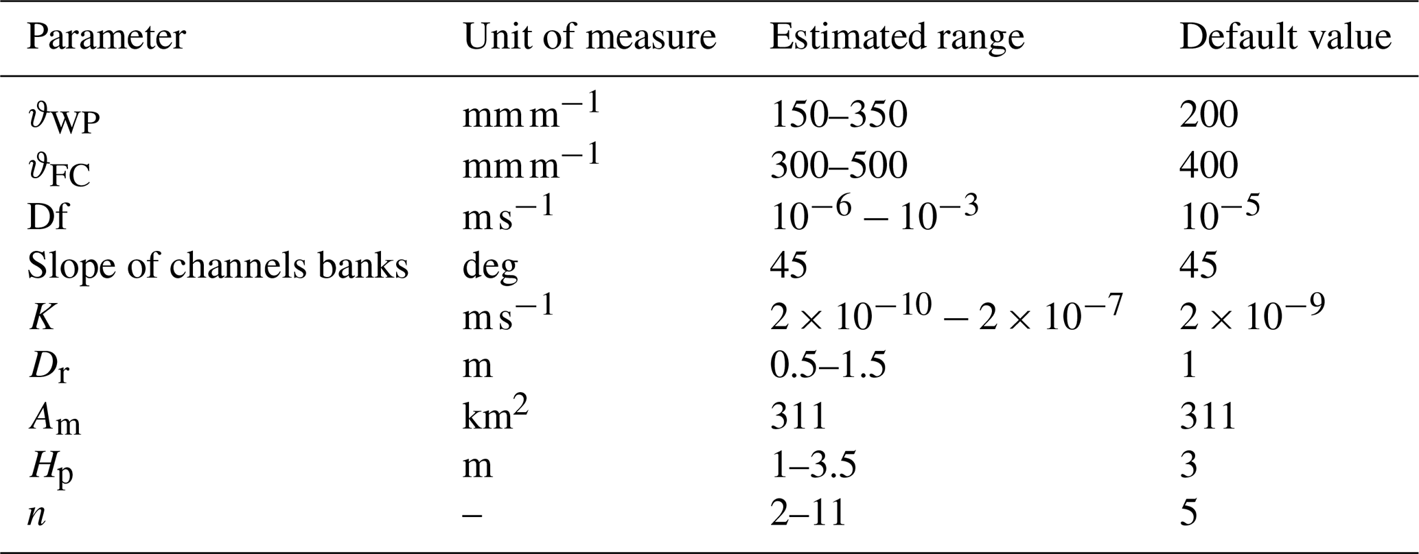
According to the geology of the marshland, with a superficial layer of clays and a deeper layer of alluvial sands and gravels (García Novo and Marín Cabrera, 2006), it was possible to research soil moisture thresholds in the literature (Allen et al., 1998, Chapt. 8, Example 36) and through the use of software for identifying soil water characteristics given their composition. According to these sources for the ϑ_WP a range of 150–350 mm m⁻¹ was considered while ϑ_FC lies in a range between 300 and 500 mm m⁻¹. For the lateral drainage factor (Df) the range of values between 10⁻⁶ and ${\mathrm{10}}^{-\mathrm{3}}\mathrm{m}{\mathrm{s}}^{-\mathrm{1}}$ has been chosen, according to the average properties of the marshland's system, already used in other mathematical models (Serrano Hidalgo, 2023). For the marshland subsoil hydraulic conductivity (K), depending on the type of soil (Shackelford, 2013) a spectrum of values ranging between $\mathrm{2}\times {\mathrm{10}}^{-\mathrm{10}}$ and $\mathrm{2}\times {\mathrm{10}}^{-\mathrm{7}}\mathrm{m}{\mathrm{s}}^{-\mathrm{1}}$ has been set. Considering the presence of a clay soil and the vegetation that composes the marshland, the range of values chosen for the root length parameter (D_r) is 0.5–1.5 m, consistent with standard values for herbaceous and wetland vegetation (Feddes et al., 2001) and coherent with the shallow groundwater conditions and seasonal regime of Doñana (Serrano et al., 2006). Other parameters, depending exclusively on the geometry of the model, were chosen as follows for modelling simplicity: H_p varies between 1 and 3 m while the number of linear channels in the system was varied from 2–11. The marshland area A_m, assumed square for simplicity, was not varied as it is known from technical reports (Sánchez Navarro et al., 2009), literature sources (Paredes Losada, 2020; Aldaya et al., 2010) and available data (such as soil use maps). Similarly, the slope of channels banks is assumed to be 45° for modeling simplicity. Table 2 provides full details on the parameters, and includes the “default values”, i.e. reference values for conducting the sensitivity analysis.

3 Results

This section presents a sensitivity analysis of the model parameters, together with a description of the calibration and validation procedures. The main outputs of WetMAT are then reported, followed by a preliminary application to climate change scenarios.

3.1 Sensitivity analysis

This paragraph explores the sensitivity of each parameter in relation to the various dynamics simulated by the model. Through sensitivity analysis, we assess to what extent each parameter influences the different processes and identify which parameters have the most significant impact on each dynamic.

This sensitivity analysis is fundamental as it supports the calibration of parameters, detailed afterwards. It has allows breaking down the model into components that can be analysed individually, to increase awareness of model limits and sources of uncertainty. We refer, in the following, to three key output variables, namely: the maximum annual flooded area (max MFA) [km²] of the marshland, the mean hydroperiod [d yr⁻¹] of the marshland and the average annual flooded surface of channels Ap (m²) variable, this one, which draws attention to the Channel Water Balance. A univariate sensitivity analysis was performed, varying each parameter within its range using regular intervals. The other parameters were set to their default value (see Table 2). The marshland model has been run using precipitation [mm] and temperature [°C] daily data in the period from 1979–2018, recorded in the “Palacio de Doñana” meteorological station by EBD-CSIC. From these data the daily ET [mm] has been obtained using Hargreaves–Samani approach (Hargreaves and Samani, 1985). Sensitivity analysis was conducted on all parameters and Fig. 4 represents the sensitivity of the selected output variables to parameters where the sensitivity is greatest, referring to the 25th, 50th and 75th percentile of the analysed sample.

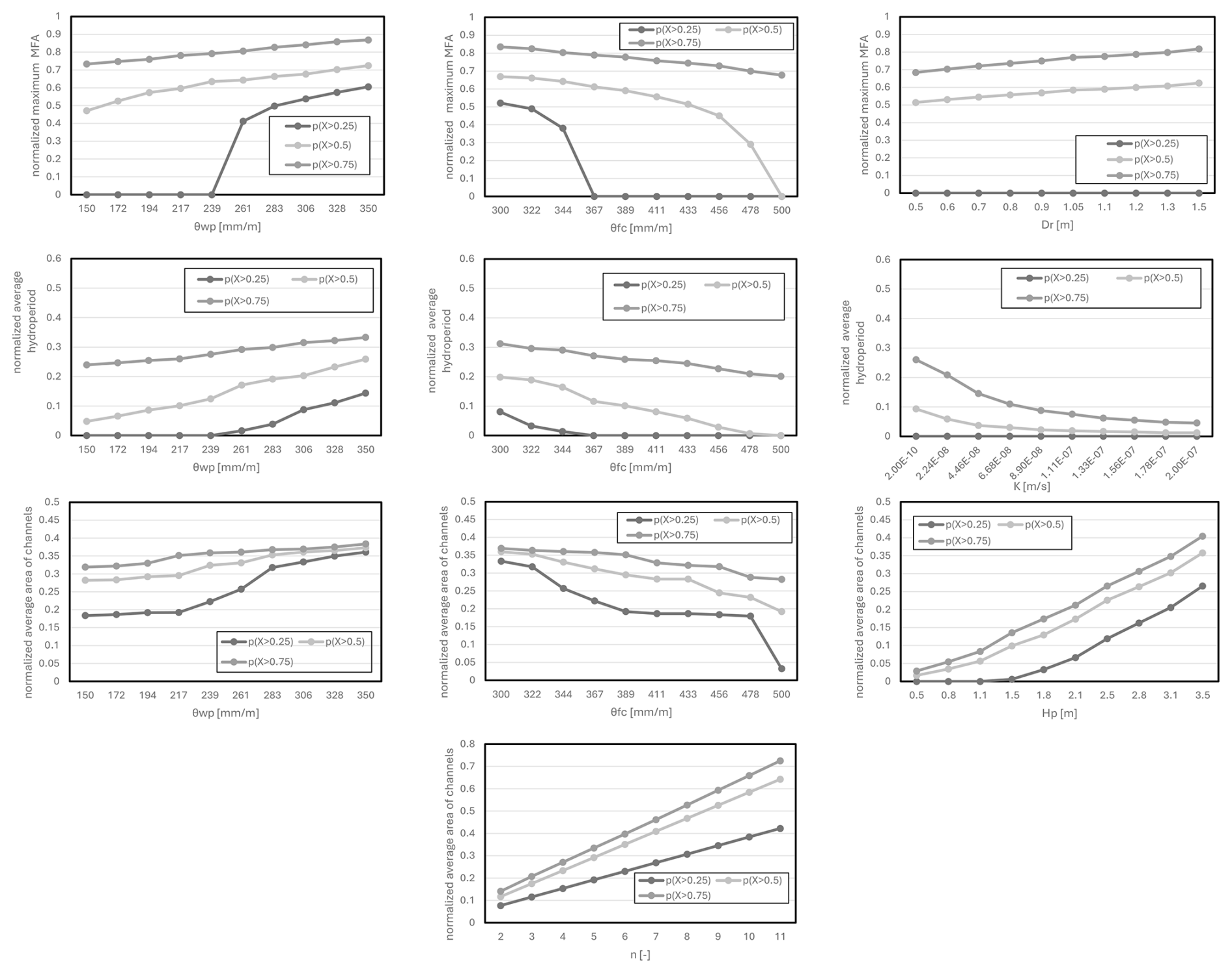
Figure 4 Sensitivity analysis for most sensible model parameters in the evaluation of annual maximum MFA, average hydroperiod and annual average area of channels.

More specifically, Fig. 4 shows the impact of parameters on the maximum MFA, normalized by the total marshland area, on the average hydroperiod normalized by the number of days per year, on the average area of channels normalized by its maximum value found in simulations performed (1 200 000 m²).

Regarding the maximum MFA, parameters related to soil moisture thresholds (ϑ_WP, ϑ_FC) certainly have an interesting trend particularly for low values. The (X>0.25) percentile shows a significant “threshold” trend in both cases (for values placed in the middle of the chosen range) and in the case of ϑ_FC this behaviour is also consolidated for the median. The ϑ_WP parameter is directly proportional to the increase of the flooded area while for high values of ϑ_FC the flooded area decreases, as the soil is supposed to absorb great amounts of water. Moreover, the relevant difference between three percentiles can be, in this case, attributed to the climatic variability of the area in terms of precipitation and evapotranspiration. The model is quite insensitive to the variation of Df, H_p and n, which are the main hydrogeomorphologic parameters of the model. This is not surprising, as the annual maximum flooding occurs when the channels are already full and the area above is uniformly flooded. A limited sensitivity to K and D_r is in this case also observed: as expected, when the hydraulic conductivity increases, the maximum flooded area decreases. Regarding the hydroperiod output, a different perspective is observed, as it focuses on environmental needs over time rather than in space, indicating how many days per year the marshland is flooded. The model shows again a relevant sensitivity to soil moisture parameters (ϑ_WP, ϑ_FC). Compared to MFA, a lower dispersion of data can be noticed, and the changes in system behaviour are less abrupt. Furthermore, the relationship between parameters and the average hydroperiod does not have a clear transition based on a threshold. The model sensitivity to H_p, n and D_r is almost negligible, thus highlighting a limited relevance of hydrogeomorphologic characteristics. A considerable dispersion of data for a variable number of channels is evident: this occurs because the change of geometry contributes to create a different system in every simulation, thus with a different response to daily climatic outputs.  Interestingly, Df and K have a limited impact on the dispersion of values, but a high sensitivity (in particular for K) for low values within the selected range. Regarding the channels area, also in this case, the moisture related parameters (ϑ_WP, ϑ_FC) are highly relevant, yet with a minor data dispersion compared to MFA and hydroperiod. It's also important to note that both ϑ_WP and ϑ_FC exhibit a significant variability in relation to the changes in their values, compared to the other parameters analysed for the same process. The variable is completely insensitive to Df, K and D_r. Conversely, H_p and n play a central role in the process of flooding and emptying of channels. The drainage velocity (lateral and vertical) does not play a central role, but hydrogeomorphological parameters have great sensitivity in this process: the normalized flooded area of the channels varies from 0–0.4 for the parameter H_p, and from 0.15–0.8 for the parameter n; the data dispersion is minimal, and this indicates that the whole sample shows no exceptions. There is direct proportionality between variables and outputs. The summary of the results of the sensitivity analysis is qualitatively proposed in Table 3. Basically, the selected outputs show a high sensitivity to parameters concerning the soil moisture, so a careful calibration is needed. The divergent trends observed for these parameters are consistent with fundamental soil physics (Seneviratne et al., 2010). Specifically, an increase in field capacity (ϑ_FC) enhances the soil's water retention capacity, thereby reducing flooding through increased storage within the control volume. Conversely, a higher wilting point (ϑ_WP) leads to a contraction of the available water for vegetation, inducing a premature cessation of evapotranspirative fluxes. This condition maintains a higher residual water content within the soil profile, facilitating rapid saturation during subsequent meteorological events and consequently increasing the MFA.Conversely the lateral drainage factor shows a very limited impact. Concerning the other parameters, each output shows a different sensitivity. Interestingly, n and H_p (hydrogeomorphologic parameters) for the first two outputs have no sensitivity, but the output of the average channel area is strongly dependent on them.

Table 3 Qualitative results of sensitivity analysis for all processes simulated with the model.

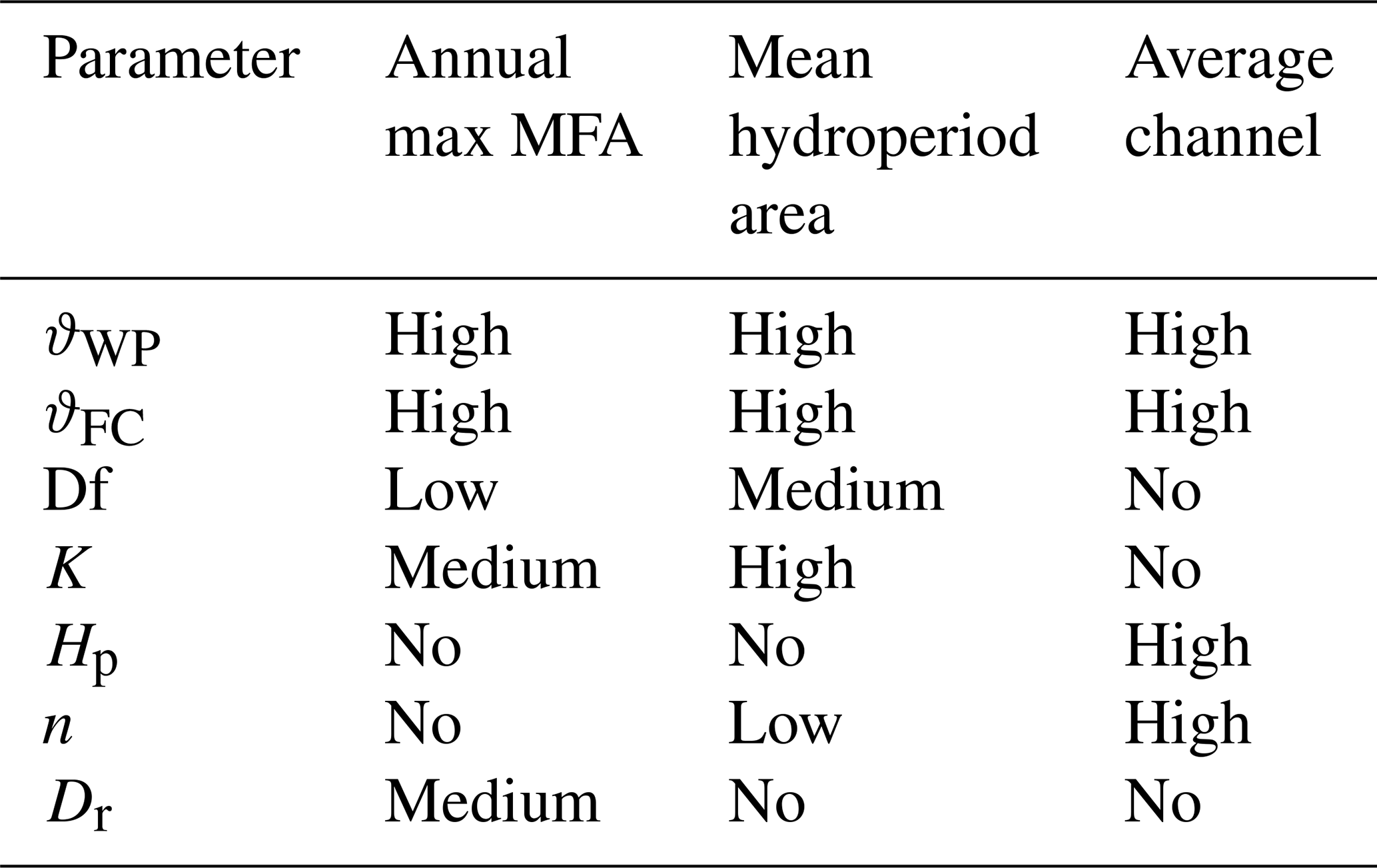
Noteworthy is also the case of the depth of the root zone, which affects only the maximum flooded area even if it is located below the system so it might expect influence on the other processes.

3.2 WetMAT calibration and validation

The present section deals with model calibration and validation, which has been performed comparing model outputs (annual maximum flooded area MFA) with observed data. Reference was made to observed data from the 1980–1981 hydrological year to 2017–2018 (Green et al., 2024). Figure 5 summarizes the main steps in the calibration and validation processes of the WetMAT model, described in further details afterwards.

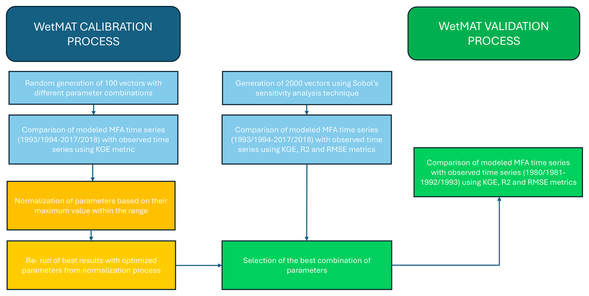
Figure 5 Main steps involved in the calibration and validation processes of the WetMAT model.

The calibration process followed two parallel pathways, which were combined only when selecting the best parameter set to be adopted for the validation stage. On the one hand, calibration relied on the generation of 100 random simulations (Monte Carlo) where all parameters varied within their range except those related to marshland area and slope of channels that were kept constant. On the other hand, a Sobol' sequence approach (Sobol', 1967) was employed as a quasi–Monte Carlo technique to generate 2000 parameter sets, providing a more space-filling sampling of the parameter domain than purely random draws. The outputs from all simulations were compared against observations using three complementary metrics, so as to account for both performance and error aspects (Althoff and Neiva Rodrigues, 2021). Specifically, R² and Kling–Gupta Efficiency (KGE) metrics were adopted as performance metrics, whereas Root Mean Square Error (RMSE) was used as an error metric. The R² metric, although simpler and more intuitive, primarily reflects the model's ability to reproduce the observed variability and is mainly informative with respect to timing; however, it is not sensitive to systematic bias and therefore provides limited insight into volumetric errors, which nonetheless remain relevant. Complementarily, the composite KGE metric is widely regarded as a reference standard in hydrological modelling (Liu, 2020) and has also been considered preferable to other compound measures such as NSE (Thiemig et al., 2013). KGE (Gupta et al., 2009) enables the simultaneous assessment, through separable components, of correlation, bias, and variability. RMSE quantifies the typical magnitude of the simulation error in the same units as flooded area, facilitating a direct physical interpretation. It complements KGE and R² by emphasizing large deviations and by providing an absolute measure of accuracy. The historical time series used for the calibration phase spans from the 1993–1994 hydrological year to the 2017–2018 hydrological year for the MFA variable. An additional analysis on random generated vectors was then performed to further support model calibration: the ten high-ranked simulations in terms of KGE for the maximum flooded area were analysed, normalizing the parameters with respect to the maximum value in the range. All parameters chosen within these simulations were in the middle of their range except the value of K that fell in the lower bound of its range. The ten best random simulations have been therefore re-run, replacing the K value with its extreme value. This choice is consistent with the predominantly clayey soil texture; therefore, adopting a very low hydraulic conductivity is appropriate. Exploring even lower values is unlikely to be informative, because the literature-informed lower bound already renders the corresponding loss term effectively negligible in the water balance. As a result, higher values of KGE (0.85) were obtained for the maximum flooded areas. The final calibrated parameter set, selected by jointly considering the three performance/error metrics for the top-ranked parameter vectors generated through the two parallel calibration approaches, is reported in Table 4 and was subsequently used for WetMAT simulations. Figure 6a shows the comparison between observed and simulated values of maximum MFA. The validation phase of the WetMAT model involved comparing historical time series of the maximum MFA variable, specifically the series generated by the WetMAT model with that from Green et al. (2024), covering the period from the 1980–1981 hydrological year to the 1992–1993 hydrological year. Although the available time series is too short for a fully robust long-term assessment, a commendable KGE value of 0.73 was achieved. Figure 6b shows results of the validation process.

Table 4 Calibrated vector for WetMAT model.

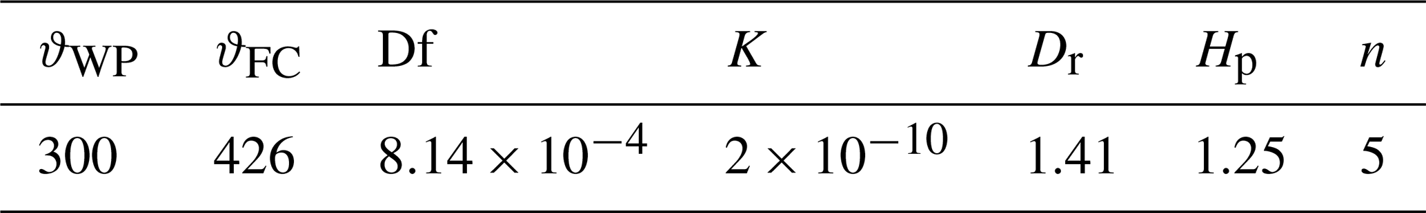
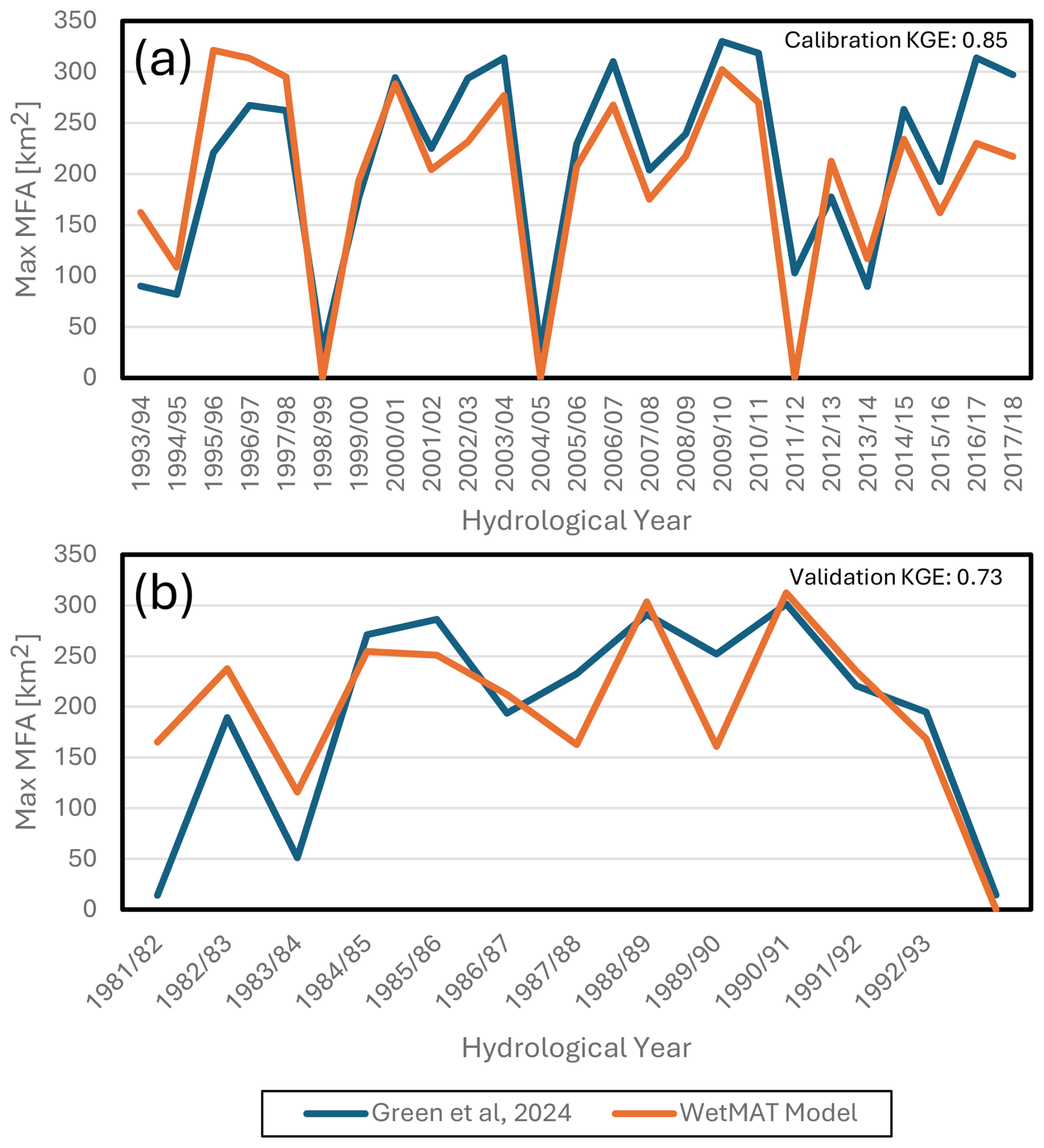
Figure 6 Panel (a) shows the WetMAT model calibration according to the “maximum MFA” variable. Panel (b) shows the WetMAT validation according to the “maximum MFA” variable.

The resulting performance was interpreted against threshold values commonly adopted in general hydrological model evaluation, for which these metrics were originally developed. Accordingly, model performance can be classified as “good” for KGE both during calibration and in the subsequent validation, consistent with the criteria reported in Thiemig et al. (2015). Similarly, the model shows good R² performance in both calibration and validation, as established in the literature (Moriasi et al., 2015).

3.3 WetMAT outputs

The main output of the WetMAT model is the MFA calculated on a daily scale, that allows also the generation of the hydroperiod of the marshland. Data relating to the hydroperiod are available in the literature (Diaz-Delgado et al., 2016) but are calculated differently, following a pixel-based approach unlike how they are calculated in this study, considering the marshland as a single pond, according to a lumped approach whereby the hydroperiod in this case is given by the number of days in which an MFA value different from zero is observed. Some examples are shown in Fig. 7 where the recorded rainfall is represented as well. More specifically, Fig. 7a shows the hydrological year 2005–2006, that can be considered a dry year, as the precipitation value (468.3 mm) is close to 25th percentile of the analysed series (440.25 mm). Figure 7b instead refers to the hydrological year 2006–2007, i.e. a wet year, as the precipitation value (716.9 mm) is the closest to the 75th percentile in the analysed series (1992–1993, 2017–2018). Figure 7c then represents the output of the model over an average hydrological year (2014–2015), characterized by a total annual rainfall of 531.85 mm. The flooding period obtained through WetMAT generally begins in Autumn and ends in late Spring and, despite a high variability, it is consistent with literature evidence (Bustamante et al., 2009; Serrano et al., 2006).

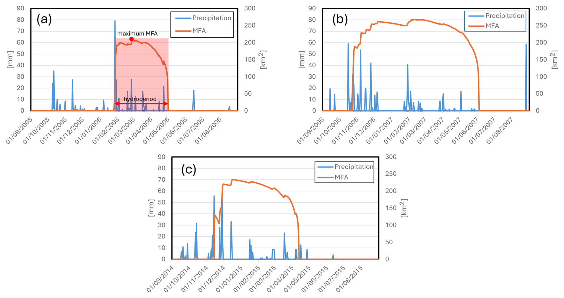
Figure 7 Panel (a) shows the daily plot of flooded areas in hydrologic year 2005–2006 taken as representative of dry year. Panel (b) shows the daily plot of flooded areas in hydrologic year 2006–2007 taken as representative of wet year. Panel (c) represents flooded areas in hydrologic year 2014–2015, taken as representative of an average hydrologic year. All panels show daily precipitation during the hydrologic year.

As previously discussed, the MFA variable generated from WetMAT facilitates both spatial and temporal analysis of flooding dynamics in the marshland. While the hydroperiod and maximum annual MFA are somehow correlated, there is no evidence of mutual dependency, and therefore is essential to consider both variables when assessing marshland state. The importance of incorporating both temporal and spatial characteristics in hydro-ecological studies has been widely acknowledged (Peng et al., 2022; Coleman et al., 2015), particularly in the context of temporary wetlands (Rawat et al., 2025), where ecosystem functioning depends on the joint role of flooded extent and duration. To provide a single, decision-oriented indicator that can synthesizes these two dimensions, the Inundation Persistence Index (IPI) is introduced, assumed as key metric of this study. For each hydrological year, IPI is defined as the product of maximum MFA and the hydroperiod, (expressed as [km² d⁻¹]). By construction IPI can reach high values only when inundation is both extensive and long-lasting, whereas it approaches zero when flooding is limited in the spatial or temporal aspect. While the present formulation is aimed at inter-annual comparisons within the study site, useful specifically for scenario-based assessments, a natural extension of IPI would be a dimensionless, normalized version to facilitate comparisons across different Mediterranean wetlands. This composite variable can be also easily graphically represented (see Fig. 7a for reference). The analysis of the time series of the IPI variable with annual rainfall (proposed in Fig. 8) shows that IPI is equal to or very close to zero in all years with cumulate precipitation below the threshold of 400 mm yr⁻¹ (identified empirically as the transition range separating years with negligible inundation from years with persistent inundation). Figure 8 shows also that, once annual precipitation exceeds 400 mm yr⁻¹, IPI increases with precipitation, indicating a precipitation-controlled regime.

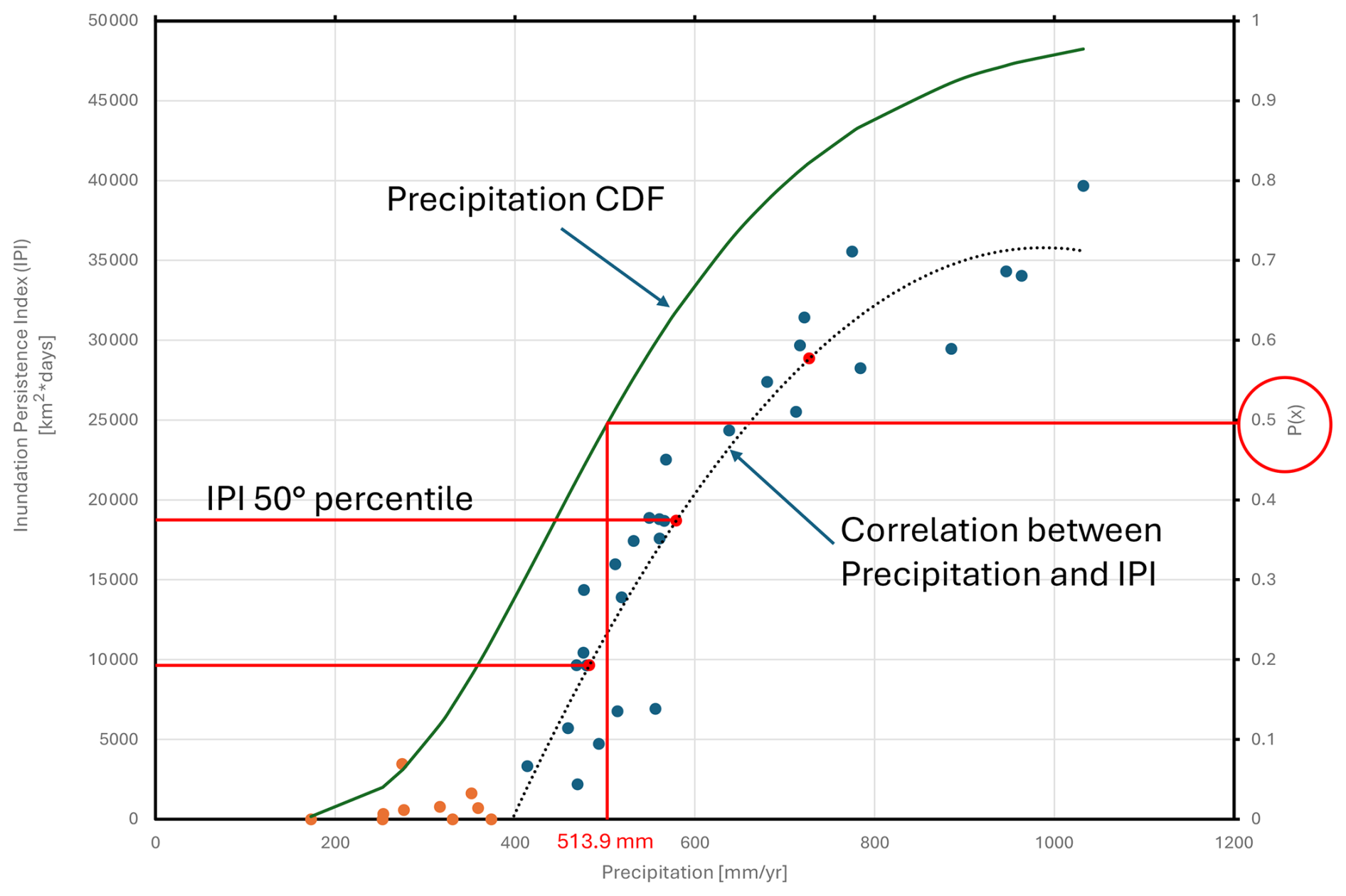
Figure 8 Precipitation log-normal CDF and correlation between Precipitation and Inundation Persistence Index (IPI).

Figure 8 proposes a direct comparison between the precipitation CDF curve and the curve relating the IPI to the precipitation time series. Importantly, “typical” inundation conditions should be interpreted conditionally on inundation occurrence, rather than by directly mapping central tendency metrics of the full precipitation record to inundation metrics.

This implies that even an average year (in terms of rainfall), represented by a rainfall of 513.9 mm yr⁻¹, does not necessarily correspond to typical inundation conditions, and marshland flooding may not occur. When the ecosystem requires extra water supplies, especially during drought years as indicated by the IPI, this would imply management interventions that are beyond the scope of the present work, as WetMAT results are intended to provide hydrological inputs for the design of more complex management scenarios requiring separate, detailed assumptions and analyses. In practice, such interventions could include limiting agricultural groundwater withdrawals and reallocating part of the saved volume to controlled wetland inundation, and/or supplying water from external sources (inter-basin transfers or releases from adjacent artificial reservoirs).

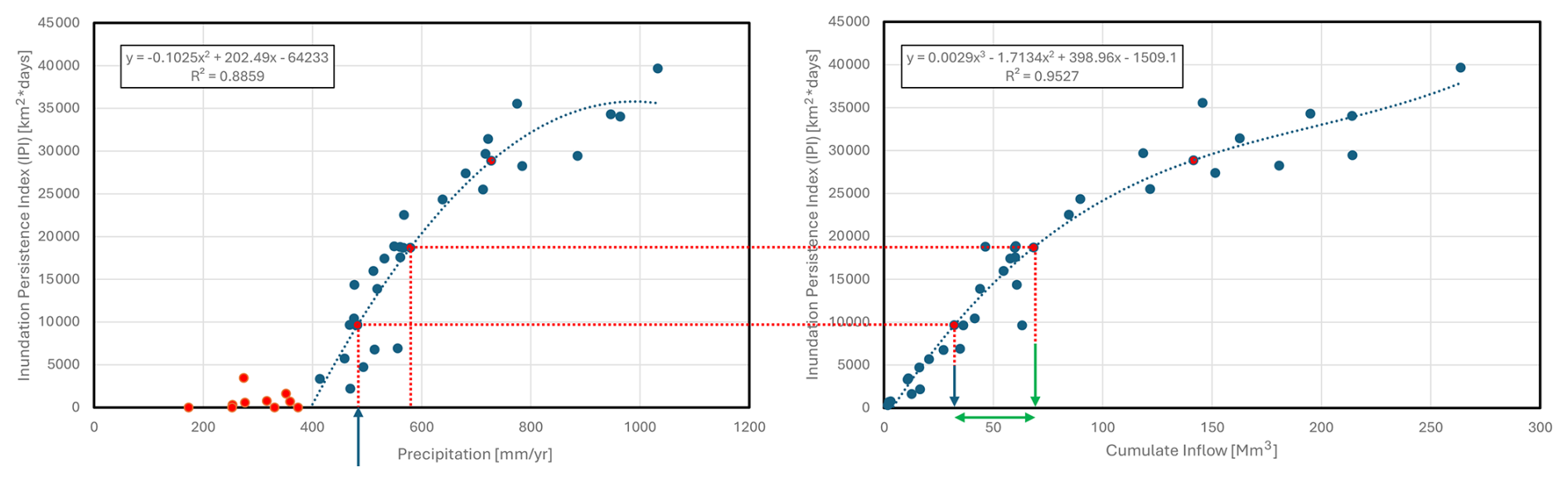
To quantify the amount of water needed by the marshland to reach its average flooding conditions, the correlation between precipitation and IPI and then between the IPI and the cumulate water inputs generated by precipitation on the marshland, namely the Cumulate Inflow (Mm³), are determined. This is shown in Fig. 9 using both a second-degree equation (R²=0.89) and a third-degree equation (R²=0.95). Those equations could be used to estimate, on a yearly basis, how much water is needed beyond precipitation for marshland flooding.

Figure 9 Determination of annual water inputs to the marshland.

3.4 Preliminary WetMAT applications under climate change scenarios

WetMAT can be easily used to model several scenarios, including those related to climate change. Two “representative concentration pathways” (RCP), namely RCP 4.5 and RCP 8.5 (van Vuuren et al., 2011), are analyzed. The climate projections used as forcing in this section were obtained from PRIMA LENSES project datasets and here adopted as external inputs for the model. Daily precipitation and 2 m air temperature data were taken from the Copernicus Climate Change Service (C3S) and, specifically, from the CORDEX regional climate projections database (C3S, 2019), which provides dynamically downscaled simulations from Global Climate Models (GCMs) to Regional Climate Models (RCMs) under the EURO-CORDEX framework. Within the LENSES project, an ensemble approach was adopted in which multiple RCMs driven by different CMIP5 GCMs (Coupled Model Intercomparison Project Phase 5) were used to represent climate-model uncertainty. For the Doñana domain (with coordinates 37.8–36.8° N and 6.9–6.0° W used), the dataset has daily temporal resolution and 5 km spatial resolution for both precipitation and mean temperature. Importantly, for these two variables a bias-adjusted EURO-CORDEX dataset was adopted: the daily precipitation and temperature ensemble was bias-adjusted using EFAS-Meteo as reference and a bias-adjustment method developed by the Swedish Meteorological and Hydrological Institute (SMHI). Evapotranspiration data (ETP) are calculated starting from temperature data using the Hargreaves–Samani formula.

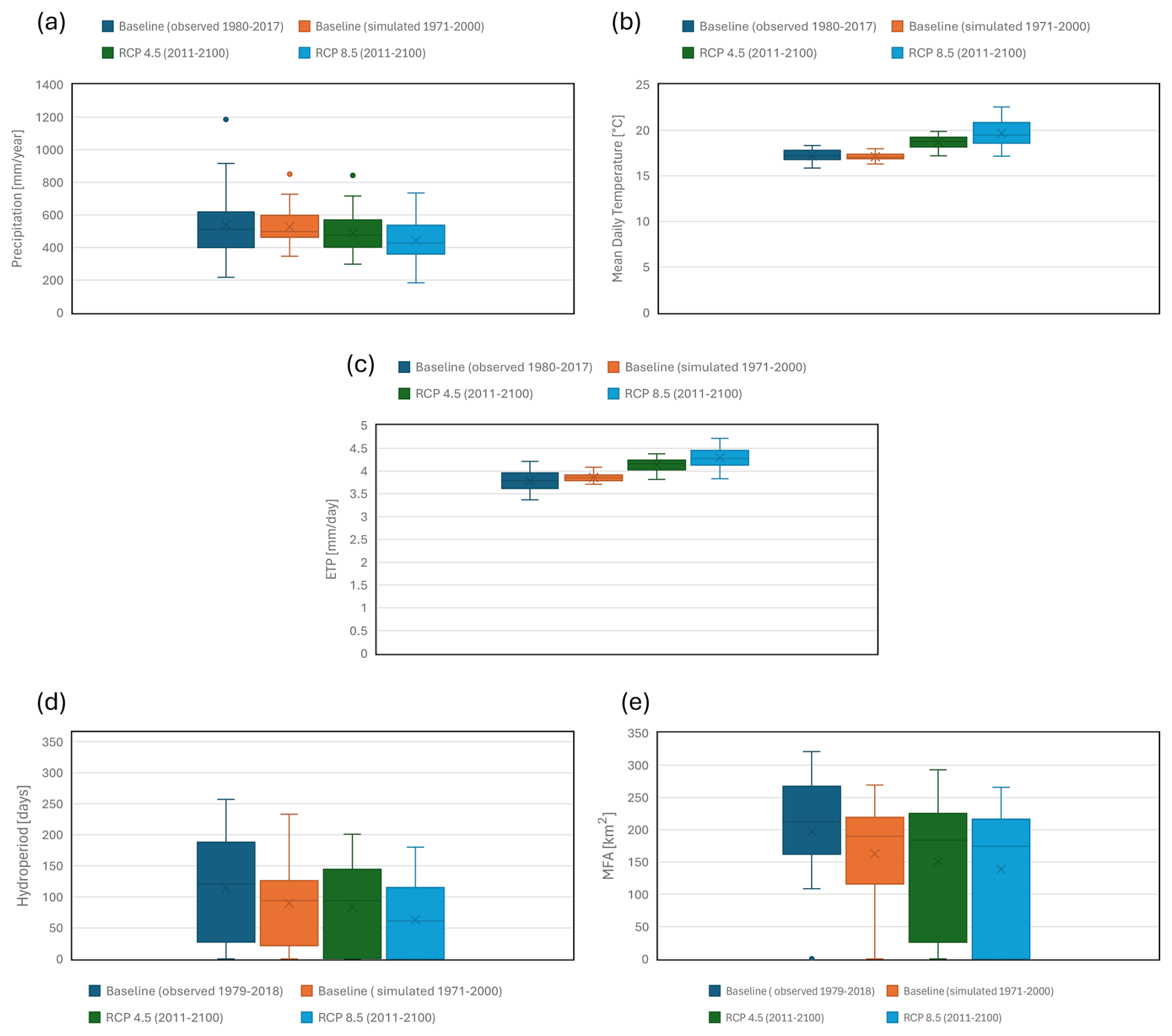
Figure 10 Boxplot representing the evolution of Precipitation variable (a), Mean Daily Temperature variable (b), ETP variable (c). Panel (d) represents the evolution of Hydroperiod variable in climate change scenarios and panel (e) represents the evolution of maximum Marshland Flooded Area (MFA) variable in climate change scenarios.

Figure 10a–c present the results related to climate change scenarios for the three climatic variables used in the WetMAT model: Precipitation, Mean Daily Temperature, ETP. Reference is made to four data series, namely: (i) “Baseline (observed)” with observed data for the period 1980–2017, (ii) “Baseline (simulated)” scenario (1971–2000); (iii) RCP4.5 scenario simulated over the period 2011–2100; (iv) RCP 8.5 scenario simulated over the period 2011–2100.

As observed when comparing the performance of the boxplots for the three variables, precipitation exhibits greater variability (Kim and Onof, 2020). This variability notably influences the future scenarios, which show a higher degree of uncertainty compared to the observed ones. In contrast, the other two variables analysed show less variability in the projections, and therefore less uncertainty. However, there is still a significant increase in the average values, with a rise of 2.2 °C in the average temperature. ETP, being temperature-dependent, follows the same trend as temperature.

The results of the WetMAT model referred to the two main processes of the marshland, namely the MFA and the hydroperiod are presented in Fig. 10d and e, using the same scenarios described above. In WetMAT, these descriptors of flooding conditions are controlled by the balance between precipitation inputs and atmospheric demand. Accordingly, the projected increase in temperature and the associated increase in ETP reduce the effective water availability and provide a mechanistic explanation for the simulated decrease in both hydroperiod and MFA, with stronger impacts under RCP 8.5. Conversely, the high variability of precipitation mainly contributes to the uncertainty of the projections rather than providing a single dominant directional driver.

Figure 10 shows that the variability of variables (in particular MFA) greatly increases in climate change scenario. Results show a potential worsening of marshland's conditions with a general decrease of the extension of flooded areas and a decrease of the hydroperiod.

4 Discussions

This section details to what extent the present study answered the research questions formulated in the Introduction and highlights limitations and potential replicability of the WetMAT tool.

First, despite the complexity of the temporary Doñana wetland and the simplifications introduced in WetMAT, the tool can satisfactorily reproduce the flooding and drainage dynamics of the wetland, achieving a good match with the observed data in terms of MFA. Details on model calibration and validation are presented in Sect. 3.2.

Second, concerning the role of WetMAT for supporting hydro-ecological assessment, the comparative analysis of Fig. 7, highlights differences between the different hydrological years in terms of MFA and hydroperiod. It is important to emphasize that in the analysed period, the wettest and driest years occurred in consecutive years. This is a clear example of the considerable interannual climate variability in the area, and subsequent complexity in system state assessment. Furthermore, as Fig. 7a clearly shows, it should be noted that despite the rainy season may start long before the beginning of marshland flooding, the flooding takes place only after particularly intense rainfall (approximately exceeding 50 mm). Figure 10 show an analysis performed focusing on climate change scenarios, which indicate a potential deterioration in the wetland condition over time.

The second research question is closely linked to the third, that focuses on the use of WetMAT to support decision-makers. In this regard, the use of a new parameter, i.e. the Inundation Persistence Index IPI that resumes the hydrological response of the wetland to climate, proves to be valuable. This index integrates information provided by the MFA and the hydroperiod and allows determining the environmental water requirements of the wetland for each hydrological year and assessing how much water must be added from external sources to maintain the wetland in a state of average flooding. Indeed, as observed in Fig. 8, an average annual rainfall leads to a flooding consistency effect that slightly exceeds the 25th percentile of the IPI series, a straightforward calculation of environmental water requirement is essential for decision-makers. Going further into details, the analysis proposed expresses a statistical view of the yearly water supply needed by the wetland to achieve an average flooding condition, based on the entire historical dataset, that is 25.2 Mm³. To get a tangible quantitative comparison, this volume is approximately to 25 % of the current annual groundwater withdrawals for agricultural purposes (100 Mm³) although this estimate is subject to significant uncertainty due to unrecorded illegal usages (Green et al., 2024; Acreman and Salathe, 2022; UNESCO, 2020). In summary, the use of WetMAT could be useful for planning mitigation and restoration measures aimed at ensuring sustainable future scenarios, need which is widely acknowledged (CHG, 2022; Guardiola Albert and Jackson, 2011).

The main limitation of the WetMAT model relates to the challenges in finding all the necessary data for implementation, which contribute to highlight the relevance of the careful review of the “grey literature” performed in the Doñana case study. As reported in Green et al. (2024) the streamflow gauges of surface watercourses do not have complete time series. Similarly, although gates exist for the surface drainage of the marshland, they are not gauged and therefore it is impossible to derive information related to its discharges. As for the ecotones and the levels of groundwater, there are reports of their dramatic drops and decreases but there is no reliable information about their possible contributions to the wetland. However, the rationale behind WetMAT is to keep the model as simple as possible, although this may introduce simplifications such as the use of precipitation as the only input for the wetland, or a limited treatment of outflows.

Regarding the use of IPI, one of the main findings of this work, a potential development of this proposed key metric concerns its transferability across sites. The current IPI is intentionally parsimonious and physically interpretable, but its magnitude may still reflect site-specific attributes (e.g., the maximum floodable area). For comparative studies across different Mediterranean wetlands, a promising avenue is to formulate a dimensionless, normalized IPI, so that values are not dominated by differences in absolute scale. This could be achieved, for instance, by normalizing maximum inundation extent by a site-specific reference and expressing hydroperiod as a fraction of days within the hydrological year, yielding an index bounded in [0,1] and directly comparable across systems. The hydroperiod variable is used for the implementation of IPI, as it is recognised that this is a factor that describes the hydrological response of the marshland. However, as already specified, one limitation of the study is the difficulty of comparing the hydroperiod observed in the literature with that described in this study, due to conceptual differences in the calculation of this variable. Furthermore, the available data on the maximum MFA, derived from the literature, lacks indications on when it occurs during the year. Despite these limitations, it is important to highlight the applicability and replicability of WetMAT across various temporary and non-temporary wetland contexts, as these wetlands are already commonly classified in a way that allows for their modelling to be as similar and efficient as possible once a system is implemented (Toronto and Region Conservation Authority, 2020). The model simplicity, with a limited number of parameters and a straightforward description of processes, makes it suitable for diverse settings.

5 Conclusions

The present work describes an innovative hydrological balance model (WetMAT), that can be used to describe the dynamic evolution of a temporal marshland through his outputs (MFA, hydroperiod). The model is based on a straightforward mathematical modelling, on a daily basis, of the main hydrological processes that contribute to the generation of flooding, starting from simple and relatively easy to find climate data as daily precipitation and daily average temperature. WetMAT has been developed and tested in the Doñana wetland case study but can be easily adapted to be replicated elsewhere, thanks to the low number of parameters required to use the model, its computational simplicity, and, most importantly, given the need to identify water requirements in such at-risk environments where estimation and planning of environmental needs are necessary.

Future steps in the progression of this work involve the use of agent-based modelling to evaluate and quantify the effectiveness of WetMAT outputs within an integrated decision-making context (Giordano et al., 2024). Additionally, the model will be applied to other case studies, similar in climatic conditions but differing in terms of scale or the types of components involved, in order to assess the true scalability and replicability of WetMAT.

A process to identify the environmental demand is necessary and essential in any context water conflicts persist among different users and the vision of Nexus is pursued: the simple modelling of WetMAT has shown that this is possible.