A hybrid Kolmogorov–Arnold Networks-based model with attention for predicting Arctic river streamflow

Arctic rivers represent important components of the Arctic and global hydrological and climate systems, serving as dynamic conduits between terrestrial and marine environments in some rapidly changing regions. They transport freshwater, sediments, nutrients, and carbon from vast watersheds to the Arctic Ocean and affect ocean circulation patterns and regional climate dynamics. Despite their importance, modeling Arctic rivers remains challenging because of sparse data networks, unique cryospheric dynamics, and complex responses to hydrometeorological variables. In this study, a novel hybrid deep learning model is developed to address these challenges and predict Arctic river discharge by incorporating Kolmogorov–Arnold Networks (KAN), Long Short-Term Memory, and the attention mechanism with seasonal trigonometry encoding and physics-based constraints. It integrates several novel components: (1) A KAN-based deep learning component learns and captures intricate temporal patterns from nonlinear hydrometeorological data; (2) Explicit physical constraints designed for the characteristics of permafrost-dominated watersheds govern snow accumulation and melt processes through the architectural design and loss function; (3) Seasonal variations are accounted for using trigonometry functions to represent cyclical patterns; (4) A residual compensation structure allows the proposed model to revisit systematic errors in initial predictions and helps capture complex nonlinear processes that are not fully represented. The Kolyma River, which is dominated by permafrost, is adopted to test the performance of the newly developed model. It obtains more robust and accurate predictive performance compared to baseline models. The role of physical constraints, the residual compensated architecture, and the trigonometry encoding are assessed by ablation analysis. The results indicate that these components improve the predictive performance. This novel approach offers a new pathway for addressing key challenges of hydrological forecasting in cold, permafrost-dominated regions and provides a robust framework for improving Arctic river discharge prediction.

1 Introduction

Arctic rivers are integral to the Arctic's hydrological cycle and global climate systems and have undergone significant changes in recent years (Rawlins and Karmalkar, 2024). They are essential for transporting vast amounts of freshwater, sediments, and organic matter from terrestrial sources to the Arctic Ocean and sustaining the biodiversity of the region and supporting unique ecosystems (Tank et al., 2023; Liu et al., 2025; Vonk et al., 2025). The intricate connections between Arctic rivers and other cryospheric and atmospheric components make them highly sensitive to climate change (Feng et al., 2021). The response to climatic shifts, including changes in precipitation patterns, temperature regimes, snowmelt timing, and evapotranspiration rates in Arctic watersheds, has far-reaching implications for ecosystem stability and introduces significant uncertainties into future climate projections (Peterson et al., 2002).

Predicting hydrodynamics of Arctic rivers remains challenging due to the region's unique environmental conditions, data scarcity, complex feedback mechanisms, and their nonlinear responses to temperature, rainfall, and evapotranspiration. For example, warming temperatures can accelerate permafrost thaw and alter hydrological cycles in Arctic regions. Temperature thresholds play a crucial role, particularly around the 0 °C mark, where phase changes in precipitation and surface water create abrupt shifts in river dynamics (Prowse et al., 2011; Walvoord and Kurylyk, 2016). These temperature-dependent transitions are further complicated by permafrost thawing, which destabilizes riverbanks, modifies groundwater flow paths, changes groundwater-surface water interactions, and increases sediment and nutrient loads, creating intricate feedback loops and complicates flow predictions (McClelland et al., 2004; Wang et al., 2021).

Over the last several decades, significant efforts have been directed towards forecasting the responses of river discharge to hydrometeorological conditions and understanding the underlying driving mechanisms (Gelfan et al., 2017; Jin et al., 2024a; Wang et al., 2021; Zhang et al., 2023; Zhou and Zhang, 2023a). These approaches can be broadly categorized into process-based models and empirical models. Process-based models simulate detailed physical and chemical processes within hydrological systems. For example, Gelfan et al. (2017) employed process-based hydrological models, including the HYdrological Predictions for the Environment (HYPE) and ECOlogical Model for Applied Geophysics (ECOMAG), to simulate the hydrodynamics of the Lena and Mackenzie Rivers and assessed the impacts of climate change. Similarly, Krogh et al. (2017) developed a physics-based hydrological model that accounted for key hydrological processes for quantifying water losses at the tundra-taiga transition in a small Arctic basin. While these process-based approaches provide valuable insights into the underlying hydrological processes and mechanisms, their successful implementation usually requires extensive parameterization and detailed characterization of environmental conditions, such as topography, spatially distributed hydrological parameters, and vegetation patterns. Such comprehensive data requirements pose significant challenges in Arctic regions, where remote locations, limited infrastructure, and harsh climatic conditions constrain field measurements and sustained monitoring campaigns (Gao et al., 2020). In contrast, empirical models, particularly data-driven approaches, focus on establishing direct mappings between input and output variables without requiring comprehensive understanding of the underlying hydrological systems (Zhou and Zhang, 2022b).

Recently, data-driven models have been increasingly developed and used to simulate hydrodynamics and characterize hydrological systems in Arctic regions. For instance, Zhang et al. (2023) simulated the streamflow changes of several major Arctic rivers with meteorological conditions using a Support Vector Regression model. This machine learning model was then used to estimate responses of these rivers to the elevated temperature and precipitation conditions. Singh et al. (2020) implemented several convolutional neural networks models (CNN), including UNet, SegNet, Deeplab and DenseNet, to estimate surface concentration of river ice. Their approach demonstrated improved estimation performance compared to existing methods by addressing the key challenge of noise and errors in the limited available training data. Sergeev et al. (2024) developed a hybrid model integrating wavelet transform with long short-term memory (LSTM) networks for predicting Arctic methane concentration with greenhouse gases data monitored from the Belyy Island in Russia.

Despite these advances, significant challenges remain in modeling intricate river systems. Current deep learning approaches often struggle to capture complex and nonlinear relationships between meteorological variables and river discharge (Jin et al., 2024b; Zhou et al., 2024a). To improve the performance with nonlinear data such as rainfall-runoff relationship, many technologies have been developed. For example, Basu et al. (2022) proposed a nonlinear autoregressive model with exogenous variables for flood prediction in Ireland. Bakhshi Ostadkalayeh et al. (2023) used Kalman Filter (KF) to manage nonlinear systems and improve LSTM performance for forecasting streamflow. Zhou et al. (2024b) integrated the ensemble empirical model decomposition technology with temporal fusion transformers and developed a new hybrid deep learning model for discharge prediction, which outperformed baseline models. Liu et al. (2024) proposed Kolmogorov–Arnold Networks (KAN) based on the theoretical foundation in the Kolmogorov–Arnold theorem. Unlike traditional neural networks that use fixed activation functions, the KAN model parameterized learnable activation functions on the connections between nodes, which enhances the model's capacity to capture complex nonlinear relationships in data. Beyond predictive skill, unlike conventional MLPs with fixed node activations, KANs parameterize learnable univariate functions on edges, enabling direct visualization and interrogation of the learned input–output relationships (Liu et al., 2024). This property makes KANs attractive in hydrology, where model usefulness includes both accuracy and ability to extract physically meaningful patterns from data.

In addition, the scarcity of training data in Arctic regions limits the generalization of traditional deep learning models, leading to less satisfying performance (Alzubaidi et al., 2023). Physics-informed neural networks (PINN) and physics-guided deep learning approaches offer a promising solution by incorporating physical constraints and domain knowledge into the learning process (Karniadakis et al., 2021). By embedding physical laws into the loss function, these hybrid approaches can improve prediction accuracy while ensuring physically consistent results (Zhong et al., 2024). A variety of physics-informed deep learning models have been developed and demonstrated promising results in various hydrological applications. For example, Yang et al. (2020) proposed a hydrological model that integrated the physical process with a machine learning model for simulating daily streamflow. This hybrid model obtained accurate predictions for long-term daily streamflow with limited training data and demonstrated the effectiveness of this approach for reducing data requirements. Xie et al. (2021) integrated physical mechanisms into a deep learning model through both modified loss functions and synthetically generated training samples for forecasting streamflow. Their model outperformed traditional models and highlighted the value of incorporating physical constraints into deep learning frameworks for hydrological modeling.

To address these challenges and improve predictive performance in permafrost-dominated Arctic rivers, a novel residual compensated physics-informed KAN-LSTM with attention model (RCPIKLA) that integrates seasonal patterns, physics-based constraints, KAN, LSTM and attention is proposed for forecasting Arctic river discharge in this study. This newly proposed model introduces several key innovations that serve specific purposes: (1) a KAN-based deep learning model coupled with LSTM and the attention mechanism, which enables sophisticated feature representation and temporal patterns recognition for nonlinear hydrometeorological data; (2) physical constraints that explicitly govern snow accumulation and melt processes, which improve physical consistency through the architectural design and loss function; (3) a residual compensation structure that combines a physics-informed main network with a specialized residual network, which allows the model to capture physically governed patterns and local anomalies; and (4) a temporal pattern recognition system that incorporates cyclical encoding of seasonal features for seasonal variations. This integrated approach is specifically designed to address the challenges of hydrological forecasting in cold, permafrost-dominated regions, where snow accumulation and melt play a crucial role in seasonal discharge patterns. The innovative components are integrated to enhance its predictive accuracy, physical consistency, and ability to handle complex seasonal dynamics and hydrological processes that characterize Arctic river systems.

2 Study area and data acquisition

To assess its performance, the newly developed model is tested on the Kolyma River located in the northeaster Siberia (Fig. 1). The Kolyma River is one of the major Arctic rivers with a mean annual discharge of 136 km³ yr⁻¹ and the largest river system draining into the East Siberian Sea. The Kolyma watershed is Earth's largest watershed that is 100 % underlain by continuous permafrost (Holmes et al., 2012). The extensive permafrost coverage makes the Kolyma watershed particularly sensitive to climate warming, leading to its unique hydrological behaviors (Spencer et al., 2015). With a drainage basin of approximately 647 000 km², the Kolyma River flows through diverse landscapes including the Kolyma Mountains, permafrost regions, and tundra ecosystems. The river's discharge regime is characterized by a distinctive seasonal pattern, with peak flows occurring during the spring snowmelt period (May–June) and low flows during the winter months when the river is ice-covered (Bring et al., 2016).

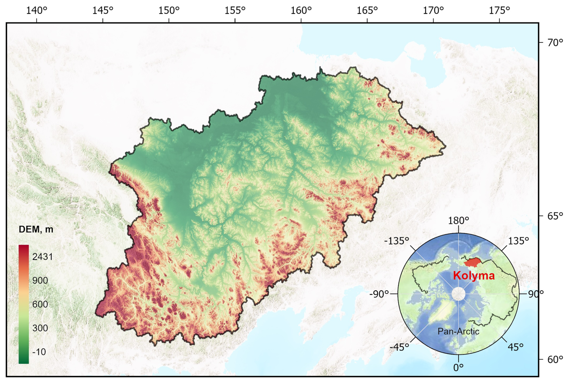
Figure 1 The geographic location and topography of the Kolyma catchment.

In this study, monthly temperature (T), precipitation (P) and potential evapotranspiration (PET) are used as input variables for forecasting discharge values of the Kolyma River. The Kolyma discharge records (1978–2020) at the Kolymsk gauge station (68.73° N, 158.72° E) are obtained from the ArcticGRO Discharge Dataset Version 20231204 (https://arcticgreatrivers.org/data, last access: 5 September 2025). Note that the historical discharge data of the Kolyma River is not used as input variables in this study, which allows the model to establish direct relationships between hydrometeorological drivers and river discharge without incorporating autoregressive components, thereby focusing specifically on how climatic factors influence discharge patterns in permafrost-dominated watersheds. Gridded monthly average 2 m temperature and potential evapotranspiration with a resolution of 0.5° are obtained from CRU TS v. 4.07 (Harris et al., 2020). Additionally, monthly precipitation data at a 0.5° resolution are obtained from the Global Precipitation Climatology Centre (GPCC) dataset (Schneider et al., 2022). The complete dataset spans from January 1978 to December 2020, which is partitioned into training (80 %) and testing (20 %) datasets for model development and performance assessment.

3 Methodology

3.1 Kolmogorov–Arnold Networks

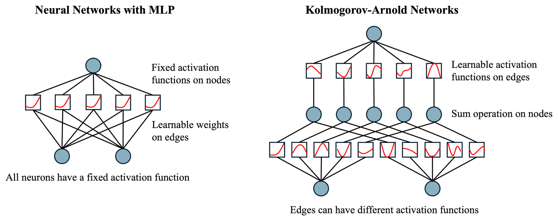
In the Kolmogorov–Arnold representation theorem, it states that any continuous multivariate function can be represented as a superposition of continuous functions of a single variable (Kůrková, 1992). Based on this theoretical foundation and the mechanism of decomposing the multivariate function into various univariate functions, the Kolmogorov–Arnold Networks model (KAN) was developed by replacing all weight parameters with univariate functions parameterized as splines, rather than using Multi-Layer Perceptrons (MLPs) in traditional neural networks, as illustrated in Fig. 2 (Liu et al., 2024). This structure allows the KAN model to dynamically adapt its processing to various aspects of the data and emphasize finer details by modulating the granularity of these splines (Granata et al., 2024). With learnable activation functions and structured transformations, it can effectively extract nonlinear relationships and capture intricate patterns, making it well-suited for modeling complex hydrological systems like Arctic river discharge.

Figure 2 The structure of Kolmogorov–Arnold Networks (KAN) compared to MLP.

In this newly developed hybrid model, the KAN module is used as an advanced feature transformation block and a nonlinear feature extractor that processes raw hydrological and meteorological inputs before the sequential modeling stage. The architecture of the KAN module is composed of several parts: (1) Input expansion: the raw input features including precipitation, temperature and evapotranspiration are first projected into a higher dimensional space by a fully connected layer that increases the representational capacity. The dimension expansion of the input features allows the model to isolate some nonlinear interactions between variables, such as temperature-driven snowmelt thresholds or precipitation-phase transitions; (2) Nonlinear activation: a Gaussian Error Linear Unit (GELU) activation is then applied to the expanded features. The GELU function introduces smooth nonlinearity and enables the network to capture intricate patterns in the input data, which approximates the role of univariate functions in the Kolmogorov–Arnold theorem while avoiding the computational overhead of spline optimization; (3) Dimensionality reduction: a second linear layer then compresses the activated features down to a lower-dimensional space which is then fused with physics-based constraints, such as snowpack dynamics and fed into the LSTM-Attention network for temporal integration. It aims at effectively distilling the information into a compact, yet expressive representation that is more amenable for subsequent processing. The KAN transformation and processing steps can be expressed as the following equations accordingly:

$$\begin{array}{}\text{(1)}& {\displaystyle }{H}_{\mathrm{1}}={\mathbf{W}}_{\mathrm{1}}X+{\mathit{b}}_{\mathrm{1}},\text{(2)}& {\displaystyle }{H}_{\mathrm{2}}=\text{GELU}\left(H_{\mathrm{1}}\right),\text{(3)}& {\displaystyle }\text{KAN}\left(X\right)={\mathbf{W}}_{\mathrm{2}}{H}_{\mathrm{2}}+{\mathit{b}}_{\mathrm{2}},\end{array}$$

where X is the input features; W₁ and W₂ refer to the expansion and compression weight matrices; b₁ and b₂ are the corresponding bias vectors; GELU is the Gaussian Error Linear Unit activation function.

3.2 Long Short-Term Memory

Following the Kolmogorov–Arnold transformation, the processed input features will enter the Long Short-Term Memory (LSTM) module. LSTM is a modified variant of recurrent neural networks (RNNs), specifically designed to address the vanishing gradient problem while learning long-term dependencies in sequential data (Hochreiter and Schmidhuber, 1997). By incorporating the gating mechanism and a hidden state, the LSTM model can efficiently regulate information flow through the network and selectively remember or forget information in long sequences. Because of its ability to capture temporal dependencies inherent in river systems, the LSTM model has been widely used in a variety of hydrological models (Gao et al., 2020; Zhou and Zhang, 2023b). It aims at learning and identifying important historical patterns in meteorological variables (such as temperature and precipitation) that influence current river discharge, while simultaneously recognizing the varying time lags between these inputs and their hydrological responses. This capability makes LSTMs especially suitable for modeling Arctic river systems, where discharge patterns are influenced by both immediate meteorological conditions and longer-term processes such as snowmelt and permafrost dynamics (Kratzert et al., 2018).

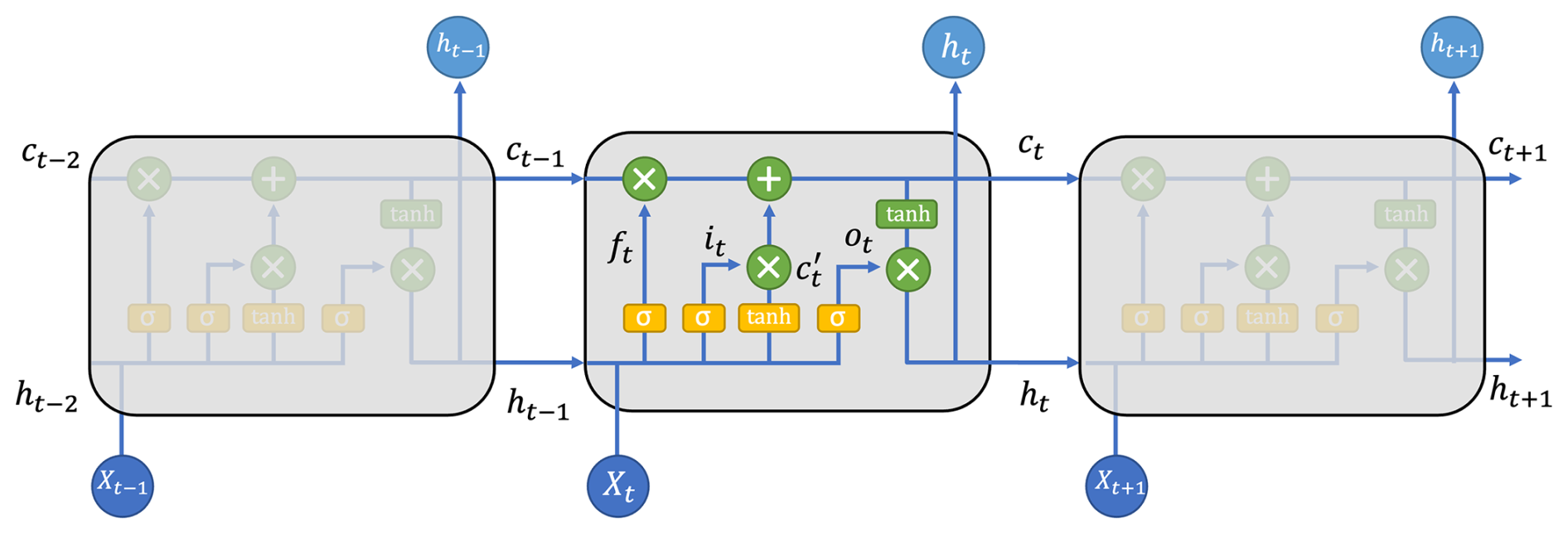
As illustrated in Fig. 3, the memory cell of each repetitive LSTM block is primarily composed of three gates: the input gate (i_t), forget gate (f_t), and output gate (o_t). The input gate determines which new information should be stored in the cell state. The forget gate decides what information should be discarded from the previous cell state. The output gate controls how much of the cell state should be exposed to the next layer. This gating mechanism allows LSTMs to maintain and update relevant information over long sequences while filtering out irrelevant details (Hochreiter and Schmidhuber, 1997). At any time step t, the hidden state (h_t) and the cell state (c_t) are calculated based on the previous hidden state (h_t−1) and cell state (c_t−1) with three logic gates as follows:

$$\begin{array}{}\text{(4)}& {\displaystyle }{f}_t=\mathit{\sigma }(W_{\mathrm{f}}{X}_t+U_{\mathrm{f}}{h}_{t-\mathrm{1}}+b_{\mathrm{f}}),\text{(5)}& {\displaystyle }{i}_t=\mathit{\sigma }(W_{\mathrm{i}}{X}_t+U_{\mathrm{i}}{h}_{t-\mathrm{1}}+b_{\mathrm{i}}),\text{(6)}& {\displaystyle }{c}_t^{\prime }=\tanh (W_{\mathrm{c}}{X}_t+U_{\mathrm{c}}{h}_{t-\mathrm{1}}+b_{\mathrm{c}}),\text{(7)}& {\displaystyle }{c}_t=f_t\otimes c(t-\mathrm{1})+i_t\otimes c_t^{\prime },\text{(8)}& {\displaystyle }{o}_t=\mathit{\sigma }(W_{\mathrm{o}}{X}_t+U_{\mathrm{o}}{h}_{t-\mathrm{1}}+b_{\mathrm{o}}),\text{(9)}& {\displaystyle }{h}_t=o_t\otimes \tanh \left(c_t\right),\end{array}$$

where c_t, $c_t^{\prime }$, and h_t are the cell state, candidate cell state, and hidden state at time step t, respectively; X_t refers to the input variables processed by the KAN module; W, U and b are weight matrices and bias vectors whereas subscripts f, i, c, and o denote the forget gate, input gate, candidate cell, and output gate; σ and tanh are the sigmoid and hyperbolic tangent activation functions; ⊗ is the element-wise operation.

Figure 3 The architecture of the LSTM model.

3.3 Attention

A global attention mechanism is incorporated into the LSTM component of the newly proposed model to assign different importance weights to past time steps when making predictions, which enables the model to dynamically weight and aggregate information across temporal sequences. As the influence of historical conditions on current discharge exhibits complex temporal dependencies in hydrological modeling, the attention mechanism can help capture both short-term fluctuations and long-range interactions in input variables. The attention score for each time step can be computed as (Vaswani et al., 2017):

$$\begin{array}{}\text{(10)}& {\displaystyle }{e}_t={\mathit{v}}^T\tanh (W_{\mathrm{a}}{h}_t+b_{\mathrm{a}}),\text{(11)}& {\displaystyle }{\mathit{\alpha }}_t={\displaystyle \frac{\exp \left(e_t\right)}{{\sum }_j\exp \left(e_j\right)}},\text{(12)}& {\displaystyle }\mathit{C}={\sum }_t{\mathit{\alpha }}_t{h}_t,\text{(13)}& {\displaystyle }\widehat{Q}=W_{\mathrm{c}}\mathit{C}+b_{\mathrm{c}},\end{array}$$

where W and b denote weight and bias parameters; e_t refers to the attention score at time step t; h_t is the hidden state from the LSTM component at time step t; v is a learnable vector which determines the importance of each hidden state; α_t is the attention weight; C is the context vector that represents a weighted sum of all hidden states; $\widehat{Q}$ refers to the predicted discharge.

3.4 Physics-informed mechanisms

Physics-informed neural networks improve hydrological modeling by combining established physical information with deep learning architectures, which creates a synergistic approach that leverages the strengths of both methodologies. In this study, a hybrid physics-informed approach is implemented through two complementary mechanisms: (1) a dedicated snowpack layer directly integrated into the model architecture, and (2) a physics-constrained loss function. The snowpack layer explicitly simulates snow accumulation and melting processes based on temperature and precipitation. It tracks precipitation falling as snow when temperatures drop below freezing (T<0 °C, where T represents temperature) and computes snowmelt using a temperature-dependent rate function (Hock, 2003):

$$\begin{array}{}\text{(14)}& M_{\mathrm{r}}=f_{\mathrm{m}}\cdot max(T,\mathrm{0}),\end{array}$$

where M_r is the melting rate, and f_m is the melting factor coefficient. The melting factor of 0.5 $\mathrm{mm}\mathrm{°}{\mathrm{C}}^{-\mathrm{1}}{\mathrm{d}}^{-\mathrm{1}}$ is adopted in this study based on empirical studies of Arctic snowpack dynamics (Hock, 2003). The snowpack mass balance is estimated as follows (DeWalle and Rango, 2008):

$$\begin{array}{}\text{(15)}& S_t=S_{t-\mathrm{1}}+P_t^{\text{snow}}-M_t,\end{array}$$

where S_t and S_t−1 denote the snowpack water equivalent at time t and t−1; M_t is the actual snowmelt, which is calculated as $M_t=min(S_{t-\mathrm{1}},M_{\mathrm{r}})$; $P_t^{\text{snow}}$ refers to the snowfall fraction of precipitation, which is determined by the following equation (Harpold et al., 2017):

$$\begin{array}{}\text{(16)}& P_t^{\text{snow}}=\left\{\begin{array}{ll}{P}_t,& \text{if}T<\mathrm{0}\mathrm{°}\mathrm{C}\\ \mathrm{0},& \text{otherwise}\end{array}\right.,\end{array}$$

where P_t is the precipitation rate. The initial values of snow storage and melt are set as zero at the beginning. An architectural innovation is that the calculated snowmelt amount is directly added to the data-driven neural network output before the final activation function of the first stage as shown in Fig. 2, creating a hybrid prediction that leverages both physical understanding and learned patterns:

$$\begin{array}{}\text{(17)}& \widehat{Q}=\text{ReLU}\left(Q_{\text{LSTM}}+M_t\right),\end{array}$$

Where ${\widehat{Q}}_i$ and Q_LSTM are the predicted discharge from the first stage and the output from the LSTM with attention component, respectively; ReLU refers to rectified linear unit activation function. In addition to the snowpack layer, a physics-constrained loss function is implemented for enforcing physical consistency through the term:

$$\begin{array}{}\text{(18)}& {\mathcal{L}}_{\text{phys}}={\displaystyle \frac{\mathrm{1}}{n}}{\sum }_{i}max(M_t-{\widehat{Q}}_i,\mathrm{0}),\end{array}$$

where n is the number of samples, and ℒ_phys refers to the physics-constrained loss function term. This term penalizes physically inconsistent predictions where the modeled discharge is less than the calculated snowmelt contribution.

The calculated snowmelt contribution is one of the major contributors to the discharge rate in permafrost-dominated watersheds, such as the Kolyma River. While instantaneous discharge can legitimately fall below melt rates due to transient storage in the active layer, evapotranspiration losses, or refreezing during diurnal temperature fluctuations, these effects become negligible at the monthly aggregation scale in large, permafrost-dominated basins like the Kolyma River (Gusev et al., 2015). Continuous permafrost covering >90 % of the Kolyma basin severely restricts subsurface infiltration and groundwater storage (Walvoord and Kurylyk, 2016; Woo et al., 2008). Unlike temperate watersheds where snowmelt can recharge deep aquifers, the impermeable permafrost layer forces meltwater to travel through the shallow active layer with limited storage capacity. Consequently, snowmelt rapidly converts to surface and near-surface runoff with minimal opportunity for long-term retention (Bring et al., 2016). Also, Arctic rivers such as the Kolyma River and the Lena River exhibit strong discharge seasonality characteristic, with the majority of the annual discharge occurring during summer months (Ye et al., 2003). During these months, snowmelt represents the dominant water source, and the monthly timestep aggregates over 30 d during which daily temperature fluctuations and local-scale heterogeneity in melt timing average out across the entire basin. While refreezing can occur during cold nights or sublimation during clear, windy days, these losses are small relative to the total melt flux at monthly basin-scale aggregation (Suzuki et al., 2015). Therefore, snowmelt represents a dominant and appropriate lower bound on discharge at this spatiotemporal scale (Yang et al., 2002).

The asymmetric physical constraint in this study is designed and implemented to reflect both the availability of data and the scale-dependent hydrology of large permafrost-dominated Arctic watersheds. It is worthwhile to note that implementing symmetric upper bound constraints will further increase the physics-informed condition. Future studies should collect comprehensive data and develop more sophisticated, symmetric physics constraints that fully respect mass conservation while accounting for all water balance components.

In summary, this dual physics-guided approach is particularly valuable for Arctic rivers where seasonal snow accumulation and permafrost melt dominate the hydrological regime. In these regions, river discharge often exhibits complex, threshold-dependent behaviors and memory effects related to temperature-controlled phase changes in water, and processes that statistical models often struggle to capture accurately without explicit physical constraints. By incorporating both a direct snowmelt contribution mechanism and physics-consistency loss penalties, the proposed model maintains physical realism even when data limitations exist.

3.5 Residual compensated mechanism

While the physics-informed deep learning model may improve prediction accuracy by embedding domain knowledge, they may still fail to capture certain discrepancies between observed and predicted discharge values caused by sources, such as model simplifications, missing hydrological processes, noise in the input data, and extreme events. To address this limitation, a residual compensated mechanism is incorporated. As shown in Fig. 2, the residual compensated framework in the newly proposed model operates in a two-stage process. First, we train a physics-informed KAN-LSTM model that incorporates snowpack dynamics and constraints through the combined loss function (ℒ_combined):

$$\begin{array}{}\text{(19)}& {\mathcal{L}}_{\text{combined}}=\mathit{\alpha }{\mathcal{L}}_{\text{MSE}}(\widehat{Q},Q_{\text{obs}})+\mathit{\beta }{\mathcal{L}}_{\text{phys}},\end{array}$$

where ℒ_MSE refers to the mean squared error between the prediction $\widehat{Q}$ and the observation Q_obs; α and β are weighting coefficients that control the relative importance of the data-driven loss (MSE) and physics-informed constraint terms in the combined loss function. These parameters are determined during the model development phase to achieve optimal performance on the testing dataset. In the second stage, the residuals (R_i) between observations and physics-based predictions are computed: $R_i=Q_{\text{obs},i}-{\widehat{Q}}_i$. These residuals represent the information discrepancies that the physics-informed KAN-LSTM model fails to capture. A separate residual model (M_res) which has a KAN-LSTM architecture without physics-informed components is trained to specifically learn the discrepancies: ${\widehat{R}}_i=M_{\text{res}}\left(X_i\right)$. The final discharge prediction (${\widehat{Q}}_{\text{final},i}$) is obtained by combining results from the first and second stage:

$$\begin{array}{}\text{(20)}& {\widehat{Q}}_{\text{final},i}={\widehat{Q}}_i+{\widehat{R}}_i.\end{array}$$

This residual compensated approach has several advantages: on one hand, it preserves the physical consistency by incorporating the physics-informed component during the first stage. On the other hand, the residual prediction in the second stage can focus exclusively on missed patterns and systematic anomalies, creating a specialized representation for complex processes. As a result, it enables end-to-end training where each component focuses on complementary aspects of the hydrological system: the physics-informed deep learning model captures the first-order processes driven by hydrometeorological variables, while the residual model captures secondary influences and complex feedback mechanisms. It is especially beneficial for Arctic river systems, where seasonal transitions and complex cryospheric processes may not be fully captured by simplified physics representations.

3.6 Evaluation metrics

To assess the performance of the proposed model in the Kolyma River, three popular evaluation metrics are adopted in this study: Nash–Sutcliffe Efficiency (NSE), Root Mean Square Error (RMSE) and Kling–Gupta Efficiency (KGE) (Cinkus et al., 2023; Gupta et al., 2009; Zhou and Zhang, 2022a; Kling et al., 2012). NSE is a dimensionless metric widely used in hydrological modeling that measures how well the model predictions match the observed data compared to using the mean of the observations as a predictor (Gupta et al., 2009). An NSE value of 1 indicates a perfect fit, while values approaching zero or negative suggest that the model performs no better than using the mean value of the observed data. The NSE value can be calculated as:

$$\begin{array}{}\text{(21)}& \text{NSE}=\mathrm{1}-{\displaystyle \frac{{\sum }_{i=\mathrm{1}}^n(Q_{\text{obs},i}-{\widehat{Q}}_{\text{final},i}{)}^{\mathrm{2}}}{{\sum }_{i=\mathrm{1}}^n{\left(Q_{\text{obs},i}-\stackrel{\mathrm{‾}}{Q}\right)}^{\mathrm{2}}}},\end{array}$$

where Q_obs,i and $\stackrel{\mathrm{‾}}{Q}$ are the observed discharge value at time step t and the average discharge, respectively. In hydrological modeling, NSE values above 0.75 indicate very good model performance (Moriasi et al., 2007). RMSE is an absolute error metric that quantifies the average magnitude of prediction errors in the original units of discharge being predicted. RMSE gives higher weight to large errors due to its squared terms, which makes it particularly useful for evaluating models where large errors are especially undesirable, such as in flood prediction. Lower RMSE values indicate better model performance, with RMSE=0 representing a perfect fit. It is defined as:

$$\begin{array}{}\text{(22)}& \text{RMSE}=\sqrt{{\displaystyle \frac{\mathrm{1}}{n}}{\sum }_{i=\mathrm{1}}^n(Q_{\text{obs},i}-{\widehat{Q}}_{\text{final},i}{)}^{\mathrm{2}}}.\end{array}$$

In addition to NSE and RMSE, the Kling–Gupta Efficiency (KGE) is employed to provide a balanced assessment of model performance. The KGE metric was developed to address certain limitations of NSE, particularly its sensitivity to extreme values and the potential compensation of errors in mean, variance, and correlation (Gupta et al., 2009). Unlike other metrics, KGE explicitly decomposes model performance into three components: linear correlation, bias ratio, and variability ratio. In this study, the modified KGE is employed, which addresses issues with the original formulation's sensitivity to the magnitude of standard deviations (Kling et al., 2012). The modified KGE (KGE^′) is calculated as:

$$\begin{array}{}\text{(23)}& {\text{KGE}}^{\prime }=\mathrm{1}-\sqrt{{\left(r_{\text{kge}}-\mathrm{1}\right)}^{\mathrm{2}}+{\left({\mathit{\beta }}_{\text{kge}}-\mathrm{1}\right)}^{\mathrm{2}}+{\left({\mathit{\gamma }}_{\text{kge}}-\mathrm{1}\right)}^{\mathrm{2}}},\end{array}$$

where r_kge refers to the linear correlation coefficient between observed and simulated discharge; β_kge refers to the ratio of simulated mean to observed mean; γ_kge denotes the variability ratio. The KGE^′ ranges theoretically from −∞ to 1, with ${\text{KGE}}^{\prime }=\mathrm{1}$ indicating perfect agreement between observations and predictions in terms of correlation, bias, and variability. A KGE^′ value of −0.41 represents the performance of using the mean flow as a predictor, serving as a natural benchmark below which model predictions are no better than simply using the long-term average (Knoben et al., 2019). In hydrological modeling applications, KGE^′ values above 0.75 are generally considered very good, values between 0.5 and 0.75 indicate satisfactory performance, and values below 0.5 suggest unsatisfactory model performance (Towner et al., 2019). The use of multiple complementary metrics (NSE, RMSE, and KGE^′) provides a comprehensive evaluation framework. While NSE emphasizes matching variance and is sensitive to peak flows, KGE^′ provides balanced assessment across correlation, bias, and variability. RMSE quantifies absolute error magnitude in original units, which is particularly important for operational applications. Together, these metrics enable thorough assessment of model performance across different aspects of discharge prediction, from overall pattern matching to peak flow accuracy.

3.7 Model implementation and training

As shown in Fig. 4, prior to model training, the input variables, including monthly precipitation, temperature and evapotranspiration data, are preprocessed and standardized using the Z-score normalization technique: $X_{\text{std}}=\frac{X-\mathit{\mu }}{\mathit{\sigma }}$, where μ and σ are the mean and standard deviation computed from the training dataset; X and X_std denote the input values before and after standardization, respectively. This standardization process ensures that features measured on different scales contribute appropriately during training and facilitates model convergence (LeCun et al., 1998).

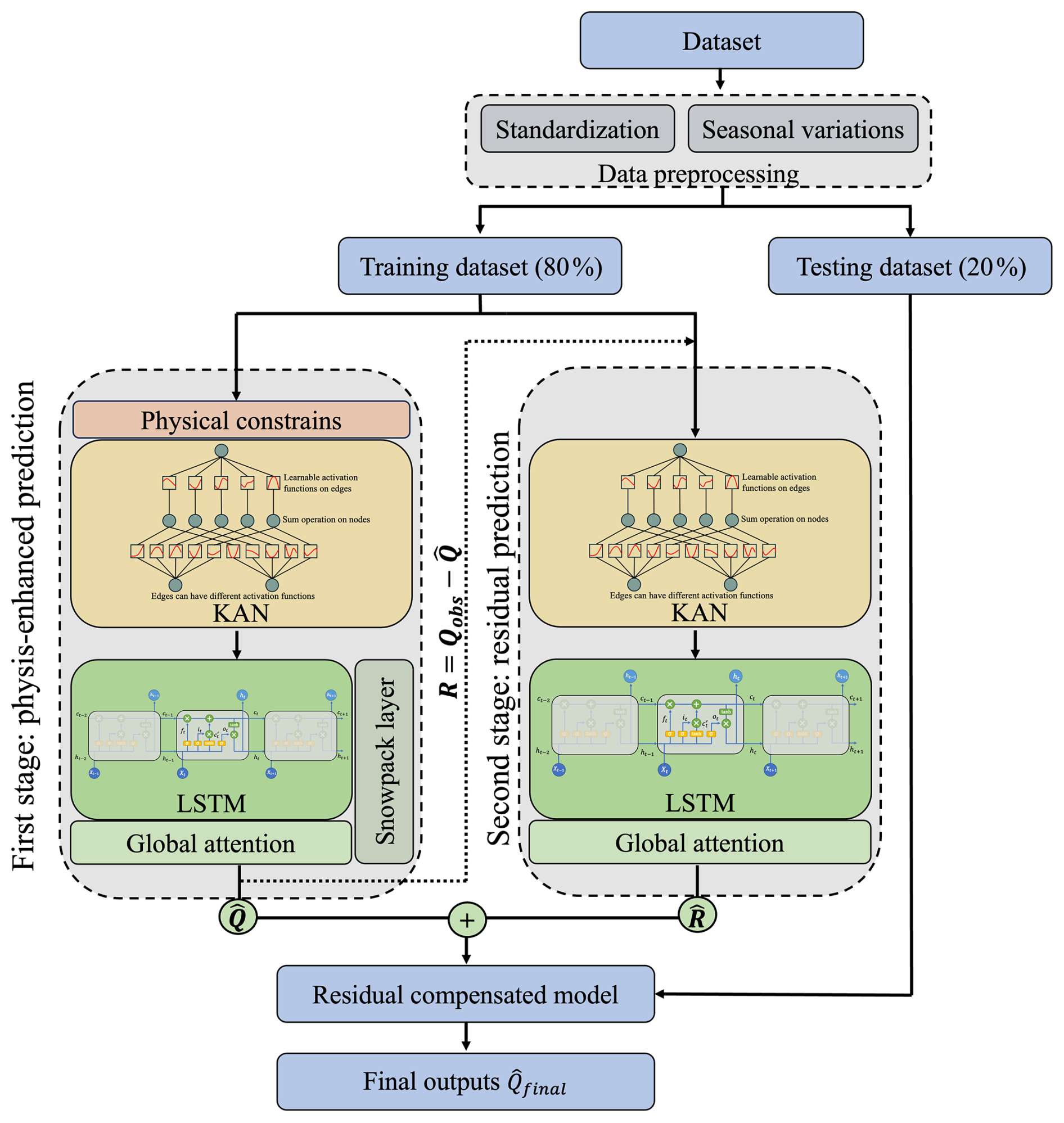
Figure 4 The architecture of the residual compensated physics-informed KAN-LSTM model with attention.

In regions dominated by permafrost, snow accumulation and melt typically exhibit strong seasonal periodicity (Andersson et al., 2021; Ernakovich et al., 2014). Discharge patterns are strongly influenced by annual cycles of temperature, snow accumulation, and melt in Arctic hydrological systems (Häkkinen and Mellor, 1992). Accurately capturing such periodic behaviors can help develop robust long-term forecasting models. To include these cyclical patterns and facilitate smooth temporal transition, a trigonometric encoding (TE) of seasonal features is incorporated as input variables using sine and cosine transformations of the calendar month. Specifically, the timestamp is encoded to two features using the following trigonometric transformations:

$$\begin{array}{}\text{(24)}& {\text{Month}}_{\sin }=\sin \left(\mathrm{2}\mathit{\pi }{\displaystyle \frac{m}{\mathrm{12}}}\right);{\text{Month}}_{\cos }=\cos \left(\mathrm{2}\mathit{\pi }{\displaystyle \frac{m}{\mathrm{12}}}\right),\end{array}$$

where m refers to the calendar month $m\in \mathit{\{}\mathrm{1},\mathrm{2},\mathrm{\dots },\mathrm{12}\mathit{\}}$. These encodings aim at capturing cyclical temporal patterns without introducing artificial discontinuities between December and January. The trigonometric features are concatenated with other input variables, including temperature, precipitation and evapotranspiration, and fed into the residual-compensated physics-informed KAN-LSTM model with attention.

The hyperparameters and configuration settings used in this study are summarized in Table S1 in the Supplement. The choice of hyperparameters balances model capacity with overfitting risk, given the limited training data available. The LSTM hidden dimension of 64 units and a dropout rate of 0.3 prevent overfitting while capturing essential temporal patterns. The batch size and epoch size are set to 32 and 150, respectively. The optimal physics constraint weight (β=0.3) and the MSE weight (α=0.7) are adopted by conducting grid search over $\mathit{\alpha }\in \mathit{\{}\mathrm{0.1},\mathrm{0.3},\mathrm{0.5},\mathrm{0.7},\mathrm{0.9}\mathit{\}}$ (Fig. S1 in the Supplement). With these hyperparameters, the newly proposed model trained in the training dataset of the Kolyma River, and then the fine-tuned models are applied to the unseen testing dataset for the assessment of the predictive performance. The prediction performance is compared with several popular temporal baseline models, including simple RNN, LSTM, and GRU models. Simple RNN is a basic recurrent architecture that processes sequential data by maintaining a hidden state updated at each time step, but it often suffers from vanishing gradients when learning long-term dependencies. LSTM addresses this limitation through its gating mechanisms and a separate cell state, which allows information to persist across long sequences (Hochreiter and Schmidhuber, 1997). GRU simplifies the LSTM architecture by combining the input and forget gates into a single update gate and merging the cell and hidden states, thereby reducing the number of parameters while retaining the ability to model long-range dependencies (Cho et al., 2014). These three recurrent architectures are widely used for sequence modeling and provide meaningful baseline references for assessing the proposed RCPIKLA framework. To assess model stability and minimize the effects of stochastic processes in the training procedure, each model configuration is trained 10 times independently on Google Colab. This repeated training protocol allows assessment of performance variability arising from the inherent stochasticity in the optimization process, including random batch shuffling and numerical precision variations.

Ablation analysis is commonly used to assess the contribution of individual model components (Zhi et al., 2023; Zhou, 2025). In this study, we compare three ablation variants: the complete RCPIKLA model, which incorporates both physics-informed constraints and residual compensation; RCKLA-no physics-informed, which retains the residual structure but excludes the physics-informed constraints; and PIKLA-no residual, which includes the physics-informed constraints but removes the residual compensation structure. Each variant is trained 10 times independently at each forecasting horizon from 1 to 12 months, yielding 120 evaluations per model.

4 Results

4.1 Performance comparison among various baseline models with various time steps

The model performance across different time steps (1–12 months) reveals variations in predictive capabilities among the models tested. Prediction ensemble means and variability across 10 independent training runs at each forecasting horizon are reported in Tables S2–S4. Presented in Fig. 5, it shows the comparison of NSE, RMSE and KGE^′ values for the Kolyma River discharge predictions using several popular baseline models and the newly proposed residual compensated physics-informed KAN-LSTM model with attention. The NSE values demonstrate that the newly proposed RCPIKLA model consistently outperforms all baseline models across all time steps, achieving the highest NSE values ranging from 0.81 to 0.86. This superior performance is particularly obvious at the time step of 9 months, where RCPIKLA reaches peak NSE values of approximately 0.86. The traditional deep learning models, including the simple RNN, GRU, and LSTM models, show similar performance patterns with NSE values ranging between 0.65 and 0.76. These models exhibit a noticeable decline in performance at medium-range time steps (4–8 months), with their lowest NSE values observed around months 5–6, which suggests limitations in capturing seasonal transitions in Arctic river systems. The RMSE analysis corroborates these findings, with RCPIKLA achieving the lowest error values (7.1–8.5 mm) across all time steps. Again, the RCPIKLA model demonstrates lower prediction errors compared to other baseline approaches, which exhibit RMSE values ranging from 9.5 to 11.5 mm. The higher RMSE values for Simple RNN, GRU, and LSTM at medium-range time steps further highlight their difficulties in accurately predicting discharge during critical seasonal transition periods. The KGE^′ metric provides additional insights into model performance by decomposing errors into correlation, bias, and variability components. The RCPIKLA model achieves KGE^′ values ranging from 0.74 to 0.82 across all time steps. Similar to NSE, the RCPIKLA model reaches its peak KGE^′ performance of approximately 0.82 at the 9-month time step. The baseline models demonstrate modest KGE^′ performance, with values ranging from 0.64 to 0.73. A notable degradation in KGE^′ performance is observed at the 12-month time step, where the RCPIKLA value drops to approximately 0.74, falling below the 0.75 threshold. This decline likely reflects the challenges of maintaining balanced performance across all three KGE^′ components (correlation, bias, and variability) at very long forecasting horizons. At 12 months, accumulated prediction errors and the increased difficulty in capturing seasonal phase transitions may cause the model's predictions to exhibit greater bias or variability mismatch compared to observations, despite maintaining reasonable correlation.

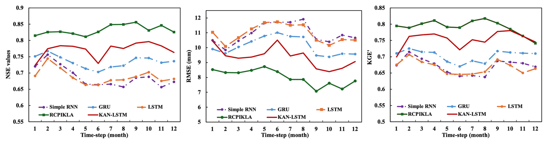
Figure 5 The means of NSE (left), RMSE (middle) and KGE^′ (right) values of 10 independent runs over various time steps. The models include the residual-compensated physics-informed KAN-LSTM model with attention (RCPIKLA), simple RNN, LSTM, GRU and KAN-LSTM.

The optimal performance at the 9-month input sequence length reflects important temporal characteristics of this permafrost-dominated watershed and the model's capacity to capture structured temporal dependencies. In the Kolyma River basin, current discharge is influenced by hydrometeorological conditions that could span multiple seasons, such as snow accumulation, snowmelt dynamics, and subsequent baseflow recession controlled by active layer storage and permafrost-restricted groundwater flows. The 9-month optimal input window captures the information of seasonal dynamics which provides the model with sufficient temporal context. The attention mechanism further refines this by assigning higher importance to specific antecedent months that strongly influence current discharge. Shorter sequences may fail to capture full seasonal cycles and snow accumulation processes, while longer sequences (10–12 months) likely introduce temporal uncertainties.

To complement the mean evaluation metrics, Fig. 6 summarizes the distributions of NSE, RMSE, and KGE^′ values across 10 independent runs for each model architecture. The box plots illustrate the variability and stability of model performance and provide insight into model robustness and generalization ability. The RCPIKLA model demonstrates the best overall performance with the highest median NSE, lowest median RMSE, and highest median KGE^′ along with the narrowest interquartile range. This indicates not only high accuracy but also low variability across runs, suggesting a stable learning and prediction process. Regarding NSE and RMSE, outliers are less frequent and less extreme for RCPIKLA, which indicates a consistently reliable model output. LSTM and Simple RNN exhibit wider interquartile ranges in all metrics' distributions. This means higher sensitivity to random initialization and potential overfitting or underfitting in different runs. GRU shows moderately better consistency than LSTM and Simple RNN but still falls short of the stability achieved by RCPIKLA. RCPIKLA's KGE^′ distribution (0.78–0.82) shows clear separation from the baseline models, with minimal distribution overlap. This distinct separation in KGE^′ performance, combined with greater NSE and lower RMSE, confirms that the newly proposed RCPIKLA model obtains accurate prediction performance, and outperforms other baseline models. These results demonstrate that incorporating physical constraints with the KAN-LSTM model and complementing them with residual learning significantly improve predictive performance for capturing complex patterns in Arctic river discharge.

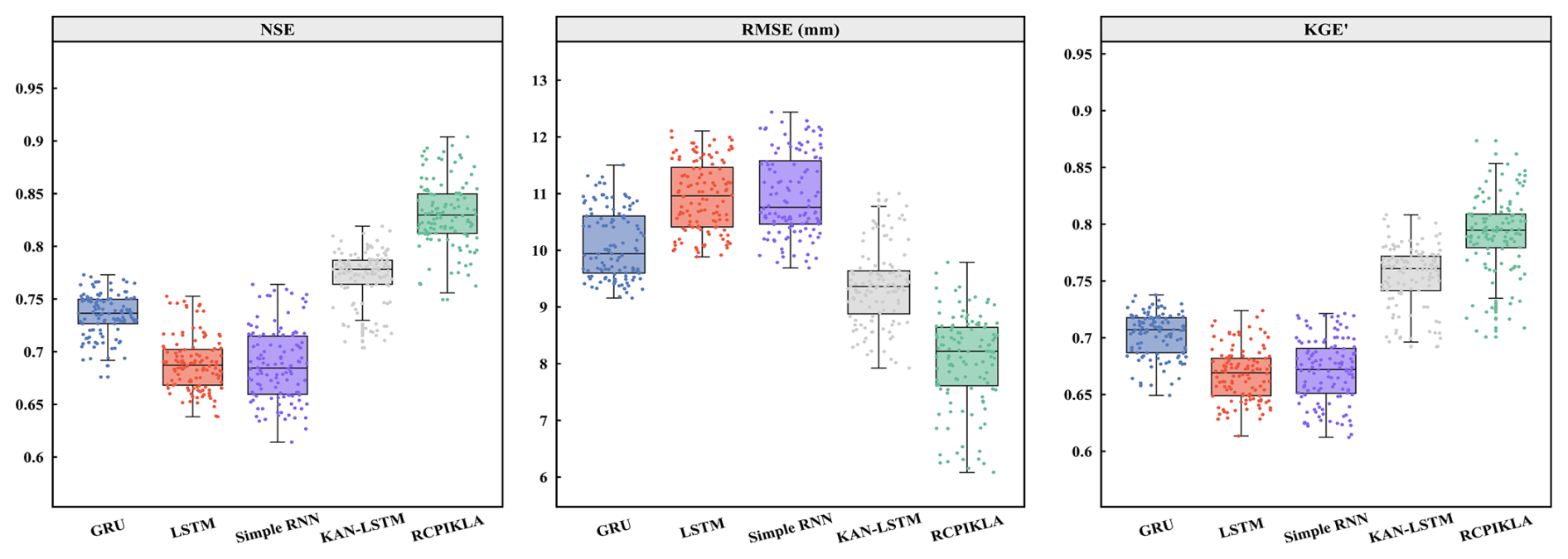
Figure 6 The box plot of NSE (left), RMSE (middle), and KGE^′ (right) values of multiple models of various time steps (1–12 months) for 10 runs.

The evaluation metrics of LSTM, KAN-LSTM (KAN transformation followed by LSTM without attention, physics constraints, or residual compensation), and RCPIKLA are compared and analyzed. Figure 5 presents this comparison alongside other baselines across multiple forecasting horizons (1–12 months), while Fig. 6 shows the distribution of metrics across 10 independent training runs. The comparison between LSTM and KAN-LSTM shows that KAN-based nonlinear feature transformation can produce consistent improvements across all time steps. Averaged across all forecasting horizons, KAN-LSTM achieves NSE of 0.77 (±0.025), RMSE of 9.4 mm (±0.68), and KGE^′ of 0.75 (±0.027), compared to LSTM's NSE of 0.70 (±0.034), RMSE of 10.94 mm (±0.61), and KGE^′ of 0.67 (±0.023). This represents approximately 12 % improvement in NSE attributable specifically to KAN's learnable univariate functions. At the optimal 9-month time step, KAN-LSTM achieves NSE of 0.78 compared to LSTM's 0.70, which demonstrates that KAN provides substantial value for prediction.

4.2 Performance comparison among various deep learning models at different value ranges

As shown in Fig. 5, the optimal performance of the proposed RCPIKLA model is obtained when the time step is 9 months. In addition to temporal comparisons, the predictive performance across different discharge value ranges is further assessed to evaluate how well each model performs under varying flow conditions, from low to high discharge events. The predicted and observed values of the proposed model and baselines when the time step is 9 months are presented in Figs. 7 and 8. The performance metrics reveal substantial differences in model accuracy. The RCPIKLA model demonstrates more robust performance compared to others across all value ranges with the highest NSE coefficient of 0.856, the lowest RMSE of 7.077 mm and the highest KGE^′ of 0.817. This indicates that the proposed hybrid approach, which integrates physics-informed constraints with residual compensation, captures the nonlinear and non-stationary characteristics of the Kolyma River discharge more effectively than other architectures. The GRU model achieves an intermediate performance level (NSE=0.750, RMSE=9.418 mm, ${\text{KGE}}^{\prime }=\mathrm{0.718}$), which outperforms other recurrent neural networks but falls short of KNN based models. Both LSTM and Simple RNN exhibit similar and relatively poorer performance metrics, which demonstrates their limitations in capturing the complex hydrological dynamics of Arctic river systems when used without additional enhancements.

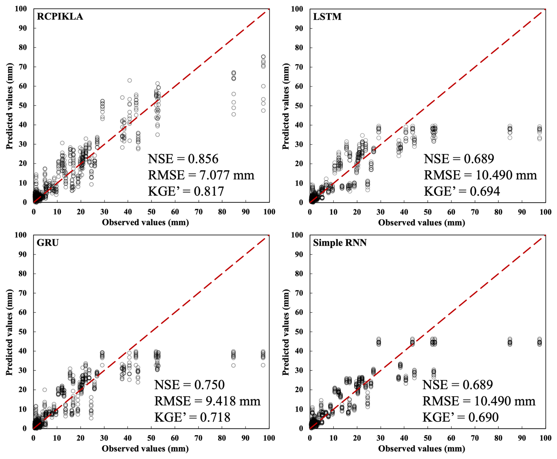
Figure 7 The predicted and observed values of 10 independent runs when the time step is 9 months, including RCPIKLA, LSTM, GRU and Simple RNN models. The red dash line angled at 45° represents the line of perfect agreement between observed and predicted values.

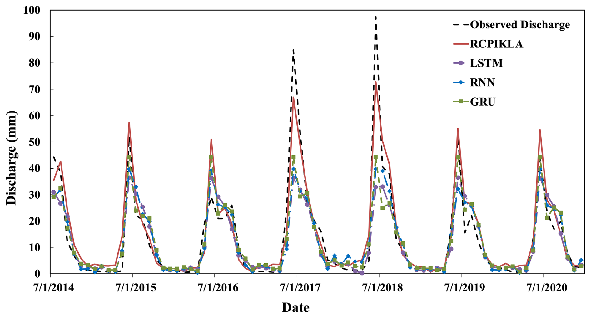
Figure 8 Time series comparison of observed and predicted monthly discharge for the Kolyma River during the test period when the time step is 9 months.

It is worthwhile to note that all models perform reasonably well for low to moderate discharge values (0–30 mm), but significant differences emerge at higher discharge events (>80 mm), which is crucial for flood forecasting. Although the proposed RCPIKLA model maintains better prediction accuracy for these high discharge events, there is room for improvement, which may be attributed to the limited number of high discharge events in the training dataset. This systematic underestimation of peak flows represents a common challenge in data-driven hydrological modeling, particularly for Arctic river systems, where extreme discharge events are relatively rare but carry significant implications for water resource management and hazard mitigation. Kratzert et al. (2019) observed similar patterns in LSTM-based rainfall-runoff modeling across diverse catchments. For Arctic rivers specifically, Gelfan et al. (2017) and Chang et al. (2025) reported that process-based models and machine learning approaches struggle with extreme conditions due to the complex processes and events that are poorly represented in limited observational records. In our study, extreme high discharge events (>80 mm) constitute less than 5 % of the training dataset, creating a class imbalance problem common in hydrological time series (Nearing et al., 2021). The squared error loss function (MSE) used in model training inherently weights all samples equally, which can lead to optimization that favors the more numerous moderate flow events at the expense of rare extremes. Future work could address this limitation through specialized sampling techniques or physics-informed constraints specifically designed to better capture high-magnitude discharge events.

4.3 Interpretability analysis of Kolmogorov–Arnold Networks

Kolmogorov–Arnold Networks can learn interpretable univariate functions that can be visualized and approximated symbolically (Liu et al., 2024). The learned activation functions from the KAN component for each input feature are derived and presented to examine how each hydroclimatic input is transformed prior to temporal aggregation by the LSTM-attention block. While the overall model remains a sequence model, the KAN component offers mechanistic insight into learned input transformations.

Presented in Fig. 9, the learned univariate KAN functions for the primary hydroclimatic predictors and the seasonal encodings are plotted against standardized inputs. The learned mappings show distinct behaviors across variables. Temperature exhibits threshold-dependent behavior and an increasing response for positive standardized values, which are consistent with degree-day snowmelt formulations (Hock, 2003). The minimal response at very low temperatures reflects periods when all precipitation accumulates as snow with no melt contribution to discharge. The strengthening positive trend at high temperatures captures accelerated snowmelt during warmer periods and melt-season activation. The PET function remains relatively constant across most of the range but drops at extremely high PET values. This negative response at high evapotranspiration demand is physically meaningful in permafrost watersheds where shallow active layers and restricted groundwater storage make baseflow highly sensitive to evaporative losses during warm, dry periods. The transition may represent a threshold where evaporative water losses begin to substantially reduce streamflow, consistent with observations of increased Arctic river sensitivity to evapotranspiration under warming (Nijssen et al., 2001). Precipitation shows minimal direct transformation with a nearly flat or slightly negative function. It can be caused by winter precipitation accumulating as snow and contributing to discharge only after spring melt, which creates multi-month lags (Gelfan et al., 2017). The learned functions for the temporal encoding variables (Month_sin and Month_cos) shows how the KAN components represent seasonality. Month_sin exhibits a clear, smoothly varying nonlinear transformation, whereas Month_cos remains comparatively flat. The monotonic tendency in the Month_sin curve suggests an asymmetric seasonal influence. It shows that the model responds differently to the rising and falling portions of the annual cycle, which is consistent with the sharp melt-season transition and the comparatively gradual recession that often follows peak flow. Importantly, because trigonometric encoding provides a continuous cyclical representation of annual timing, the KAN transformation can capture seasonal structure without introducing an artificial discontinuity at the year boundary.

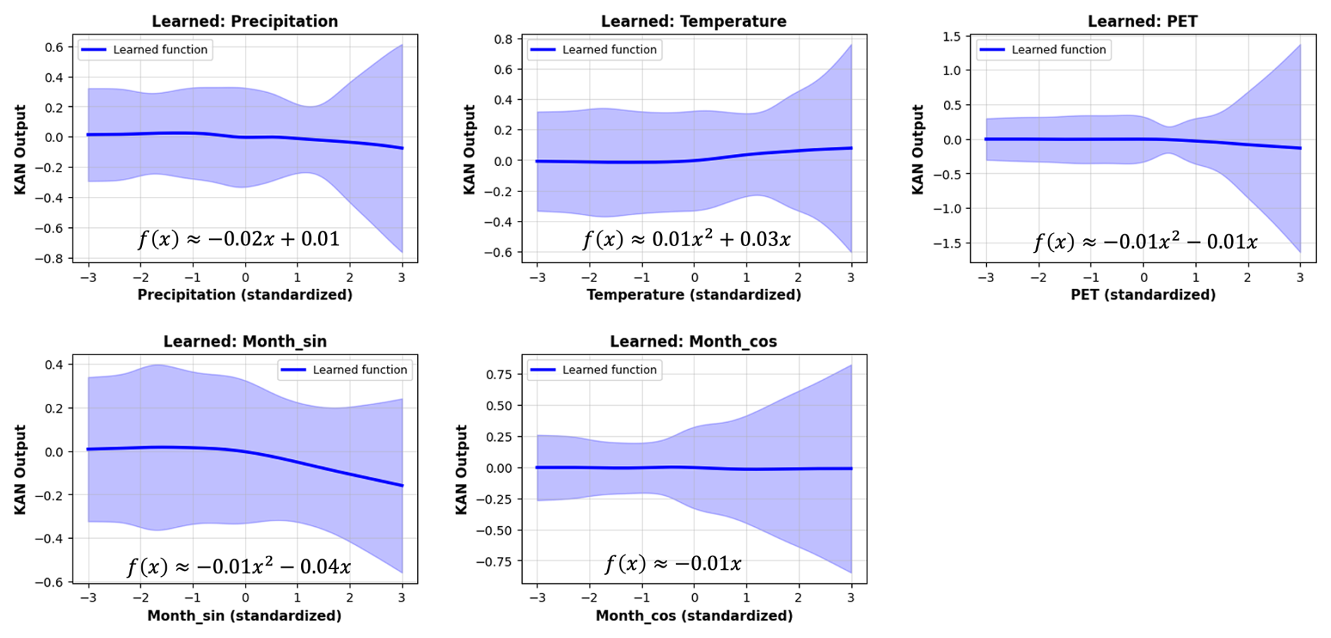
Figure 9 Learned univariate KAN functions for each input variable into the following LSTM component. Each panel shows how a single input feature is transformed before being passed to the LSTM layers. Blue lines represent the mean transformation across all KAN output dimensions, with shaded regions indicating ±1 standard deviation, reflecting transformation variability.

It is worthwhile to note that, as a hybrid architecture, RCPIKLA is primarily interpretable at the KAN stage. As the KAN module represents input–feature mappings through learnable univariate functions, the learned curves and their symbolic approximations provide a transparent description of how each hydroclimatic predictor is transformed before being passed to the sequence model. However, this interpretability does not extend to a fully closed-form, end-to-end explanation of the final discharge prediction: the downstream LSTM block integrates information across multiple antecedent months and mixes transformed features through recurrent dynamics and temporal weighting. Consequently, the KAN-derived functions should be interpreted as input transformations, rather than as a complete mechanistic decomposition of the full temporal prediction process.

4.4 On the role of the physics informed constraints and residual structure

The ablation results comparing RCPIKLA, RCKLA (no physics), and PIKLA (no residual) are presented in Fig. 10. The results reveal that the complete RCPIKLA model achieves mean NSE of 0.827±0.030 (mean ± standard deviation) across 120 evaluations, which represents significant improvements over the PIKLA model without residual compensation (0.790±0.029, p<0.001) and the RCKLA without physics (0.812±0.031, p<0.001). Similarly, RCPIKLA obtains lowest RMSE (8.12±0.75 mm) compared to PIKLA (8.98±0.52 mm, p<0.001) and RCKLA (8.47±0.76 mm, p<0.001). These comparative results highlight two important aspects of the model architecture: (1) The physics-informed constraints contribute to overall model robustness and performance stability. By incorporating physical principles of snowpack accumulation and melt processes through the specialized SnowpackLayer, the model better captures the underlying hydrological dynamics of the Arctic river system. The physics-informed loss function, which mathematically enforces the relationship between melted snow and discharge, helps maintain physical consistency in the predictions. (2) The residual compensation mechanism addresses model inadequacies by learning the systematic errors in the physics-based predictions. This is particularly valuable for handling complex nonlinear processes that are not fully captured by the simplified physical representations. The performance difference between PIKLA and RCPIKLA demonstrates that the residual structure successfully compensates for approximation errors in the physics-informed component. Residuals (Predicted − Observed) are evaluated on the test set across all forecast horizons (1 to 12 time steps), using 10 independent runs per horizon. When pooling all residuals across horizons and runs, RCPIKLA obtains a low residual (0.08 mm, corresponding to +0.57 % of the mean observed discharge), whereas RCKLA exhibits a negative mean residual (−0.31 mm, −2.23 %). These results indicate that the physics-informed constraint does not introduce a systematic bias. Instead, it reduces the slight underprediction tendency of the unconstrained model and yields a more centered residual distribution overall.

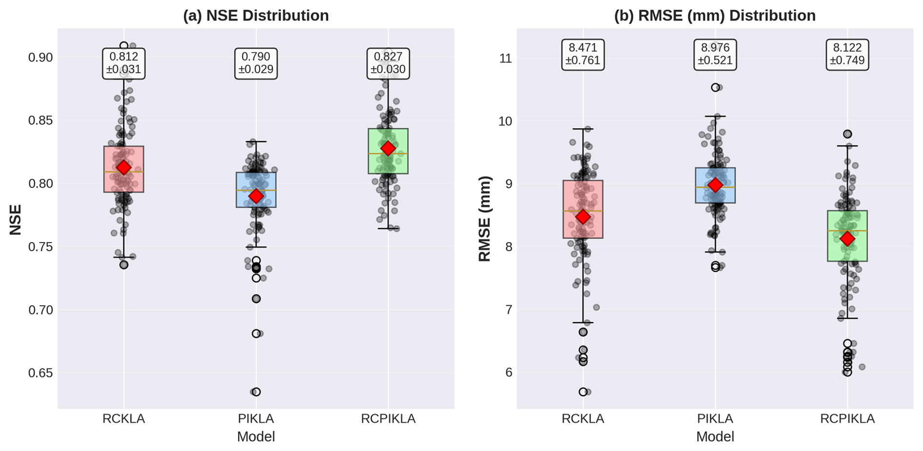
Figure 10 Performance comparison of model variants, including RCPIKLA, PIKLA (no residual) and RCKLA (no physics), across all forecasting horizons (1–12 months) and 10 independent training runs. Box plots show distributions of (a) NSE, and (b) RMSE. Each box aggregates 120 evaluations (12 time steps ×10 runs), with boxes showing median (center line), interquartile range (box edges), and 1.5× IQR whiskers. Individual points represent each evaluation. Red diamonds mark the mean values with numerical annotations (mean ± standard deviation).

In summary, the ablation comparisons isolate individual component contributions: the residual structure (RCPIKLA vs. PIKLA) improves NSE by 0.038 (4.8 % relative improvement), while the physics-informed constraint (RCPIKLA vs. RCKLA) contributes 0.015 NSE improvement (1.8 % relative). Both components provide independent, statistically significant (p<0.001) performance gains, confirming their complementary roles in the hybrid architecture. The synergistic integration of both components yields a new structure that balances data-driven flexibility with physical consistency. This hybrid approach is particularly advantageous in data-limited environments like Arctic rivers, where the physics-informed constraints and the residual compensation help overcome model simplifications and data uncertainty.

4.5 The role of seasonal variations and trigonometric encoding

To assess the contribution of explicit seasonal representation, model variants are evaluated with and without trigonometric encoding (TE) of monthly seasonality. The comparative analysis is plotted in Fig. 11, which reveals substantial performance differences across NSE, RMSE, and KGE^′ metrics. The results are aggregated across all time step, with each time step evaluated using 10 independent runs. The box plot of three evaluation metrics indicates that trigonometric encoding substantially improves performance across all model architectures. The proposed RCPIKLA model maintains the highest median NSE (approximately 0.83) with trigonometric encoding, while the removal of TE (denoted by “-no TE”) leads to degraded performance (median NSE around 0.80) and wider value ranges. This pattern is consistent across all architectures, with GRU, LSTM, and Simple RNN models all exhibiting substantial performance degradation when seasonal encoding is removed. The widths of the box plots, representing interquartile ranges, also decrease substantially with TE, indicating greater consistency and reduced variability across model runs. Similar improvements are observed in GRU, LSTM, and Simple RNN models. In particular, the LSTM and Simple RNN models without trigonometric encoding show greater instability, with some runs achieving NSE values below 0.5, which shows severely compromised predictive capability. Regarding RMSE, the incorporation of TE effectively reduces median errors and decreases variability, particularly for RCPIKLA, where RMSE values exhibit the narrowest range. Outliers observed in models without trigonometric encoding suggest that omitting seasonal encodings can lead to occasional severe prediction errors, likely caused by the model's inability to account effectively for seasonal patterns. The KGE^′ metric corroborates these findings, with RCPIKLA achieving a median KGE^′ of 0.781 with TE and 0.750 without TE (4.1 % improvement). Baseline models show improvements of 2.5 %–4.7 % when adding TE, with LSTM and Simple RNN exhibiting the largest gains (0.638 to 0.668 and 0.641 to 0.671, respectively). This indicates that while trigonometric encoding provides universal benefits across all architectures, the combination of RCPIKLA's physics-informed components with TE yields synergistic improvements, achieving the best overall performance across all three metrics.

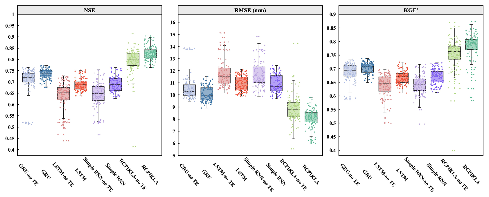
Figure 11 The comparison of models with and without trigonometric encoding for seasonal variations as inputs.

Overall, the performance improvements from trigonometric seasonal encoding observed across all model architectures highlight the importance of explicit temporal feature engineering in hydrological applications. This finding is consistent with recent deep learning studies in environmental and hydrological modeling. For example, Pölz et al. (2024) demonstrated that providing deep learning models with explicit time-aware features such as cyclical time features improved discharge prediction compared to expecting the model to learn seasonal patterns solely from data. Snieder and Khan (2025) also supported cyclical encoding from a methodological perspective, as encoding time with sine–cosine terms provides a continuous, cyclic representation of annual timing. This avoids the artificial discontinuity at the year boundary, which can otherwise introduce spurious jumps and make seasonal relationships harder for data-driven models to learn.

The results showing that baseline models (LSTM, GRU) gain 4.7 % performance from TE, while the physics-informed RCPIKLA gains 4.1 %, suggests that different model components capture seasonal information through complementary mechanisms. The physics-informed snowpack layer already provides implicit seasonal awareness through temperature-dependent snow accumulation and melt, which may explain why RCPIKLA benefits slightly less from explicit TE. Without explicit encoding of this cyclical pattern, models struggle to establish accurate temporal context for the meteorological inputs, resulting in compromised predictive accuracy.

5 Conclusion

In this study, a novel hybrid model integrating physics-informed constraints with advanced deep learning architectures is proposed to improve discharge prediction accuracy in permafrost-dominated Arctic rivers. The proposed RCPIKLA model obtains robust and accurate prediction performance on the Kolyma River, outperforming conventional deep learning approaches across all forecasting horizons from 1 to 12 months. The key findings are summarized as follows:

1. The predictive performance of the newly proposed model and baseline models are plotted and evaluated across a range of time steps, from 1 to 12 months. As illustrated in Fig. 5, the newly proposed model consistently overperforms other baselines at all time steps and produces robust predictive performance. It obtains the highest NSE values ranging from 0.81 to 0.86, the lowest RMSE values between 7.1 to 8.5 mm and the highest KGE^′ values between 0.74 to 0.82. The hybrid model achieves optimal performance at 9-month input sequences, which suggests that the permafrost-covered Arctic river discharge exhibits multi-seasonal temporal dependencies on preceding hydrometeorological conditions, such as snow accumulation and melting processes and active layer storage dynamics.

2. The predictive performance across different discharge value ranges is further assessed to understand how well each model captures the full spectrum of hydrological variability. All models perform reasonably well for low to moderate discharge values (0–30 mm), but more obvious differences emerge at moderate and high discharge events. Although the proposed RCPIKLA model maintains improved prediction accuracy, challenges remain in accurately predicting extreme high discharge events, with all models showing a tendency to underestimate peak flows. This limitation may be partially attributed to the relatively sparse representation of high discharge events in the dataset, which constrains the model's ability to generalize under extreme hydrological scenarios.

3. Both physics-informed constraints and residual compensation contribute distinctly to model performance. The physics-informed component, which incorporates snowpack accumulation and melt processes, provides the proposed model with basic domain knowledge that helps overcome data limitations in the permafrost-dominated Kolyma River basin. The residual compensation mechanism examines systematic errors in the physics-based predictions and helps capture complex nonlinear processes that are not fully represented.

4. By transforming month values into sine and cosine components that preserve the cyclical nature of seasonal patterns, the incorporation of trigonometric seasonal encoding can improve the predictive performance. This approach enhances prediction accuracy across all architectures, with improvements of 4 %–6 % in performance metrics, highlighting the importance of representing the pronounced seasonal dynamics of Arctic rivers characterized by frozen winter conditions, spring snowmelt peaks, and moderate summer flows.

While the RCPIKLA model demonstrates robust performance for the Kolyma River prediction under historical and current hydroclimatic conditions, several limitations should be acknowledged. As a data-driven model trained on historical observations, the model's performance may degrade if climate change induces fundamental shifts in watershed behavior that extend beyond the range of training conditions. Such regime changes may include but are not limited to scenarios like transitions from continuous to discontinuous permafrost, and significantly altered seasonal patterns. Under such scenarios, the model would need to extrapolate beyond its training data range, which remains a challenge for data-driven approaches. Future applications under changing climate conditions should include regular model retraining and validation as new observations become available.