Hydrogeological characterization of alpine karst using the transient analysis of flow and transport

Karst springs in alpine catchments are important for maintaining groundwater-dependent ecosystems in fragile environments and for sustaining baseflow in mountain rivers. Despite its importance, rugged and remote terrains pose major challenges in hydrogeological studies of alpine karst. This study developed a practical approach for characterizing an alpine karst system in the Canadian Rocky Mountains that had no previous information aside from the location of the spring outlet. Using geological maps, satellite images, simple water balance, water sampling and analysis, and dye tracer tests, it was possible to estimate the extent of the spring catchment and infer the hydrogeological characteristics of the karst system. Of particular importance was the information obtained from the fluctuations of spring discharge and electrical conductivity in response to diurnal snowmelt cycles. Synthesis of the diverse data set indicates that the karst system has a large volume of groundwater stored in the fractured rock matrix that buffers the interannual variability of precipitation and sustains steady baseflow throughout the year. The karst system consists of fractured rock matrix, saturated conduits acting like pipes, unsaturated conduits acting like open channels, and many pools delaying the propagation of transport and hydraulic signals through the conduit network. The approach developed in this study will be applicable to other alpine karst systems in snow-dominated catchments in rugged and remote terrains.

1 Introduction

Karst aquifers cover 15 % of the Earth's ice-free continental surface (Goldscheider et al., 2020) and supply freshwater to 9 % of the global population (Stevanović, 2019). Karst aquifers in alpine terrains have distinct hydrogeological characteristics, whereby high topographic gradients and lack of vegetative cover enhance groundwater circulation, and result in rapid recharge and highly seasonal flow (Werner, 1979). Springs discharging from karst aquifers sustain perennial flow in alpine streams and maintain stable water temperature, thereby providing an important ecological niche in fragile environments (Goldscheider, 2019; Stevanović et al., 2024, p. 130). Despite their importance, research on alpine karst aquifers is limited due to difficulties of conducting hydrogeological field work in remote and rugged terrains. Previous studies have been primarily conducted in the European Alps (e.g., Frank et al., 2019; Goldscheider, 2005; Gremaud et al., 2009; Krainer et al., 2021; Lauber and Goldscheider, 2014; Lucianetti et al., 2016; Schäffer et al., 2020). Most hydrogeological studies of alpine karst in North America were conducted in the Canadian Rockies from the 1970s to 1990s (e.g., Drake and Ford, 1976; Ford, 1971a, b, 1983a, b; Smart, 1983; Smart and Ford, 1986; Worthington, 1991), with only a few recent studies conducted in the United States (Lachmar et al., 2021; Tobin and Schwartz, 2020).

While the lack of vehicle access in remote alpine terrains poses major challenges for conventional hydrogeological field work, the unique alpine settings offer potential advantages that are not available in lowlands, for example, distinct diel cycles of snowmelt. Snow accumulation and melt have a strong hydrological influence in mid-latitude alpine regions, where the terrain is covered by snow for more than half of a year and rapid snowmelt over two to three months dominates the water input. This results in a binary mode of spring discharge consisting of a relatively short and intense freshet followed by a long period of baseflow. Snowmelt and glacier melt have a pronounced diel cycle influencing the water input, resulting in strong diel fluctuations in discharge and water chemistry of alpine streams (e.g., Muir et al., 2011). The strong seasonal variability and diel fluctuations of water input may be transmitted from recharge areas to the spring through the complex flow pathways consisting of fractured rock matrix and conduits (e.g., Jourde and Wang, 2023; Worthington et al., 2016). The modulation of input “signals” along the flow pathways may be interpreted using standard signal-analysis methods, offering valuable insights into the hydrogeological behaviour of the karst system. The signal-analysis approach (e.g., cross-correlation analysis) has been commonly used in karst hydrogeology (Fiorillo and Doglioni, 2010; Howell et al., 2019; Jódar et al., 2020; Kovačič, 2010; Mangin, 1984; Rahnemaei et al., 2005), however, their application to diel signals in snowmelt-dominated systems has not been widely explored.

In this study, a previously unstudied alpine karst spring in the Canadian Rockies is used to develop a practical approach for the hydrogeological characterization of alpine karst systems in remote, rugged terrains. The research objectives are: (1) delineate the extent of the spring catchment, (2) evaluate the relative volume of groundwater stored over winter with respect to seasonal discharge during the high flow period, (3) characterize the flow and transport dynamics of the karst system, and (4) develop a set of tools for hydrogeological investigation of similar alpine karst systems. The novelty of this study is in the combined application of multiple approaches encompassing hydrological, chemical, isotopic, and mathematical tools to improve the process understanding of a high alpine karst system. The insights and tools developed in this study will be useful for characterizing similar mountain karst systems in snow-dominated regions and their responses to changes in environmental conditions.

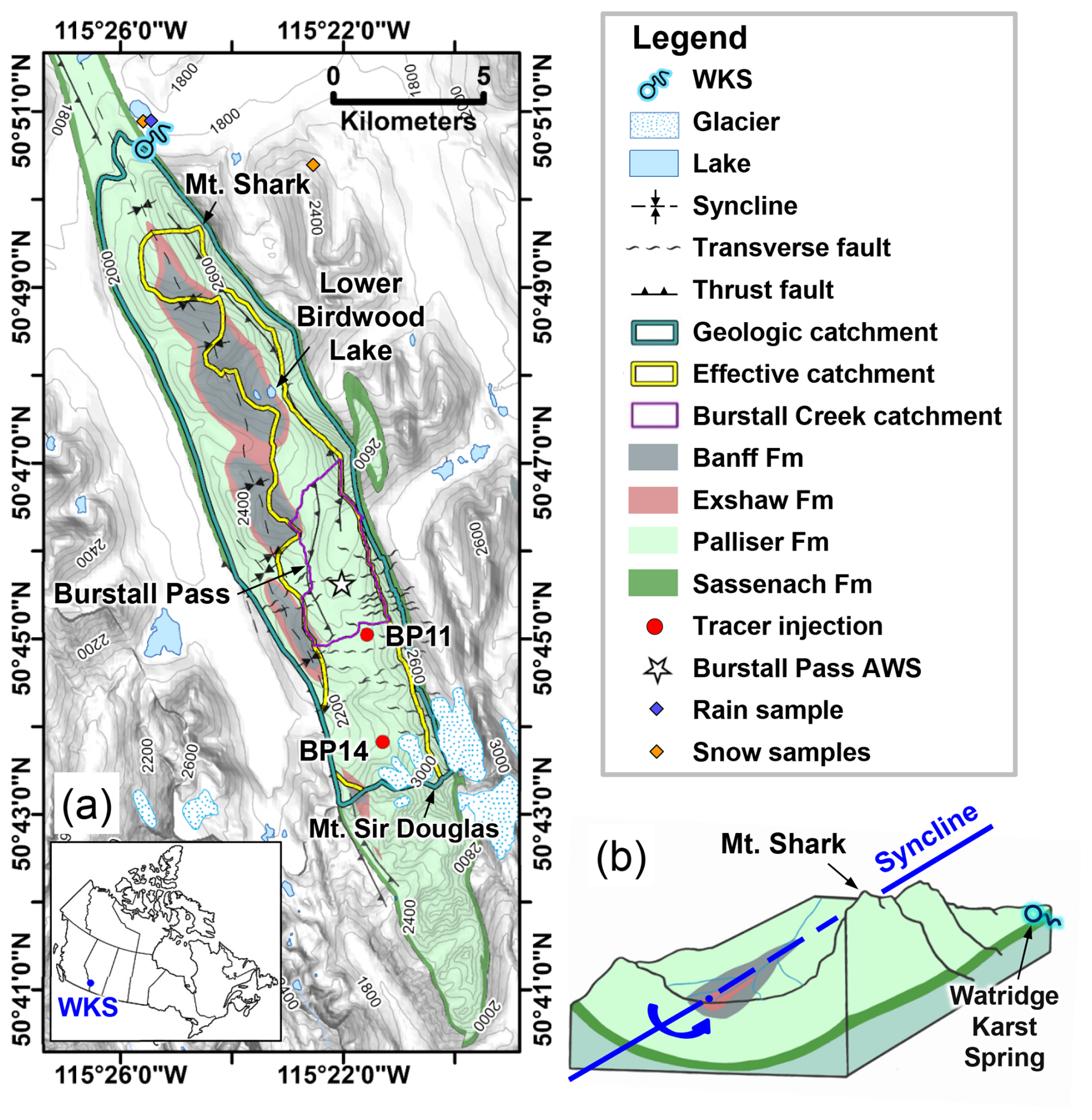
Figure 1 (a) Map of the northern Spray Mountains showing relevant geological formations within a regional plunging syncline, trending NNW-SSE. Elevation contour lines (100 m interval) are drawn to indicate topography. The map also shows the extent of hydrological features and tracer release points. The insert shows the location of the study site within Canada. (b) A conceptual block diagram showing the structure of the northwest-plunging syncline with respect to the summit of Mount Shark, and the Watridge Karst Spring (WKS). The colours correspond to the geological formations in the legend.

2 Study Site

This study investigated the hydrogeology of the Watridge Karst Spring (WKS), located on the northern tip of Mount Shark (50°50^′36^′′ N, 115°25^′38^′′ W) at an elevation of 1870 m (Fig. 1). The adjoining Spray Mountains are approximately 30 km long and consist of steep-sided mountain ridges and glaciated alpine cirques. Treeline occurs at approximately 2300 m, above which the ground is mostly barren as the growing season is too short for tree growth (Downing and Pettapiece, 2006). The mountain ridges continue south to Mount Sir Douglas (3406 m). The spring outlet is situated on a shady north-facing slope, accessible only by foot on a 5 km hiking trail. The spring provides year-round humidity to the surrounding forest, creating a unique habitat for hygrophytic shrubs and mosses (Toop and de la Cruz, 2002). Twenty-five species of mosses, eight hepatics, and seven lichens were identified by WCBLIG (2015), highlighting the uniqueness of the spring's microclimate providing moist habitats. The relatively large entrance and high volume of water discharging from the spring holds promise for an extensive cave network (Lilley and Crisp, 2022).

Although the source of spring water had not been identified prior to the current study, the WKS is expected to be recharged by snowmelt and rain over the rugged terrain of northern Spray Mountain range. The high-elevation snowpack can persist until August, and the upper sections of glaciers are perennially covered in snow. The mean annual air temperature at the Burstall Pass automatic weather station (AWS) (Fig. 1) was −0.5 °C during 2014–2023 (CRHO, 2025), while the mean annual precipitation was 1183 mm. During 2017–2023, mean annual discharge of the WKS was 1.9×10⁷ m³ yr⁻¹ (or 600 L s⁻¹), varying between 16 and 3200 L s⁻¹, with the median value of 300 L s⁻¹.

The Front Ranges of the Rocky Mountains is dominated by major thrust faults, and both broad and steeply dipping folds of Paleozoic and Mesozoic strata (McMechan, 2012). The bedrock of Spray Mountains is composed of the massive Devonian Palliser Fm., a major cliff-forming unit consisting primarily of limestone and dolomitic limestone (Holter, 1976; de Wit and McLaren, 1950). A stratal thickness of approximately 280 m is typical in the Front Ranges (de Wit and McLaren, 1950). The Palliser Fm. is an established karst unit in the Front Ranges (Smart, 1988; Yonge and Lowe, 2017) and is known to have groundwater velocities exceeding 0.1 m s⁻¹ (Worthington, 1991). Anhydrite has been described as an important constituent of the uppermost and lowermost sections of the Palliser Fm. (Andrichuk, 1960; Clark, 1949; Fox, 1951; Govett, 1961; MacNeil, 1943; Nightingale and Mayer, 2012). The WKS occurs at the base of the Palliser Fm., at the inferred contact between the Palliser Fm. and the underlying Sassenach Fm. (McMechan, 2012; Lilley, 2023), which is considered an aquitard (Worthington, 1991). The Mississippian Exshaw and Banff Fms. overly the Palliser Fm. These units are composed of black pyritiferous shales, interbedded mudstones, limestones, siltstones, and sandstones; and they do not behave as karst aquifers (Beales, 1956; McMechan, 2012).

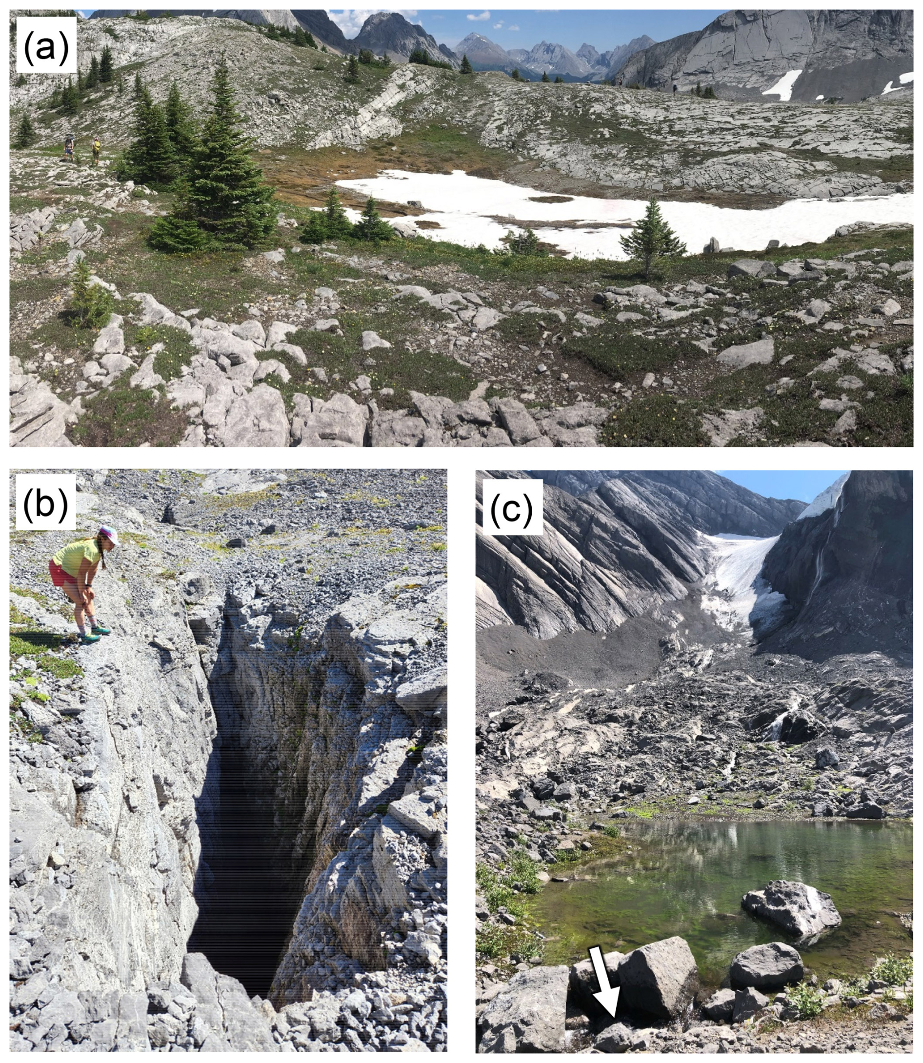
Figure 2 (a) Limestone pavement in foreground and a depression serving as a natural infiltration basin in the Burstall plateau near BP11 (9 July 2021). (b) Tracer injection location (BP11) in dry condition (31 August 2022). (c) Pond draining into a swallet (arrow), which served as a tracer injection location (BP14); looking south towards Mount Sir Douglas displaying steeply dipping synclinal bedding of the Palliser Fm. (11 August 2021).

In the southern direction along the Spray Mountains, the continuous extension of the Palliser Fm. above the elevation of the WKS is a potential recharge area. Surface karst geomorphology, sinking streams, depressions serving as infiltration basins (Fig. 2a) are prevalent in the plateau area south of Burstall Pass AWS and towards Mount Sir Douglas. Several shafts, dolines, and limestone pavements were observed on the plateau. Some of these karst features appeared to be located along the synclinal axis or transverse faults. Snowmelt has been observed cascading into vertical shafts, and the influence of daily snowmelt is noticeable in diel fluctuations of discharge and electrical conductivity (EC) of the WKS (see below). Lilley (2023) observed a low amount of total annual runoff (23 mm) in Burstall Creek draining a small (4.5 km²) watershed located within the plateau area (Fig. 1a), indicating that much of runoff occurred as subsurface drainage to the karst system. Smaller but considerable amount of recharge is expected in other parts of the catchment devoid of vegetation. For example, Lilley (2023) estimated a recharge rate of 10 mm d⁻¹ from the Lower Birdwood Lake (Fig. 1a) in a topographically closed basin during a 20 d period in September 2020, indicating the ability of the weathered near-surface zone of Banff Fm. to allow local infiltration of snowmelt water.

3 Methods

3.1 Stream discharge and physical parameters

The WKS was continuously monitored from 2017 to 2023. Water level was recorded at 30 min intervals using a non-vented pressure transducer (Solinst, Levelogger) in a stilling well and compensated for barometric pressure measured using a separate transducer (Solinst Barologger) located approximately 5 m from the spring outlet. Stream discharge was manually measured using the velocity-area method (Dingman, 2002, p. 609) and a horizontal-axis current meter (Global Water, FP111) on a regular basis. Sources of uncertainty in the stream hydrographs are manual discharge measurement errors, curve fitting errors, and the accuracy of the recorder. Hood et al. (2006) found that the coefficient of variability for an alpine stream discharge measured by the same method was up to 9 %. Regular discharge measurements across the full spectrum of flow conditions minimized the uncertainty for the WKS hydrograph. A root-mean-squared error (RMSE) of 85 L s⁻¹ was obtained for the WKS rating curve from 43 measurements of stream discharge, yielding an uncertainty of 13 %. Assuming that individual error components are independent and randomly distributed, the total uncertainty of the WKS hydrograph is ∼16 % (Rosenberry and Hayashi, 2013, p. 171).

Data loggers were used to record EC and water temperature and were calibrated using manual measurements. EC was measured using a handheld meter (VWR, 21800-012) and compensated to 25 °C (Hayashi, 2004). EC was recorded at 30 min intervals using a conductivity sensor (Onset HOBO, U24-001) at an accuracy of ±5 µS cm⁻¹ and was automatically compensated to 25 °C. Manual EC measurements served to correct for instrumental drift of the logger. Water temperature was recorded by a platinum resistance temperature detector built into a pressure transducer (Solinst, Levelogger) at 30 min intervals, with an accuracy of ±0.05 °C. Temperature readings were checked against manual measurements using a handheld thermocouple thermometer (Omega Engineering, HH-25TC).

3.2 Water sampling and analysis

A total of 125 spring water samples were collected and analyzed for major ion chemistry. All samples were filtered with 0.45 µm membrane filters and stored in a refrigerator in pre-rinsed high-density polyethylene bottles prior to analysis. During May–October of 2020 and 2021, samples were collected every 1 to 4 d by an autosampler (Teledyne ISCO, 6712) at the WKS. To minimize evaporation, each sample bottle contained a ping-pong ball and was filled to the narrow portion of the bottleneck so that the ball covered most of the water surface. Water samples were also collected manually at the time of discharge and EC measurements (see above) and pH was measured using a handheld meter (Barnant, 559-3800).

Rainwater was collected in a small shrubby wetland sheltered from strong winds, near the spring (Fig. 1a) using a ball-in-funnel type collector (Prechsl et al., 2014) to prevent evaporation and block debris. Aggregated rainwater was retrieved once every few weeks from the sampler. Depth-integrated snow samples were collected from two locations (Fig. 1a) using a snow sampler with a 39.1 cm² cutting area (Farnes et al., 1982) and melted in the laboratory to yield an integrated sample.

Major cations and anions were measured using ion chromatography (Metrohm 930 Compact IC Flex) with an analytical precision of 0.2 % to 0.8 %. Alkalinity was determined by titration with an estimated uncertainty of 3 %. Samples with a charge balance error >5 % were rejected. The ${}^{\mathrm{2}}\mathrm{H}{/}^{\mathrm{1}}\mathrm{H}$ and ${}^{\mathrm{18}}\mathrm{O}{/}^{\mathrm{16}}\mathrm{O}$ isotopic ratios of water were measured by cavity ring-down spectroscopy (Los Gatos Research, DLT-100) and reported as δ-values relative to Vienna Standard Mean Ocean Water (V-SMOW) with an analytical uncertainty of 0.1 ‰ for δ¹⁸O and 1 ‰ for δ²H. Tritium in water was analyzed at the University of Waterloo Environmental Isotope Laboratory using liquid scintillation counting after 15-times enrichment by electrolysis, providing a detection limit of 0.8 tritium units (TU). For those water samples with manual pH measurements, saturation indices of carbonate and sulfate minerals were calculated using the geochemical speciation program PHREEQC (Parkhurst and Appelo, 2013).

Select samples from the spring were analyzed for stable isotope ratios of dissolved SO₄ (${}^{\mathrm{34}}\mathrm{S}{/}^{\mathrm{32}}\mathrm{S}$ and ${}^{\mathrm{18}}\mathrm{O}{/}^{\mathrm{16}}\mathrm{O}$). The samples were processed following the standard SO₄ extraction technique (Lilley, 2023) and the isotope ratios of dissolved SO₄ were analyzed using continuous flow-isotope ratio mass spectrometry. The isotope ratios are reported as δ-values relative to Vienna Canyon Diablo Troilite for ³⁴S and V-SMOW for ¹⁸O with an analytical uncertainty of 0.3 ‰ for δ³⁴S and 1 ‰ for δ¹⁸O.

Water samples for dissolved ²²²Rn were collected from the spring in two 250 mL glass bottles by submerging them underwater in the spring and the cap was fastened while underwater to prevent contamination from atmospheric gases. The ²²²Rn activity was measured in the laboratory with a portable radon detector (Durridge, RAD7). A closed-loop aeration device (Durridge, RAD H2O) was used, whereby air recirculated through the water sample to continuously extract radon until a state of equilibrium is achieved. The ²²²Rn activity in water was calculated by multiplying the air loop concentration by a fixed conversion coefficient dependent on the sample size using CAPTURE software (Durridge Company Inc., 2014) and corrected for the decay during storage.

3.3 Meteorological data

Air temperature and precipitation data recorded at the Burstall Pass AWS (Fig. 1) were used in this study. The AWS is in an open canopy forest just below treeline at an elevation of 2260 m (CRHO, 2025), and the instruments include an air temperature/relative humidity sensor (FTS, SDI-THS-LB) and a weighing precipitation gauge (OTT, Pluvio²). Hypsometric analysis of the effective catchment of the WKS (see Sect. 4.2 for definition) indicates that ∼70 % of the catchment is contained within an elevation range of 2100–2500 m and the median elevation of the catchment is 2420 m. Therefore, the AWS represents average temperature and precipitation of the catchment reasonably well. Precipitation data were supplemented by the data from nearby weather stations (ACIS, 2025; CRHO, 2025) to fill short gaps. Consistency across data sources was ensured through double mass curve analysis, which also helped detect any discrepancies across precipitation records. In cases of potentially erroneous precipitation data, historical radar data extracted from ECCC (2025) was consulted to verify the occurrence, timing, and extent of a precipitation event. Due to these gap-filling measures, it was not practical to apply the correction for wind-induced undercatch of solid precipitation for the entire data set. Therefore, the precipitation data were used without correction. The magnitude of undercatch is estimated to be ∼5 % of annual precipitation (Smith et al., 2022, Fig. 6b).

3.4 Fluorometry and dye tracing

A fluorescent dye tracer, uranine (colour index: Acid Yellow 73, CAS No. 518-47-8) was used in this study. Uranine has a low sorption tendency, low detection limit, low toxicity, and relatively conservative behaviour (Goldscheider et al., 2008). A fluorometer (Turner Designs, Cyclops 7F) was installed at the WKS, equipped with a shade cap, fastened to a steel-bar post that was hammered into the stream bed, and connected to a datalogger (Campbell Scientific, CR1000).

Three tracer injections were performed at two locations: BP11 and BP14 (Fig. 1). Due to long hikes required to reach the tracer injection locations, the dye was carried in powder form and dissolved in surface water from the local source. The BP11 site is a large shaft (Fig. 2b) and is one example of many surface karst features on the Burstall Pass plateau. The entrance to BP11 is located at the base of a large (>8000 m²) depression that holds snow until middle or late July. This snow drains into the shaft, making it a suitable location for tracer injection as the dye could be flushed by the melting snow. The BP14 site is a swallet that drains the glacial meltwater from the western glacier of Mount Sir Douglas (Fig. 2c).

Tracer velocities and mean travel times were calculated from the resultant breakthrough curves. The mean travel time (t_m, s) is the time required for the centre of mass of the dye cloud to traverse the entire length of the aquifer system and defined by (USEPA, 2002):

$$\begin{array}{}\text{(1)}& t_{\mathrm{m}}=\underset{\mathrm{0}}{\overset{\mathrm{\infty }}{\int }}tU\left(t\right)Q\left(t\right)\mathrm{d}t/\underset{\mathrm{0}}{\overset{\mathrm{\infty }}{\int }}U\left(t\right)Q\left(t\right)\mathrm{d}t\end{array}$$

where t (s) is the time elapsed since injection, U and Q are uranine concentration (kg m⁻³) and spring discharge (m³ s⁻¹) at time t, respectively.

The mean tracer velocity (v_m, m s⁻¹) is given by (Mull et al., 1988; USEPA, 2002):

$$\begin{array}{}\text{(2)}& v_{\mathrm{m}}=l_{\mathrm{s}}/t_{\mathrm{m}}\end{array}$$

where l_s (m) is an estimated length of the tracer travel path. A sinuosity factor (S_F) is used to estimate l_s from the linear distance l_min (m) between the injection and sampling points, reflecting a more realistic conduit path length (Field and Nash, 1997; Worthington, 1991, p. 138):

$$\begin{array}{}\text{(3)}& l_{\mathrm{s}}=S_{\mathrm{F}}{l}_{\min }\end{array}$$

where typical values of S_F for solutional conduits range from 1.3 to 1.5 (USEPA, 2002). Worthington (1991) reported an average S_F of 1.56 for 96 complete flow paths in karst aquifers from around the world. Among these, the Castleguard karst in the Front Ranges (Smart, 1983), 190 km northwest of the WKS had an S_F of 1.21. Based on these published figures, a range of S_F from 1.2 to 1.6 was used in this study to estimate lower and upper bounds of tracer velocities.

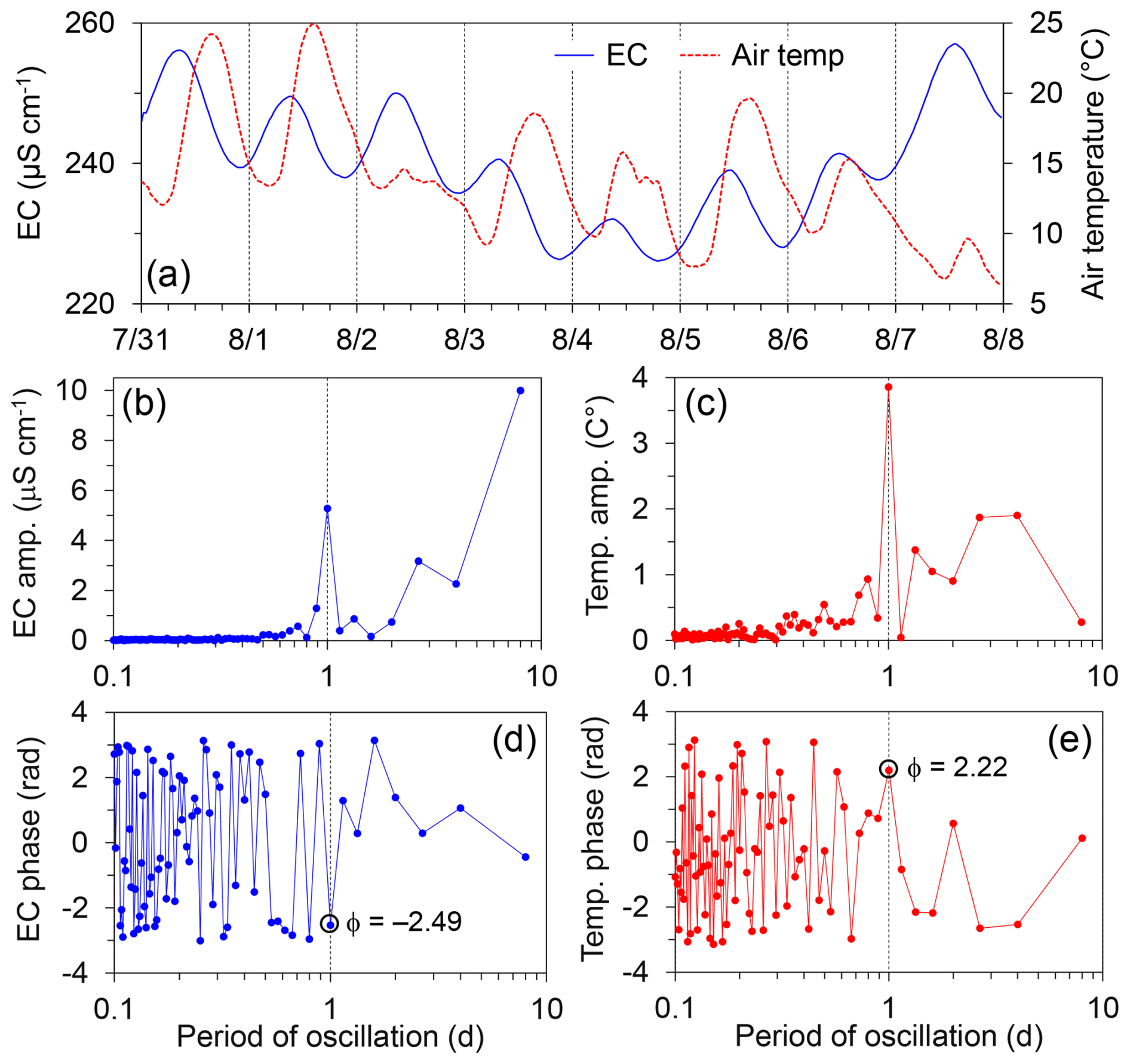
Figure 3 An example of fast Fourier transform (FFT) results from 31 July–8 August 2021. (a) The original time series of electrical conductivity (EC) and air temperature. A 4 h moving average filter was applied to smooth the data for the plotting purpose. (b) Amplitudes of EC signal in the frequency domain plotted against the period of oscillation. (c) Amplitudes of air temperature in the frequency domain. (d) Phase angles (φ) of EC signals. (e) Phase angles of air temperature. The phase angles of the diel component are indicated in the graphs.

3.5 Analysis of diel fluctuations of discharge and EC

Spring discharge and EC had diel fluctuations in response to snowmelt and glacier melt as demonstrated in an example of EC fluctuations (Fig. 3a). To examine the effects of snowmelt on spring discharge and chemistry, air temperature was used as a proxy for the magnitude of energy inputs for snowmelt (Vigna and Banzato, 2015). More specifically, it was assumed that, on a given day, the timing of maximum snowmelt coincided with maximum air temperature, meaning that the daily peak of total energy input by net radiation and turbulent heat transfer coincided with the peak air temperature and that the transit time of snowmelt through the snowpack was of secondary importance. The time lag of diel fluctuations between air temperature and discharge defined the hydraulic response time, and air temperature and EC the transport response time, analogous to pulse-through time and flow-through time defined by Ford and Williams (2007, p. 125).

The Fourier transform was used to determine the phase hours (i.e. timing of peaks and troughs) of diel fluctuations, and the phase hours of EC and discharge were compared against the phase hour of air temperature to determine the phase lag. The fast Fourier transform (FFT) algorithm of Virtanen et al. (2020) was used to compute the discrete Fourier transform:

$$\begin{array}{}\text{(4)}& F_k={\sum }_{n=\mathrm{0}}^{N-\mathrm{1}}{f}_n\exp (-i\mathrm{2}\mathit{\pi }kn/N)\end{array}$$

where F_k is the kth element of the transformed sequence in the frequency domain, f_n is the nth element (i.e. data point) of the original time series, N is the total number of data points, k is the index of the frequency component in the frequency domain, ranging from 0 to N−1, and n is the index of the time-domain sequence.

The output of the FFT is an array of complex numbers F_k, which contains information on the timing (i.e. phase) and strength (i.e. amplitude) of each frequency in the original function. The phase and magnitude of diel signals were computed throughout the snowmelt season of 2020 and 2021 by (1) extracting an 8 d period from a given dataset (e.g., Fig. 3a), (2) applying the FFT, and (3) shifting the period forward by 2 d and repeating the computation. Each 8 d data period was linearly detrended to allow for the periodic extension of the time series data.

Of particular interest is the diel component with an oscillation period (T_p) of 24 h, which has a corresponding angular frequency ($=\mathrm{2}\mathit{\pi }/T_{\mathrm{p}}$) of 0.2618 rad h⁻¹. The amplitudes of F_k plotted against T_p (Fig. 3b and c) indicate the relative strength of oscillation in discharge (in L s⁻¹) or EC (µS cm⁻¹) contained in each component. For each 8 d period, the phase angle (φ, rad) of frequency components were computed from F_k (Fig. 3d and e), and φ of the diel component was converted from radians to hours by multiplying φ by $T_{\mathrm{p}}/\mathrm{2}\mathit{\pi }$. This provided a “phase hour” as a time relative to 00:00 LT (midnight). For example, a phase hour of +8.5 signified a signal maximum that occurred 8.5 h prior to midnight (i.e., 15:30) in Mountain Daylight Time (Coordinated Universal Time minus 6 h). Conversely, a phase hour of −9.5 signified a maximum that occurred 9.5 h after midnight (i.e., 09:30). Finally, the difference between the phase of air temperature and EC/discharge was determined. This method provides a reliable means of determining phase lag, but with the inherent problem that results may represent any multiples of 24 h. To determine the actual time lag, visual inspection of EC/discharge to clearly defined events, such as a sudden stoppage or weakening of snowmelt due to cold weather (Fig. 4), was used to calibrate the phase hours.

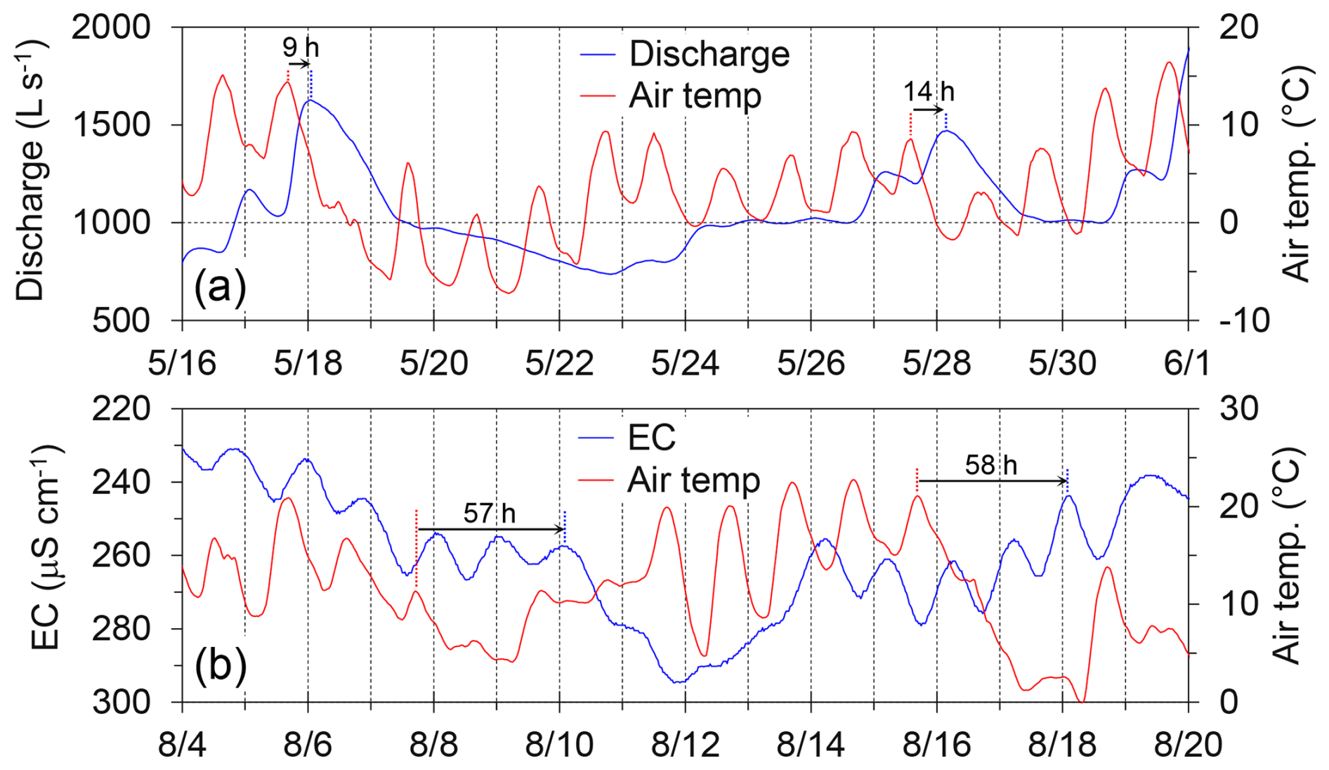
Figure 4 (a) Spring discharge and air temperature during 16–31 May 2021, indicating time lags between air-temperature and discharge peaks corresponding to snowmelt-stoppage events. Vertical lines indicate the midnight of each day. (b) Electrical conductivity (EC) and air temperature during 4–19 August 2021, indicating time lags between air-temperature peaks and EC troughs corresponding to weakening of snowmelt flux. Note that a reverse scale is used for EC.

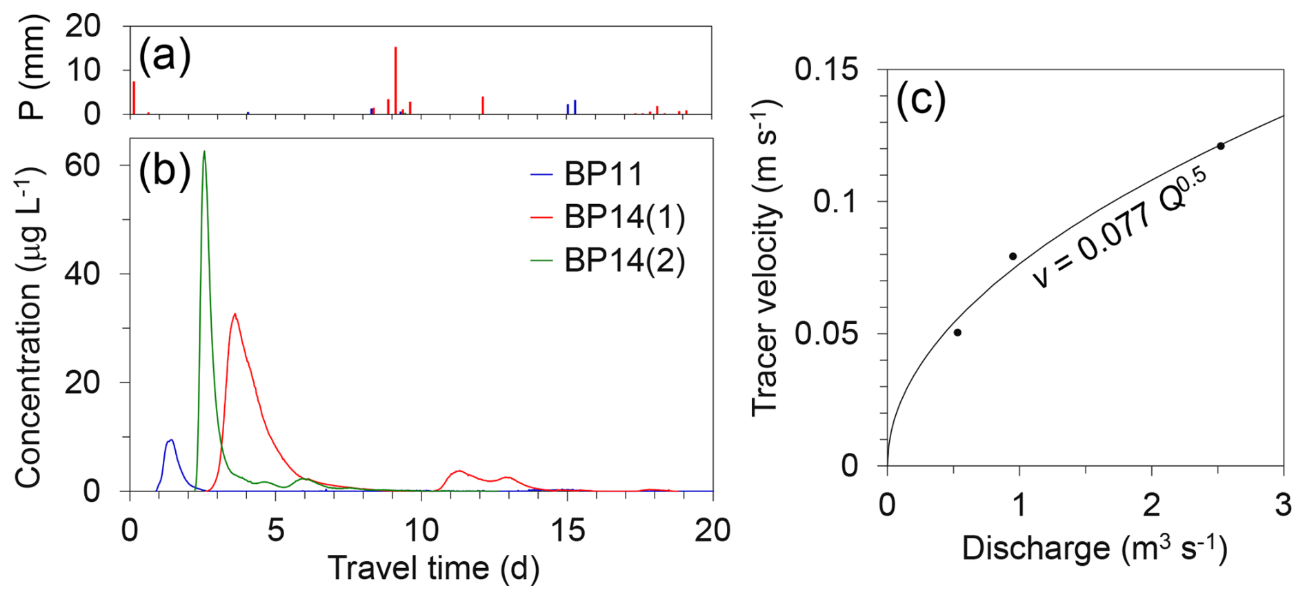
Figure 5 (a) Six-hour precipitation recorded at Burstall Pass AWS during dye tracer tests. (b) Breakthrough curves for the three dye tracer tests. Estimated tracer concentration is plotted against the time since the tracer release to the conduit system. (c) Relation between spring discharge and mean tracer velocity during the three dye tracer experiments, calculated with a sinuosity factor (S_F) of 1.4. The solid line indicates a power function determined by the least-squares regression. The leading coefficient of the function changes to 0.070 and 0.093 when S_F=1.2 and 1.6, respectively, are used.

4 Results

4.1 Dye tracer tests

Each tracer test captured a complete break through curve (Fig. 5b) demonstrating the connection between the tracer release points and the WKS. The tracer release at BP11 took place on 14 July 2022, during active snowmelt. The tracer was dissolved in snowmelt water and poured into the pit, where a visually estimated flow rate of 0.05 L s⁻¹ was entering the shaft. Due to the scarcity of naturally flowing water, some dye losses were anticipated. The BP14(1) tracer test was conducted on 17 September 2021, during a brief period of low air temperature (Fig. 6a) that halted the flow of glacial meltwater into the swallet. Water from nearby puddles was used to dissolve the dye prior to injection and was followed by approximately 760 L of additional water in an attempt to flush the dye to the water table, and the cold period was followed by a warm storm event with 24 mm of rain in 30 h (Fig. 6a). The BP14(2) tracer test was conducted on 30 August 2022, while meltwater was actively draining into the swallet, allowing for immediate flushing of the dye, and potentially reducing dye losses. Water temperature remained stable throughout the monitoring period (Fig. 6b) and turbidity was not noticeable during the tracer tests.

Figure 6 (a) Daily total precipitation and daily mean air temperature measured at the Burstall Pass weather station, 1 April–31 October 2021. (b) Water temperature at the spring outlet. (c) Spring discharge and electrical conductivity (EC). (d) Spring discharge and EC during 8 July–8 August 2021.

A fluorometer calibration was conducted in the field on 22 April 2022 and yielded a calibration coefficient of 0.16 µg L⁻¹ per mV. Laboratory calibrations were also attempted after completing all tracer tests, but gave inconsistent values of calibration coefficients. Due to these discrepancies, there is low confidence in the accuracy of the calibration coefficient, and meaningful analysis of tracer data could only be conducted in a qualitative manner. Nevertheless, the coefficient determined in the field test (see above) was used to convert the sensor mV output to tracer concentration, which were used to calculate tracer travel time and velocities, adjusted for S_F ranging from 1.2 to 1.6 (Eq. 3). The breakthrough curves for BP14 tests had secondary peaks (Fig. 5b) indicating that a small fraction of tracers likely traveled through multiple flow paths having varying transport velocity, possibly reflecting the effects of retardation processes to be discussed later. Due to the uncertainty in the calibration coefficient, it was impossible to determine mass recovery ratios with confidence.

Table 1 Summary of dye tracer tests: BP14(1), BP14(2), and BP11.

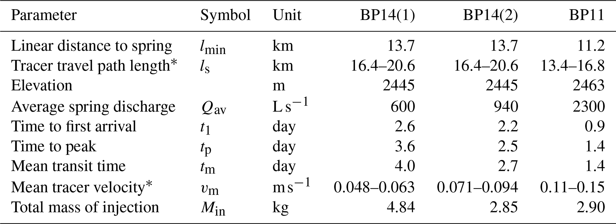
^∗ Upper and lower bounds represent a range of values corresponding to the expected range of sinuosity factor ($\mathrm{1.2}\le S_{\mathrm{F}}\le \mathrm{1.6}$).

Results of the three tracer tests are summarized in Table 1. Given that the tracer was released to actively flowing water at an entrance of the conduit system in both BP14(2) and BP11 tests, the actual time of release was used to indicate the start of these tests. For BP14(1), it was expected that the tracer was retained in the unsaturated part of the conduit system until a heavy storm on the following day flushed it into the actively flowing conduit system (Fig. 5a). Therefore, the end of the storm event was used to indicate the start of the test. This is reflected in the calculation of tracer travel time in Table 1. Tracer velocity increased with average spring discharge during each test as expected (Fig. 5c). The velocity appeared to be linearly related to the square root of discharge, and a power function was used to estimate the transport velocity (v, m s⁻¹) of the system from discharge Q (m³ s⁻¹):

$$\begin{array}{}\text{(5)}& v=a{Q}^{\mathrm{0.5}}\end{array}$$

where a is an empirical coefficient taking a value of 0.077 m${}^{-\mathrm{1}/\mathrm{2}}$ s${}^{-\mathrm{1}/\mathrm{2}}$ for an intermediate value of S_F (=1.4) within the expected range.

4.2 Recharge area delineation

The potential recharge area of the WKS was first delineated from the geological map strata (McMechan, 2012). The area is geologically confined to the Palliser Fm. within a regional syncline, with the underlying Sassenach Fm. acting as an aquitard. The area must extend to Mt. Sir Douglas based on the tracer test, giving a geologically possible extent of catchment (36 km²) indicated in Fig. 1. However, not all the geologically defined area is expected to contribute meaningful amounts of recharge. Snowmelt and rain on steep bedrock cliffs and slopes quickly becomes overland flow, which must be retained in relatively flat areas, where it infiltrates rapidly into the karst system. Forested valley floors with perennial streams are groundwater discharge areas and unlikely to serve as effective recharge area. Using these as a guide, likely recharge area is further constrained to 18 km² as indicated in Fig. 1. This gives a rough estimate of the effective catchment of the WKS.

The feasibility of the catchment estimated above is evaluated using a simplified annual water balance:

$$\begin{array}{}\text{(6)}& A_{\mathrm{C}}=V/[P-(\mathrm{ET}+S)-R]\end{array}$$

where A_C is the catchment area (m²), V is the total volume of discharge at the WKS (m³), Pis precipitation (m), ET is evapotranspiration (m), S is snow sublimation (m), and R is surface runoff (m). The average annual water balance was calculated using the data from hydrological years 2017 to 2023, where a hydrological year is defined as 1 November–31 October because snow accumulation usually starts in late October.

Using the data from Burstall Pass AWS, P was estimated to be 1183 mm though this value has some uncertainty associated with the spatial variability of precipitation within the catchment (see Sect. 3.3). Evapotranspiration and sublimation, while not directly measured in this study, were estimated as follows. Direct measurement of ET and S in alpine catchments are rare in the Canadian Rockies, but Hood and Hayashi (2015) examined the detailed water balance of an alpine catchment at the Lake O'Hara study site located 80 km northwest of the WKS and determined average annual discharge of Opabin Creek in 2007 and 2008 to be 1110 mm, whereas average annual precipitation was 1190 mm (He and Hayashi, 2019). The difference is attributed to ET +S, and most of it is likely S because ET during the snow-free period (∼3 months) from mostly non-vegetated catchment is expected to be minimal. MacDonald et al. (2010) examined sublimation in an alpine sub-catchment of the Marmot Creek basin located 20 km east of the WKS and estimated the mean annual sublimation in 2007 and 2008 to be 80 mm. These studies give a rough estimate of ET+S as 80 mm. It is difficult to estimate R, but Lilley (2023) estimated total annual runoff of ∼20 mm in 2021 in Burstall Creek draining the central part of recharge area (Fig. 1a). Using a rough estimate of 80 mm for ET+S and 20 mm for R, Eq. (6) gives A_C≅17 km², which is similar to the estimate of 18 km² based on geology and topography. While these estimates have a large degree of uncertainty, A_C=18 km² is used in the catchment water balance calculations in Sect. 4.8. The high recharge-to-precipitation ratio (∼0.92) estimated above is consistent with high values (0.8–0.9) reported for the karstic terrain in the Helvetic Alps in Switzerland (Malard et al., 2016).

4.3 Seasonal dynamics of spring discharge, water temperature, and EC

The seasonal dynamics of spring discharge, water temperature, and EC were consistent between 2020 and 2021. Only the 2021 data are described here, while the 2020 data are shown in the Appendix (Fig. A1). As air temperature rose in the Spray Mountains during April and May (Fig. 6a), the rapid transmission of snowmelt from the catchment area was indicated by substantial increases in discharge of up to 1600 L s⁻¹ during 15–18 May (Fig. 6c). Decreases in both water temperature and EC indicated snowmelt dilution (Fig. 6b and c). Diel fluctuations in discharge and EC (Fig. 6d) caused by diurnal snowmelt were observed from the beginning of the snowmelt season until late September.

Noticeable changes in the behaviour of discharge and EC occurred around 18–23 July, when the magnitude of diel fluctuations of discharge decreased and that of EC increased (Fig. 6d). As the discharge receded and dropped below 1000 L s⁻¹, the discharge recession slope flattened, and EC began rising towards stable winter levels. Therefore, this appears to define a transition point in the hydrochemical behaviour of the system, and hereafter is referred to as the “hydrochemical transition point”. A similar hydrochemical transition point was observed around 10–15 August 2020 at a discharge value of 1000 L s⁻¹ (Fig. A1).

4.4 Magnitude and phase of diel fluctuations

The magnitude of diel fluctuations of discharge and EC had distinct seasonal patterns (Fig. 7b). The magnitude for discharge fluctuations was large during the high-flow period, equivalent of 3 %–9 % of the daily mean discharge, and decreased to less than 1 % of the mean discharge around the hydrochemical transition point of 18–23 July. In contrast, the magnitude of EC fluctuations was relatively small, equivalent of 1 %–2 % of the daily mean EC, and increased rapidly after the hydrochemical transition point, reaching a maximum of ∼5 % of the daily mean EC.

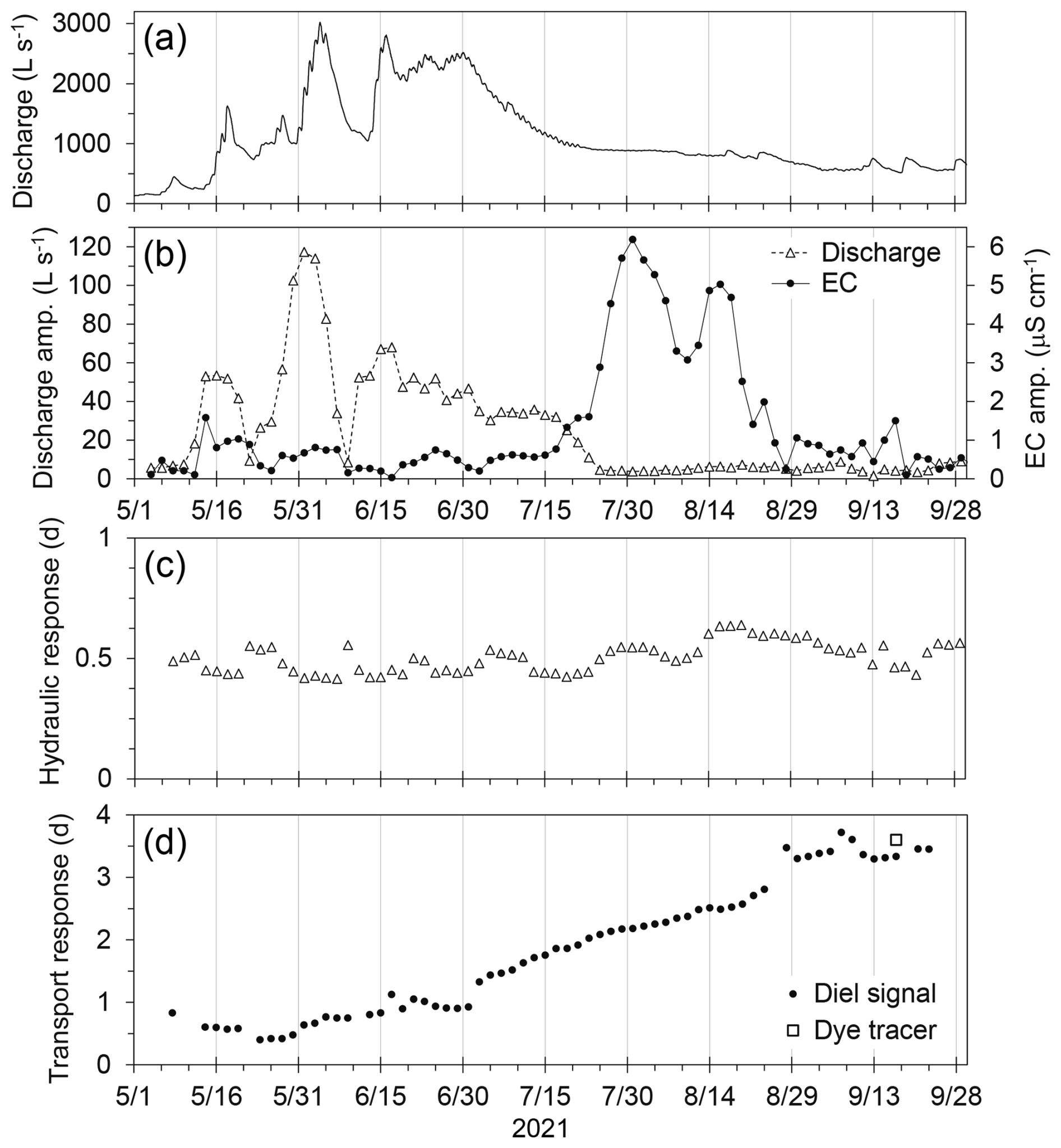
Figure 7 (a) Spring discharge during 1 May–30 September 2021. (b) Amplitude of diel fluctuations of spring discharge and electrical conductivity (EC) during the same period. (c) Hydraulic response time of spring discharge determined by the analysis of diel fluctuations. (d) Transport response time of EC to diurnal snowmelt (i.e. diel signal) and the dye tracer travel time determined using the peak concentration arrival.

Diel fluctuations of discharge had a phase delay of approximately 0.5 d compared to air temperature throughout the entire season (Fig. 7c), meaning that the hydraulic response of the spring to diurnal snowmelt inputs was nearly constant. In contrast, the phase delay of EC gradually increased and reached ∼3.5 d in September (Fig. 7d), meaning that the transport response time of the spring became longer. The transport response time determined by the phase analysis was consistent with the result of the dye tracer test (Fig. 7d). Note that the travel time of peak tracer concentration, not the center of mass, is used in the figure. This is necessary because the phase lag is determined from the analysis of concentration data alone, not the product of concentration and discharge (i.e. mass flux).

4.5 Chemical and isotopic composition

The chemical composition of all spring water samples was dominated by Ca and Mg (>98 % of total cations in meq L⁻¹) and alkalinity and SO₄ (>99 % of total anions). Since the pH of all samples ranged between 7.68 and 7.82, essentially all alkalinity is attributed to HCO${}_{\mathrm{3}}^{-}$ (Domenico and Schwartz, 1998, p. 257). Therefore, concentrations of the four ions (Ca²⁺, Mg²⁺, HCO${}_{\mathrm{3}}^{-}$, and SO${}_{\mathrm{4}}^{\mathrm{2}-}$) represent the hydrochemical dynamics of the spring. In general, concentrations of the four ions decreased during the high-flow period due to dilution of over-winter storage with fresh snowmelt water (Fig. 8a). However, changes in concentration were asynchronous among the ions, resulting in different ratios of cations and anions over the season.

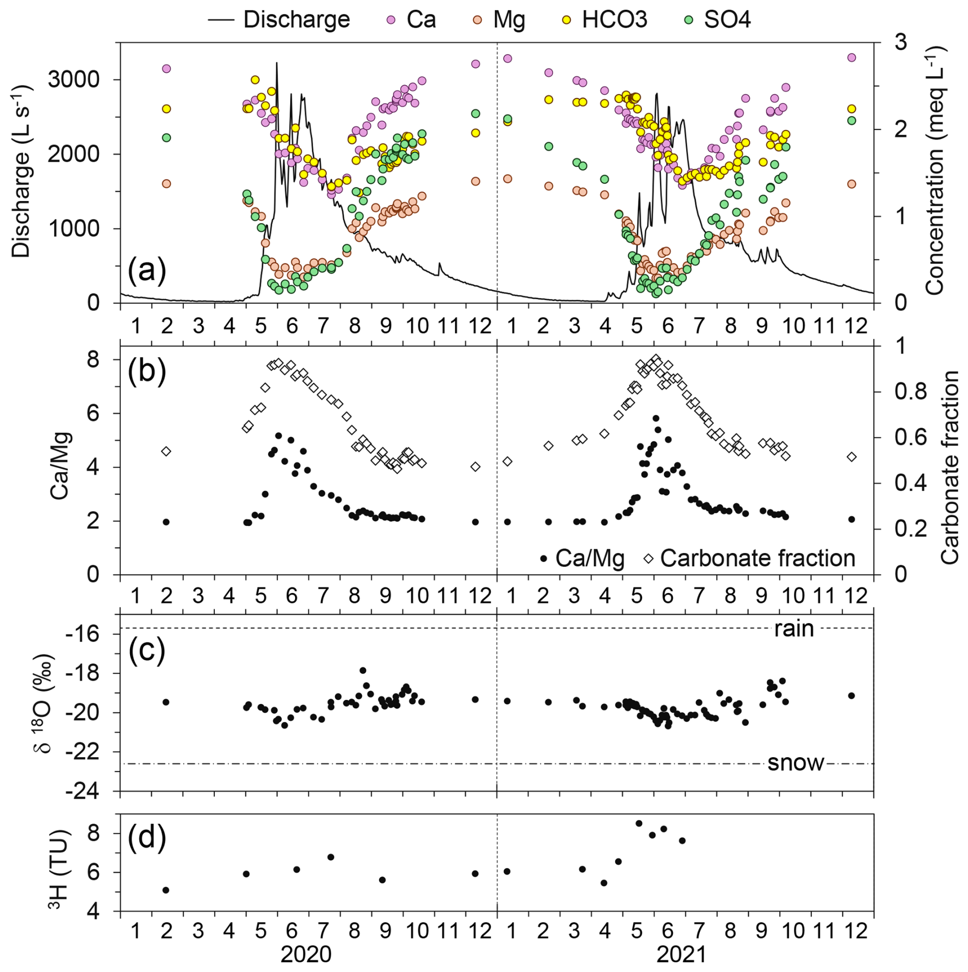
Figure 8 (a) Spring discharge and concentrations of dominant ions during January 2020 to December 2021. (b) The Ca-to-Mg ratio and carbonate fraction of spring water. (c) Oxygen stable isotope ratio of spring water. Horizontal lines indicate the mean isotope compositions of rain and snow samples. (d) Tritium content of spring water.

For example, the $\mathrm{Ca}/\mathrm{Mg}$ concentration (meq L⁻¹) ratio became remarkably constant after the hydrochemical transition point (mid-August in 2020 and mid-July in 2021) and remained constant until snowmelt (Fig. 8b). The carbonate fraction, $\left[{\mathrm{HCO}}_{\mathrm{3}}^{-}\right]/\left(\right[{\mathrm{HCO}}_{\mathrm{3}}^{-}]+\mathrm{2}[{\mathrm{SO}}_{\mathrm{4}}^{\mathrm{2}-}\left]\right)$, also had a distinct seasonal pattern (Fig. 8b), where [ ] indicates molar concentration. These suggest that there are at least two types of groundwater in the system: the over-winter component having a constant $\mathrm{Ca}/\mathrm{Mg}$ ratio (=2) and relatively high ion concentrations, and the component associated with snowmelt recharge having a higher $\mathrm{Ca}/\mathrm{Mg}$ ratio and carbonate fraction but lower ion concentrations. It is impossible to perform quantitative endmember mixing analysis of the two components because all four species are reactive, however, the information is useful for qualitative understanding of the groundwater system.

Based on the geologic setting (Fig. 1a), the spring water likely derives its chemical contents from the minerals in the Palliser, Banff, and Exshaw Fms. through the dissolution of calcite, dolomite, anhydrite, and pyrite. The saturation indices (in logarithmic scale) of spring waters ranged between −0.9 and 0.1 for calcite, −2.6 and −0.4 for dolomite, and −2.9 and −1.9 for anhydrite, where the highest values occurred during December–March and the lowest values occurred during the high-flow period. A preliminary calculation shows that attributing all dissolved SO₄ to anhydrite (CaSO₄) does not leave enough Ca to account for the release of Mg from the dissolution of dolomite or magnesian calcite. Therefore, part of SO₄ must come from the dissolution of magnesium-sulfate minerals or the oxidation of pyrite. This will be examined further in the discussion.

Isotopic compositions of rain and snow samples plotted along a straight line (Fig. A2) defining the local meteoric water line (LMWL) of: δ²H = 7.55 (±0.08) ×δ¹⁸O + 0.03 (±1.54), where bracketed numbers indicate 95% confidence intervals. It was not possible to calculate volume-weighted mean compositions, but arithmetic mean compositions (δ¹⁸O, δ²H) of all samples were ($-\mathrm{15.7}\pm \mathrm{2.7}$, $-\mathrm{119}\pm \mathrm{22}$) for rain and ($-\mathrm{22.6}\pm \mathrm{1.2}$, $-\mathrm{170}\pm \mathrm{9}$) for snow, where the uncertainty indicates one standard deviation. The spring water samples also plotted along the LMWL and had relatively small seasonal variability, as demonstrated by δ¹⁸O values shown in Fig. 8c. They were mostly constrained between −20.5 ‰ and −18.5 ‰, and deviated only slightly from the average value of −19.7 ‰ during the high-flow periods, when the chemical compositions responded strongly to the influx of snowmelt recharge (Fig. 8b). The difference between chemical and isotopic behaviours of spring water will be examined further in the discussion.

The spring water had moderately high tritium content indicating post-1950 recharge (Fig. 8d). The values did not have obvious seasonal pattern in 2020, but the tritium content appeared to increase during the high-flow period in 2021. The nearest available long-term data of tritium in precipitation are from Ottawa, located ∼3000 km east of the WKS (IAEA, 2025). The tritium content in precipitation during 1995–2019, corrected for radioactive decay (half life = 12.3 years) to January 2021, had substantial seasonal and inter-annual variability (Fig. 9), and gradually increased from 3–10 TU in the late 1990s to 8–15 TU in recent years. It is impossible to determine the residence time of water, considering the possible variability of tritium contents between Ottawa and the WKS, but in an approximate sense, it seems likely that most spring water samples had a residence time of five to ten years.

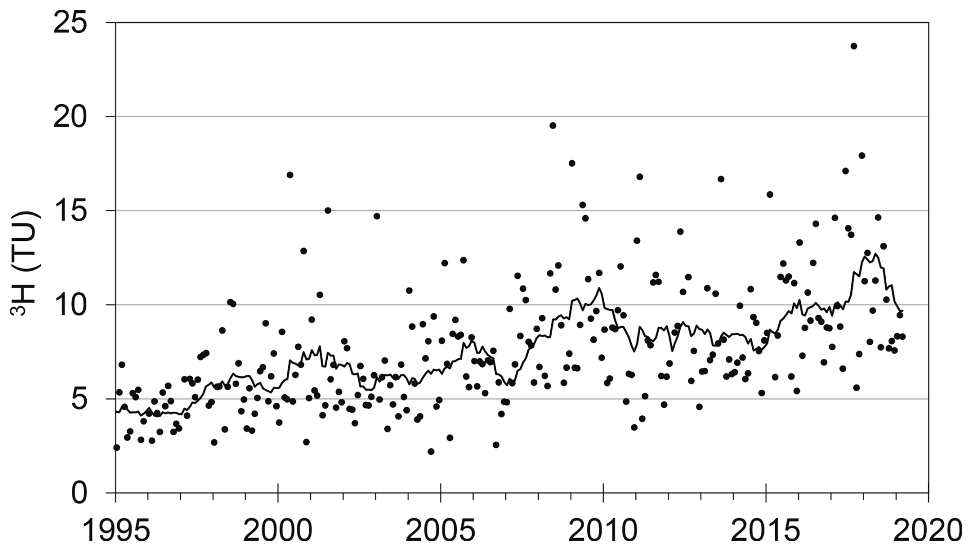
Figure 9 Tritium content in precipitation monitored in Ottawa, Canada (IAEA, 2025). The values are corrected for radioactive decay to January 2021. The line indicates backward 12-month moving average.

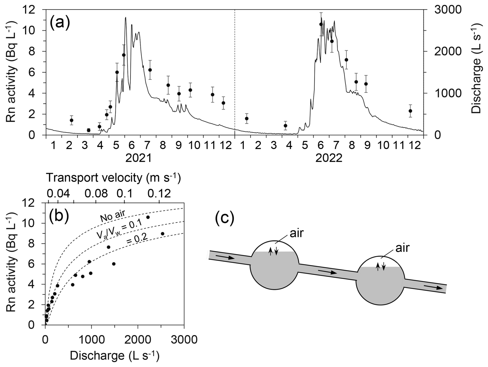
Figure 10 (a) Spring discharge and the activity of dissolved ²²²Rn in spring water. Error bars indicate the analytical uncertainty. (b) Relation between spring discharge and ²²²Rn activity. Dashed line indicates the theoretical decay curve for the initial activity of 15 Bq L⁻¹ for cases with no air in the system, and air-to-water volume ratio ($V_{\mathrm{a}}/V_{\mathrm{w}}$) of 0.1 and 0.2. The top horizontal axis shows transport velocity calculated from discharge using Eq. (5). (c) Conceptual model of ²²²Rn transport in the karst system consisting of water-saturated conduits and partially air-filled chambers, where the air-water exchange of ²²²Rn takes place.

4.6 Dissolved radon activity

The activity of dissolved ²²²Rn had a distinct seasonal pattern similar to discharge (Fig. 10a), however, relatively high ²²²Rn activity (>2 Bq L⁻¹) was sustained into early winter even after discharge decreased to low values (<500 L s⁻¹). This is similar to seasonal patterns observed in cave systems in Switzerland (Eisenlohr and Surbeck, 1995) and Italy (Peano et al., 2011).

Carbonate minerals forming limestone and dolomite generate relatively little ²²²Rn due to a lack of ²²⁶Ra distributed on mineral surfaces (Eisenlohr and Surbeck, 1995). However, weathered fragments of Palliser limestone can generate sizable ²²²Rn inputs as indicated by a laboratory experiment using talus deposits consisting of Palliser limestone in a previous study (Christensen et al., 2020) at the Hathataga Creek catchment located ∼16 km east of the WKS (Fig. A4). The accumulation of ²²²Rn in initially ²²²Rn-free water is described by Hoehn et al. (1992); also Appendix B:

$$\begin{array}{}\text{(7)}& A\left(t\right)=A_{\mathrm{e}}[\mathrm{1}-\exp (-\mathit{\lambda }t\left)\right]\end{array}$$

where A(t) is the ²²²Rn activity (Bq L⁻¹) at time t (d), A_e is the ²²²Rn activity at steady state with ²²⁶Ra, and λ is the radioactive decay constant of ²²²Rn (=0.18 d⁻¹). Equation (7) indicates that the infiltrating water (i.e. recharge flux) needs to reside in ²²⁶Ra-containing soil or weathered rock for 13 d to reach A(t)>0.9A_e if the material is completely saturated, and much longer if the material contains some air. This gives a qualitative constraint on the minimum transit time of snowmelt or rainwater before it enters the karst conduit network.

Once the water is in the conduit network, where little addition of ²²²Rn occurs due to low ratio of rock surface area to water volume (Appendix B), dissolved ²²²Rn undergoes exponential decay with a half life of ∼3.8 d. Therefore, longer transit time in the conduit network will result in lower ²²²Rn activity. Using the discharge-velocity relation estimated from the tracer tests (Eq. 5) and assuming a linear distance of 12 km between the recharge area and the spring and S_F=1.4, theoretical ²²²Rn activities at the spring for different discharge values are shown in Fig. 10b (line labeled “No air”). An initial ²²²Rn activity of 15 Bq L⁻¹ is used in the calculation, based on the values observed at a non-karst spring discharging from a moraine aquifer containing Palliser limestone at Hathataga Creek, where an approximate residence time of groundwater was determined to be 50–100 d using a dye tracer (He and Hayashi, 2023). The observed ²²²Rn activities plot far below the no-air line at low to medium discharge suggesting additional loss of ²²²Rn by degassing.

Radon has a relatively high Henry's law constant of $N_{\mathrm{a}}/N_{\mathrm{w}}\approx \mathrm{4.5}$, where N_a and N_w are molar concentrations in air and water, respectively (SRNL, 2017). To gain qualitative understanding of the effects of degassing, an analysis is performed using a simple transport model in water-air system consisting of water-saturated conduits and partially air-filled chambers (Fig. 10c). Air and water phases are in equilibrium with respect to ²²²Rn activity while dissolved ²²²Rn travels at a constant velocity. The equilibrium assumption is justified considering a rapid air-water exchange rate of dissolved ²²²Rn (Peano et al., 2011). In a field experiment on 29 June 2021, a water sample collected ∼30 m downstream of the outlet spring had only ∼20 % of ²²²Rn activity compared to the samples collected at the spring, indicating substantial degassing over a short distance. The transport and decay of ²²²Rn in a moving packet of water (i.e. Lagrangian transport) is described by:

$$\begin{array}{}\text{(8)}& {\displaystyle \frac{\mathrm{d}A}{\mathrm{d}t}}=-\mathit{\lambda }\left(\mathrm{1}+H_{\mathrm{c}}{\displaystyle \frac{V_{\mathrm{a}}}{V_{\mathrm{w}}}}\right)A\end{array}$$

where A is ²²²Rn activity in water, H_c is the dimensionless Henry's law constant, and $V_{\mathrm{a}}/V_{\mathrm{w}}$ is the average air-to-water volume ratio in the karst system. Integrating Eq. (8) over the transport time between the recharge area and the spring, the final ²²²Rn activities for different discharge values are plotted in Fig. 10b for $V_{\mathrm{a}}/V_{\mathrm{w}}=\mathrm{0.1}$ and 0.2. While this approach is simplistic, it demonstrates that the observed ²²²Rn activity is influenced by degassing and that a relatively small volume of air in the system is sufficient to make a noticeable difference in ²²²Rn activity.

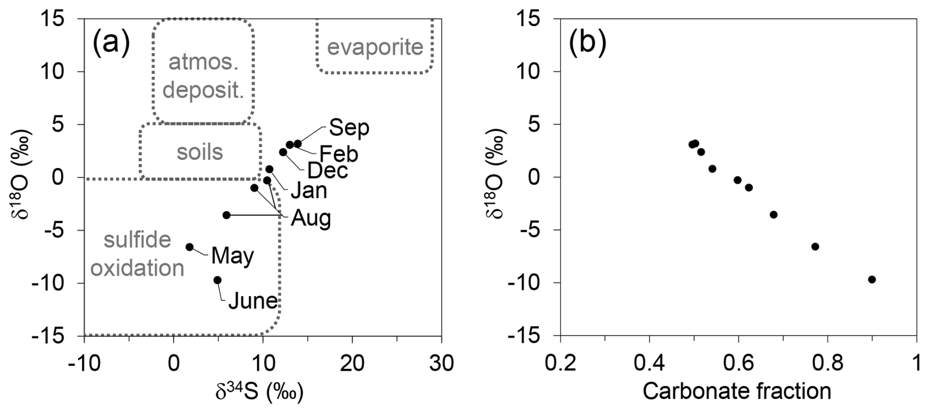
Figure 11 (a) Relation between stable isotope ratios of sulfur (δ³⁴S) and oxygen (δ¹⁸O) in dissolved sulfate in spring samples during August 2021 and September 2022, with dashed lines indicating the composition fields of potential sulfate sources (Nightingale and Mayer, 2012). (b) Relation between carbonate fraction in water and δ¹⁸O in sulfate.

4.7 Isotopic composition of sulfate

The stable isotopic signatures of dissolved SO₄ in spring water showed a seasonal trend, whereby the samples collected during spring freshet had lower values of δ³⁴S and δ¹⁸O compared to the samples from late summer and winter (Fig. 11a). These values are compared to the signatures of different sulphate sources delineated by Nightingale and Mayer (2012) based on a comprehensive literature review of studies investigating the isotopic composition of sulphate in precipitation, river and lake water, groundwater, soils, and rocks. The evaporite field was further constrained to the typical isotopic signatures of Devonian carbonates (δ³⁴S ranging 17 ‰–28 ‰; δ¹⁸O ranging 10 ‰–17 ‰) (Claypool et al., 1980; Grasby, 1997). The seasonal pattern of isotope signature suggests a strong influence of SO₄ derived from the oxidation of sulfide minerals during the snowmelt period and a substantial contribution of evaporite during fall and winter (Fig. 11a).

The δ¹⁸O values of dissolved SO₄ had a linear relation with the carbonate fraction of water (Fig. 11b), suggesting the mixing of two components of water. Since high carbonate fraction was observed during the high-flow period (Fig. 8b), this component represents snowmelt recharge. The component with low carbonate fraction represents groundwater released from over-winter storage, which is presumably in contact with evaporite deposits within the Palliser Fm., similar to observations made by Barna et al. (2020) for a karst system in China.

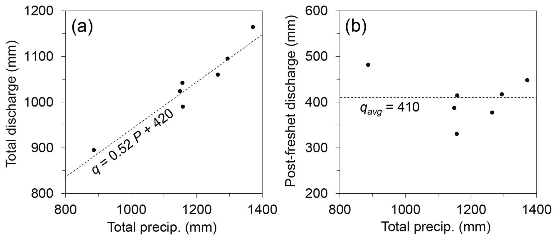
Figure 12 (a) Relation between total precipitation and discharge of hydrological years (1 November–31 October) of 2017–2023, with the dashed line indicating a linear relation determined by the least-squares regression. (b) Relation between total precipitation and the post-freshet discharge after the hydrochemical transition point. The dashed line indicates the average of seven years.

4.8 Annual water balance

To examine the water balance of the karst system, annual precipitation recorded at Burstall Pass AWS was compared against total annual discharge of the WKS for hydrological years 2017–2023. The discharge was expressed in mm by dividing it by the effective catchment area of 18 km² (see Sect. 4.2). Total annual discharge was strongly correlated with annual precipitation (Fig. 12a). This is expected as the majority of discharge occurred during May–August, when the flow was driven by snowmelt and summer rain (Fig. 8a). After this high-flow period, the spring discharge was mostly sustained by the release of groundwater stored within the system.

The amount of storage release can be assessed by examining the amount of post-freshet flow, defined as the total flow between the hydrochemical transition point (see Sect. 4.3) and the beginning of freshet in the following year. There was no obvious correlation between total precipitation and post-freshet discharge (Fig. 12b), suggesting that the total amount of precipitation has relatively little influence on the amount of groundwater stored in the system after the hydrochemical transition point. This can be explained if it is assumed that the hydrological input to the karst system is far greater than the storage capacity, resulting in the full capacity of groundwater at the hydrochemical transition point regardless of the input amount. Similar observations are made in alpine aquifers consisting of Quaternary sediments (Hayashi, 2020). The average of post-freshet flow over seven years was 410 mm (Fig. 12b), which is similar to the intercept (=420 mm) of the linear relation between total precipitation and total discharge (Fig. 12a). It is not clear if this is merely a coincidence, or if it indicates the influence of storage capacity on the annual water balance.

5 Discussions

5.1 Residence time of groundwater

Groundwater flow in karst systems generally consists of a relatively slow component through fractured rock and a fast component through the conduit network (Jourde and Wang, 2023). The residence time of water reflects the combined effects of slow and fast components. The transport response time determined by dye tracer tests and the analysis of diurnal EC fluctuations (Fig. 7d) is controlled by the fast flow through the conduit network, on the order of several days. In contrast, chemical and isotopic compositions of spring outflow (Fig. 8) reflect much slower processes associated with the interaction of rain and snowmelt water with surface sediments and fractured rock before the water enters the conduit system.

Two distinct phases were observed in the system, defined by changes in the flow regime and the chemical composition of water. The first phase occurred during the high-flow period in May–August, when discharge was sustained above ∼1000 L s⁻¹ by snowmelt recharge, and was characterized by high $\mathrm{Ca}/\mathrm{Mg}$ and carbonate fraction (Fig. 8b) and the sulfate isotopic composition influenced by sulfide oxidation (Fig. 11). This likely represents the interaction of snowmelt with calcite-saturated water in sulfide-bearing fractured rocks of Exshaw and Palliser Fms. (Fig. 1) and surface sediments derived from them. The isotopic composition shifted only slightly towards the signature of snowmelt (Fig. 8c) from the over-winter composition, indicating the dominance of water stored in surface sediments and fractured rock for at least a year, most likely longer. This is consistent with the tritium content suggesting a residence time of multiple years (Figs. 8d and 9).

The second phase starts after the hydrochemical transition point when the flow regime shifts from high flow with strong diel fluctuations to low flow with weak diel fluctuations (∼20 July in Fig. 7a and b). The $\mathrm{Ca}/\mathrm{Mg}$ is constant (=2) during the second phase, and carbonate fraction is stable (Fig. 8b). The sulfate isotopic composition of this water is more strongly influenced by anhydrite dissolution compared to the first phase (Fig. 11). It represents the over-winter drainage of water stored in the deeper part of Palliser Fm. The lower $\mathrm{Ca}/\mathrm{Mg}$ ratio during this phase, compared to the first phase, may be indicative of a slower dissolution rate of dolomite than calcite (Barna et al., 2020; Plummer, 1977). The amount of over-winter drainage is consistent from year to year at ∼410 mm (Fig. 12b). Based on the relatively small shift of stable isotopic composition in the first phase, the total over-winter storage is expected to be much greater than 410 mm.

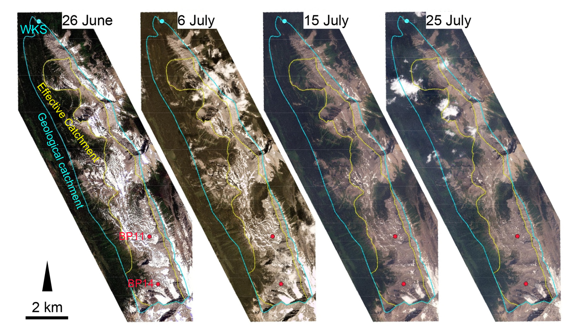
Figure 13 Satellite images of the potential recharge areas of the Watridge Karst Spring (WKS) on 26 June, 6 July, 15 July, and 25 July of 2021. The images show the tracer release locations (BP11 and BP14), the geological catchment, and the effective catchment (Fig. 1a). Image source: Planet Team (2025).

The transition of chemical composition is concurrent with a distinct change in the diel fluctuations of discharge and EC as demonstrated in Fig. 6d, whereby the fluctuation magnitude of discharge decreases and that of EC increases. The timing of transition coincided with the complete disappearance of snow cover from the Burstall Pass plateau near BP11, where a series of satellite images (Planet Team, 2025) indicated that snow cover disappeared between 15 and 25 July (Fig. 13). Similarly, the snow cover disappeared from the plateau between 5 and 12 August in 2020 (Fig. A3), coinciding with the hydrochemical transition (Fig. A1). Therefore, the hydrochemical transition represents the shift of the dominant source of diel signals from widespread snowmelt recharge in the plateau area to point recharge of glacier melt water. The former has a strong influence on discharge fluctuations because the amount is much greater than glacier input, but a weak influence on EC because new snowmelt water is mixed with the old (i.e. over-winter) water before it enters the conduit system. In contrast, the latter sends glacier melt water directly to the conduit and has a stronger influence on EC fluctuations.

5.2 Flow velocity in conduit network

The transport velocity determined by dye tracer tests does not generally represent the actual flow velocity through karst conduits because there are physical processes that can delay the transport of conservative tracers, for example, partial mixing with stagnant pools of water (Zuber et al., 2011). This is commonly referred to as retardation (e.g., Hauns et al., 2001). On the other hand, the hydraulic response time reflects the rate of energy propagation, rather than water itself, and is not directly related to flow velocity. In some literature, the energy propagation rate is referred to as celerity (Worthington and Foley, 2021).

To infer the nature of flow and transport processes from available information, an order-of-magnitude calculation of flow velocity is useful. Groundwater flow in karst conduits generally has a high Reynolds number (>10²–10³) and hence, does not obey Darcy's law (Worthington and Soley, 2017). The flow through conduits is commonly conceptualized as turbulent flow in a pressurized (i.e. confined) conduit using the Darcy-Weisbach equation or open conduit flow using Manning's equation. Inferring from a relatively low air-to-water volume ratio suggested by ²²²Rn data (Fig. 10b), it is assumed that most of the conduit flow occurs under pressurized conditions.

Following the approach of Jeannin (2001), discharge Q_p (m³ s⁻¹) and velocity v_p (m s⁻¹) of turbulent flow through a pressurized conduit are estimated by the Darcy-Weisbach equation:

$$\begin{array}{}\text{(9)}& Q_{\mathrm{p}}=-k^{\prime }{A}_{\mathrm{p}}\sqrt{{\displaystyle \frac{\mathrm{d}h}{\mathrm{d}l}}}\text{ and }{v}_{\mathrm{p}}=Q_{\mathrm{p}}/A_{\mathrm{p}}\end{array}$$

where A_p (m²) is the cross-sectional area, $\mathrm{d}h/\mathrm{d}l$ is the hydraulic gradient, and k^′ (m s⁻¹) is the effective hydraulic conductivity for turbulent flow estimated by:

$$\begin{array}{}\text{(10)}& k^{\prime }=K_{\mathrm{s}}{R}_{\mathrm{h}}^{\mathrm{2}/\mathrm{3}}\end{array}$$

where K_s (m${}^{\mathrm{1}/\mathrm{3}}$ s⁻¹) is a roughness coefficient and R_h (m) is the hydraulic radius equal to A_p divided by wetted perimeter of the conduit. For a circular conduit, R_h is equal to $\mathrm{1}/\mathrm{4}$ of the diameter. It is difficult to estimate the representative hydraulic gradient of the conduit network, however, it can be inferred from previous studies of karst systems in rugged, mountainous terrains similar to the current study. For example, in the Canadian Rockies, a map of the Castleguard Cave (Ford et al., 1983, Fig. 3) suggests a gradient of ∼0.03, and Smart (1988) indicated a gradient ∼0.025 in the Maligne Karst system. Jeannin (2001) indicated gradients ranging 0.0004–0.006 in the flat part of the conduit near the spring outlet in Hölloch cave in Switzerland. Based on these studies, an expected order of the gradient in the WKS system is 0.001–0.01. To obtain a conservative estimate of velocity, $\mathrm{d}h/\mathrm{d}l=\mathrm{0.001}$ is used in the following calculation.

Assuming a K_s of 20 m${}^{\mathrm{1}/\mathrm{3}}$ s⁻¹ (Jeannin, 2001), Eqs. (9) and (10) give Q_p=0.32 m³ s⁻¹ and v_p=0.28 m s⁻¹ for conduit diameter of 1.2 m, and Q_p=2.8 m³ s⁻¹ and v_p=0.5 m s⁻¹ for diameter of 2.7 m. These diameters are smaller than the value of ∼3.7 m measured by a cave diver at the spring outlet (Tom Crisp, unpublished data) but are reasonable, considering the enlargement of conduits connected to the outlet (Maqueda et al., 2023). While this calculation has a large degree of uncertainty, the flow velocity through the pressurized conduit network is expected to be on the order of 0.3–0.5 m s⁻¹ during May–December when Q varies between 0.3 and 3 m³ s⁻¹. A similar calculation for open-conduit flow using Manning's equation gives the same order of velocity for water depths ranging 0.2–1 m. At this magnitude of velocity, water would travel from BP14 to WKS in 10 h during the high-flow period and 20 h during the low-flow period. This is shorter than observed transport response time (Fig. 7d), suggesting the presence of retardation mechanisms. This may include pools within the conduit network that stagnate the flow and cause mixing of water (Hauns et al., 2001), or the time required for infiltrating water to travel through the vadose zone before reaching the main conduit network (see Sect. 5.3). This is consistent with the presence of multiple peaks in tracer breakthrough curves (Fig. 5b). Compared to numerous estimates of transport velocity based on tracer tests (e.g., Ford and Williams, 2007, p. 125), measurements of actual flow velocity are rare. Jeannin (2001) reported velocity measurements of 0.1–1.2 m s⁻¹ for Q ranging 4–8 m³ s⁻¹ at Hölloch cave, which is similar to the order of magnitude calculated above.

5.3 Hydraulic response time

The propagation of hydraulic response in a confined pipe is faster than flow velocity by orders of magnitude (Worthington, 2019), meaning that the diel fluctuations of discharge would have a delay of less than an hour between BP14 and WKS. This is contrary to the observed response time of 12–15 h (Fig. 7c), suggesting that much of the hydraulic response is controlled by processes other than pressure propagation through the conduits. The response time remained nearly constant during May–August, while the infiltration source shifted from snowmelt distributed over a large area to glacier melt further away from the spring. This suggests that the primary control of hydraulic response time may be vertical infiltration of meltwater.

Chemical and isotopic data indicate that the new meltwater is mixed with the old water stored in sediments and fractured rocks before the mixture enters the conduit system (see Sect. 5.1). The rapid response of discharge to meltwater input at a time scale of ∼0.5 d (Fig. 7c) suggests that the mixing of new and old waters occurs in saturated sediments and fractured rocks, and that the increased pressure in the saturated zone drives the mixture into larger openings. Once the water enters the vertical openings within the epikarst zone, it can be transferred rapidly to the lateral conduit network by gravity-driven, cascading flow through the vadose zone. Therefore, it is possible to explain the delayed hydraulic transmission of snowmelt signal on the order of ∼0.5 d by the vertical flow. Similar magnitude of delay of diel discharge fluctuations was reported by Smart and Ford (1986) at a glacier-fed karst spring of Castleguard Cave, located ∼190 km northwest of the WKS.

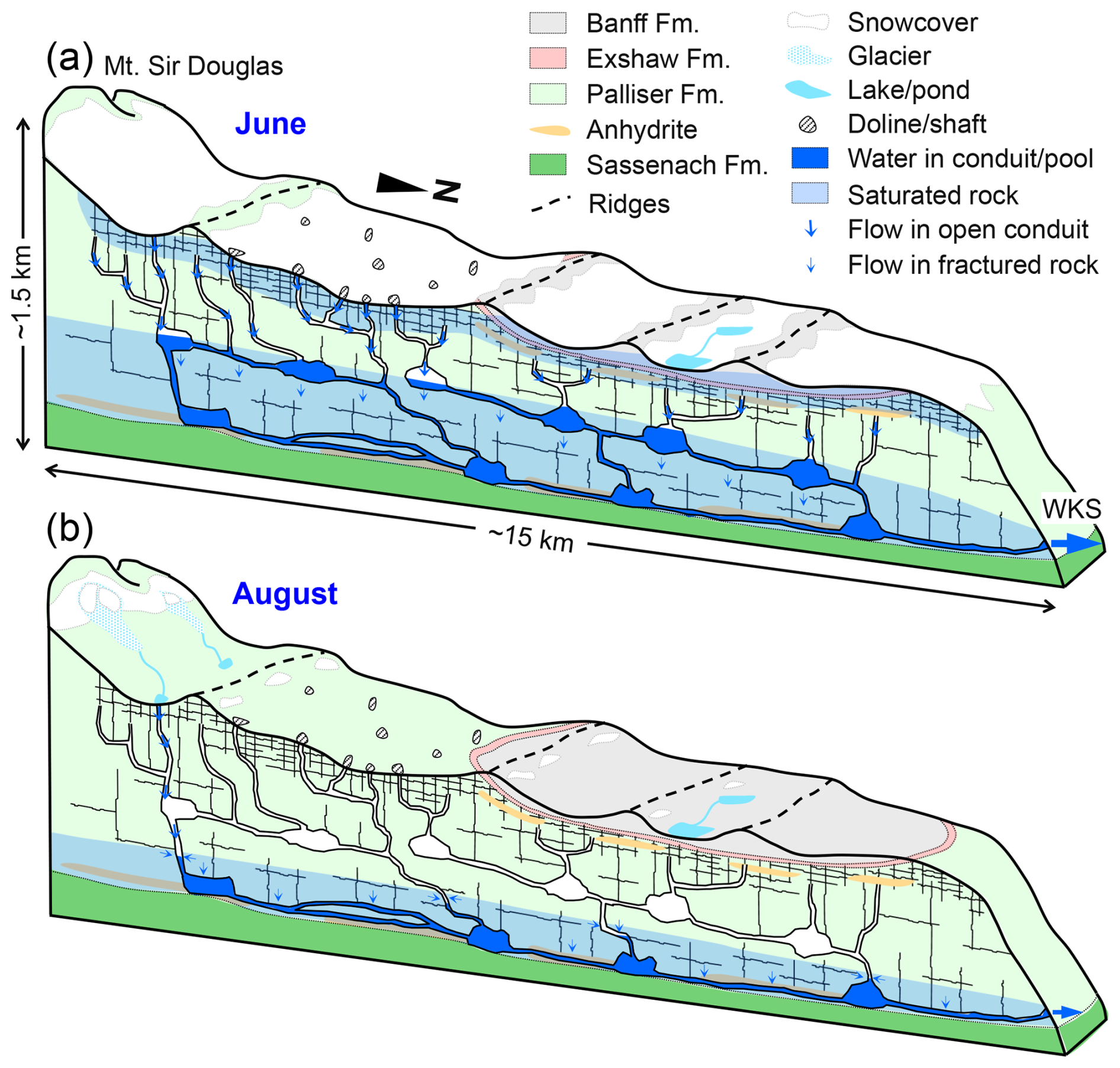
Figure 14 The conceptual cross section of the karst system feeding the Watridge Karst Spring (WKS), showing geological units and possible configuration of conduit network consisting of saturated pipes, open channels, and pools retarding solute transport. (a) Inferred condition during the spring freshet depicting the snowmelt infiltration saturating the epikarst zone. Upper part of conduit system is transmitting snowmelt water rapidly to the saturated conduits. (b) Inferred condition after the hydrochemical transition point depicting the absence of distributed snowmelt infiltration. The remaining groundwater in the deeper zone is gradually drained until the next freshet.

5.4 Conceptual hydrogeological model

The study started with no information on the karst system aside from the location of the WKS. A broad range of data collected over seven hydrological years can now be used to develop a conceptual hydrogeological model (Fig. 14). A reasonably fast arrival of dye tracer plumes clearly shows that the WKS is connected to a network of conduits, yet the transport velocity (0.05–0.15 m s⁻¹) is slower than the order of velocity (0.3–0.5 m s⁻¹) expected for pressurized conduit flow. Therefore, there are likely stagnant pools within the conduit network, causing the physical retardation of solute transport. Two distinct phases of water chemistry indicate mixing of the over-winter component stored in the deeper part of the system (Fig. 14b) with new snowmelt water. Snowmelt is mixed with carbonate-rich water in the epikarst zone (Fig. 14a), resulting in muted diel EC fluctuations. In contrast, the hydraulic signals are conveyed vertically down in the saturated rock and conduits, resulting in pronounced diel discharge signals similar to those observed in non-karst alpine aquifers (e.g., Muir et al., 2011). The transport response time increases over the season as the spring discharge decreases, reflecting the reduction of the overall hydraulic gradient from the high-flow period (Fig. 14a) to the low-flow period (Fig. 14b).

The flow in the conduit network increases downstream from the uppermost part of the catchment (near BP14) to the spring outlet as more water is added through combination of diffuse and point recharge. The conduit network likely includes narrow pressurized parts and open pools retarding solute transport. The karst system likely has multiple levels of conduits (Fig. 14) with bifurcation points as indicated by multiple arrivals of tracer plume (Fig. 5b). The multi-level karst system inferred in this study is consistent with previous alpine karst studies including the karst networks of Crowsnest Pass (Worthington, 1991) and Maligne Canyon (Smart, 1988) in the Canadian Rockies, the Lurbach-Tanneben karst aquifer in Austria (Birk et al., 2014; Kübeck et al., 2013), the Hölloch Cave in Switzerland (Jeannin, 2001), and the Bullock Creek karst aquifer in New Zealand (Crawford, 1989).

6 Conclusions

Rugged and remote terrains are major challenges in alpine karst hydrogeology. This study is an attempt to characterize the hydrogeological behaviour of an alpine karst system, starting from no local information other than the location of the spring outlet. Using geological maps and simple water balance, aided by dye tracer tests at two locations, it was possible to estimate the extent of the catchment of the spring. The dominance of snowmelt in water input provided a unique opportunity to use the diel signal of discharge and electrical conductivity (EC) resulting from distinct diel cycles of snowmelt. The diel signal analysis showed that the solute transport time from recharge areas to the spring (i.e. transport response time) gradually increased over the summer and fall, while the hydraulic response time of discharge remained relatively constant. This implies that the transport response time is controlled by the hydraulic gradient and the magnitude of discharge, while the hydraulic response time is likely controlled by the transmission of snowmelt water through the saturated epikarst zone and vertical openings in the vadose zone to the lateral conduit networks. High-frequency sampling and analysis of chemical and isotopic composition of spring water demonstrated that the karst system is characterized by mixing of over-winter water and seasonal snowmelt water. The isotopic composition of spring water is relatively insensitive to snowmelt input having lighter isotopic composition, indicating that a large volume of water is stored in the fractured rock matrix between the ground surface and the karst conduits. Total discharge volume during the low-flow period after freshet was uncorrelated with annual precipitation, suggesting that the storage volume in rock matrix is large enough to buffer the effects of interannual precipitation variability, and potentially the effects of climate warming affecting the seasonal pattern of precipitation.

The methods developed in this study are expected to be applicable to alpine karst systems in other parts of the world having a distinct snowmelt season generating the diel signals. Combined with geological information, satellite images, and a limited number of tracer tests, the suite of tools presented here can provide an effective approach for characterizing karst hydrogeology in remote terrains. The quantitative analysis in this study was limited to simple differential equations. In the future, more advanced numerical flow and transport models may be used to develop further insights into the possible configuration of the karst system and its response to snowmelt inputs.

Appendix A: Supplementary figures

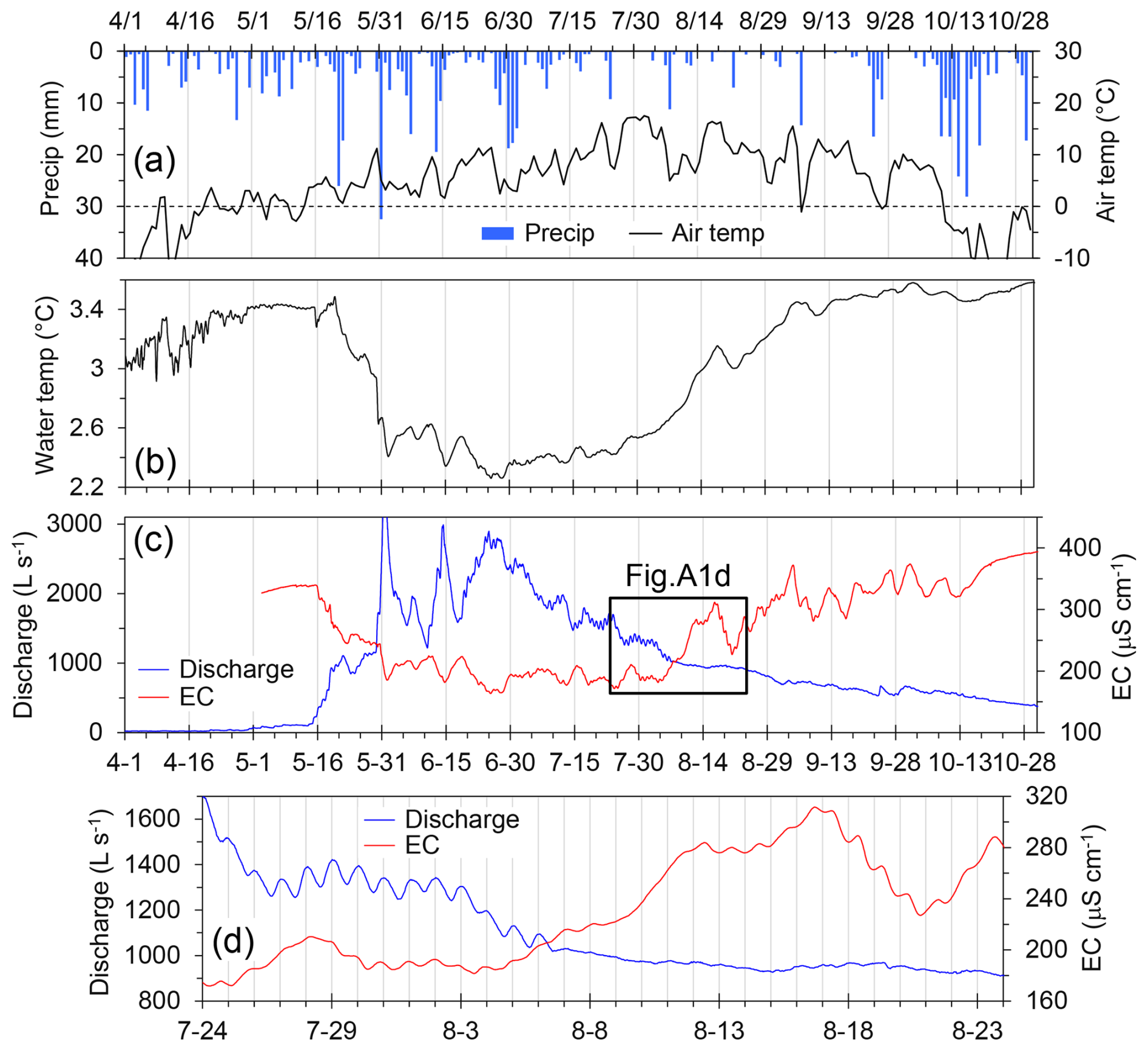
Figure A1 (a) Daily total precipitation and daily mean air temperature measured at the Burstall Pass weather station, 1 April–31 October 2020. (b) Water temperature at the spring outlet. (c) Spring discharge and electrical conductivity (EC). (d) Spring discharge and EC during 24 July–24 August 2020.

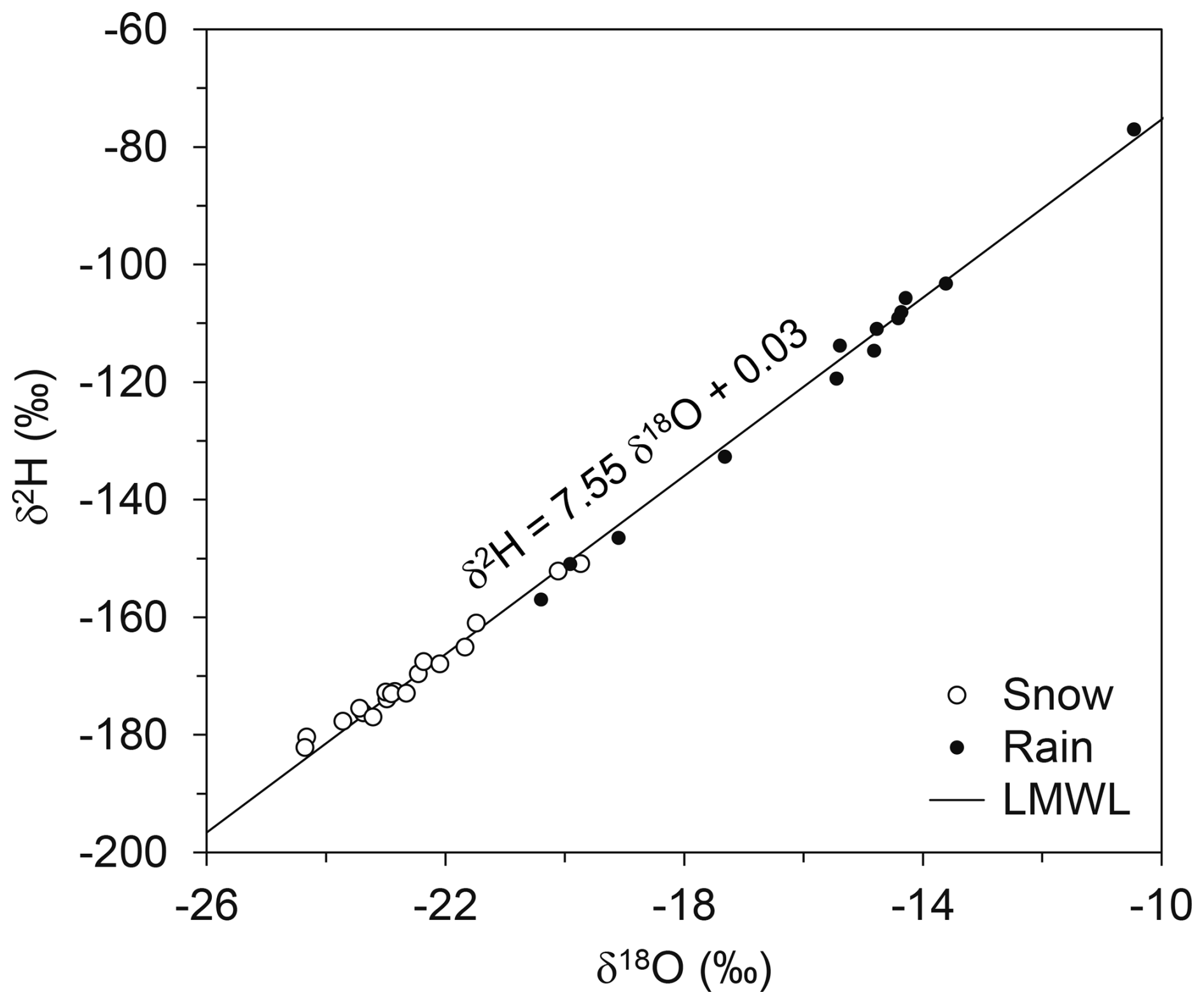
Figure A2 Isotopic composition of rain samples collected at the spring and snow samples collected at the spring or its vicinity (<4 km). The local meteoric water line (LMWL) was derived from all precipitation samples that were collected during this study.

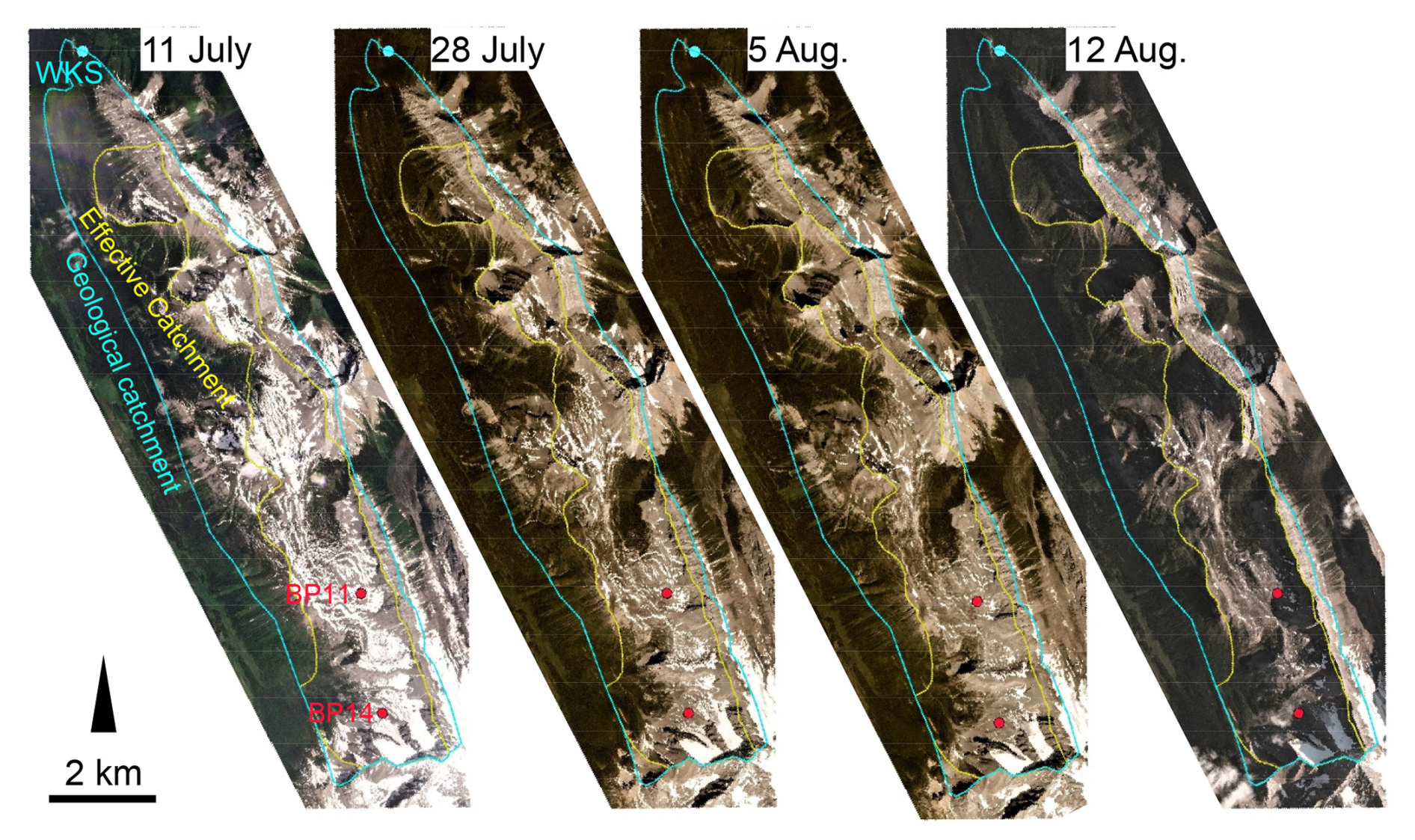
Figure A3 Satellite images of the potential recharge areas of the Watridge Karst Spring (WKS) on 11 July, 28 July, 5 August, and 12 August of 2020. The images show the tracer release locations (BP11 and BP14 the geological catchment, and the effective catchment (Fig. 1a). Image source: Planet Team (2025).

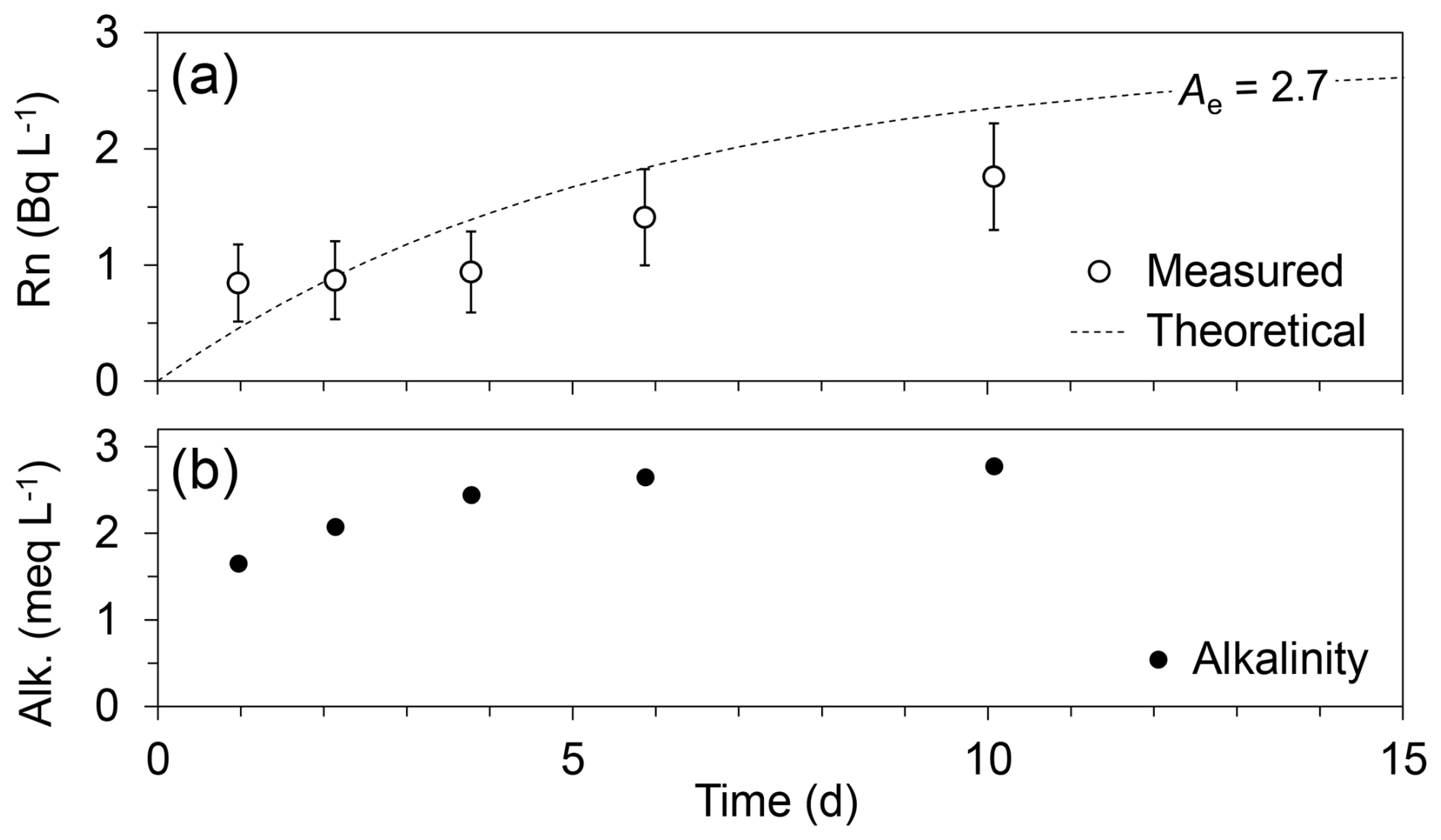
Figure A4 (a) Previously unpublished data of ²²²Rn activity during a laboratory experiment conducted in 2016 using Palliser limestone fragments collected from a talus slope in the Hathataga Creek watershed (Christensen et al., 2020). Error bars indicate the analytical uncertainty. Pebble-sized (diameter 5–30 mm), angular rock fragments were mixed with deionized water in a sealed 2.5 L glass jar and kept in a laboratory at a temperature of ∼22 °C. The porosity of water-rock mixture was 0.45. For each measurement, a 320 mL water sample was collected from the jar and poured back in the jar after the measurement. Prior to the measurements shown in the graph, the same water-rock mixture was left in the laboratory for 147 d to determine the steady-state activity (A_e) of the system. This value is used in Eq. (7) to calculate the theoretical values shown in the graph. Except for the first sample, measured values were lower than theoretical values, most likely due to the loss of dissolved ²²²Rn during measurements. (b) Alkalinity of water samples during the same experiment demonstrating the gradual dissolution of calcite in the initially ion-free water. The equilibrium alkalinity was 6.8 meq L⁻¹.

Appendix B: Equation representing ²²²Rn decay in a closed water-rock system

When a closed system consisting of the rocks containing a source of ²²²Rn is saturated with ²²²Rn-free water, the evolution of ²²²Rn activity (A, Be L⁻¹) can be described by a simple mass balance equation:

$$\begin{array}{}\text{(B1)}& nV{\displaystyle \frac{\mathrm{d}A}{\mathrm{d}t}}=Sf-nV\mathit{\lambda }A\end{array}$$

where n is porosity, V (m³) is the total volume of the system, S (m²) is the total area of rock surfaces emitting ²²²Rn, f (Bq s⁻¹ m⁻²) is the flux density of freshly produced ²²²Rn expressed as the equivalent activity, and λ (s⁻¹) is the decay coefficient. Equation (B1) can be rearranged to:

$$\begin{array}{}\text{(B2)}& {\displaystyle \frac{\mathrm{d}A}{\mathrm{d}t}}={\displaystyle \frac{S_{\mathrm{V}}f}{n}}-\mathit{\lambda }A\end{array}$$

where S_V (m⁻¹) is the volume-specific surface area ($=S/V$). The solution to Eq. (B2) with the initial condition, A=0 at t=0, is:

$$\begin{array}{}\text{(B3)}& A\left(t\right)=(S_{\mathrm{V}}f/n)[\mathrm{1}-\exp (-\mathit{\lambda }t\left)\right]\end{array}$$

which reduces to

$$\begin{array}{}\text{(7)}& A\left(t\right)=A_{\mathrm{e}}[\mathrm{1}-\exp (-\mathit{\lambda }t\left)\right]\end{array}$$

by equating the leading term with A_e (Bq L₋₁), which is the ²²²Rn activity at steady state (Hoehn et al., 1992, Eq. 1). Therefore, for water-rock systems consisting of a particular type of rock (e.g., Palliser limestone) having a similar ²²²Rn flux density, A_e generally increases as specific area increases and porosity decreases.