The potential of green infrastructure in urban pluvial flood mitigation – a scenario-based modelling study in Berlin

Urban surface sealing limits infiltration and thus increases the formation of runoff during heavy rain events. Green infrastructure (GI) measures can be used to reduce urban flood risk by promoting decentralized infiltration and water storage. With a scenario-based modelling study, we investigate the impact of GI on urban runoff formation, flood water depths and the resulting damage to buildings; comparing it with the impact of the conventional drainage system. The study area is located in the city of Berlin, in a heavily sealed 3.3 km² urban catchment. Design rain storms with a duration of one hour and totals between 15 and 100 mm are considered. The GI scenarios include different spatial extents and combinations of bioretention systems, green roofs and pervious pavement. The Storm Water Management Model is used for the urban runoff generation and the 2D-hydrodynamic module of TELEMAC for surface runoff concentration. Building damage is modelled with the Flood Damage Estimation Tool, a recursive partitioning tool developed with survey data representative of building damage caused by pluvial floods. Flood mitigation is investigated regarding absolute and relative reduction and also space efficiency of the GI types. Relative flood mitigation reduces at all modelling steps with increasing rain totals. In contrast, absolute runoff reduction increases with increasing rain totals while the area with maximum water level > 10 cm decreases the most at the 49 mm event and building damage reduces most at 25–30 mm. Bioretention systems achieve the highest spatial efficiency, however, green roofs and pervious pavements do not impede the former land use.

1 Introduction

Pluvial flooding is a ubiquitous risk in urban areas, as heavy surface sealing of urban environments inhibits infiltration and leads to increased and accelerated runoff concentration (Fletcher et al., 2013). Different from fluvial (riverine) flooding, urban pluvial flooding in this study refers to flood events in urban environments, mostly triggered by high-intensity convective rain events of small spatial extent and short duration, which surpass the capacity of the urban drainage system (Paprotny et al., 2021).

Negative pluvial flood impacts include damage to buildings, household goods and infrastructure, causing economic losses, temporally affected mobility and threats to human safety, including physical and psychological health (Berghäuser et al., 2021). Overloaded and damaged sewer systems are further consequences of pluvial flooding from which problems for the environment and human health arise (Owolabi et al., 2022).

In many regions worldwide, an increase in frequency and intensity of heavy rain events has been observed and is expected to continue as a consequence of climate change (Caretta et al., 2022). As pluvial floods are triggered by heavy rain events, this also increases the hazard of pluvial floods.

The increase of heavy rain events can also be observed in Germany (Bürger et al., 2019, 2021). According to the heavy rainfall portal of the German Working Group on Water Issues of the Federal States and the Federal Government (LAWA Starkregenportal; LAWA, 2025), there were 13 events with return periods of 50 to over 100 years with the event maximum in Berlin in the period from 2002–2021. The longest of these events was the event of 28 June 2017 with a duration of 48 h. With an area of 43 058 km² it had also clearly the largest spatial extent and with a rain total of 187.1 mm the highest event total. The remaining events had durations of 1–6 h, with rain totals ranging from 44–109 mm and spatial extents of 15–514 km². The longest return period was attributed to the event of 25 August 2006 with a duration of 2 h, rain total of 109 mm and a spatial extent of 44 km². Pluvial flood damages of residential buildings in Berlin during the same period (2002–2021) summed up to EUR 174  million, with 148 per 1000 residential buildings being affected (GDV, 2023).

Regarding water quality, also smaller rain events matter. The city centre of Berlin has a combined sewer system that conveys wastewater and stormwater together, which is very common in old European cities (Owolabi et al., 2022). When the capacity of the combined sewer system is overloaded due to heavy rainfall, combined sewer overflow (CSO) occurs. This means the release of untreated wastewater to the surface water bodies, deteriorating water quality (Owolabi et al., 2022; Weyrauch et al., 2010). Riechel et al. (2016) found that CSO happens about 30–40 times per year in Berlin, causing turbidity and low contents of dissolved oxygen in the river Spree. In the very sensitive areas of the city centre, rain events with more than 4.7 mm can already cause CSO (Riechel, 2009). Thus, pluvial flood mitigation measures should be effective across a wide range of rain intensities, covering extreme events, but also events of lower return periods.

Beginning in the 1980s, more holistic, multidisciplinary approaches to urban stormwater management have been developed, including several aspects beyond flood mitigation, such as recreation and aesthetics, water quality, stormwater as a resource and microclimate (Fletcher et al., 2015). Since then, several concepts were established in different regions, with different focuses but similar intentions. In this study, we use the term green infrastructure (GI) to refer to decentralized measures, with the aim of approaching the urban water cycle to a more natural state by increasing water retention, infiltration and evapotranspiration, which results in reduced surface runoff.

Riechel et al. (2020) showed that GI is an effective tool for CSO reduction. They investigated the impact of ambitious yet realistic GI scenarios in a study area located in Alt-Schöneberg, Berlin, that is with 70 % of impervious area heavily sealed. For an average rainfall year, the GI scenarios reduced total runoff by 28 %–39 % and peak runoff by 31 %–48 %. CSO volume even decreased by 45 %–58 %.

Neumann et al. (2024) estimated urban flood mitigation of various types, dimensions and implementation degrees of GI in a heavily sealed catchment in Berlin. Intensive green roofs and retention roofs turned out to provide very similar impact and outperformed all other GI scenarios, resulting in a flood volume reduction of 33.5 % for the extreme rain event of 100 mm within 1 h. CSO volume even decreased by 95 % for the same event.

Also in the centre of Berlin, Tügel et al. (2025) assessed the impact of retention roofs to mitigate urban flooding under current and future climate conditions. For the strongest rain event of 106.7 mm within 1 h, the retention roofs reduced flood volume by 35 % and decreased CSO significantly but much less then reported by Neumann et al. (2024).

Both studies assessed the potential of GI for pluvial flood mitigation, however, the use of different measures of flood volume reduction complicates the comparison. While Tügel et al. (2025) used the sum of maximum water depth of all grid cells, Neumann et al. (2024) used only those cells with maximum water depth > 10 cm.

Despite the high costs caused by building damage from pluvial flooding, the above-mentioned studies did not include building damage. In order to address this research gap, we set up a multi-scenario analysis framework that integrates hydrological, hydrodynamic and building damage models to investigate the contribution of GI for pluvial flood mitigation in a heavily sealed catchment in the centre of Berlin, which is struggling with CSO.

In order to encourage reproduction and transfer to other study areas, this study is based on open source software (different from Neumann et al., 2024) and publicly available data (different from Tügel et al., 2025). Our aim is not to present a fully calibrated flood model chain, but rather a framework for assessing GI effectivity.

Our specific research questions are:

1. How much runoff retention can GI provide, compared to the conventional sewer system and the base scenario without any stormwater management?

2. How does the runoff retention propagate to flood water depth and building damage?

3. How do absolute and relative reduction of runoff, maximum water depth and building damage vary depending on the rain and retention scenarios?

In Sect. 2, we will give an overview of the workflow and data, the study area, the rain and retention scenarios and the employed models and flood mitigation indices. In Sect. 3, we will present the flood impact of the different rain and retention scenarios, considering different indices. In Sect. 4, we will discuss the feasibility of the assessed retention scenarios, the benefit of space efficiency and compare our results to retention scenarios found in the literature. In Sect. 5, we emphasize the outcome of our study for research and urban flood management.

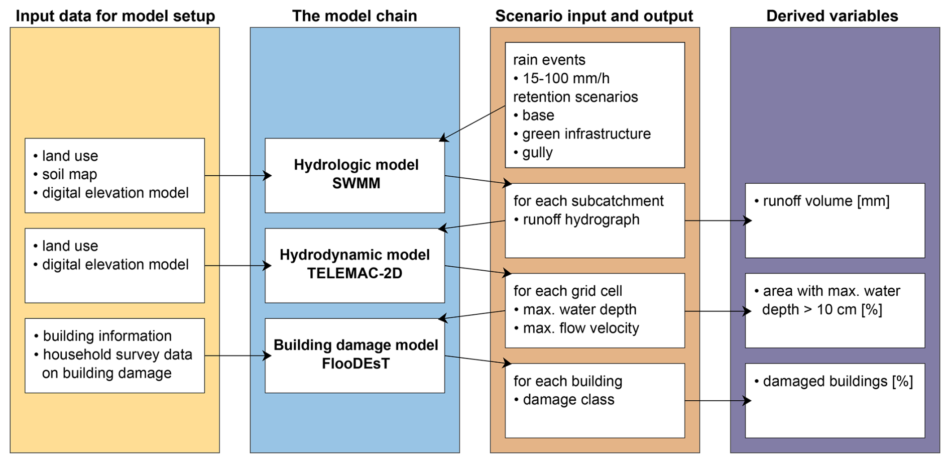
Figure 1 Workflow of data for model setup, scenario input and output through the model chain and derived variables.

2 Materials and methods

2.1 Workflow and data

The workflow of this study (Fig. 1) is based on three different models, which are executed consecutively: Storm Water Management Model (SWMM; EPA, 2023) is used for the hydrologic modelling, TELEMAC-2D (EDF, 2022) for hydrodynamics and Flood Damage Estimation Tool (FlooDEsT; Samprogna Mohor et al., 2025) for the building damage estimation.

These models require different input data. For the first two models, a land use map (vector shapefile; ALKIS, 2024) and a digital elevation model (DEM, 1 m × 1 m; ATKIS, 2024) were used. SWMM additionally needs a soil map (250 m× 250 m; Ross et al., 2018). The training data for the model FlooDEsT result from household surveys on building damage caused by past pluvial flood events. In its application, FlooDEsT uses building information from cadastral data (OpenStreetMap contributors, 2024) as input. Additionally, missing building information is imputed from the existing survey data distributions. For details on preprocessing of the input data, see Sect. 2.4.

To start the model chain, a combination of a specific synthetic rain event and retention scenario is defined. This serves as input for SWMM, which then produces a runoff hydrograph for each subcatchment, located at the subcatchment centroids. This, in turn, is the scenario input for TELEMAC-2D, which spatially simulates maximum water depth and maximum flow velocity. These are used by FlooDEsT to model the damage class of each building.

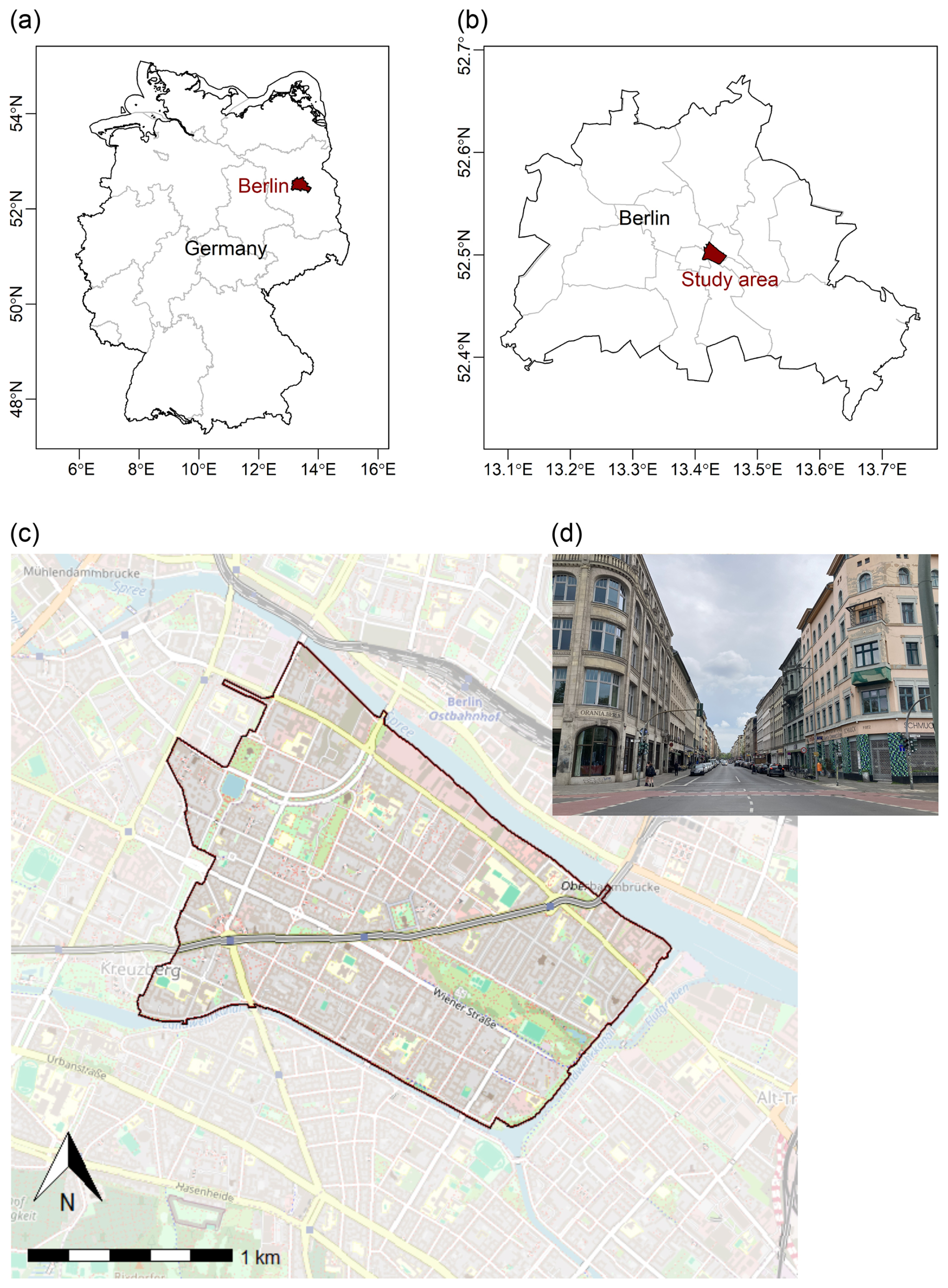
Figure 2 Study area location in Friedrichshain/Kreuzberg, Berlin: (a) Berlin in Germany; (b) location of the study area in Berlin; (c) land cover (©OpenStreetMap contributors, 2025, distribution under ODbL license); (d) typical street in the study area.

2.2 Study area

The study area (Fig. 2) is located in Berlin, i.e. in the district Friedrichshain-Kreuzberg/Mitte. With an area of 3.3 km² it is a small, very flat (heights in DEM ranging from 32–45 $\mathrm{m}\mathrm{a}.\mathrm{s}.\mathrm{l}.$) and highly sealed catchment, struggling with CSO. The study area is defined by the sewage system subcatchment and is bounded by the river Spree in the northeast and by the canal Landwehrkanal in the south and east. 30 % of the catchment is covered by buildings, 25 % with roads and 9 % with parks, playgrounds and sports fields.

The climate in Berlin is classified according to the Köppen–Geiger classification as warm temperate with precipitation throughout the year and warm summers (Kottek et al., 2006). The mean annual precipitation (MAP) is 577.7 mm and monthly means range from 28.5 mm in April to 77.5 mm in July. The mean annual temperature is 10.4 °C, with monthly means ranging from 1.3 °C in January to 20.0 °C in July (DWD, 2023, weather station Berlin Mitte, reference period 1991–2020).

2.3 Scenario definition

2.3.1 Rainfall events

The German National Meteorological Service (DWD) provides with KOSTRA 2020 (DWD, 2020a) a German-wide grid (5 km × 5 km) of statistical heavy rain events with different durations (5 min to 7 d) and return periods (1–100 years), based on the period 1951–2020. Recently, the German Federal Agency for Cartography and Geodesy has released maps of simulated inundation (depth, extent, flow velocity) as a response to two heavy rainfall scenarios (one with a return period of 100 years and one extreme scenario of 100 mm h⁻¹), applying a simplified hydraulic methodology (BKG, 2025). However, it is important to be aware that those simulations ignore any storm runoff reduction or retention, e.g. due to inflow into the urban drainage system (gully inflow) or due to infiltration into unsealed surfaces, such as parks, green areas, green infrastructure or pervious sealing. That means, these maps show effects of urban surface hydraulics only, but not for hydrological processes, such as infiltration or urban water retention.

In order to cover a wide range of heavy rain intensities (Table 1), this study includes synthetic rain events with a duration of one hour, based on the KOSTRA 2020 return periods of 1, 5, 10, 20, 50 and 100 years. As the study area is located in KOSTRA tile number 105190, this corresponds to rain totals of 14.8–48.9 mm for the investigated return periods (DWD, 2020b). Additionally, as suggested by BKG (2025), an extreme event with a rain total of 100 mm was included.

Table 1 Event total and maximum 5 min intensity of the investigated rain scenarios: KOSTRA events with return periods of 1–100 years and an additional extreme scenario, all with a duration of 1 h and Euler-II temporal distribution.

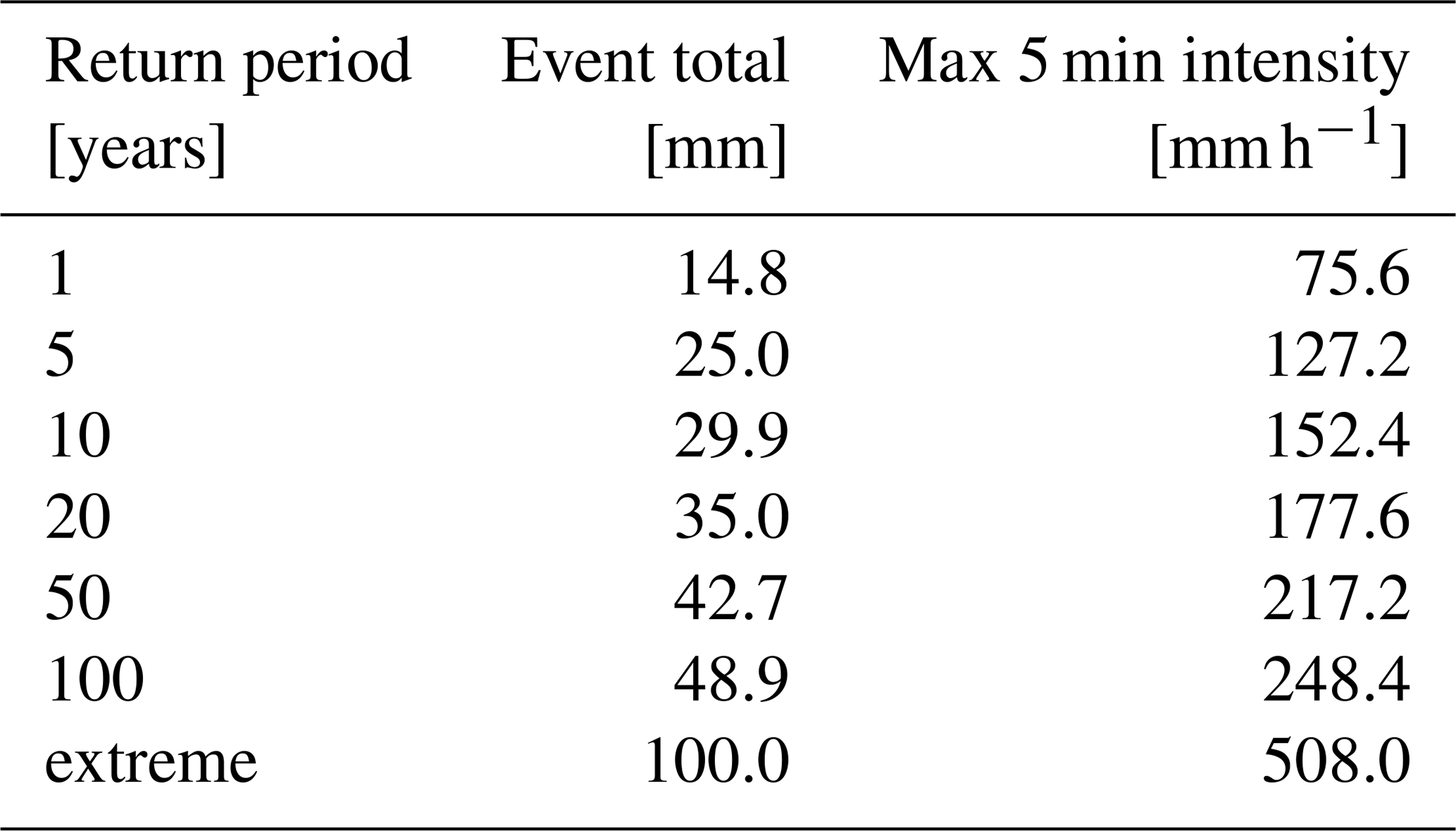
The temporal resolution of the synthetic rain events is 5 min, following Euler-II distribution, as it is established in Germany for the design of drainage systems (DWA, 2021). For example, the 100 year event has a rain total of 48.9 mm, with the following 12 consecutive 5 min rain totals: 3.3, 4.5, 7.4, 20.7, 2.3, 2.3, 1.6, 1.6, 1.6, 1.2, 1.2 and 1.2 mm. The maximum 5 min intensity of the selected rain events ranges from 75.6 to 248.4 mm h⁻¹ for the KOSTRA events, for the extreme event it is 508.0 mm h⁻¹.

2.3.2 Conventional stormwater management

The conventional stormwater management scenario (hereafter “gully” scenario) is designed following the recommendations for drainage systems of DIN EN 752-2. Here, the capacity of drainage systems in urban or residential areas is designed to fully meet a precipitation event with a return period of 5 years and a duration of 15 min. As our study area is located in the highly urbanised city centre of Berlin, we define gullies with a corresponding inflow capacity of 16 mm at the beginning of the rain event on all roads in the study area.

This simplification does not allow to represent processes such as sewer overflow to the surface. We opted for this approach nevertheless, as the detailed sewer network of our study area is not publicly available and the sewer system is not the focus of this study.

2.3.3 Green infrastructure

The assessed GI scenarios consist of single and combined GI measures, including three types of infiltration-based GI (see Dobkowitz et al. (2025) for more details on the GI measures):

• Bioretention system (BR): A shallow depression that collects surface runoff from surrounding impervious areas. The soil layer is covered with plants over a storage layer made of sand or gravel to obtain an elevated hydraulic conductivity. Optionally, at the bottom, there is an underdrain to the sewer system. BRs help to reduce runoff and remove pollutants.

• Green roof (GR): A greened soil layer over a drainage mat on top of a building, allowing the retention and evapotranspiration of water on roofs with inclinations of up to 45°. We can distinguish between extensive GR with a soil layer thickness of a few centimetres and intensive GR with a soil layer of at least 12 cm.

• Pervious pavement (PP): The pavement layer can be made of either impermeable paving blocks with permeable gaps filled with substrate, possibly with grass growing in them, or a pavement layer which is porous itself. Below, there is a storage layer with an optional underdrain, like for the BR. PP can be used for roads, sidewalks, squares and parking spaces.

For the maximum GI scenarios, potential GI extents were defined as follows: BR on 10 % of the study area, including roads and residential subcatchments after subtracting the area covered by buildings (BR_max), GR on all buildings (GR_max) and PP on 50 % of the roads (PP_max). Based on these definitions, the medium GI scenarios were defined as half of the maximum extents (BR_med, GR_med and PP_med). Additionally, two combined scenarios were defined, GR_max + PP_med and BR_max + GR_max. For both of them, GR_max was combined with one of the other GI types because there is no spatial overlap between them.

Table 2 Retention scenarios: definition, impervious (roads, buildings), pervious (backyards, parks) and green infrastructure (GI) covered areas. Except for the gully scenario, the drainage system was not considered.

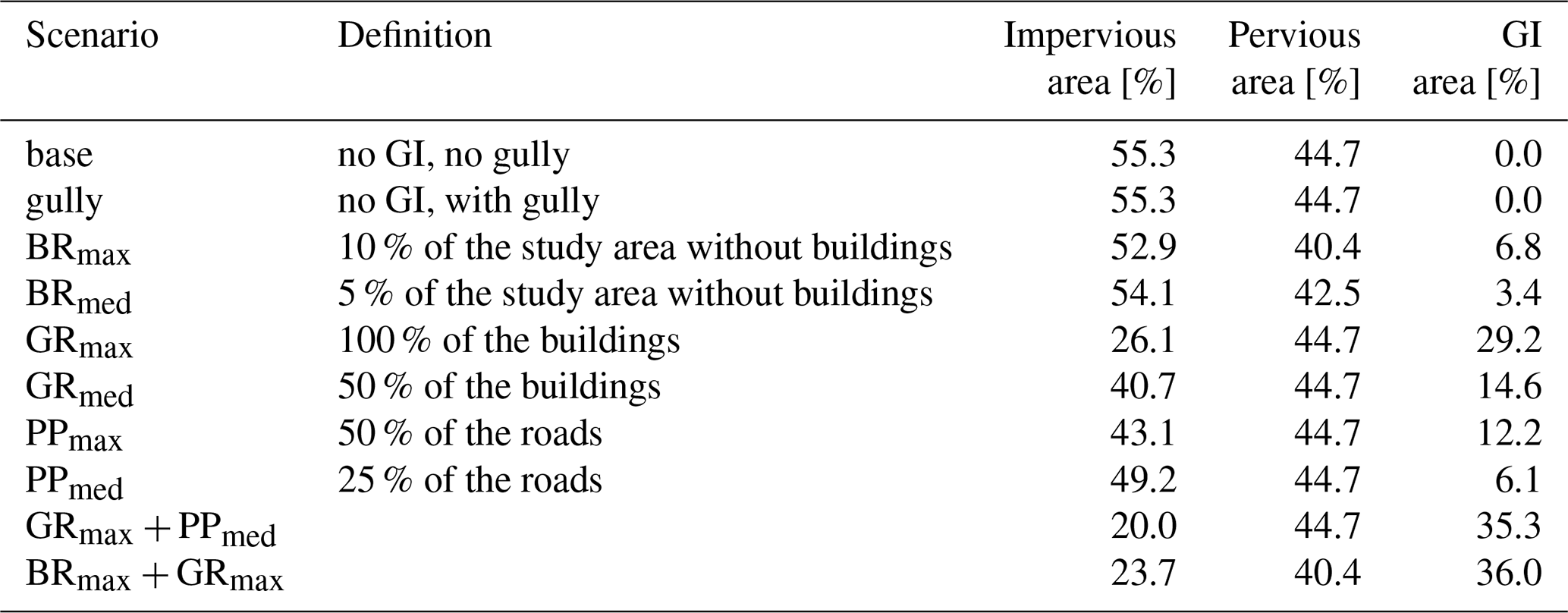
Table 2 provides an overview of the retention scenario definitions and the respective percentage of the study area that is impervious, pervious or covered by GI. The base and gully scenarios include no GI, with an impervious area of 55.3 % and a pervious area of 44.7 %. For the GI scenarios, the GI area is subtracted from the impervious and/or pervious areas, resulting in impervious areas ranging from 20.0 %–54.1 %, pervious areas of 40.4 %–44.7 % and GI areas of 3.4 %–36.0 %.

Table 3 Bioretention system (BR), green roof (GR) and pervious pavement (PP) layer characteristics and usage. If no other source is indicated, the parameters were defined according to the EPA SWMM 5.2 User Guide (EPA, 2023).

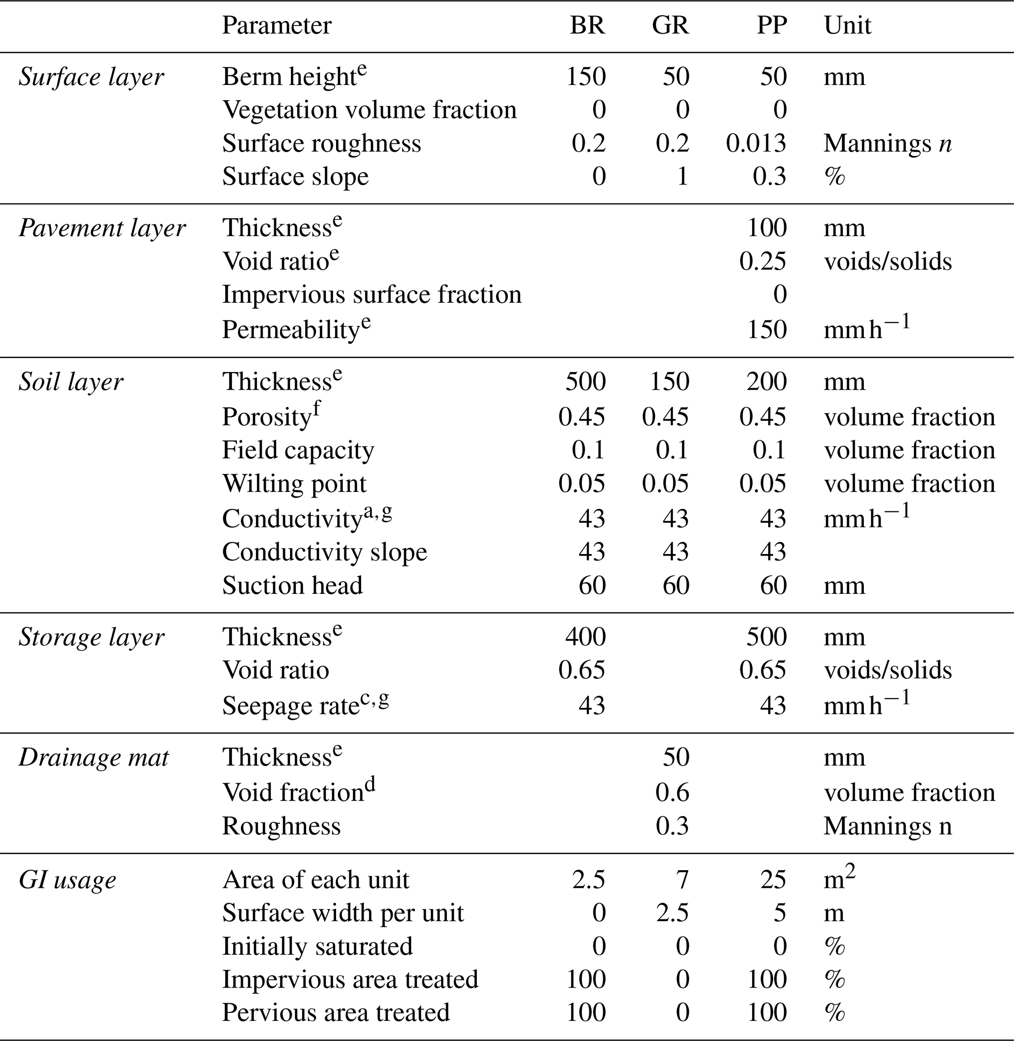
^a Conductivity: saturated hydraulic conductivity. ^b Conductivity slope: calculated from soil type with the equation from EPA (2023): $\mathrm{0.48}\times \text{sand}\left[\mathit{\%}\right]+\mathrm{0.85}\times \text{clay}\left[\mathit{\%}\right]=\mathrm{0.48}\times \mathrm{80}+\mathrm{0.85}\times \mathrm{5}=\mathrm{43}$. ^c Seepage rate: rate at which water seeps into the native soil below the layer. ^d Void fraction: ratio of void volume to total volume in the mat. ^e Dobkowitz et al. (2025), ^f Rossman and Bernagros (2018), ^g Schaap et al. (2001).

The GI types BR, GR and PP are implemented in SWMM as “LID Controls”, i.e., “Bio-Retention Cell”, “Green Roof” and “Permeable Pavement”. For the required input parameters, we extracted typical design parameters and soil hydraulic parameters from Dobkowitz et al. (2025); EPA (2023); Rossman and Bernagros (2018); Schaap et al. (2001). As loamy sand is common in Berlin, we used the soil hydraulic parameters from this soil type. Table 3 shows the resulting set of parameters.

The unit area of a certain GI type is replicated within each subcatchment until reaching the defined spatial extent. In the case of GR and PP, the surface width per unit is used to define how the overland flow leaves the GI unit. For BR, instead, the surface width is zero as the runoff just spills over the berm. BR and PP receive all runoff from impervious and pervious areas of the same subcatchment, while GR can receive only the direct rainfall.

2.4 The model chain

2.4.1 The hydrologic model

The rainfall-runoff modelling was conducted using the dynamic hydrologic-hydraulic model SWMM. For runoff simulation, the study area was divided into subcatchments, each with its own pervious and impervious fraction (Rossman, 2010). Evapotranspiration was not included, as it is negligible when considering single events.

Based on the land use dataset, the study area was divided into 230 subcatchments, with two subcatchment types: roads, covering 25 % of the study area, and residential, covering the remaining 75 %. The residential subcatchments summarise building blocks, including backyards and parks, instead of considering each building separately. The subcatchments' average slope was calculated from the DEM.

For infiltration, the SCS-Curve Number (CN) method (Mishra and Singh, 2003) was used. CNs for each subcatchment were assigned by combining the land use dataset with the soil map, resulting in CNs ranging from 61–98, with an area-weighted mean CN of 91 (Fig. 3). A higher CN indicates higher impermeability and less infiltration.

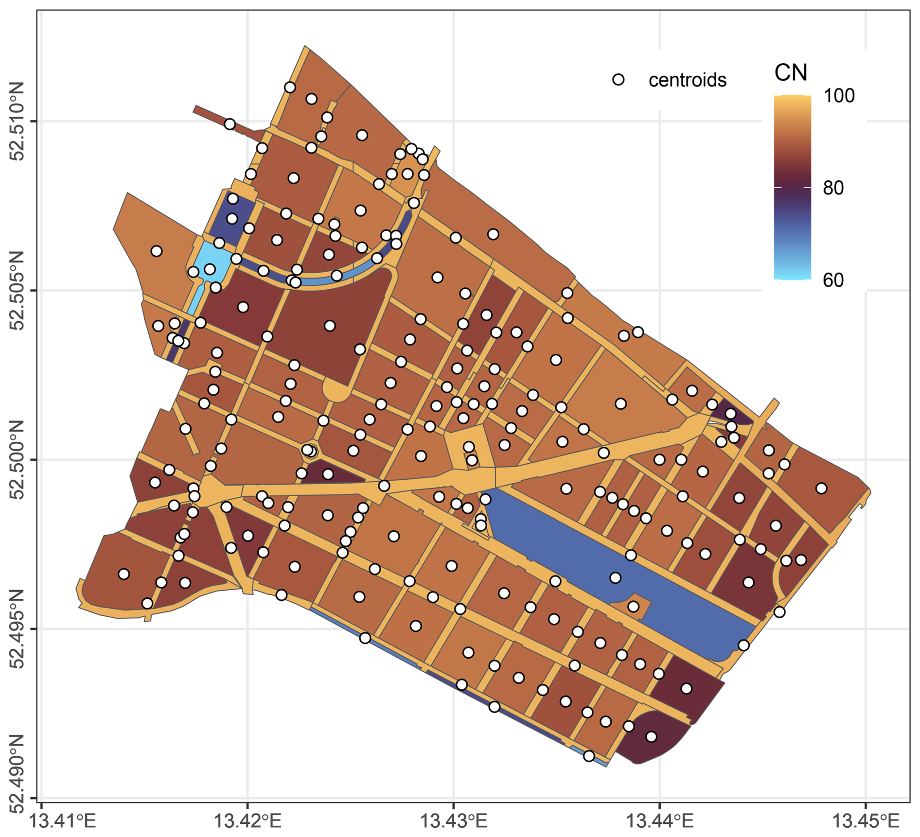
Figure 3 Subcatchments with their SCS-Curve Numbers and centroids, which are the outlet points in SWMM and single nodal inflows in TELEMAC-2D.

Different from the remaining study area, the GI modules use the Green-Ampt method. For each subcatchment, the runoff generated by the impervious area is routed to the pervious area, and what remains is routed to the GI, when there is BR or PP. As the sewer system is not publicly available, the gully water absorption was represented by increasing the depression storage of the roads.

From the simulation results, the runoff hydrographs for each subcatchment were forwarded as input to the hydrodynamic model for subsequent modelling of the surface flood dynamics.

2.4.2 The hydrodynamic model

For the hydrodynamic simulations, the open source TELEMAC system is used. TELEMAC incorporates a 2D module that applies a finite element scheme with a semi-implicit solver on a triangulated mesh to solve the Shallow Water Equations (EDF, 2022).

The hydrodynamic model has an unstructured mesh with a resolution of 2 m which results in a total of approximately 768 000 nodes and 1 458 000 elements. Buildings are represented as holes in the model. The roughness coefficients are derived from the land use data using the guidelines from LUBW (2020). The topography is interpolated from the DEM.

The output hydrographs from the hydrologic model are represented in the hydrodynamic model by single nodal inflows and serve as the only input into the hydrodynamic model. The river Spree and the Landwehrkanal are used as outlet boundary conditions in the northeast and south and east, respectively. The northwest boundary in the hydrodynamic model is moved outward compared to the hydrologic model to generate a less undulating model boundary line, which facilitates defining the boundary conditions here. The northwest boundary is defined as a closed wall, which prohibits water from leaving through this boundary, but does not create extensive backwater effects into the study area, as the model is spatially extended at this boundary. A more detailed description of the hydrodynamic model and the validation of the boundary conditions is provided in De Vos et al. (2024).

The maximum water depths and velocities are extracted from the simulation results and rastered with a 1 m × 1 m resolution. These rasters are then forwarded to the building damage model.

2.4.3 The building damage model

In order to further assess the potential benefits of the GI measures, a building damage model was used. Despite the existence of numerous models to estimate flood damage to buildings, most were developed for typical riverine floods, whilst research has shown that different flood pathways show different damage patterns (Mohor et al., 2021; Gerl et al., 2016). Therefore, the “Flood Damage Estimation Tool” (FlooDEsT; Samprogna Mohor et al., 2025) was adopted as it was specifically developed for urban pluvial floods.

The model is based on survey data from past urban pluvial flood events between 2010 and 2016 in Germany (see Thieken et al., 2017). However, the survey data provides no data points from our study area. The survey data were split for training and testing. Using a recursive partitioning algorithm, the XGBoost (Chen and Guestrin, 2016), the model generates an additive ensemble of decision trees, where sequential trees are trained to correct the residual errors made by previous ones. The recursive partitioning algorithm is powerful at capturing non-linear relationships between the predictors (hazard characteristics, building characteristics) and the outcome variable (relative building damage). The input variables are a mix of physical and conceptual variables: water depth [m], flood intensity (in form of classes of people stability in flood waters), the presence of contaminants in the water, building area, building age, presence of a basement, and implemented adaptation measures in form of a score. For a detailed description of the input variables, especially how scores are calculated, consult Thieken et al. (2005).

After the random sampling process, despite some variation in the estimated damage degree, in 97 % of the runs the estimations fell under the same damage class, which indicates great stability of results. The model calibration performed well with a RMSE of relative building damage of 0.03 with the training data and 0.06 with the test data after 7 boosting rounds (i.e. additive trees). Relative building damage is the ratio between repair or replacement costs and the building value. Hence, 0.06 means a 6 % relative damage.

In the application, the model needs the maximum water depth and flow velocity from the hydraulic model (from which flood intensity is derived) and building information from cadastral data (either authoritative or OpenStreetMap data). Maximum water depth and flow velocity do not necessarily occur at the same time, and this is a potential bias in our approach, in which we potentially overestimate the hazard. We do so for a compatibility of approaches with other data sources, namely (official) flood hazard maps, which often provide solely the maximum water depth and flow velocity of a scenario. The same occurs in the survey data used for training, where only maximum water depth and maximum “intensity” are reported.

Additionally, the tool uses smart random sampling to impute missing variables, such as building-level features, from the existing survey data distribution, which secures representativeness of buildings affected by this flood pathway, reducing exposure bias. Regardless of property size or market value, damage classes based on relative damage are provided, facilitating comparison. The damage classes are defined as follows: Low = 0 %–5 %, Medium = 5 %–10 %, High = 10 %–15 %, Very high = 15 %–100 % relative damage.

2.5 Evaluating the flood mitigation impact of the retention scenarios

Combining all rain and retention scenarios described in Sect. 2.3, in total 70 scenarios were defined. After processing them through the model chain, the flood mitigation impact of the GI scenarios was assessed using the following variables: runoff total from the hydrologic model, percentage of the study area with maximum water depth > 10 cm from the hydrodynamic model and the percentage of damaged buildings (see Fig. 1).

In order to assess the flood mitigation impact comprehensively, from each of these variables, the following three indices were calculated: First, the absolute reduction compared to the base scenario (Eq. 1), second, the relative reduction (as percentage, Eq. 2) and third, the absolute reduction per square meter of GI (Eq. 3), with X for the respective variable, such as runoff total or percentage of damaged buildings. X_base represents the base scenario, X_scen the considered retention scenario. For the gully scenarios, only Eqs. (1) and (2) can be applied, as no spatial extent was assigned to the gullies.

$$\begin{array}{}\text{(1)}& {\displaystyle }& {\displaystyle }{\mathrm{Red}}_{\mathrm{abs}}=X_{\text{base}}-X_{\text{scen}}\text{(2)}& {\displaystyle }& {\displaystyle }{\mathrm{Red}}_{\mathrm{rel}}={\displaystyle \frac{X_{\text{base}}-X_{\text{scen}}}{X_{\text{base}}}}\cdot \mathrm{100}\text{(3)}& {\displaystyle }& {\displaystyle }{\mathrm{Red}}_{\mathrm{abs},\mathrm{GI}}={\displaystyle \frac{X_{\text{base}}-X_{\text{scen}}}{G{I}_{\text{share}}}}\end{array}$$

In the literature, relative reduction is the most common index. However, it gives a large emphasis on the flood reduction of small rainfall events. Absolute reduction was added to see the actual retention of the scenarios, using the same unit as the considered variable. Regarding this index, the possible range is limited by small values of the considered variables for the smaller rain events. Additionally, the GI implementation degree influences a lot the result. Therefore, absolute retention per square meter of GI was included as well.

Flow velocity in combination with water depth is crucial for damage modelling. However, due to the flat topography of the study area, flow velocities are rather low. Hence, flow velocity was not discussed separately in the flood mitigation analysis.

3 Results

This section begins with the results of the hydrologic, hydrodynamic and building damage models. Then, flood mitigation is evaluated according to the absolute reduction, relative reduction and, finally, regarding the spatial efficiency of the studied GI types.

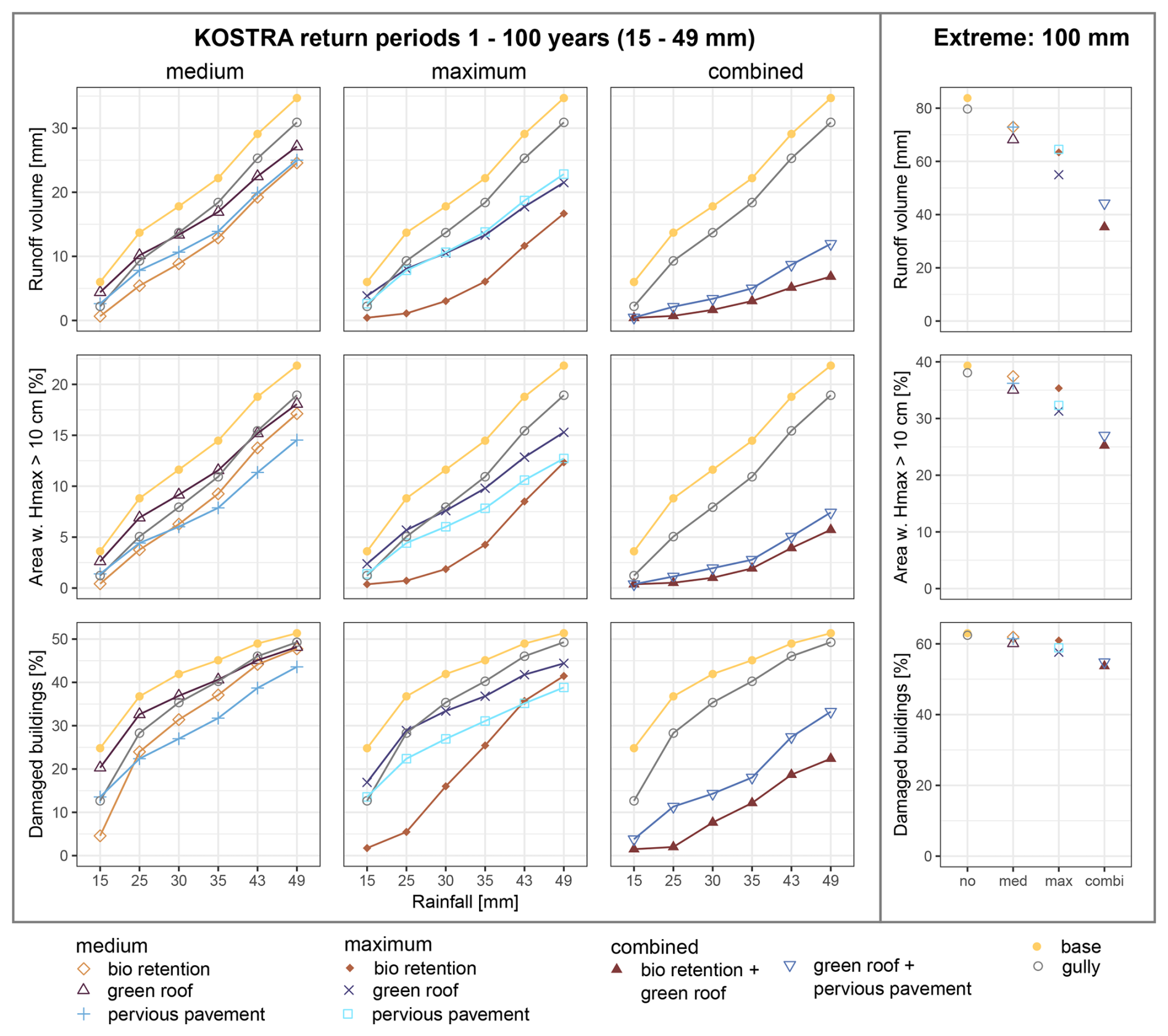
Figure 4 Results of the model chain: runoff total, area with maximum water depth (Hmax) over 10 cm and percentage of damaged buildings for six rain events (KOSTRA return periods 1, 5, 10, 20, 50, 100 years and an extreme event with 100 mm), comparing base and gully scenario to the medium, maximum and combined GI scenarios.

3.1 Pluvial flood response through the model chain

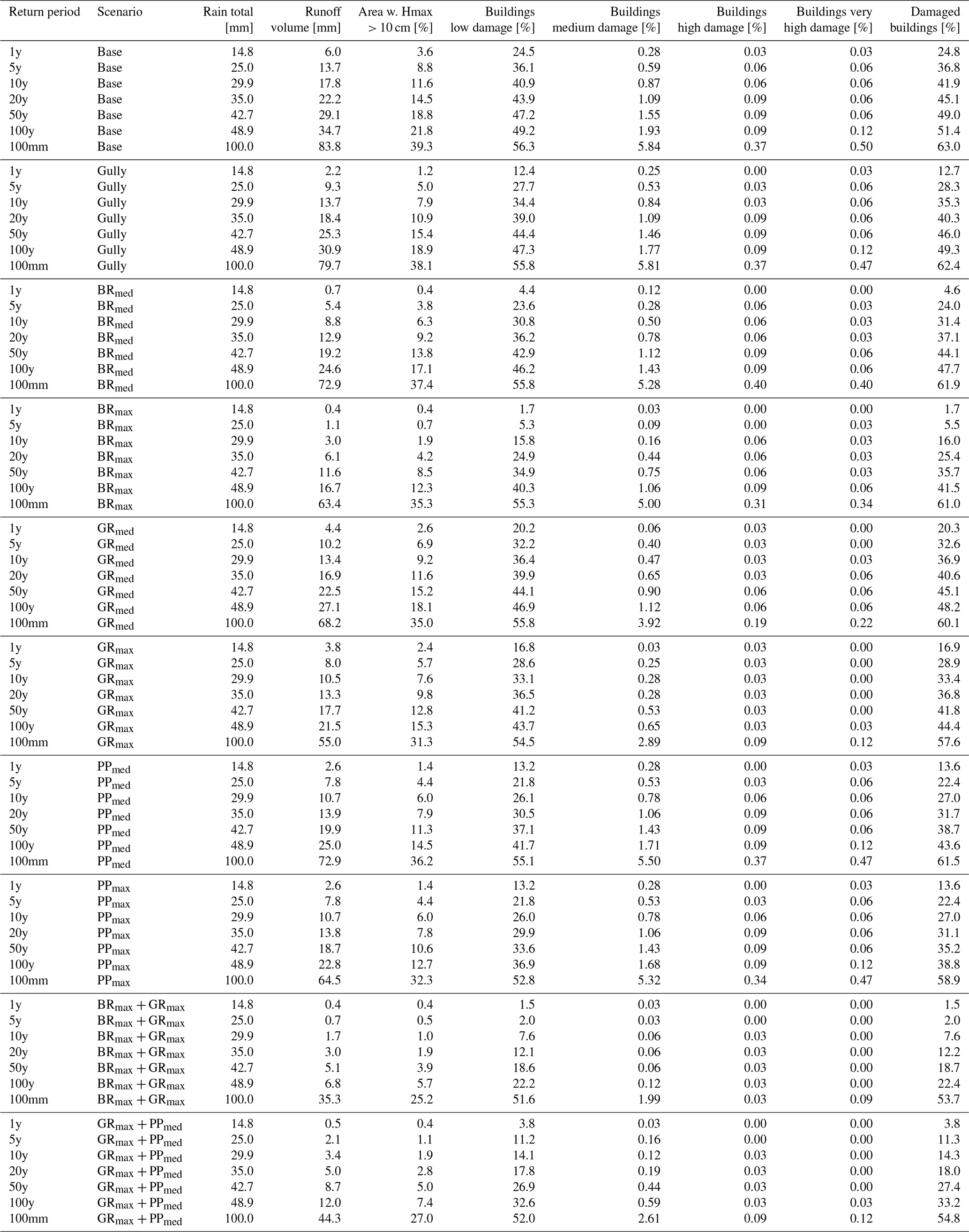
Figure 4 gives an overview of the results of the model chain, showing event runoff [mm] (first row), the percentage of the study area with a maximum water depth > 10 cm (second row) and the percentage of damaged buildings for the different rainfall and retention scenarios (third row), see also Table A1.

Referring to the rainfall scenarios, the first three columns of Fig. 4 show the KOSTRA events, with the medium retention scenarios in the first, the maximum retention scenarios in the second and the combined retention scenarios in the third column. For a better visibility of the KOSTRA events, the extreme event with a rain total of 100 mm was plotted with a different y-axis separately in the fourth column. The base and gully scenarios are shown in all columns to improve comparability.

In general, all retention scenarios show less runoff, flooded area and building damage than the base scenario. The maximum GI scenarios outperform the medium GI scenarios and the combined scenarios outperform all single GI scenarios.

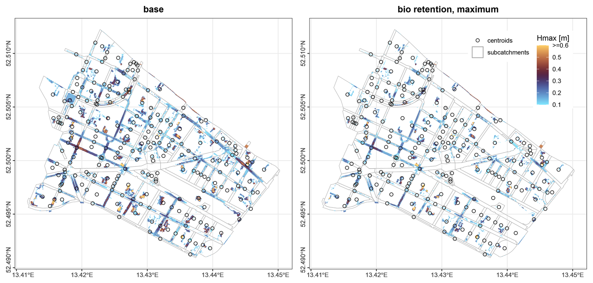
Figure 5 Spatial results of the hydrodynamic model: area with maximum water depth (Hmax) > 10 cm and its depth for the 49 mm rain event (KOSTRA return period 100 years), comparing base and maximum bioretention scenario.

Figure 5 shows the spatial distribution of the maximum water depth for two exemplary scenarios. It illustrates that BR_max reduces flood extent and maximum water depth compared to the base scenario.

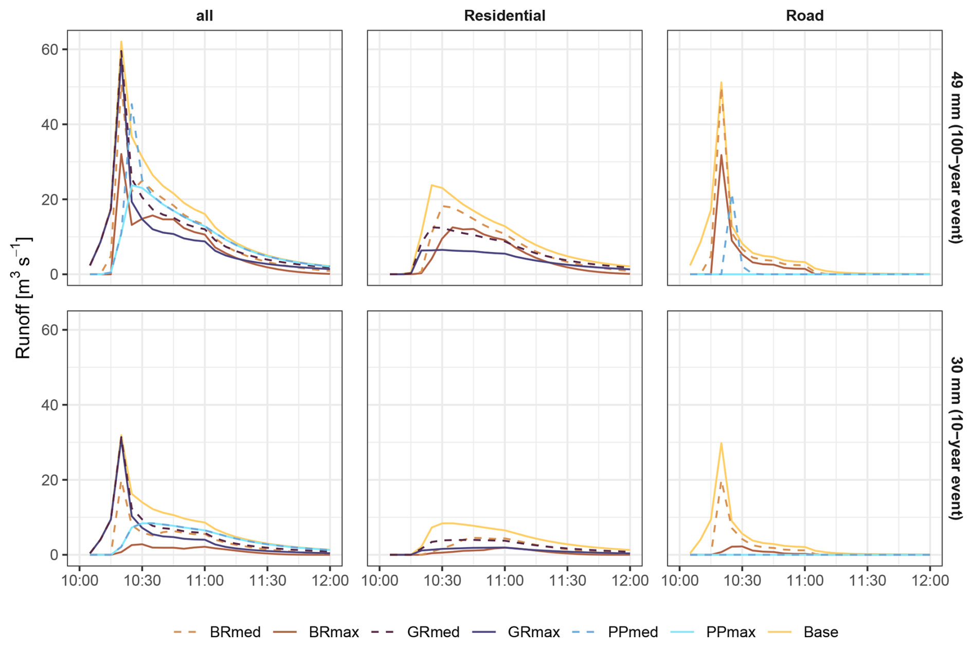
Figure 6 Runoff hydrographs summarized for the entire study area (left column), residential (middle) and road (right) subcatchments for two rain events (KOSTRA return periods 10 and 100 years), comparing the runoff of the base scenario to the single GI scenarios. The residential hydrographs of PP_med and PP_max and also the road hydrographs of GR_med and GR_max are equal to the base scenario.

Among the single GI scenarios, BR produces the lowest runoff with medium and maximum extent. Regarding the flooded area and damaged buildings, BR_max is also the strongest among the single GI scenarios with maximum extent, however, at the medium scenarios, PP_med outperforms BR_med in most events. This can be explained by a look at the temporal distribution of runoff. Figure 6 shows the runoff hydrographs for the base and single GI scenarios for two exemplary rain events. In the first column, all subcatchments are included, in the second column only runoff from residential subcatchments and in the third column only runoff from road subcatchments is summarized. It shows clearly how much higher the peak runoff and shorter the runoff duration is for road subcatchments without GI measures compared to the residential subcatchments. In both represented rain scenarios, the overall peak runoff for BR_med is more than twice than for PP_med. This results in a larger flooded area and more damaged buildings for BR_med, although the runoff volume is lower compared to PP_med.

The gully scenario shows the lowest flood mitigation impact, only for the 1 year event it outperforms GR and PP, and among the medium scenarios, it outperforms GR at the flooded area and damaged buildings for several of the smaller events.

The combined scenario GR_max + BR_max provides the highest flood mitigation. Regarding the 49 mm event, it reduces the runoff and area with flood depth > 10 cm to values below the 25 mm base scenario. The damaged buildings drop even below the 15 mm base scenario.

In the following sections, we will look at the flood mitigation impact indices defined in Sect. 2.5 for a more comprehensive performance evaluation.

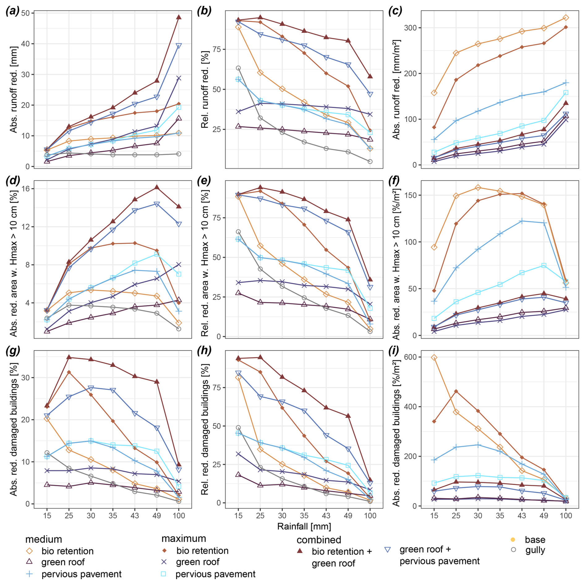
Figure 7 Absolute (a, d, and g) and relative (b, e, and h) flood mitigation and spatial efficiency (c, f, and i) of the assessed rainfall and retention scenarios: runoff total (a–c), area with maximum water depth (Hmax) > 10 cm (d–f) and percentage of damaged buildings (g–i).

3.2 Absolute flood reduction

Absolute flood reduction (Fig. 7a, d, g) is in most rain scenarios the highest for the combined GI scenarios. However, in some events, they are partially outperformed by other retention scenarios. For example, BR_max is among the scenarios with the highest reductions for the smaller events, for the larger events, its impact decreases. With increasing event rainfall, we observe a decrease in the reduction of damaged buildings. The low damage class constitutes in all scenarios the largest share of the total number of damaged buildings.

3.3 Relative flood reduction

Relative flood reduction (Fig. 7b, e, h) results in a reduction of runoff total by 4.9 %–94.8 %. The flooded area with maximum water depth > 10 cm is reduced by 3.2 %–94.1 %. Building damage is reduced by 0.9 %–94.6 %, with 0.8 %–94.6 % in the low, 0.0 %–96.0 % in the medium, −8.3 %–100 % in the high and 0.0 %–100.0 % in the very high damage class.

For most retention scenarios and variables, relative flood reduction decreases clearly with increasing rainfall, only for the GR scenarios (GR_med and GR_max) this trend is less apparent. For most events and variables, the combined scenarios and BR_max show the strongest results. The gully scenarios show a medium performance for the 1 year event and then decrease with increasing event rainfall to quite small absolute and relative flood reduction values compared to the GI retention scenarios.

3.4 Spatial efficiency of the different green infrastructure types

Absolute flood reduction per square meter of GI (Fig. 7c, f, i) allows to compare the spatial efficiency of the different GI scenarios. Regarding runoff, the reduction per square meter increases with increasing rainfall and BR_med shows at each event the highest reduction, followed by BR_max and PP_med. Area with maximum water depth > 10 cm first increases and after a peak at the events with 30–43 mm decreases with increasing event total. Again, BR_med, BR_max and PP_med achieve the highest reduction per square meter. Only at the 100 mm event, PP_max outperforms BR_med, BR_max and PP_med. The building damage reduction is the smallest for the 100 mm event.

4 Discussion

4.1 Green infrastructure scenarios – realistic or too ambitious?

The results of our study show that, with an intense implementation of GI, high absolute and relative flood mitigation can be achieved. However, retrofitting GI in a historically grown city is much more challenging then designing GI for a fully new housing development.

To address the question of how realistic the implementation of the different investigated GI scenarios is in practice, we compare our scenarios to those elaborated by Knoche et al. (2024). They conducted workshops with the Senate Department for Urban Mobility, Transport, Climate Protection and the Environment (SenMVKU), the Berlin water supply and drainage company (Berliner Wasserbetriebe; BWB), the Berlin rainwater agency (Berliner Regenwasseragentur) and two Berlin district authorities in order to define realistic stormwater management strategies. These scenarios included different types of GI, such as green roofs and unsealing of parking spaces, to achieve a reduction of sewage overflows in the area of Berlin drained by a combined sewer system.

Within a timeframe of 10 years, Knoche et al. (2024) suggest an unsealing of 5.5 % of the study area, with 1.5 % located on streets and 4 % on properties. Accordingly, both BR scenarios are realistic to be implemented within the next 10 years.

Within 30 years, an unsealing of 27.5 % is suggested, with 4.5 % on streets and 22.5 % on properties. This means that GR_med is realistic within the next 30 years. The scenarios PP_med and PP_max, however, require with 25 % and 50 % a much higher unsealing of streets. Besides, the 3 scenarios with the largest conversion to GI (GR_max, GR_max + PP_med and BR_max + GR_max) require reductions of impervious area beyond those elaborated by Knoche et al. (2024) for a timeframe of 30 years. Hence, their realisation within the next decades seems unrealistic.

Besides the spatial extents of the GI scenarios, flood mitigation is sensitive to design parameters such as berm height and layer thickness, and their hydraulic parameters. These parameters were selected based on the literature as described in Sect. 2.3.3 and we did not include more variations of each GI type, as the focus of this study is the comparison between different rain events and the propagation of the flood mitigation through the model chain. However, testing more parameter sets would allow to investigate if the comparison of different GI types is robust or too sensitive to the parameters.

4.2 Space efficiency versus continuation of former land use

As shown in this study, BR is the GI measure that provides the highest flood mitigation per square meter. Nevertheless, when we discuss space efficiency, we also need to take into account whether the GI implementation impedes other uses of the space. In the case of GR, the usability of the building does not change. For PP, at least parking spaces and residential roads with reduced speed and traffic load continue providing the same functionality. In contrast, BR requires the surface area to be free from buildings and traffic. Still, GI can provide further ecosystem services beyond flood mitigation by increasing groundwater recharge (Bhaskar et al., 2018) and, if a vegetation cover is present, contribute to the mitigation of urban heat stress (Cristiano et al., 2022; Watrin et al., 2019) through evapotranspirative cooling, increase biodiversity (Monberg et al., 2018) and improve the aesthetic value of the urban environment.

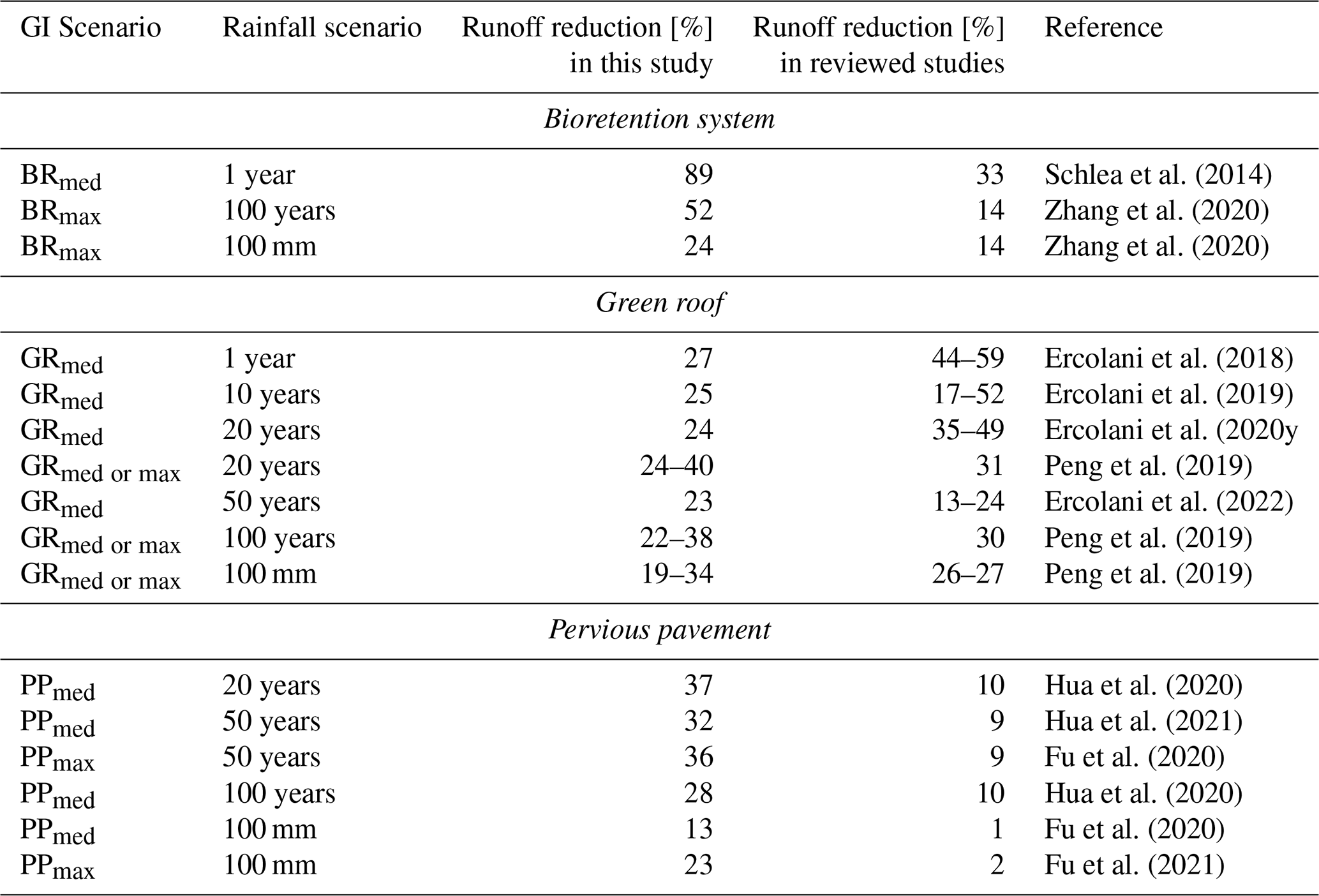
Table 4 Comparison of relative runoff reduction with other studies.

4.3 Comparison of the simulated flood mitigation to previous studies

Due to the nature of a scenario analysis, there are no measurement data for validating the flood mitigation impact of the GI scenarios modelled in this study. Instead, we can compare our results to data from the literature. As surface runoff is the most directly affected by the GI measures, we will focus on this variable in the following section. Nevertheless, surface flooding and building damage will also be considered.

4.3.1 Runoff retention

In order to compare the GI impact on runoff volume with other studies, we selected examples from those studies reviewed in Dobkowitz et al. (2025) based on similarity of study area, event and retention scenario characteristics. More specifically, we considered only events with a duration of 0.5–2 h and rain totals of 10–60 mm and 90–110 mm, as the rain totals modelled in our study range from 15–49 mm and 100 mm was added as an extreme event. Regarding the area covered by GI, we selected those studies with 1 %–10 % of the study area for BR, with 10 %–45 % for GR and with 4 %–20 % for PP. Finally, the impervious area for selecting a study was restricted to 20 %–50 % for GR and 15 %–70 % for PP. Due to the smaller amount of available studies, this last criterion was not applied when selecting BR studies. The selection resulted in 25 events from 6 studies, relative runoff reduction from these studies is shown in Table 4:

• Ercolani et al. (2018) used the model smart-green (MOBIDIC-U and a QGIS plugin) to investigate GR in a 1.9 km² study area in Milan, Italy (MAP 800 mm). The GR is composed of a 200 mm soil layer and a 150 mm drainage mat.

• Fu et al. (2020) coupled SWMM and Hydrus-1D to model PP in a 3.3 km² study area in Xiamen, China (MAP 1413 mm). Below the permeable brick layer with a thickness of 60 mm, there are 4 different permeable layers with in total 940 mm.

• Hua et al. (2020) studied PP, using the model MIKE URBAN for a 7.4 km² study area in Chaohu, China (MAP 1307 mm). In this study, the pavement layer thickness is 120–180 mm, underlain by 300 mm of permeable material.

• Peng et al. (2019) investigated GR with SWMM in a 0.044 km² study area in Fuzhou, China (MAP 1500 mm). The GR has a berm height of 15 mm, a soil layer thickness of 150 mm and a drainage mat of 30 mm.

• Schlea et al. (2014) investigated BR with an experimental study, using a rain gauge, graduaded containers for runoff and drainage measurements and piezometers for water table changes. This setup was used in a 869 m² study area located in Westerville, USA (MAP 1105 mm). The layer thicknesses were not reported in the study.

• Zhang et al. (2020) modelled BR with SWMM in a 6.07 km² study area in Kyoto, Japan (MAP 1677 mm). The BR has a berm height of 150 mm, soil layer thickness of 700 mm and a storage layer of 300 mm.

Regarding BR, relative runoff reduction in the reviewed studies is 44 %–73 % lower than in our study. A possible explanation for this difference is that the impervious area is 46 %–75 % higher in these studies. This increases runoff formation in the remaining study area and reduces the relative runoff reduction of BR. The BR extent of the event from Schlea et al. (2014) is 38 % lower than in our study, which also decreases the runoff retention. However, for the two compared events from Zhang et al. (2020), the BR extent shows no significant difference. Rain totals are with at most 15 % not significantly higher in the compared studies.

For GR, most of the examples from Ercolani et al. (2018) result in much higher runoff reduction. This can be a result of the 36 %–49 % lower imperviousness of the study area. In terms of the GR extent, Ercolani et al. (2018) has two settings, with GR covering 10.3 % or 15.4 % of the study area. In the first case, this is 29 % less GR then in the GR_med scenario and results in 43 % less to 64 % more runoff reduction. In the second case, this is 5 % more GR then in the GR_med scenario, resulting in 6 %–120 % more runoff reduction. Furthermore, the GR layers investigated by Ercolani et al. (2018) are more thick, which allows to retain more water.

With respect to the GR extent, the scenarios from Peng et al. (2019) are between GR_med and GR_max, i.e. the GR extent is 48 % larger than GR_med and 26 % smaller than GR_max. The imperviousness of the study area is closer to GR_med, as it is 22 % higher than GR_med and 91 % higher than GR_max. The runoff reduction from Peng et al. (2019) turns out to be centred between the runoff reduction of the corresponding scenarios, with 30 %–45 % more runoff reduction than GR_med and 21 %–24 % less runoff reduction than GR_max.

PP shows less runoff reduction in both reviewed studies. When comparing to Hua et al. (2020), the 63 %–72 % lower runoff reduction can be caused by the 42 % higher imperviousness of the study area compared to PP_med and 28 % smaller PP extent. However, with regard to Fu et al. (2020), the impervious area is 7 %–25 % smaller and the PP extent 9 %–63 % larger than in the corresponding scenarios of this study. Still, runoff retention is 75 %–92 % lower. This is even more surprising, as the saturated hydraulic conductivity of the different layers of the upper 35 cm is with 133–606 mm h⁻¹ much higher than in our study (43–150 mm h⁻¹, see Table 3). Only the plain fill below has with 10.2 mm h⁻¹ a lower conductivity.

4.3.2 Flood volume reduction

Neumann et al. (2024) and Tügel et al. (2025) investigated flood volume reduction by GI in Berlin. Neumann et al. (2024) studied the impact of extensive GR, intensive GR and GR with enhanced retention (retention roof), among other GI measures. They investigated the same study area as our study, using the software InfoWorksICM (Autodesk, 2023). Tügel et al. (2025) coupled the models hms⁺⁺ (Steffen and Hinkelmann, 2023) with SWMM and assessed the impact of retention roofs and gullies in a 13 km² study area in the centre of Berlin, with 35 % roof and 16 % road surfaces.

Despite the similarity of the study areas, GI extents and rain event characteristics, comparability is limited by the use of different measures of flood volume. While Neumann et al. (2024) defined flood volume as the sum of maximum water level in each mesh element with at least 10 cm water depth, Tügel et al. (2025) used the sum of maximum water level of all mesh elements. In our study, the percentage of the study area with a maximum water level > 10 cm is used. Besides, the reviewed GR scenarios and the reference base scenarios are combined with the sewer system in most cases, whereas our study uses GI and base scenarios without gullies.

Comparing relative flood reduction despite these limitations in comparability, we see that Neumann et al. (2024) reports the most similar results for the 100 year event, with a flood volume reduction of 32 % for extensive GR and 34 % for intensive GR and retention roofs. This is very close to GR_max with a 30 % reduced area with maximum water level > 10 cm.

For the 100 mm event, flood volume reduction according to Neumann et al. (2024) is 14 % for extensive GR and 34 % for intensive GR and retention roofs, while GR_max results in a reduction of the area with maximum water level > 10 cm of 20 %. It is noticeable that in the study of Neumann et al. (2024) there is hardly any difference in relative flood volume reduction between intensive GR and retention roofs regarding the 100 year and the 100 mm event, showing that the 100 year event does not make full use of the retention potential of those GR types.

Comparing the gully water retention to a base scenario without drainage system, Tügel et al. (2025) report a much larger impact of the drainage system than our study. For the 100 year event, Tügel et al. (2025) result in 31 % reduction of flood volume while our gully scenario results in 13 % less area with maximum water level > 10 cm. For the 100 mm rain event the relative difference still increases, with 26 % (Tügel et al., 2025) compared to 3 % from our gully scenario.

Possible explanations for the difference are the different study areas, different models and model parametrisations or the different implementation of the drainage system itself. While Tügel et al. (2025) used the drainage system model from BWB, which is a restricted dataset, in our study a simplified approach was used by defining gully water absorption due to the official drainage system requirements. Alternatively, a virtual drainage system based on open data could be created using the method presented by Montalvo et al. (2024). It depends on the use case, if the additional effort for the drainage model setup is worth for including a more complex drainage system in the model chain.

Furthermore, the discrepancy in the flood mitigation impact between the compared studies can be explained by the use of different measures of flood volume itself. Strong reductions at localized hotspots with very high maximum water depth could result in a disproportionate decrease of total flood volume compared to the area-based indicator used in this study.

4.3.3 Building damage mitigation

Staccione et al. (2024) tested the effect of GI (GR and green open spaces) on building damage reduction in Milan (Italy), considering progressive higher intensities of green conversion and different rainfall scenarios. Overall, it was found that GI can reduce flood impact, but proportionally, the higher gains occur for lower rain intensities. The 100 year event corresponds to 54.7 mm in 1 h. A 100 % implementation of GR potentially reduces building damage by ca. 21 % for the 100 year event (or ca. 39 % of the expected annual damage (EAD), integrating all rainfall scenarios), whilst a conversion of 50 % to GR reduces damage by ca. 17 % for the 100 year event (32 % reduction of EAD). In turn, a conversion of 25 % of potential green areas reduces building damage by ca. 13 % for the 100 year event (or 25 % reduction of EAD).

Our analyses do not convey absolute monetary values, but relative ones. Yet, our 100 year scenario with 100 % GR (GR_max) would reduce the number of damaged buildings in any damage class by 14 % and the number of buildings suffering medium damage or higher by 67 %. GR_med in turn could reduce the number of damaged buildings by, respectively 6 % (any damage level) or 42 % (medium or higher damage).

Locatelli et al. (2020) show that a combination of GI in Barcelona (Spain), reducing the impervious area by 14 % could almost halve the EAD (46 % reduction); whilst an impervious area reduction of 2 % in Badalona (a town next to Barcelona) would reduce EAD by less than 4 %.

Although we have not tested an equivalent combination of GI, scenarios GR_med and PP_max have similar percentages of GI area to the Barecelona case study, with 14.6 % and 12.2 %, respectively. The PP_max scenario for the 100 year event would reduce the number of damaged buildings by 24 % or reduce buildings with medium or higher damage by 12 %. The BR_med scenario has with a GI area of 3.4 % a similar extent to the Badalona case study and results in a reduction of damaged buildings by 7 % or a reduction of buildings with medium and higher damage by 26 %.

5 Conclusions

This study investigates the potential of GI in urban pluvial flood mitigation by setting up a multi-scenario analysis framework that integrates hydrological, hydrodynamic and building damage models. With a case study located in the centre of Berlin, the impact of different retention and rainfall scenarios on runoff, maximum water depth and building damage was assessed. Absolute and relative flood mitigation and spatial efficiency of GI served as indices to evaluate the scenarios.

From this study, we can conclude that the more impervious area is converted to GI, the more flood mitigation can be achieved. All of the modelled GI scenarios reduce flooding compared to the base scenario and also outperform the gully scenario, at least for the larger rain events.

The combined scenario GR_max + BR_max requires with 36 % the highest percentage of the study area and achieves the highest absolute and relative flood mitigation at all three modelling steps.

Both BR scenarios can compete with the combined GI scenarios for the smallest events, however, the relative reduction decreases strongly with increasing rain totals. Regarding space efficiency, the BR scenarios show the best performance but it requires a change of land use, different from GR and PP.

Relative flood mitigation decreases with increasing rain totals for all GI scenarios and at all modelling steps. In contrast, absolute flood mitigation behaves differently: While the absolute runoff reduction is highest at the 100 mm event, the area with maximum water depth > 10 cm decreases the most at the 49 mm event (return period 100 years) and building damage at 25–30 mm (return period 5–10 years).

The comparison of the space needed for GI to Knoche et al. (2024) showed that some of the scenarios investigated in this study are realistic to be implemented within a timeframe of 10 years (BR_med, BR_max) or 30 years (GR_med). However, the other GI scenarios (PP_med, PP_max, GR_max, GR_max + PP_med and BR_max + GR_max) are probably not feasible within the next 30 years.

Comparing the flood mitigation potential of GI to the reviewed studies shows that the results range from similar to very different results. For example, runoff reduction from GR differed much less between our study and the reviewed studies than from PP. In some cases, the study area and GI characteristics help to understand the differences. In other cases it is not clear, as many different parameters, such as the applied models themselves and the input data used for model setup impact the modelling results.

While more GI increases flood mitigation, limited urban space and financial costs for construction and maintenance impede the implementation of larger extents of GI, especially in old city centres. In new city developments, the implementation of GI can reduce the needed conventional drainage infrastructure and thereby require no additional costs. The evaluation of financial feasibility depends on which aspects are taken into account. This might include the various further benefits of GI, such as urban heat mitigation and increased biodiversity but also the costs of damage to buildings and other infrastructure that can be avoided.

For a more comprehensive evaluation of different GI scenarios, in future studies it would be beneficial to include the costs of GI and also simulate longer time series in order to evaluate the impact of GI for several years, including projected climate change scenarios.

Appendix A: Results of the model chain

Table A1 Results of the model chain for all investigated design rainfall and retention scenarios.