The impact of spatial resolution on hourly flood modeling in large watersheds

The spatial resolution of hydrological modeling is a critical factor affecting flood simulation accuracy, especially in large watersheds characterized by complex watershed characteristics. However, its influence on the accuracy of hourly flood simulations at both watershed outlets and internal locations remains insufficiently understood, hindering rational spatial-resolution selection for large-scale flood forecasting. This study evaluates hourly flood simulations across five spatial resolutions (1, 3, 5, 10 km, and sub-watershed) at the watershed outlet and multiple internal stations in the Jialing River Basin, China (157 041 km²). An XGBoost-based model is employed to identify flood characteristics sensitive to spatial resolution and to quantify their nonlinear effects on simulation accuracy. Based on these relationships, spatial-resolution recommendations are derived for different flood-characteristic categories, and the effectiveness of spatial refinement under coarse rainfall inputs is examined. Results show that spatial refinement markedly improves simulation accuracy at internal locations but yields only marginal gains at the watershed outlet. Watershed area is identified as the dominant factor governing resolution sensitivity, while rainfall characteristics and underlying-surface properties exert strong nonlinear influences. Fine grids (1–3 km) are most effective under flood conditions with strong nonlinearity, but their advantages diminish rapidly as rainfall inputs become coarser, indicating that increased spatial resolution cannot compensate for insufficient rainfall information. Overall, these findings advance current understanding of spatial-resolution effects on hourly flood simulations and provide practical guidance for spatial-resolution selection in large-watershed modeling.

1 Introduction

Large watersheds cover vast areas with highly heterogeneous rainfall and complex watershed characteristics, often giving rise to localized flooding (Fischer and Schumann, 2021). These localized floods converge from tributaries into the main river and can ultimately develop into major flood events at the watershed outlet. Consequently, flood forecasting in large watersheds requires modeling flood processes both at the outlet and within the watershed (Ma et al., 2024; Fischer and Schumann, 2021). In commonly used distributed hydrological models, large watersheds are discretized into spatial resolutions of 10 , 5 km, or even 1 km to simulate flood processes at the grid cell (Zhu et al., 2024). Finer spatial resolutions can better represent runoff generation and flow routing, particularly for localized flood responses. However, research shows that finer resolutions do not always improve simulation accuracy, as their effectiveness is limited by the spatial resolution of input data (Jiang et al., 2025; Barnhart et al., 2024; Tian et al., 2020). Therefore, accurately assessing the influence of spatial resolution on flood simulations and selecting an appropriate resolution remain key challenges.

Existing studies on spatial-resolution effects can be broadly divided into two types: those focusing on flood simulations at the watershed outlet, and those that also examine localized flooding within the watershed (Barnhart et al., 2024; Lobligeois et al., 2014). Outlet-focused studies indicate that refining spatial resolution does not significantly improve daily flood simulations (Mateo et al., 2017; Zhu et al., 2024). In contrast, localized floods are more strongly influenced by spatial heterogeneity of rainfall and the underlying surface, requiring finer spatial discretization (Douinot et al., 2016), with greater benefits of fine resolution consistently observed in smaller watersheds (Jiang et al., 2025; Qiao et al., 2019). Notably, most existing studies on spatial resolution effects focus on daily floods (Tian et al., 2020; Mateo et al., 2017). However, localized floods in large watersheds propagate rapidly and require hourly modeling, while daily simulations smooth rainfall variability and flood peaks and cannot be directly used for spatial-resolution selection at the hourly scale (Zhu et al., 2024; Li et al., 2024). This gap motivates a systematic evaluation of spatial-resolution effects on hourly flood simulations at both watershed outlets and internal locations.

The selection of spatial resolution depends on differences in flood simulation accuracy across multiple spatial resolutions. In practice, high-resolution modeling is warranted only when spatial refinement leads to a substantial improvement in simulation performance (Barnhart et al., 2024; Lobligeois et al., 2014). For example, in upstream drainage areas smaller than 100 km², a 0.05° (∼ 5 km) resolution yields higher daily simulation accuracy (KGE) than coarser resolutions of 0.083, 0.1, and 0.25° (Jiang et al., 2025). Similarly, when rainfall exhibits strong spatiotemporal heterogeneity, finer spatial resolutions (e.g., 1 km) outperform coarser grids (e.g., 3 and 9 km) in simulating flood processes (Tian et al., 2020; Yu et al., 2014). In addition, the benefits of finer spatial resolutions depend strongly on underlying surface characteristics, particularly under dry soil-moisture and high-elevation conditions (Aerts et al., 2022; Shrestha et al., 2015). However, existing studies on spatial refinement typically emphasize individual rainfall or surface indicators, without clarifying the importance of different flood characteristics in spatial-resolution selection. Therefore, identifying the key characteristics governing the choice of spatial modeling resolution is essential.

Beyond flood characteristics, flood simulation accuracy is also strongly constrained by the spatial resolution of modeling input data. Commonly used surface datasets, such as SRTM elevation data (30 m), GlobeLand30 land-cover data (30 m), and HWSD soil data (1 km), are sufficient to support fine-resolution hydrological modeling (Simard et al., 2024; Lovat et al., 2019). In contrast, rainfall is the most critical input for hydrological models, yet its spatial resolution is often insufficient to meet the requirements of high-resolution (e.g., 1 km) modeling (Towner et al., 2019; Fraga et al., 2019). Numerous studies show that coarse rainfall inputs introduce substantial uncertainty and reduce flood simulation accuracy, particularly in smaller watersheds (Huang et al., 2019; Michelon et al., 2021). However, it remains unclear whether refining spatial resolution can still provide relative gains in simulation accuracy under sparse rainfall station density conditions. Hence, understanding how rainfall station density modulates flood simulation accuracy across spatial resolutions is essential for selecting appropriate modeling resolutions.

This study focuses on the Jialing River Basin in China (157 041 km²) and evaluates hourly flood simulations at both the watershed outlet and internal locations using five spatial resolutions (1, 3, 5, 10 km, and sub-watershed). An XGBoost model is employed to identify flood characteristics sensitive to spatial resolution and to examine how simulation accuracy varies with these factors across different resolutions. In addition, the effects of reduced rainfall station density (25 %, 50 %, and 75 % reductions) on flood simulation accuracy are systematically investigated across spatial resolutions. This study aims to address three key questions:

1. How does modeling spatial resolution affect hourly flood simulation accuracy at the watershed outlet and internal locations?

2. Which factors are critical in selecting appropriate spatial resolutions, and how do they influence flood simulation accuracy?

3. Under decreasing rainfall station density, can refining spatial resolution still yield relative gains in flood simulation accuracy?

The remainder of this paper is organized as follows: Sect. 2 describes the data and methods, including the hydrological model and the experimental setup for evaluating spatial resolution effects. Section 3 presents the hydrological modeling results across different spatial resolutions, while Sect. 4 provides a detailed analysis and discussion of the results. Finally, Sect. 5 summarizes the main conclusions and outlines the study's limitations.

2 Data and Methods

2.1 Study area and data

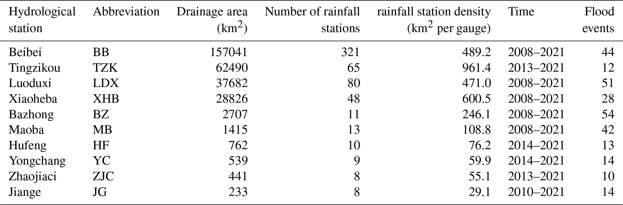
The Jialing River, a major left-bank tributary of the upper Yangtze River, drains an area of 157 041 km², spanning 102°30^′–109° E and 29°40^′–34°30^′ N (Fig. 1). The watershed lies in a subtropical monsoon climate zone where frequent heavy summer rainfall increases both the likelihood and intensity of floods. The region is characterized by hilly and mountainous terrain, numerous tributaries, and steep river gradients, all of which accelerate runoff and heighten susceptibility to localized flooding. Figure 1 shows the spatial distribution of 321 rainfall stations. To ensure representative flood data, ten streamflow stations were selected across a wide range of drainage areas (233–157 041 km²). The Beibei (BB) station at the watershed outlet records an average annual discharge of 2120 m³ s⁻¹ and peak flows up to 44 800 m³ s⁻¹. Tingzikou (TZK) is the only control reservoir on the main stem, while Luoduxi (LDX) and Xiaoheba (XHB) are located downstream of major tributaries. The Bazhong (BZ), Maoba (MB), Hufeng (HF), Yongchang (YC), Zhaojiaci (ZJC), and Jiange (JG) stations lie in small to medium watersheds (233–2707 km²) and are particularly prone to flooding triggered by localized intense rainfall.

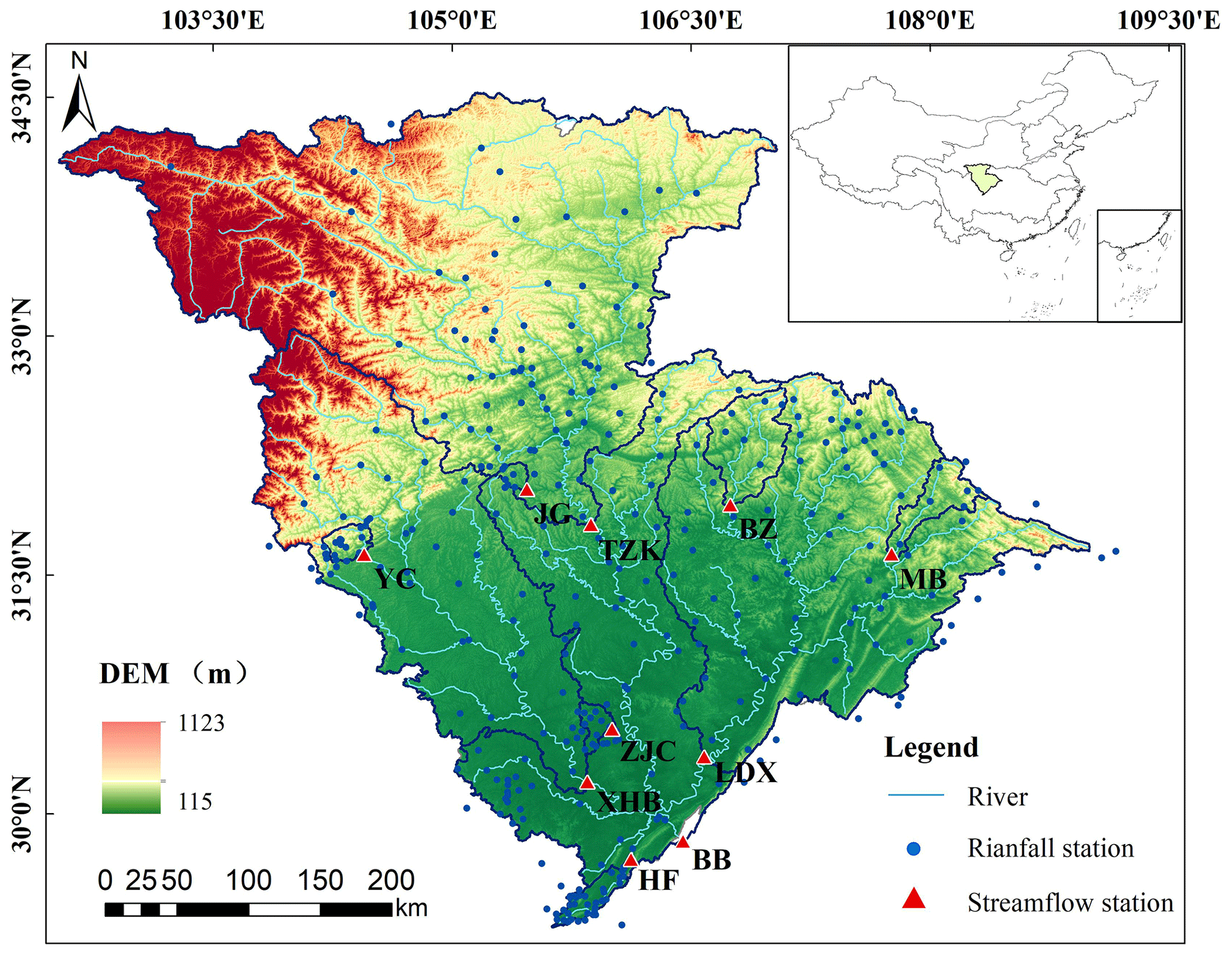
Figure 1 Location of the study area and the distribution of rainfall and streamflow stations.

Hydrological modeling requires multiple types of input data, including rainfall, evaporation, and underlying surface characteristics. Hourly rainfall and streamflow data from the flood season (May to October) during 2008–2021 were used, as summarized in Table 1. Because some stations have shorter observation periods, their records begin after 2008. Rainfall station density across the hydrological stations ranges from 29.1 to 961.4 km² per gauge. The TZK station, located in sparsely populated mountainous terrain, has the lowest density, whereas downstream regions with dense populations and frequent localized floods exhibit much higher densities. Overall, the rainfall network provides adequate spatial coverage across the watershed.

A total of 282 flood events were identified based on the temporal correlation of storm–flood processes among the stations. A 30 m Digital Elevation Model (DEM) was obtained from the United States Geological Survey (https://earthexplorer.usgs.gov/, last access: 1 February 2025). The 1 km soil dataset was sourced from the Food and Agriculture Organization (Batjes, 1997). Evaporation data were taken from the 1 km monthly potential evapotranspiration dataset for China, which was derived using the Hargreaves formula and 1 km temperature data (Peng et al., 2019). Information on the locations and storage capacities of small and medium-sized reservoirs was obtained from the China Reservoir Dataset (Song et al., 2022). The watershed contains 3806 small and medium-sized reservoirs, with a total storage capacity of 3.89 billion m³, equivalent to a runoff depth of 24.7 mm over the entire basin,mainly distributed in the middle and lower reaches.

Table 1 Rainfall and flood data statistics at hydrological stations in the study watersheds.

2.2 Grid-based hydrological model

Choosing an appropriate hydrological model depends on the runoff-generation and routing characteristics of the study area. The study watershed spans multiple climate zones, and the highly uneven spatiotemporal distribution of rainfall leads to diverse and complex runoff-generation mechanisms. The routing process also exhibits strong nonlinear behavior due to the predominance of mountainous terrain and substantial topographic variability. In addition, numerous hydraulic projects within the basin further influence flood dynamics. Considering these characteristics, this study employs the gridded Dahuofang (GDHF) hydrological model, which incorporates the spatial distribution of rainfall, soil properties, and reservoir regulation, making it well-suited for simulating hourly flood events in the study area.

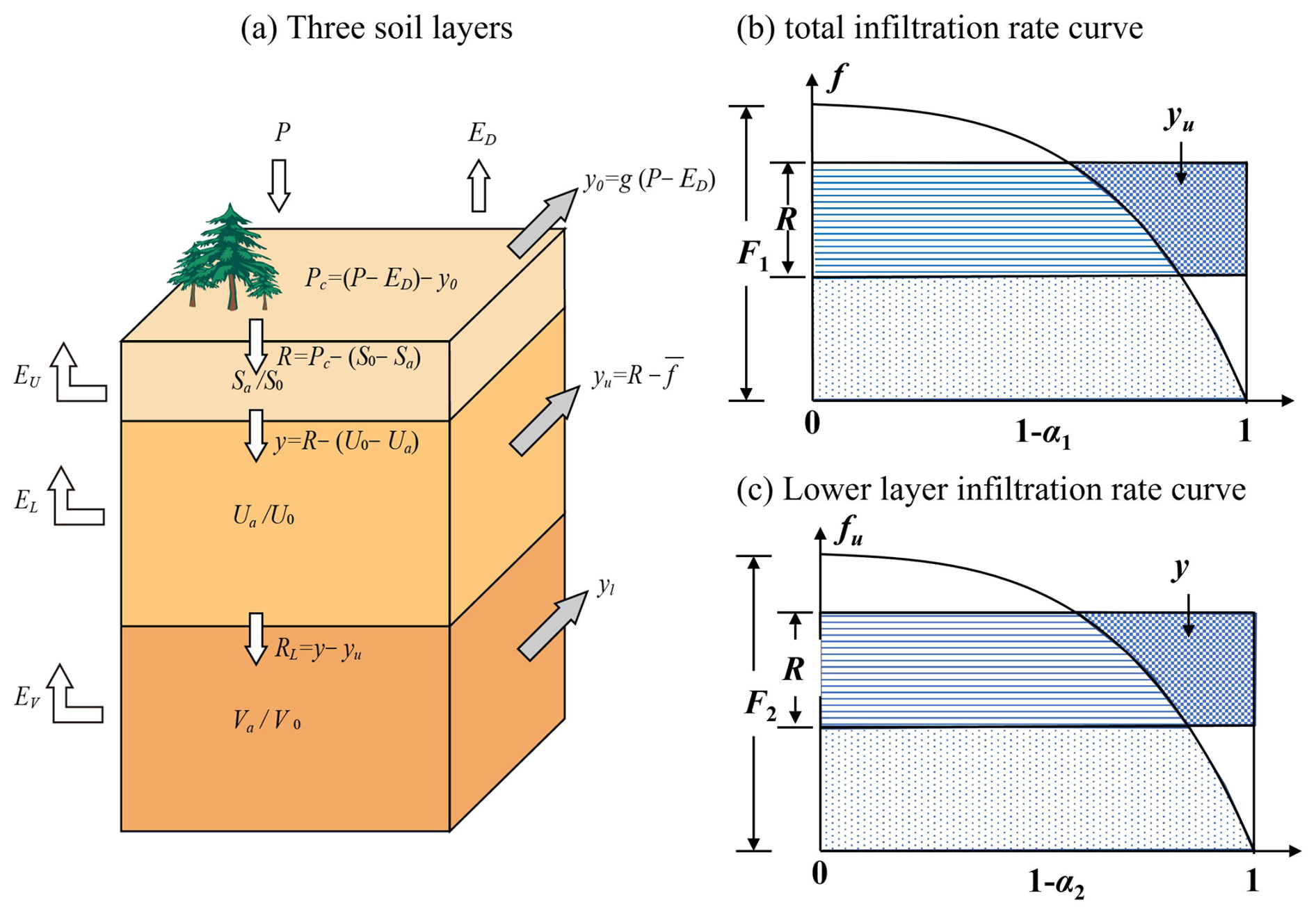
Figure 2 illustrates the soil delineation and runoff generation process of the GDHF model. Soil is divided into three layers – surface, lower, and deep – while a two-layer infiltration curve represents the spatial heterogeneity of the total infiltration rate f and the lower-layer infiltration rate f_u, as shown in Fig. 2b and c. These infiltration characteristics are expressed as:

$$\begin{array}{}\text{(1)}& {\displaystyle }{\mathit{\alpha }}_{\mathrm{1}}=\mathrm{1}-{\left(\mathrm{1}-f/F_{\mathrm{1}}\right)}^{B-\mathrm{1}}\text{(2)}& {\displaystyle }{\mathit{\alpha }}_{\mathrm{2}}=\mathrm{1}-{\left(\mathrm{1}-f_u/F_{\mathrm{2}}\right)}^{B-\mathrm{1}}\end{array}$$

where α₁ and α₂ are the fractions of the area with infiltration rates below f and f_u, respectively; F₁ and F₂ are the maximum total and lower-layer infiltration rates; and B is the shape parameter.

Hillslope routing is simulated using a two-parameter Gamma-distributed unit hydrograph. To better represent the nonlinear behavior of channel flow, a time-varying distributed unit hydrograph that incorporates rainfall intensity is used. Detailed descriptions of the GDHF runoff-generation and routing algorithms can be found in Sect. 2.2 of Li et al. (2024).

Figure 2 Structural diagram of the GDHF hydrological model (Li et al., 2024).

2.3 Experimental design for comparing hourly flood simulations under different spatial resolutions

To evaluate the impact of spatial resolution on hourly flood simulations, the experimental design is shown in Fig. 3. Based on the spatial resolutions of the rainfall, runoff, and underlying surface datasets described in Sect. 2.3.1, four modeling resolutions – 1, 3, 5, and 10 km – were selected for distributed hydrological simulations. GDHF models were constructed at each resolution, followed by parameter calibration and validation at all ten hydrological stations. To assess the benefits of spatial refinement, an additional sub-watershed modeling scheme with fewer computational units was developed, consistent with the configuration used in the operational flood forecasting system of the Jialing River Basin (Zhang et al., 2022). An improvement index (IMP) was defined to quantify the performance enhancement of grid-based models relative to the sub-watershed scheme. The XGBoost model was then applied to evaluate the contribution of flood characteristics to the IMP metrics, identify key resolution-sensitive controlling factors, and reveal the nonlinear effects of these factors on simulation accuracy. Finally, flood events were classified based on these key factors, and the optional spatial resolutions under varying flood characteristics were statistically identified to support the selection of spatial resolution for large-scale hydrological modeling.

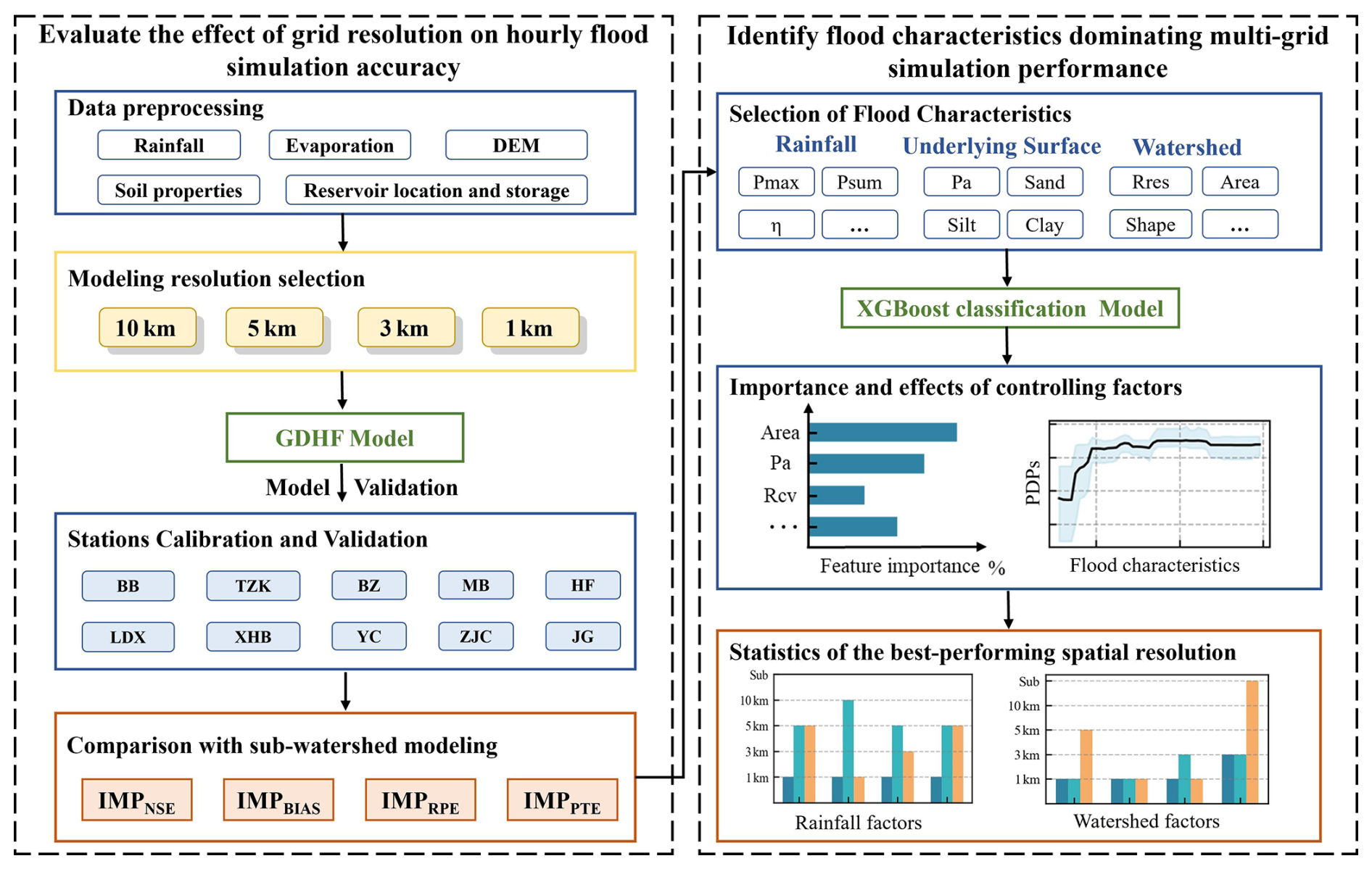
Figure 3 Experimental design on the impact of different spatial resolutions on the accuracy of hourly flood simulations.

2.3.1 Evaluation of GDHF Model Performance at Different Spatial Resolutions

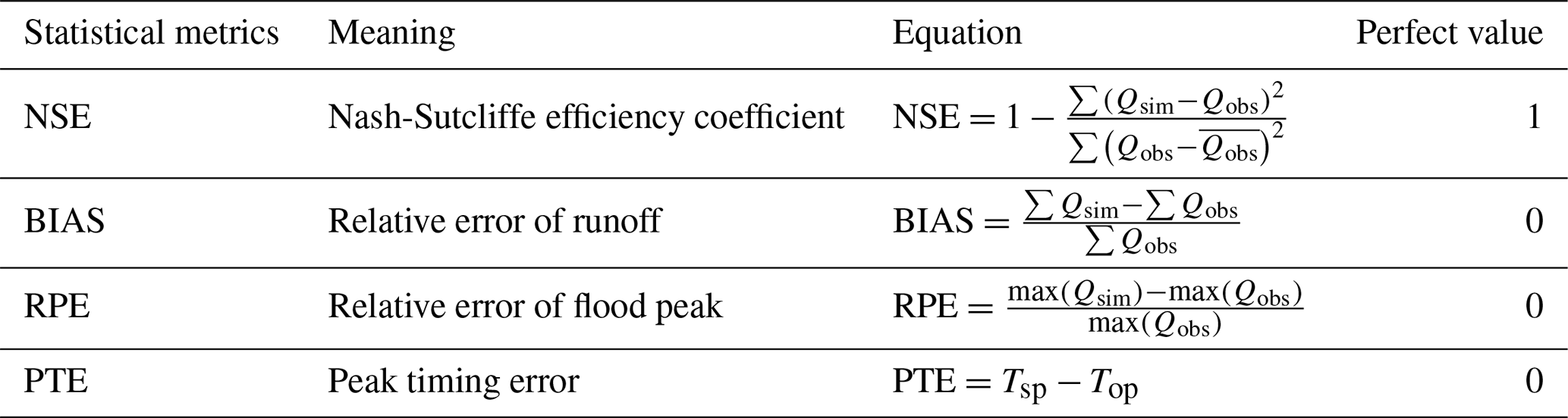
The GDHF models at different spatial resolutions were calibrated using the NSGA-II algorithm. For each spatial resolution, an independent parameter set was calibrated separately for each hydrological station, using 60 % of the flood events for calibration and the remaining 40 % for validation. Model performance was evaluated using several statistical metrics, as summarized in Table 2. The relative error of runoff (BIAS) was employed to assess the accuracy of the runoff generation process, while the relative error of flood peak (RPE) and peak timing error (PTE) were used to evaluate routing performance. The Nash–Sutcliffe efficiency coefficient (NSE) was utilized to assess the overall model performance. In Table 2, Q_sim and Q_obs refer to the simulated and observed discharge, respectively, while T_sp and T_op denote the simulated and observed peak flow times.

Table 2 Statistical metrics used for calibration and evaluation of the GDHF model.

To quantify the extent to which spatial-resolution refinement improves model performance, this study introduces the IMP, which measures the maximum gain achieved by grid-based models relative to sub-watershed modeling. IMP adopts a maximum-based statistic to characterize the upper bound of potential performance gains from spatial-resolution refinement, thereby preventing mean-based statistics from obscuring significant improvements at particular spatial resolutions (Tudaji et al., 2025). IMP_NSE represents the largest improvement in NSE by taking the difference between the highest NSE from all grid-based simulations and that of the sub-watershed model. IMP_BIAS, IMP_RPE, and IMP_PTE represent the greatest reductions in BIAS, RPE, and PTE, respectively, by comparing the minimum absolute BIAS, RPE, and PTE values from the grid-based simulations with those of the sub-watershed model:

$$\begin{array}{}\text{(3)}& {\displaystyle }{\mathrm{IMP}}_{\mathrm{NSE}}=\mathrm{Max}\left\{{\mathrm{NSE}}_{\mathrm{Grid},i}\right\}-{\mathrm{NSE}}_{\text{sub-watershed}}\text{(4)}& {\displaystyle }{\mathrm{IMP}}_{\mathrm{BIAS}}=\left|{\mathrm{BIAS}}_{\text{sub-watershed}}\right|-\mathrm{Min}\left\{\left|{\mathrm{BIAS}}_{\mathrm{Grid},i}\right|\right\}\text{(5)}& {\displaystyle }{\mathrm{IMP}}_{\mathrm{RPE}}=\left|{\mathrm{RPE}}_{\text{sub-watershed}}\right|-\mathrm{Min}\left\{\left|{\mathrm{RPE}}_{\mathrm{Grid},i}\right|\right\}\text{(6)}& {\displaystyle }{\mathrm{IMP}}_{\mathrm{PTE}}=\left|{\mathrm{PTE}}_{\text{sub-watershed}}\right|-\mathrm{Min}\left\{\left|{\mathrm{PTE}}_{\mathrm{Grid},i}\right|\right\}\end{array}$$

Where Grid and sub-watershed refer to the grid-based and sub-watershed models.

2.3.2 Selection of Flood Characteristic Indicators

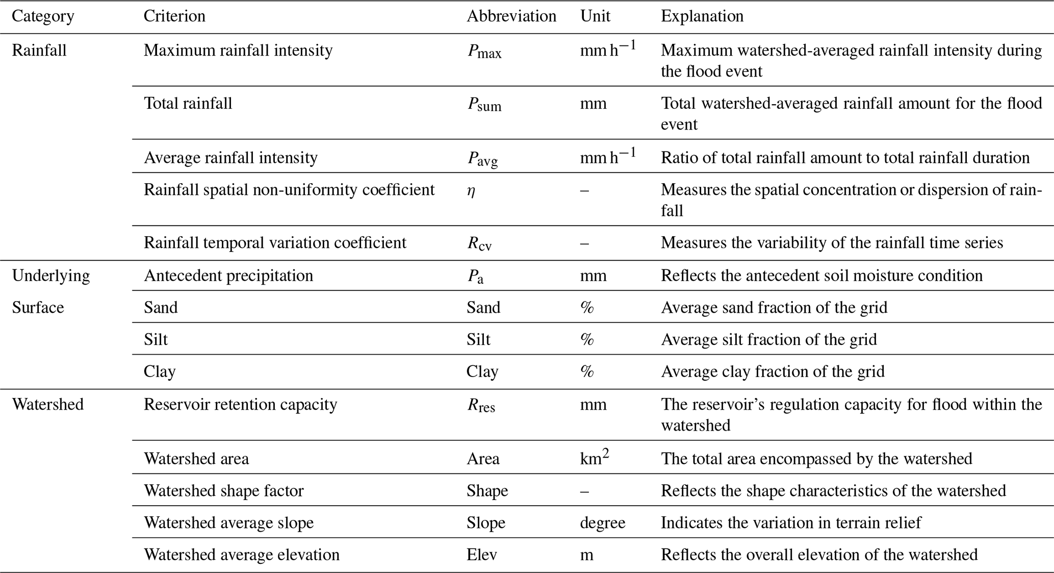
To identify flood characteristics most sensitive to model spatial resolution, fourteen indicators closely related to hydrological processes were selected from three categories: rainfall characteristics, underlying surface conditions, and watershed features. These indicators, derived from existing studies (Wang et al., 2021; Liu et al., 2022; Zhang et al., 2025), effectively represent rainfall, underlying surface conditions, and watershed characteristics. Descriptions of these indicators are provided in Table 3, with detailed calculation methods given in Appendix A.

Rainfall indicators include maximum rainfall intensity (P_max), total rainfall (P_sum), average rainfall intensity (P_avg), rainfall spatial non-uniformity coefficient (η), and temporal variation coefficient (R_cv). These capture the magnitude, intensity, and spatiotemporal variability of rainfall during each flood event. Underlying surface indicators include antecedent precipitation (P_a), reservoir retention capacity (R_res), and soil texture composition (Sand, Silt, and Clay). P_a reflects antecedent soil moisture before each flood event, R_res characterizes flood-regulation capacity, and soil texture variables represent infiltration and storage properties. Watershed characteristic indicators include watershed area (Area), watershed shape (Shape), average slope (Slope), and mean elevation (Elev), which describe the spatial scale, geomorphology, and topographic relief. Collectively, these indicators represent the dominant physical factors affecting runoff generation and routing.

Table 3 Descriptions of the fourteen flood-characteristic indicators.

2.3.3 XGBoost classification model

To examine how flood characteristics influence simulation results across different spatial resolutions, an XGBoost-based classification model was developed to identify key controlling factors most sensitive to spatial resolution. XGBoost, a gradient-boosting decision tree algorithm, is widely used for hydrological applications due to its efficiency and ability to capture nonlinear interactions (Niazkar et al., 2024; Fu et al., 2025). For binary classification, the model predicts the class probability by summing the outputs of multiple regression trees:

$$\begin{array}{}\text{(7)}& {\widehat{y}}_i={\sum }_{k=\mathrm{1}}^K{f}_k\left(x_i\right)f_k\in F\end{array}$$

where ${\widehat{y}}_i$ is the raw score for sample i, f_k is the kth regression tree, and F is the space of all trees.

The XGBoost training procedure consisted of the following steps:

• a.

  Data preprocessing. Four IMP metrics and fourteen flood characteristics were used as model input variables. IMP values are affected by multiple spatial resolutions and are difficult to predict reliably. Therefore, the IMP metrics were converted into binary labels: label = 1 if spatial refinement yields a significant improvement, otherwise, label = 0 (Ekmekcioğlu and Koc, 2022). Because minor improvements in IMP metrics may arise from noise or random fluctuations, labeling all positive changes as 1 could lead to unstable model training and poor generalization (Siam et al., 2022). This study adopts specific thresholds (IMP_NSE > 0.10, IMP_BIAS > 5 %, IMP_RPE > 5 %, or IMP_PTE > 1 h) to identify flood events where spatial grid refinement yields significant improvements in model accuracy and performance. These thresholds are based on the common ranges and practical significance of the metrics in hydrological modelling.

• b.

  Model training. A site-specific leave-one-station-out validation strategy was employed to assess the model's spatial generalization ability. In each iteration, one hydrological station is used as an independent test set, while the remaining stations are used for model training and parameter optimization. This process is repeated for all stations, yielding 10 independent training–testing experiments. Within each training set, five-fold cross-validation is used for XGBoost hyperparameter tuning. This design ensures spatial independence between the training and test data, thereby effectively preventing spatial information leakage.

• c.

  Feature-effect interpretation. Since our study focuses on revealing the global average effects of flood characteristics, partial dependence plots (PDPs) are adopted as a global interpretation method. Compared with the SHAP method, PDPs provide a clearer and more intuitive visualization of the marginal effect of each flood characteristic on model predictions. Moreover, PDPs have been widely used in previous studies to investigate the nonlinear impacts of key flood features (Wang et al., 2026; Yao et al., 2026). Therefore, PDPs were chosen to visualize how each flood characteristic affects the IMP. For each plot, one feature was varied while all others were averaged over their empirical distributions. PDPs were averaged across 100 runs, and 95 % confidence intervals were provided to indicate uncertainty.

2.3.4 Determination of the optimal spatial resolution for hydrological modeling

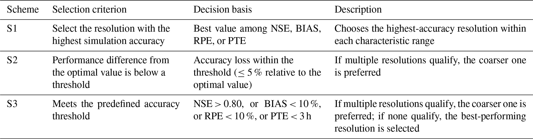
To systematically identify appropriate spatial resolutions under varying flood characteristics, this study employs three resolution-selection schemes based on the model performance. The purpose of setting three different schemes is to select the optimal spatial resolution from both accuracy and computational efficiency perspectives, as the optimal resolution is not unique. In the S1 scheme, the optimal spatial resolution is determined solely based on flood simulation accuracy. In contrast, the S2 and S3 schemes, while satisfying predefined accuracy thresholds (e.g., NSE > 0.8 for S2 and relative error ≤ 5 % for S3), prioritize selecting coarser grids to improve computational efficiency. Observing the differences in the optimal spatial resolutions obtained from these schemes provides valuable insight for selecting appropriate spatial resolutions in large-watershed modeling. Table 4 summarizes these three spatial-resolution selection schemes.

Table 4 Summary of the spatial resolution selection schemes employed in this study.

3 Hydrological modeling and evaluation at different spatial resolutions

The GDHF model at different spatial resolutions requires watershed unit delineation, spatial interpolation of rainfall, and discretization of underlying surface characteristics. The watershed unit delineation results are shown in Fig. B1, where the numbers of units for the sub-watershed scheme and for the 10, 5, 3, and 1 km spatial resolutions are 107, 1662, 6353, 17 283, and 152 243, respectively. Hourly rainfall observations were interpolated into cells of different resolutions using the Inverse Distance Weighting (IDW) method and used as rainfall inputs for the GDHF model.

The modeling process emphasizes spatial discretization of the underlying surface, including soil type, reservoir distribution, and river routing topology. Runoff-related parameters – such as field capacity, wilting point, and reservoir storage capacity – were derived from soil type, soil thickness, and the spatial distribution and storage capacities of small- and medium-sized reservoirs. Routing parameters (e.g., channel length, flow direction, and slope) were calculated from DEM data. Figure 4 shows the spatial parameterization of the GDHF model using the 10 km resolution as an example.

As illustrated in Fig. 4a, Loam and Silty Loam are the dominant soil types in the watershed. Figure 4b presents the soil moisture capacity (S₀+U₀) of the surface and lower layers, estimated from soil type and soil thickness, with values ranging from 130 to 170 mm and showing pronounced spatial variability. Figure 4c shows the flow directions and river network topology extracted from the DEM, indicating that 1662 grid cells ultimately drain to the watershed outlet. Figure 4d illustrates the influence of reservoir regulation, which is weak in upstream areas but becomes significant in downstream regions.

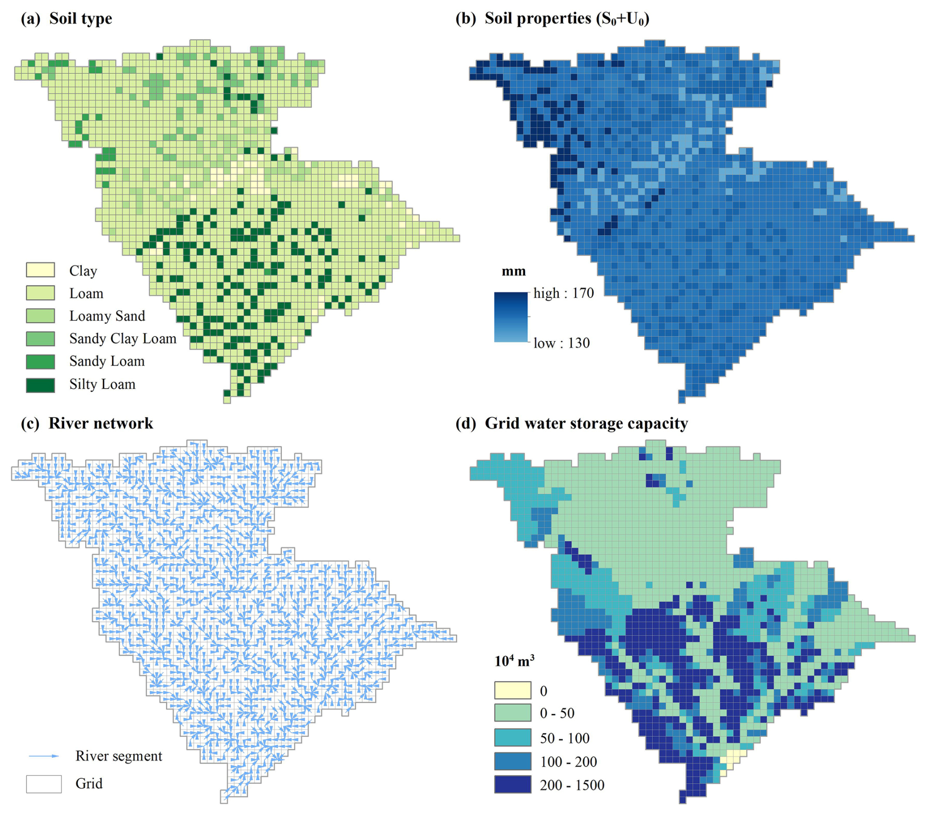
Figure 4 Spatial distribution of (a) the soil types, (b) soil properties, (c) river network, and (d) grid water storage capacity.

4 Results and Discussion

4.1 Comparison of flood simulation accuracy at different spatial resolutions

Based on the evaluation metrics described in Sect. 3, the performance of flood simulations under different spatial modeling resolutions was compared for both the calibration and validation periods across the ten stations (Fig. 5). The evaluation metrics | BIAS |, | RPE |, and | PTE | represent the average absolute errors of all flood events at each station.

Figure 5 shows that flood simulation accuracy varies substantially across spatial resolutions. Among all configurations, the 1 km grid performs the best: NSE values exceed 0.80 at all stations, while | BIAS | and | RPE | remain around 10 % and 15 %, respectively, and | PTE | consistently stays below 5 h. This indicates that the 1 km resolution effectively captures the runoff-generation and flow-routing processes of flood events. In contrast, the sub-watershed model, which contains the fewest computational units, exhibits the lowest performance, with NSE values dropping to approximately 0.60 at several stations and flood-volume and peak-flow errors exceeding 20 %.

The sensitivity of simulation performance to spatial resolution differs markedly across station types. For stations with large drainage areas (such as BB), differences in simulation accuracy among the 1, 3, 5, and even 10 km grids are minimal, and the sub-watershed model can still reproduce the major flood characteristics reasonably well. Aerts et al. (2022) also observed this phenomenon using the daily CAMELS dataset: finer spatial resolution does not bring significant improvement at the watershed outlet. In contrast, for stations with smaller drainage areas (BZ, MB, HF, YC, ZJC, and JG), refining the spatial resolution substantially enhances the representation of runoff generation and flow routing, thereby significantly improving simulation accuracy (Modi et al., 2025).

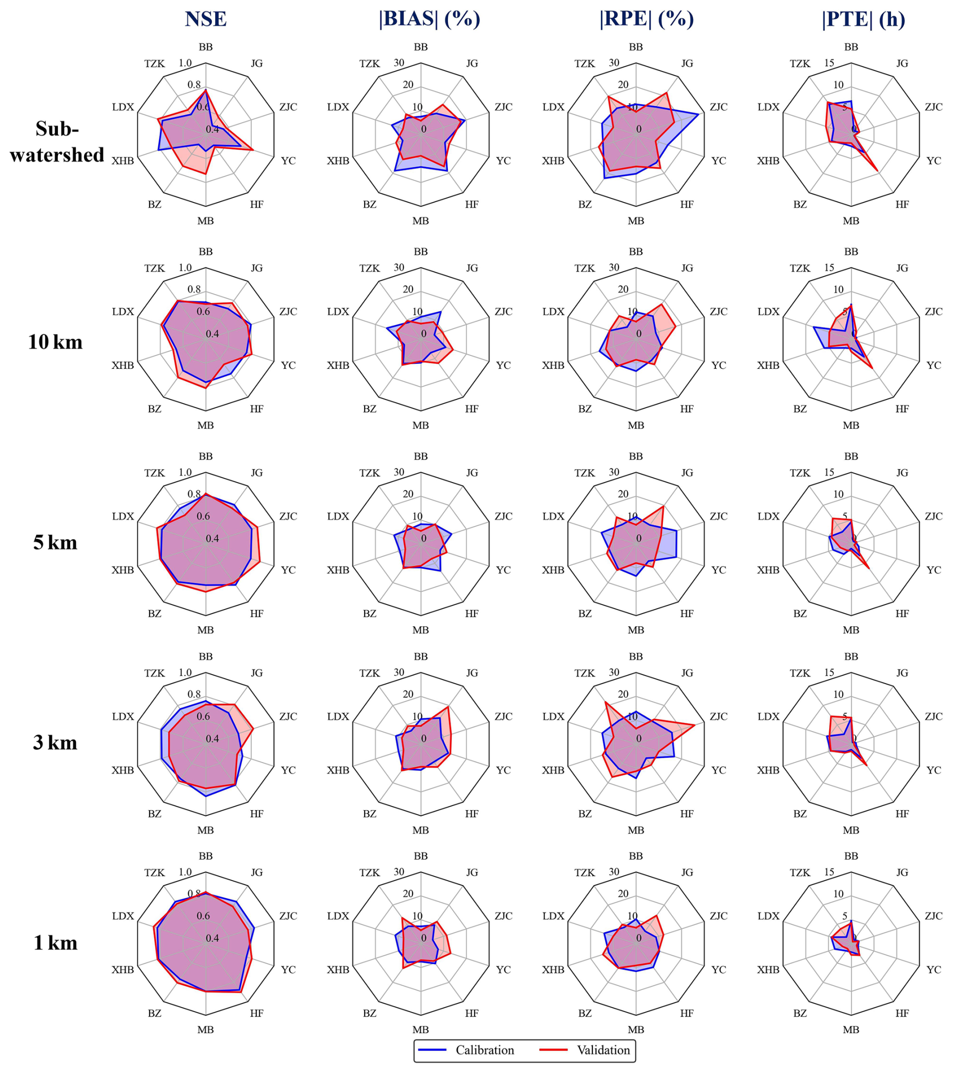
Figure 5 Evaluation metrics for simulating hourly flood events across different spatial resolutions during calibration and validation periods.

To further assess spatial resolution effects for stations of different areas, the stations were classified into two categories: main-stream control stations and small-to-medium watersheds. The control stations (BB, TZK, LDX, and XHB) are located at watershed outlets or major tributaries, with drainage areas of 28 826–157 041 km². The remaining stations represent small-to-medium watersheds with drainage areas of 233–2707 km².

Figure 6a shows that for small and medium-sized watersheds, NSE values increase substantially as the spatial resolution is refined. Compared with coarse-resolution modeling (sub-watershed, 10, and 5 km), the 3 and 1 km grids capture the rising and recession limbs of the hydrograph much more accurately. In contrast, for control stations, refining the spatial resolution results in only marginal improvements in NSE. Figure 6b, c, and d further indicate that for small-to-medium watersheds, finer spatial resolution leads to substantial improvements in | BIAS |, | RPE |, and | PTE |, whereas for control stations, refining the spatial resolution yields almost no improvement in simulated flood volume, peak flow, or peak timing. This contrast reflects fundamental differences in hydrological nonlinearity across watershed areas. In large watersheds, floods originate from multiple sub-regions, and nonlinear processes become smoothed during flow aggregation, reducing the overall nonlinearity of the flood response. Small watersheds are highly sensitive to localized rainfall, steep gradients, and rapid flow routing, leading to strong nonlinear responses (Wilkinson and Bathurst, 2018). Consistent with these findings, Jiang et al. (2025) also reported that higher-resolution CaMa-Flood models improve daily peak-flow simulation, with the most pronounced improvements occurring in smaller tributaries.

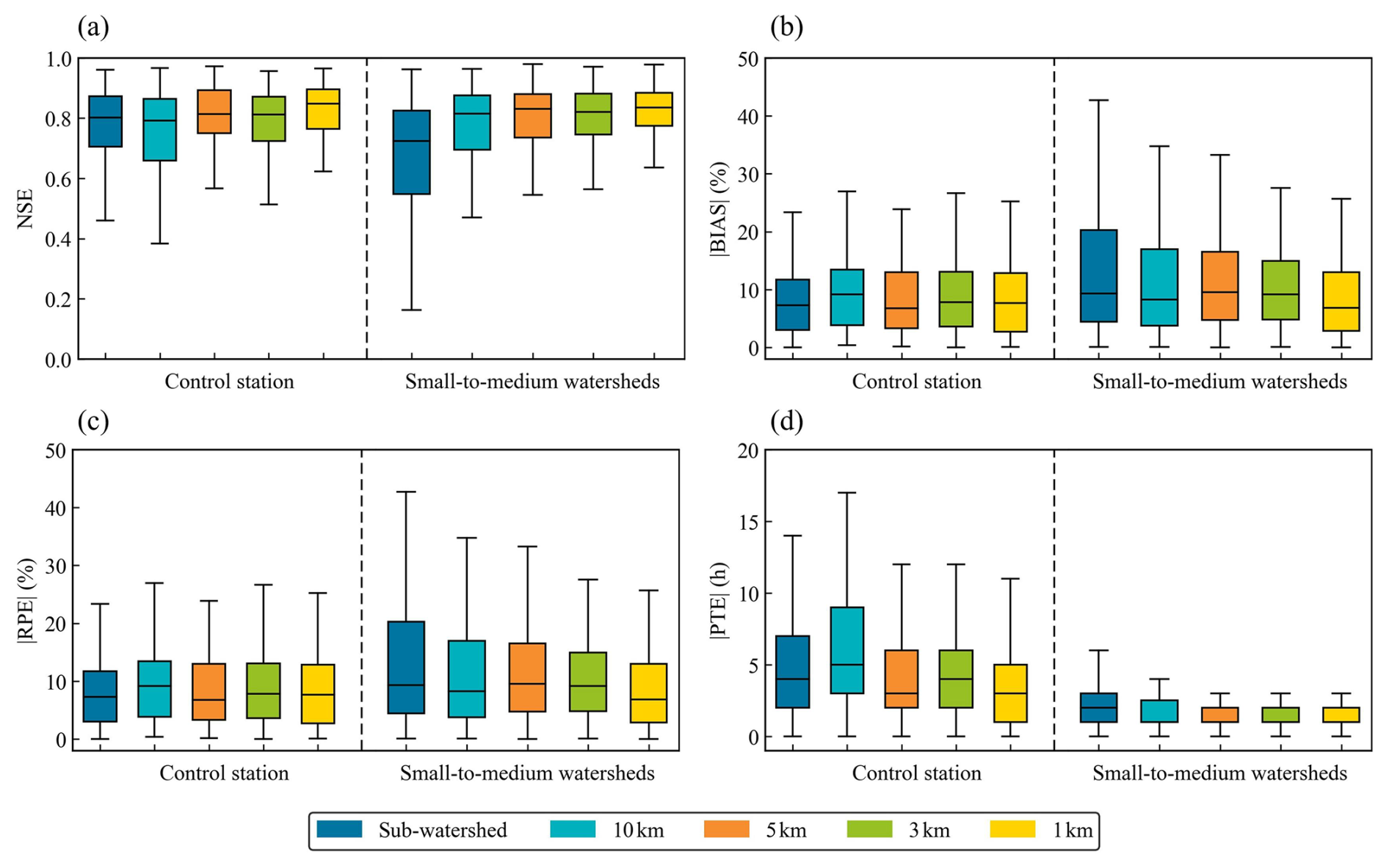
Figure 6 Comparison of flood simulation results across various spatial resolutions for stations with different areas.

4.2 Comparison of computational time at different spatial resolutions

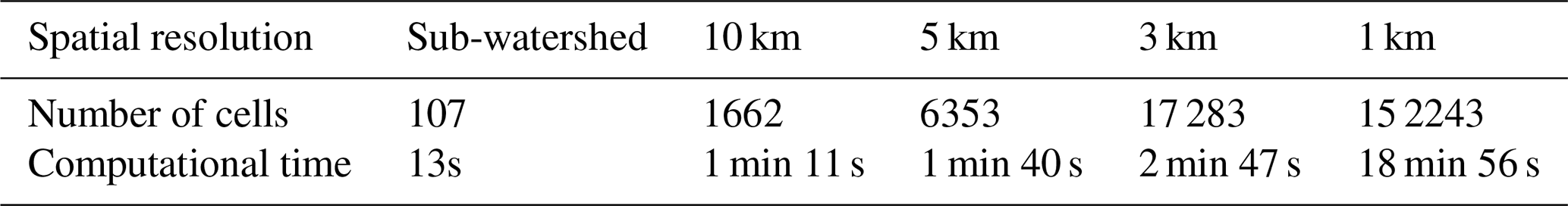
To compare the computational time under different spatial resolutions, the flood event from 22 to 29 August 2020, was selected. After applying a 10 d warm-up period, the effective simulation spanned 17 d, consisting of 408 time steps. All computations were performed on a laptop equipped with an 11th Gen Intel^® Core™ i7-11800H processor (8 cores and 16 threads). The corresponding computational times are summarized in Table 5.

The results show that as spatial resolution is refined, the number of grid cells increases exponentially, leading to a sharp rise in computational time. The sub-watershed and 10 km simulations require only about 13 s and 1 min 11 s, respectively, whereas the 1 km simulation requires approximately 18 min 56 s. Aerts et al. (2022) also found that computational time does not scale linearly with the number of grid cells when running models at different spatial resolutions on high-performance computing equipment. Moreover, real-time flood forecasting requires preparing large volumes of hydrological input data – such as rainfall interpolation and initial soil moisture conditions – which further increases computational burden. Therefore, applying a 1 km spatial resolution to a large watershed significantly increases computational cost, making it difficult to meet the efficiency requirements of real-time flood forecasting.

Table 5 Computational time for simulating a single flood event at different spatial resolutions.

4.3 Identifying controlling factors of spatial resolution with XGBoost

Flood characteristics identified in Sect. 2.3.2 as influential to runoff generation and routing were examined as potential controls for determining the appropriate spatial resolution. To ensure their robustness, we analyzed their relationships with the IMP metrics. Figure 7 presents the Spearman correlation coefficients (ρ) and significance levels for fourteen flood characteristics and four IMP metrics. The sign of ρ indicates positive or negative correlation, values closer to ±1 represent stronger monotonic relationships, and values near 0 indicate weak associations. Asterisks denote the corresponding significance levels.

The results show that P_max and P_avg are strongly positively correlated (ρ=0.90), indicating close consistency between maximum and average rainfall intensity. Thus, either can serve as the representative rainfall variable in the subsequent XGBoost model. The variable η also exhibits significant positive correlations with P_max and P_avg (ρ=0.78 and 0.80). Regarding underlying surface characteristics, Area shows strong negative correlations with P_max, P_avg, and η ($\mathit{\rho }=-\mathrm{0.82}$, −0.83, and −0.79), suggesting that as Area increases, rainfall intensity decreases and rainfall spatial variability increases. Elev is negatively correlated with Silt ($\mathit{\rho }=-\mathrm{0.69}$) and positively correlated with Slope (ρ=0.59). R_res also shows a significant negative correlation with Slope ($\mathit{\rho }=-\mathrm{0.73}$), indicating that reservoir regulation weakens in higher-elevation watersheds.

Although the ρ values between these flood characteristics and four IMP metrics are not particularly high, many characteristics – such as Area and several rainfall- and surface-related indicators – still exhibit statistically significant relationships with IMP. The strong associations between these characteristics and especially IMP_NSE support the validity of the selected potential driving factors and provide a solid foundation for identifying key features in subsequent analyses.

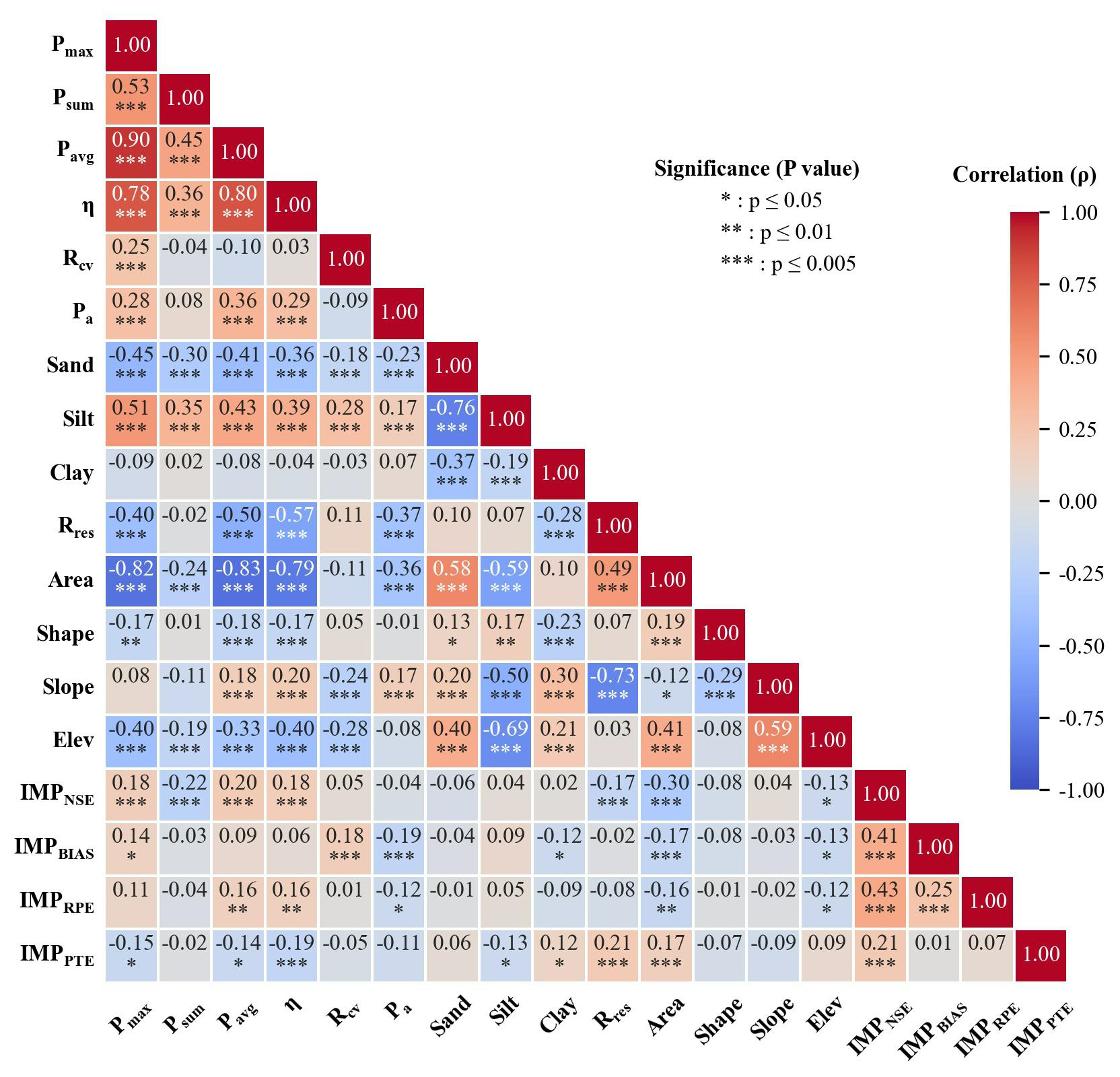
Figure 7 Spearman correlation analysis results between fourteen flood characteristics and four IMP metrics.

To identify how potential driving factors influence flood simulations across different spatial resolutions, this study employs an XGBoost model to identify key resolution-sensitive factors, with model configurations detailed in Sect. 2.3.3. Because the ρ between P_max and P_avg exceeds 0.90, indicating strong multicollinearity, P_avg was excluded, and P_max was retained as the representative rainfall intensity indicator. For all four IMP metrics, the trained XGBoost model achieved average recall values of 78.3 %–97.8 % on the training sets and 64.9 %–73.0 % on the test sets, with corresponding AUC of 0.78–0.98 (training) and 0.65–0.76 (test). These results indicate satisfactory fitting capability and acceptable generalization performance, comparable to the AUC range (0.75–0.83) reported in similar XGBoost-based classification studies (Kumar et al., 2026).

Figure 8 presents the mean contribution rates of the driving factors and their standard deviations across the IMP metrics. For the IMP_NSE metric (Fig. 8a), Area, P_sum, and Slope are the primary contributors, explaining 40.9 % of the model output, with Area showing the highest importance and thus serving as the key controlling factor. Previous studies have also confirmed the importance of drainage area for the selection of spatial resolution by evaluating the improvement in accuracy achieved through spatial resolution refinement across different drainage areas (Aerts et al., 2022; Jiang et al., 2025).

For the IMP_BIAS metric (Fig. 8b), P_a, Clay, and R_cv contribute most significantly (35.4 %), indicating that antecedent soil moisture, soil clay content, and maximum rainfall intensity – three variables strongly linked to runoff generation – jointly govern the IMP_BIAS response. For the IMP_RPE metric (Fig. 8c), P_max, P_sum, and Elev are the dominant features, accounting for 32.6 % of the contribution. For the IMP_PTE metric (Fig. 8d), Slope, R_res, and Clay emerge as the main drivers, with a combined contribution of 26.3 %. These results highlight that rainfall characteristics, together with Elev, Slope, R_res, and Clay, are critical factors affecting peak discharge and time to peak. Moreover, Luo et al. (2025) identified rainfall, elevation, and slope as key drivers of flash floods using the SHAP method, and these factors show strong consistency with the key controlling factors of spatial resolution identified in this study. Overall, the XGBoost analysis reveals that the flood characteristics controlling improvements in multi-grid simulation performance differ substantially across the various IMP evaluation metrics.

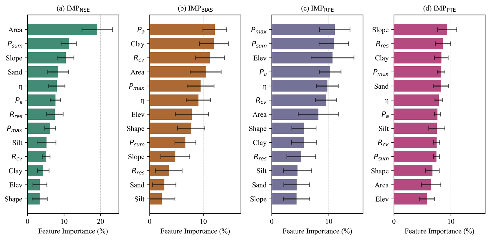
Figure 8 Importance ranking and contribution rates of flood characteristics based on the XGBoost model.

4.4 Nonlinear effects of controlling factors on flood simulation accuracy

To further clarify how key flood characteristics influence the IMP values, this study uses PDPs to illustrate the relationships between each characteristic and the IMP, as shown in Fig. 9.

For IMP_NSE, Fig. 9a shows that smaller watersheds are more likely to benefit from spatial refinement, and the probability of improvement declines progressively as watershed area increases. In addition, Fig. 9b and c indicate that lower P_sum and lower Slope values are associated with higher probabilities of IMP_NSE improvement. For IMP_BIAS, Fig. 9d identifies P_a as a key determinant: smaller P_a values increase the likelihood of improving IMP_BIAS. Figure 9e further shows that lower Clay content also favors performance gains. Moreover, Fig. 9f demonstrates that larger R_cv – reflecting more pronounced temporal variability of rainfall – corresponds to an increased probability of improving IMP_BIAS.

For IMP_RPE, Fig. 9g shows that higher P_max enhances the likelihood of improvement, while Fig. 9h and i indicate that lower P_sum and lower Elev likewise increase the probability of IMP_RPE improvement. For IMP_PTE, Fig. 9j and k reveal that watersheds with gentler slopes and higher R_res (i.e., stronger reservoir regulation effects) are more likely to achieve reductions in peak-timing error through spatial refinement. However, Fig. 9l shows that the influence of Clay on IMP_PTE fluctuates without a clear monotonic trend.

Overall, Area exerts the most pronounced nonlinear effect on the probability of improvement for IMP_NSE. Rainfall characteristics – particularly P_sum, P_max,and R_cv – play critical roles in determining improvement probabilities for IMP_NSE, IMP_BIAS, and IMP_RPE. In addition, several underlying surface characteristics, including P_a, Slope, Clay, Elev, and R_res, also contribute to variations in the effectiveness of IMP improvements.

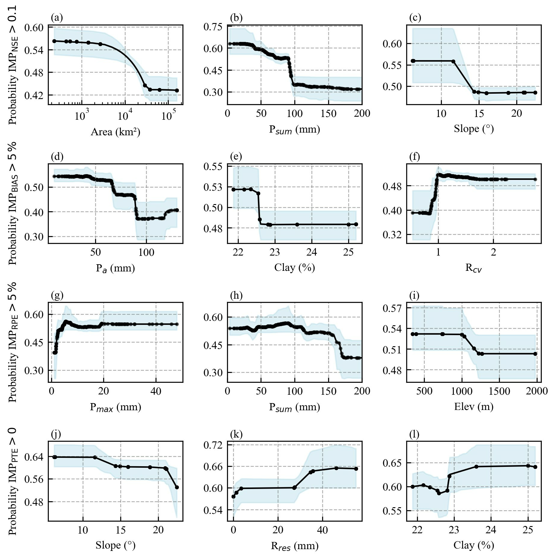
Figure 9 PDPs of the predicted probabilities of improvement in four IMP metrics based on different flood characteristics.

To validate the nonlinear influence of flood characteristics on the IMP revealed by the PDPs, flood events were classified according to their characteristic values, and the IMP metrics were statistically analyzed across categories, as shown in Fig. 10.

Figure 10a shows that when the Area is small (<104 km²), particularly below 10³ km², most flood events yield positive IMP_NSE values, indicating that small and medium-sized watersheds are most responsive to spatial refinement. As the watershed area increases, the median IMP_NSE approaches zero, indicating that spatial refinement offers limited NSE improvement in large watersheds. Thus, Area is the dominant factor governing whether NSE can benefit from finer spatial resolution. Figure 10b further shows that IMP_NSE improves most substantially when P_sum < 100 mm, whereas flood events with larger rainfall amounts (P_sum>100 mm) exhibit much weaker sensitivity. Similarly, Fig. 10c indicates that when Slope < 10°, IMP_NSE values are almost entirely positive, suggesting that watersheds with gentler terrain benefit more from spatial refinement.

For IMP_BIAS, Fig. 10e demonstrates a marked improvement in IMP_BIAS when P_a < 80 mm – especially < 40 mm – highlighting the nonlinear control of antecedent soil moisture on flood-volume simulations. Figure 10d shows that when Clay < 22.5 %, most events have positive IMP_BIAS values, implying that low clay content favors reductions in flow-volume bias. As shown in Fig. 10f, the improvement in IMP_BIAS is particularly significant when the rainfall temporal variability coefficient (R_cv) exceeds 1.5.

Figure 10g suggests that IMP_RPE varies little across P_max categories, whereas Fig. 10h shows that IMP_RPE improves noticeably when P_sum < 100 mm. Figure 10i reveals that low-elevation basins tend to achieve greater RPE improvement, with median IMP_RPE decreasing as Elev increases. For IMP_PTE, Fig. 10j shows that Slope < 10° yields the greatest reduction in peak-timing error. Figure 10k further indicates that larger R_res values – representing stronger reservoir regulation – are associated with greater improvements in IMP_PTE, suggesting that regulated basins benefit more from spatial refinement than natural watersheds. Finally, Fig. 10l shows no clear trend between IMP_PTE and Clay, implying that peak-timing errors are influenced primarily by terrain and reservoir regulation rather than Clay content. Overall, flood characteristics impose distinct and nonlinear controls on the effectiveness of spatial resolution refinement.

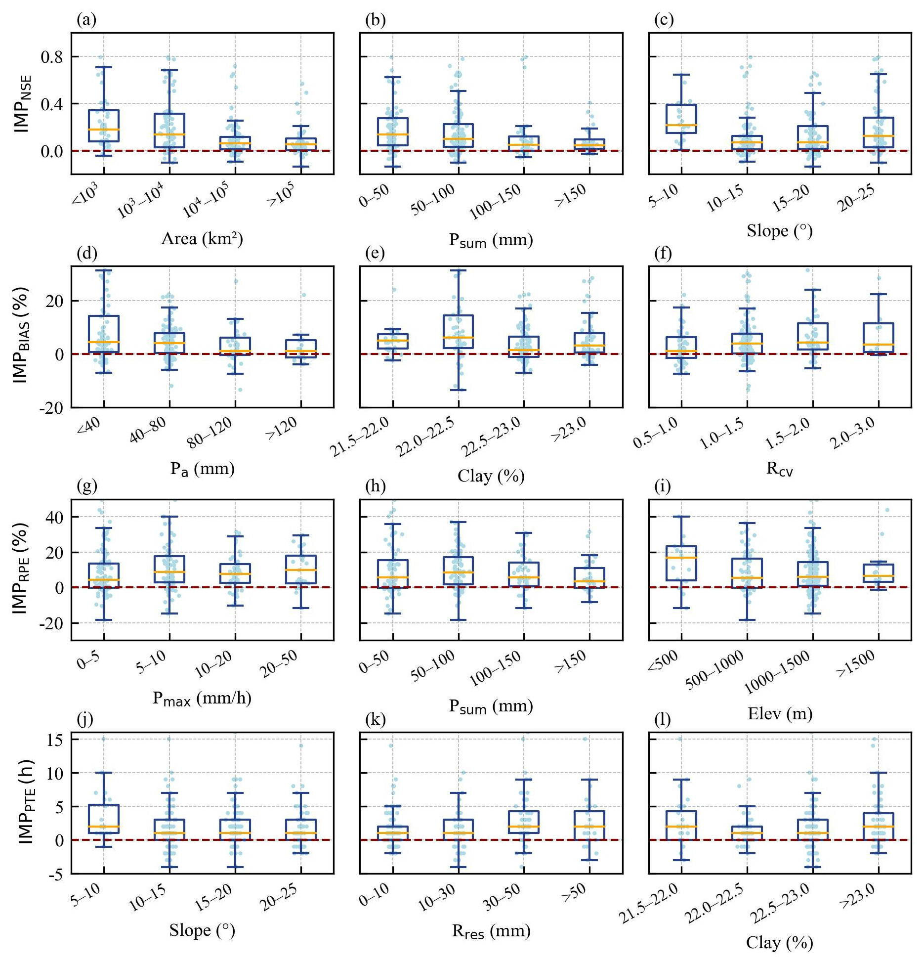
Figure 10 Boxplots of IMPNSE, IMPBIAS, IMPRPE, and IMPPTE metrics under different flood characteristics.

4.5 Statistical analysis of optimal spatial resolution based on controlling factors

The analysis in Sect. 4.4 indicates that, under specific flood-characteristic conditions, refining the spatial resolution can substantially improve flood-simulation accuracy compared with sub-watershed modeling. Building on this, the present section further compares model performance across different spatial resolutions to identify the optimal spatial resolution under various controlling-factor scenarios. Figure 11 illustrates how NSE, BIAS, RPE, and PTE vary with flood characteristics at different spatial resolutions.

Overall, within the characteristic ranges identified in Sect. 4.4, finer spatial resolutions generally yield higher simulation accuracy than sub-watershed modeling, as reflected by increased NSE and decreased BIAS, RPE, and PTE values. The improvements are particularly pronounced for small watersheds (Area < 104 km²), gentle terrain (Slope < 10°), or low cumulative rainfall (P_sum < 100 mm), where the 1, 3, and 5 km grids all outperform the sub-watershed approach. In contrast, for large basins (Area > 104 km²), wetter antecedent soil conditions (P_a > 80 mm), or other conditions characterized by weaker flood nonlinearity, differences among spatial resolutions diminish, and spatial refinement offers limited benefits.

Although the 1 km grid generally achieves the best performance across all four metrics, Fig. 11 also shows that in many characteristic ranges, the performance differences between resolutions are relatively small. This suggests that higher spatial resolutions do not necessarily yield proportional improvements. Therefore, spatial refinement should be applied selectively, guided by the degree of flood-process nonlinearity and the sensitivity of simulations to local rainfall and underlying-surface heterogeneity.

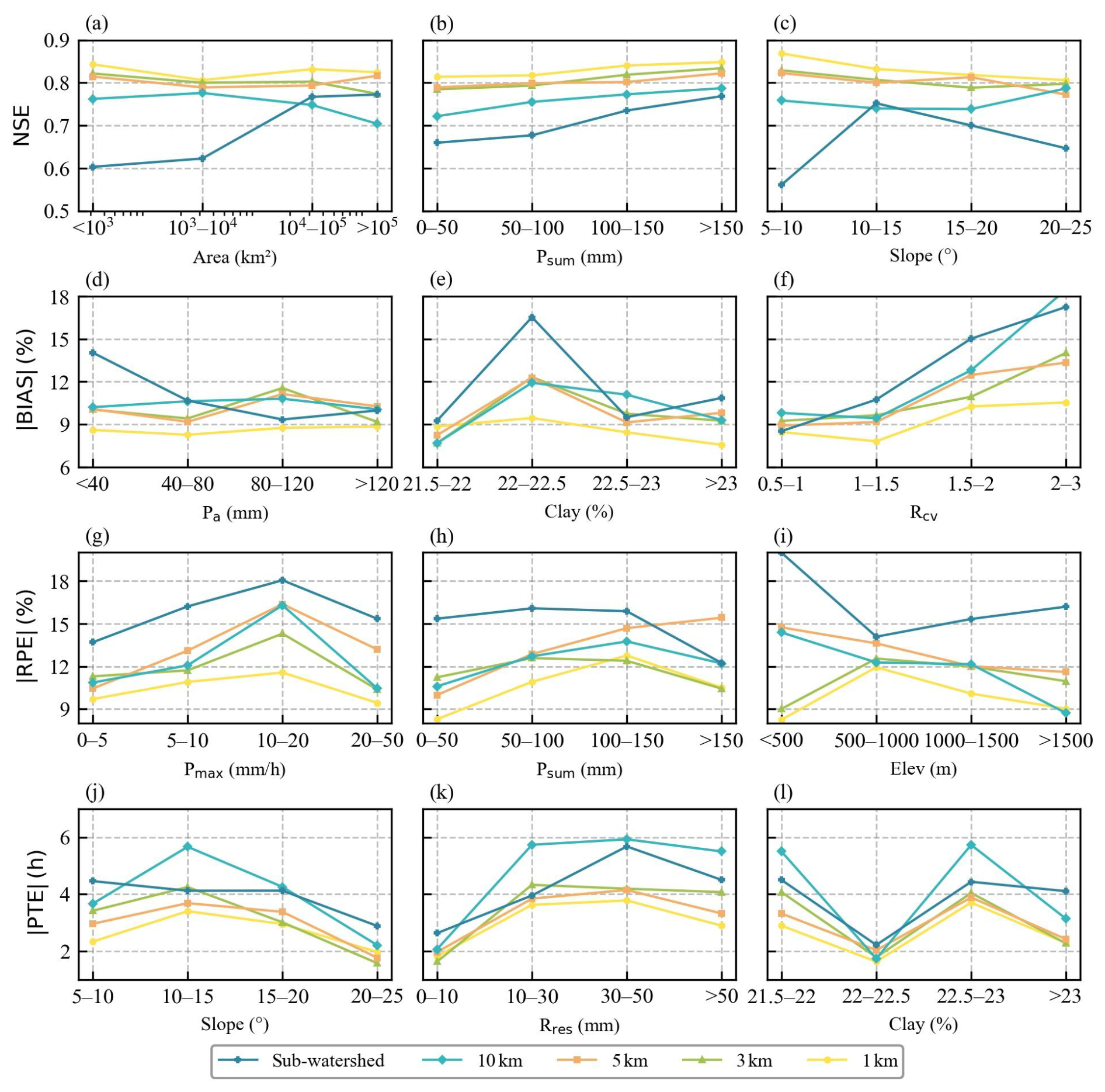
Figure 11 Variations of flood simulation accuracy with flood characteristics under different spatial resolutions.

To systematically identify appropriate spatial resolutions under varying flood characteristics, this study employs three resolution-selection schemes (Sect. 2.3.4) based on the performance patterns observed in Fig. 11. Figure 12 presents the appropriate spatial resolutions for different flood characteristic categories under the three schemes.

The statistics from S1 show that fine grids (1 and 3 km) generally perform best across most characteristic intervals. Nonetheless, notable exceptions exist: when the soil clay content falls within 21.5 %–22 %, or when basin elevation exceeds 1500 m, the 10 km grid becomes the preferred resolution. This indicates that under these specific conditions, coarser grids may in fact yield higher accuracy for certain performance metrics.

For the NSE metric, S2 tends to select 3–5 km grids across multiple characteristic ranges. This is because, under the criterion that a resolution is acceptable when its relative accuracy loss does not exceed 5 %, medium-resolution grids can already achieve NSE performance very close to that of the optimal resolution. In contrast, for the BIAS, RPE, and PTE metrics, the spatial resolutions recommended by S2 are largely identical to those selected by S1. This indicates that, under these characteristic conditions, the performance gaps between the non-optimal resolutions and the optimal one remain relatively large, making it difficult for them to satisfy the 5 % accuracy-loss threshold.

For S3, the NSE metric tends to favor the 5 km spatial resolution because this resolution already meets the predefined accuracy criterion (NSE > 0.80), making further refinement unnecessary. For BIAS, when antecedent soil moisture is high (P_a > 80 mm), clay content is relatively large, or rainfall exhibits a more uniform spatial distribution (R_cv < 1.5), S3 tends to recommend coarser resolutions (such as 10 km or Sub-watershed). These resolutions are sufficient to satisfy the accuracy threshold (BIAS < 10 %), and therefore, higher spatial resolutions are not required. In contrast, for the RPE and PTE metrics, coarse grids often fail to meet the predefined accuracy requirements (RPE < 10 %, PTE < 3 h). As a result, the S3 selections align closely with those of S1, more frequently recommending finer resolutions (1–3 km).

In summary, selecting spatial resolutions based on flood characteristics not only ensures reliable flood-forecasting accuracy but also avoids unnecessary computational costs associated with blindly refining model resolution, thereby providing a scientific basis for determining appropriate spatial resolutions in large-watershed flood forecasting.

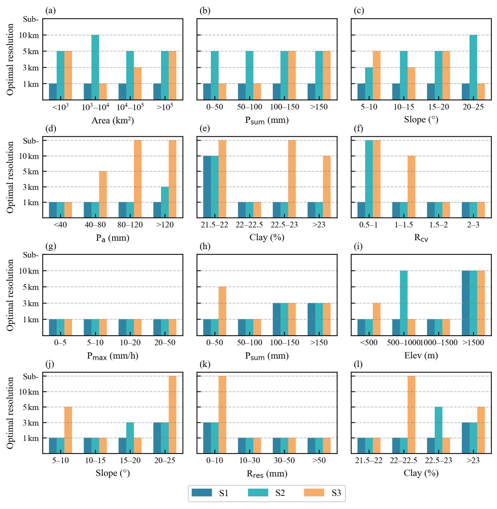
Figure 12 Spatial resolution recommendations for different flood characteristic categories based on the three schemes.

4.6 Effect of rainfall station density on flood simulation accuracy

To evaluate the effectiveness of refining model spatial resolution under sparse rainfall observations, this section reduces the number of rain gauges by 25 %, 50 %, and 75 % and examines the influence of station density on flood-simulation accuracy across multiple spatial resolutions. To avoid representation issues associated with random gauge removal, the Thiessen polygon method was used to compute the weight of each station. Rain gauges were then ranked in descending order of weight, and those with lower weights were removed first to ensure that the remaining stations best represented the spatial distribution of rainfall across the study area.

Given that the control stations are less sensitive to changes in spatial modeling resolution than small and medium-sized watersheds (Fig. 6), this section focuses on all small and medium-sized watersheds for analysis. Figure 13 shows the flood simulation accuracy across different spatial resolutions under varying rainfall station removal ratios (0 %, 25 %, 50 %, and 75 %). The results show that when rainfall station density is high (e.g., no removal or only 25 % removal of gauges), flood simulation accuracy increases significantly with finer spatial resolution, and the median NSE is higher for fine grids (1–3 km). However, when rainfall station density is substantially reduced (with 50 % or 75 % of the gauges removed), the differences in simulation accuracy among different spatial resolutions become much smaller, and spatial refinement provides only limited improvement to flood-simulation accuracy. This indicates that under sparse gauge conditions, even fine-resolution grids cannot substantially improve simulation results. Huang et al. (2019) also found that, in watersheds with sparse gauge networks, refining spatial resolution yields model performance similar to that of the lumped model. Furthermore, Ziaee and Abedini (2023) also emphasized that rain gauge density is a key factor affecting peak flow, and insufficient monitoring station density often leads to underestimation of the peak flow. Therefore, when selecting the spatial resolution for modeling, the spatial representativeness of the rainfall data must be carefully considered.

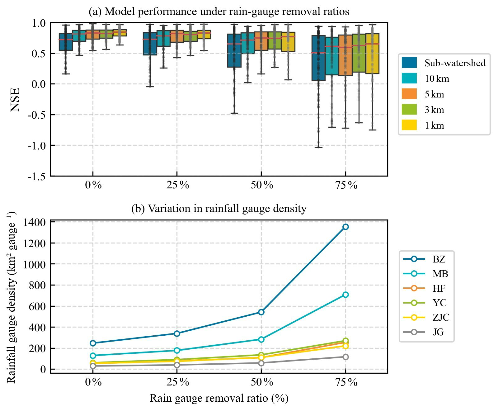
Figure 13 Flood simulation accuracy across different spatial resolutions under varying rainfall station removal ratios (0 %, 25 %, 50 %, and 75 %).

Building on this analysis, three representative flood events with notable accuracy gains from spatial-resolution refinement were selected to further assess whether fine-resolution grids (1 km) remain effective under reduced rainfall station density. The resulting changes in rainfall spatial distribution and flood-simulation performance across different gauge densities are shown in Fig. 14.

Figure 14a shows that as the gauge removal ratio increases from 0 % to 75 % (density reduced to 707.5 km² per gauge), the rainfall field becomes increasingly uniform, its overall magnitude weakens, and the original storm center disappears. When the gauge network is relatively dense (0 %, 25 %, and 50 % removal), the interpolated rainfall retains reasonable spatial structure, allowing the 1 km grid to maintain high simulation accuracy (NSE_1 km=0.86, 0.79, and 0.73). However, with 75 %-gauge removal, the representativeness of the rainfall field deteriorates sharply, leading to a substantial decline in accuracy (NSE${}_{\mathrm{1}\mathrm{km}}=-$0.64).

Figure 14b and c exhibit the same pattern: decreasing station density causes the rainfall field to deviate more from the true distribution, resulting in reduced simulation accuracy across resolutions. These results highlight that the benefits of spatial-resolution refinement are highly dependent on the spatial representativeness of rainfall input. Under sparse or poorly representative gauge networks, finer grids offer limited improvement and cannot compensate for deficiencies in rainfall observations. Pan et al. (2024) demonstrated that coarser spatial resolutions of rainfall data degrade simulation accuracy. Similarly, Michelon et al. (2021) showed in a small Alpine catchment that high-density rainfall observations are essential for capturing key hydrological response characteristics, including runoff volume and peak flow timing. Therefore, when selecting an appropriate modeling resolution, the spatial coverage and reliability of rainfall data should be evaluated as a priority rather than relying solely on spatial refinement to enhance model performance.

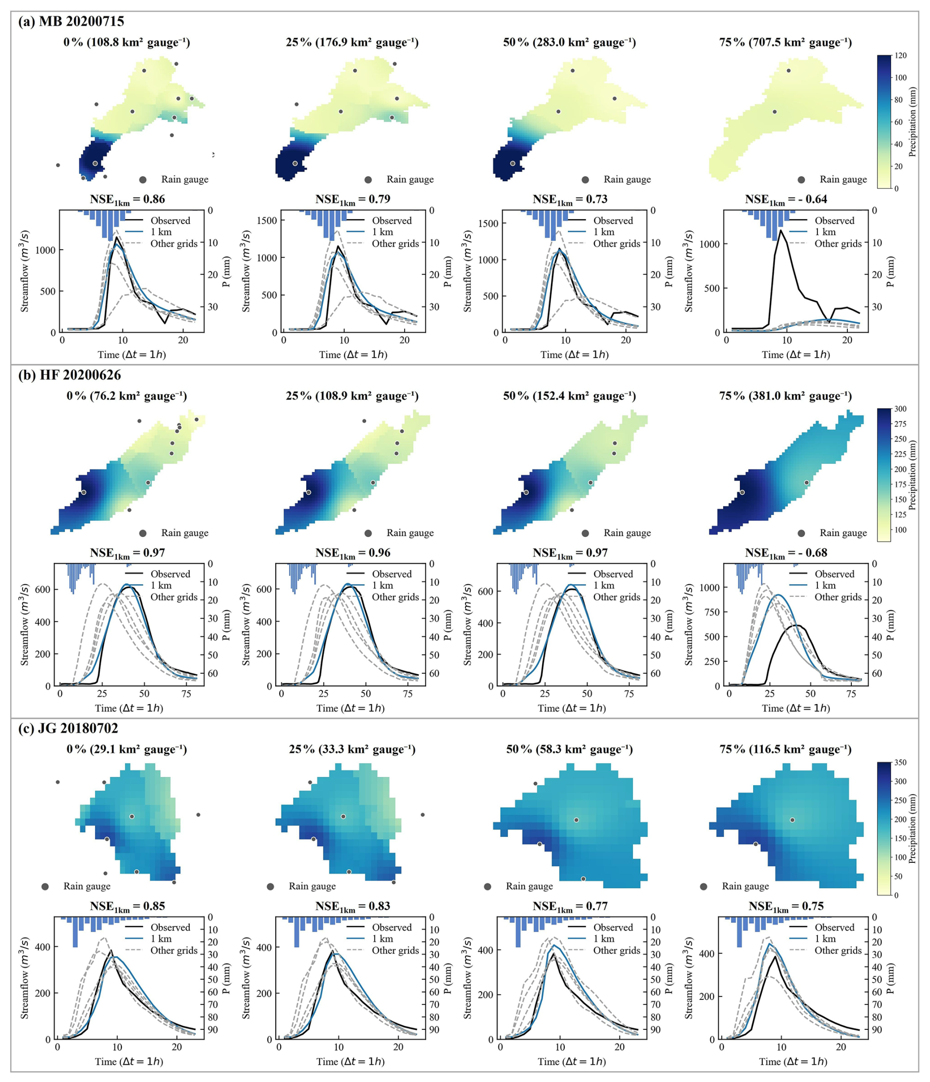
Figure 14 Effects of rainfall station density on rainfall spatial distribution and flood simulation performance under different spatial resolutions.

5 Conclusions

To investigate the influence of spatial resolution on flood-simulation accuracy in large river basins, this study developed the GDHF model for the Jialing River basin at five resolutions: 1, 3, 5, 10 km, and sub-watershed. An XGBoost model was then used to identify key flood characteristics that govern the choice of spatial resolution. Based on these results, the study determined the optimal spatial resolution for different flood-characteristic ranges and further examined how rainfall station density constrains the benefits of spatial refinement. The main conclusions are as follows:

1. Multi-resolution simulations show that the 1 km grid consistently performs best, with NSE > 0.80 at all stations, | BIAS | and | RPE | around 10 % and 15 %, respectively, and | PTE | < 5 h. However, for stations controlling large drainage areas, additional spatial refinement yields only marginal accuracy gains. In contrast, for small- and medium-sized watersheds, finer grids substantially improve the representation of runoff generation and routing processes.

2. XGBoost results indicate that Area is the dominant factor governing improvements in IMP_NSE. Rainfall characteristics (P_sum, P_max, R_cv) strongly influence improvements in IMP_NSE, IMP_BIAS, and IMP_RPE, while underlying-surface properties (P_a, Slope, Clay, Elev, R_res) also affect the extent of accuracy gains. These factors exhibit pronounced nonlinear impacts on model improvement.

3. Optimal-resolution statistics show that fine grids (1–3 km) offer substantial benefits only when flood processes exhibit strong nonlinearity – such as in small basins, gentle slopes, or low-rainfall conditions. For larger basins or weakly nonlinear floods, performance differences across spatial resolutions diminish, and further refinement provides little added value.

4. The advantages of fine grids are limited by the spatial representativeness of rainfall inputs: as rainfall station density decreases, the benefits of spatial refinement weaken or even disappear. Thus, increasing spatial resolution alone cannot offset errors arising from insufficient rainfall observations.

Appendix A

A1 Rainfall

This study selected the indicators P_max, P_sum, P_avg, η, and R_cv to describe the magnitude, intensity, and spatiotemporal distribution of rainfall during flood events. Except for η, the remaining indicators are computed as watershed-averaged values for each individual flood event. The maximum rainfall intensity P_max is defined as the maximum value of watershed-averaged rainfall:

$$\begin{array}{}\text{(A1)}& P_{\max }=max\left(\stackrel{\mathrm{‾}}{P}\left(t\right)\right)\end{array}$$

Where $\stackrel{\mathrm{‾}}{P}\left(t\right)$ represents the watershed-averaged rainfall at each time step t (mm), calculated using the Thiessen polygon method.

The total rainfall P_sum and the average rainfall intensity P_avg represent the total rainfall and the average rainfall over all time steps, respectively (Zhou et al., 2021):

$$\begin{array}{}\text{(A2)}& {\displaystyle }{P}_{\mathrm{sum}}={\sum }_{t=\mathrm{1}}^T\stackrel{\mathrm{‾}}{P}\left(t\right)\text{(A3)}& {\displaystyle }{P}_{\mathrm{avg}}={\displaystyle \frac{\mathrm{1}}{T}}{\sum }_{t=\mathrm{1}}^T\stackrel{\mathrm{‾}}{P}\left(t\right)\end{array}$$

The rainfall spatial non-uniformity coefficient η and the temporal variation coefficient R_cv (Wang et al., 1999) are used to describe the spatiotemporal distribution characteristics of rainfall:

$$\begin{array}{}\text{(A4)}& {\displaystyle }\mathit{\eta }={\displaystyle \frac{P_{\mathrm{avg}}}{P_{\max ,i}}}\text{(A5)}& {\displaystyle }\mathit{\mu }={\displaystyle \frac{\mathrm{1}}{T}}{\sum }_{t=\mathrm{1}}^T{P}_t\text{(A6)}& {\displaystyle }\mathit{\sigma }=\sqrt{{\displaystyle \frac{\mathrm{1}}{T-\mathrm{1}}}{\sum }_{t=\mathrm{1}}^T(P_t-\mathit{\mu }{)}^{\mathrm{2}}}\text{(A7)}& {\displaystyle }{R}_{\mathrm{cv}}={\displaystyle \frac{\mathit{\sigma }}{\mathit{\mu }}}\end{array}$$

where P_max,i represents the maximum point rainfall in the watershed (mm); μ and σ represent the mean and standard deviation of rainfall intensity, respectively.

A2 Underlying Surface

The underlying surface indicators include antecedent precipitation (P_a) and soil texture components (sand, silt, and clay fractions). For sand, silt, and clay fractions, the value for each grid cell is taken as the average value over the statistical grid, and the sum of the three fractions equals 1. The antecedent precipitation P_a quantifies the soil moisture condition prior to a rainfall event and can be used to analyze the watershed's nonlinear response and the runoff generation process (Schoener and Stone, 2019):

$$\begin{array}{}\text{(A8)}& P_{\mathrm{a},t}=K_{\mathrm{a}}\left(P_{a,t-\mathrm{1}}+P_t\right)\end{array}$$

where P_a,t is the antecedent precipitation on day t, P_t is the rainfall on the same day, and K_a is the decay coefficient.

A3 Watershed

Watershed indicators include R_res, Area, Shape, Slope, and Elev. These indicators characterize the topographic features and storage conditions of the watershed (Ma et al., 2021). R_res represents the total reservoir retention capacity within the watershed, calculated as the sum of the capacities of all reservoirs in the watershed. Area represents the total area of the watershed. The watershed shape factor (Shape) is defined as the ratio of the Area to the square of the main axis length L_axis of the watershed.

$$\begin{array}{}\text{(A9)}& \mathrm{Shape}={\displaystyle \frac{\mathrm{Area}}{L_{\mathrm{axis}}^{\mathrm{2}}}}\end{array}$$

Watershed average slope (Slope) and average elevation (Elev) are calculated using DEM data. The gradient of each DEM grid cell within the watershed is computed, where $\frac{\partial z}{\partial x}$ and $\frac{\partial z}{\partial y}$ represent the rate of change of elevation in the x and y directions for each cell.

$$\begin{array}{}\text{(A10)}& \mathrm{Slope}=\arctan \sqrt{{\left({\displaystyle \frac{\partial z}{\partial x}}\right)}^{\mathrm{2}}+{\left({\displaystyle \frac{\partial z}{\partial y}}\right)}^{\mathrm{2}}}\end{array}$$

Appendix B

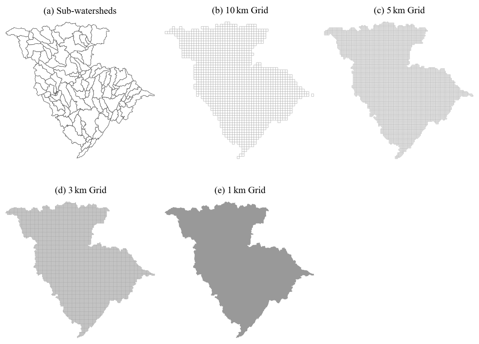
Figure B1 Sub-watershed and 10, 5, 3, and 1 km grid divisions of the study area.