Integrating topographic continuity and lake recession dynamics for improved bathymetry mapping from DEMs

Accurate lake bathymetry is critical for advancing hydrological and biogeochemical research, yet large-scale and deep-water mapping remains constrained by cost challenges. While remote sensing techniques have been extensively employed for bathymetric mapping, their effectiveness is primarily limited to shallow waters due to the rapid attenuation of optical signals with increasing depth. To overcome this limitation, we propose a novel bathymetric mapping method that leverages topographic continuity to infer underwater terrain by simulated progressive lake recession. This approach relies solely on Digital Elevation Model (DEM) data, using shoreline topographic gradients to estimate depth, providing a robust alternative for regions where conventional surveying is impractical. Validation across 12 lakes on the Tibetan Plateau demonstrated promising accuracy, with an average normalized root-mean-square error of 19.08 % for depth estimation and a mean absolute percentage error of 23.47 % for lake water storage. To evaluate the method's generalizability across diverse hydrological settings, it was applied to Lake Mead in the United States, producing a bathymetric map with a correlation coefficient of 0.66 with in situ measurements. Overall, this study introduces a low-cost solution for bathymetric mapping in data-scarce regions, offering a valuable tool for assessing lake water storage at regional and global scales.

1 Introduction

Lakes, covering approximately 2 % of the global land surface, play a critical role in water resource assessments and water balance analyses (Råman Vinnå et al., 2021; Pekel et al., 2016). They act as essential mediators of water-energy exchanges and serve as sensitive indicators of climate change at both regional and global scales (Vinogradova et al., 2025). By directly influencing water resource equilibrium, lakes are integral to hydrological and ecological processes (Williamson et al., 2009). Lake bathymetry and volume, two key physical characteristics of lakes, are fundamental for various applications, including hydrodynamic modeling (Yoon et al., 2012; Durand et al., 2008), aquatic vegetation monitoring (Gong et al., 2021), water resource management (Li et al., 2023; Yang et al., 2021), and climate model evaluation (Woolway et al., 2020). Therefore, accurate measurements of lake depth and water storage are essential for environmental conservation and sustainable resource management. However, the efficiency of current bathymetric mapping technologies remains limited, substantially compromising the accuracy of lake water storage estimates and restricting their practical applications. This underscores an urgent need for methodological innovations to advance lake depth estimation and water storage prediction.

Traditional in situ bathymetric surveys rely on shipborne echo sounders, airborne LiDAR, and optical imaging sensors (Guo et al., 2022; Song et al., 2014; Smith and Sandwell, 1997). While these techniques provide high-resolution data, they are costly and impractical for large-scale lake assessments. Satellite remote sensing offers a cost-effective alternative for global inland water monitoring (Li et al., 2021b; Sheffield et al., 2018), yet accurately mapping underwater topography remains a significant challenge. Optical remote sensing is widely used for bathymetric mapping in shallow waters (Wang et al., 2024), but its effectiveness declines exponentially in deeper lakes due to limited light penetration (Roy and Das, 2022). Radar altimetry and Digital Elevation Models (DEMs) can capture topographic features but exhibit fundamental limitations in characterizing submerged terrain. Notably, prevailing global DEM products assign a fixed elevation value to water-covered areas, reflecting surface elevation rather than actual underwater topography (Li et al., 2021a; Yamazaki et al., 2017; Farr et al., 2007). Therefore, these products depict submerged terrain only in areas inundated after the observation period, thereby failing to provide a comprehensive representation of the lake bathymetry.

In recent years, the integration of satellite altimetry and optical remote sensing data has been increasingly employed to monitor the depth of inland waters (Li et al., 2019; Qiao et al., 2019; Duan and Bastiaanssen, 2013). Lake surface areas are typically derived from optical imagery, while water surface elevations are obtained from satellite altimetry data (Li et al., 2021a). By correlating lake area time series with corresponding elevation measurements, area-elevation relationships can be established (Luo et al., 2021; Gao, 2015). Based on these relationships, lake water storage is estimated using geometric calculation formulas tailored to specific lakes. For instance, Li et al. (2020) combined multi-source satellite altimetry data with Landsat imagery to establish area-elevation relationships, which were subsequently utilized to estimate dynamic reservoir depths. They further employed an extrapolation method to generate a complete bathymetric dataset. Although this method enables comprehensive bathymetric mapping, it depends on prior knowledge of the maximum lake depth as a constraint, limiting its applicability in regions where such information is unavailable.

Shoreline topography plays a crucial role in determining lake depth (Messager et al., 2016; Pistocchi and Pennington, 2006), as shoreline morphology and slope significantly impact water flow and sedimentation processes (Edmonds and Slingerland, 2010). Therefore, lake shoreline characteristics provide valuable input for estimating lake depth. Some studies have employed statistical models to analyze large datasets of known lake and reservoir depths. Nonlinear models based on surrounding topography have been developed to estimate average or maximum water depth, which is then used to calculate lake water storage (Han et al., 2024; Cael et al., 2017; Messager et al., 2016). While such methods are generally reliable for large-scale studies due to the compensatory effects of under- and over-estimation, uncertainties and biases remain substantial at the local or individual lake scale. Alternative approaches suggest that lake bathymetry can be inferred by extrapolating or interpolating from the surrounding terrain (Liu and Song, 2022; Getirana et al., 2018). Although these approaches can partially reconstruct underwater topography and estimate water storage, they often require prior in situ data, such as maximum lake depth, to constrain the results. Recently, several methods have been developed that eliminate the need for field measurements (Han et al., 2024; Fang et al., 2023; Zhu et al., 2019). Due to sediment accumulation, most modern lakes tend to develop deep-water zones with relatively flat bottoms (Zhang et al., 2018). Current DEM-based bathymetric mapping methods often truncate predictions when the estimated depth exceeds measured values (Zhang et al., 2016), leading to artificially flattened lake bottoms. However, such truncation fails to account for sedimentation processes and variations in underwater topography resulting from sediment accumulation.

To address these limitations, this study proposes a novel three-dimensional bathymetric mapping approach that utilizes DEM data to estimate lake depth and water storage. The method leverages shoreline geometric features and topographic factors extracted from DEMs, while explicitly accounting for the physical processes of lake level recession (used here solely as a physical simulation in the reconstruction procedure, rather than implying an observed lake level trend) and sediment deposition. By capturing the reshaping effects of sediment accumulation on lakebed morphology, this approach provides a more accurate representation of underwater topography and supports improved estimates of lake water storage. Consequently, it offers a promising solution for generating bathymetric maps and estimating lake water storage in natural lakes, even in regions with limited in situ data.

2 Data and Methods

2.1 Data

2.1.1 Digital Elevation Model datasets

NASADEM, an enhanced version of the Shuttle Radar Topography Mission (SRTM) DEM with a 1 arcsec (∼ 30 m at the equator) spatial resolution, was used as the primary input dataset (Crippen et al., 2016). One of its key advantages for bathymetric mapping is its early acquisition time, which captures more exposed shoreline areas. Consequently, the DEM preserves geomorphic information from historically exposed shorelines and shallow lake margins, providing critical physical constraints for reconstructing present-day underwater topography and enabling more comprehensive lake depth estimation. It has been reprocessed using advanced algorithms to refine the original SRTM radar signal, incorporating precise elevation benchmarks primarily from the Ice, Cloud, and Land Elevation Satellite (ICESat) Geoscience Laser Altimeter System (GLAS) and the Advanced Spaceborne Thermal Emission and Reflection Radiometer (ASTER). Validation studies across the Tibetan Plateau have confirmed its high vertical accuracy, with a low root-mean-square error (RMSE) of 3.36 m in the validation area (Li et al., 2022). This dataset is publicly available through NASA's Earthdata portal (https://www.earthdata.nasa.gov, last access: 30 April 2026). To assess the impact of input data with different spatial resolutions on the simulation results, we incorporated two additional datasets: ALOS PALSAR DEM (12.5 m spatial resolution) and MERIT DEM (3 arcsec resolution, ∼ 90 m at the equator). The ALOS PALSAR DEM data were obtained from the Japan Aerospace Exploration Agency (JAXA, https://www.eorc.jaxa.jp, last access: 30 April 2026), and the MERIT DEM data were sourced from the International Centre for Water Hazard and Risk Management (ICHARM, https://hydro.iis.u-tokyo.ac.jp, last access: 30 April 2026). Since the proposed method relies on pixel-wise calculations and involves area estimation, all spatial data were processed using the Albers equal-area projection to ensure consistency and reliability. The geographic coordinate system of the Tibetan Plateau lake data is WGS84, whereas that of the Lake Mead data is NAD83.

2.1.2 In situ bathymetric data

The in situ data were provided by the National Tibetan Plateau/Third Pole Environment Data Center (http://data.tpdc.ac.cn, last access: 30 April 2026), which were collected using an echo sounder (Lowrance HDS5). Spatial interpolation was performed at a 30 m resolution, utilizing bathymetric points with longitude, latitude, and depth to generate in situ bathymetric maps. Shoreline shapefiles were extracted at the zero-depth boundary (depth = 0 m) from in situ measurements and used to calculate lake surface areas (Fig. S1 in the Supplement). The selected lakes, which are evenly distributed across the Tibetan Plateau (Fig. 1), exhibit diverse morphologies (Fig. S2). Their mean water surface elevations range from 4299 to 5171 m, spanning an altitude difference of approximately 1000 m. Most lakes have surface areas between 90 and 500 km², except for Siling Co, which is significantly larger at approximately 2400 km². Maximum lake depths range from 4 to 130 m, reflecting diverse bathymetric features and shoreline complexities. Detailed lake characteristics are presented in Table 1. Additionally, to assess the method's applicability across disparate hydrological contexts, a 30 m resolution bathymetric map of Lake Mead – an artificial reservoir – was obtained from the United States Geological Survey (USGS, https://www.usgs.gov/, last access: 30 April 2026). This dataset includes information on post-impoundment sediment distribution within the lake. However, due to the limited coverage of the in situ bathymetric map, portions of the eastern region of Lake Mead were excluded from the analysis.

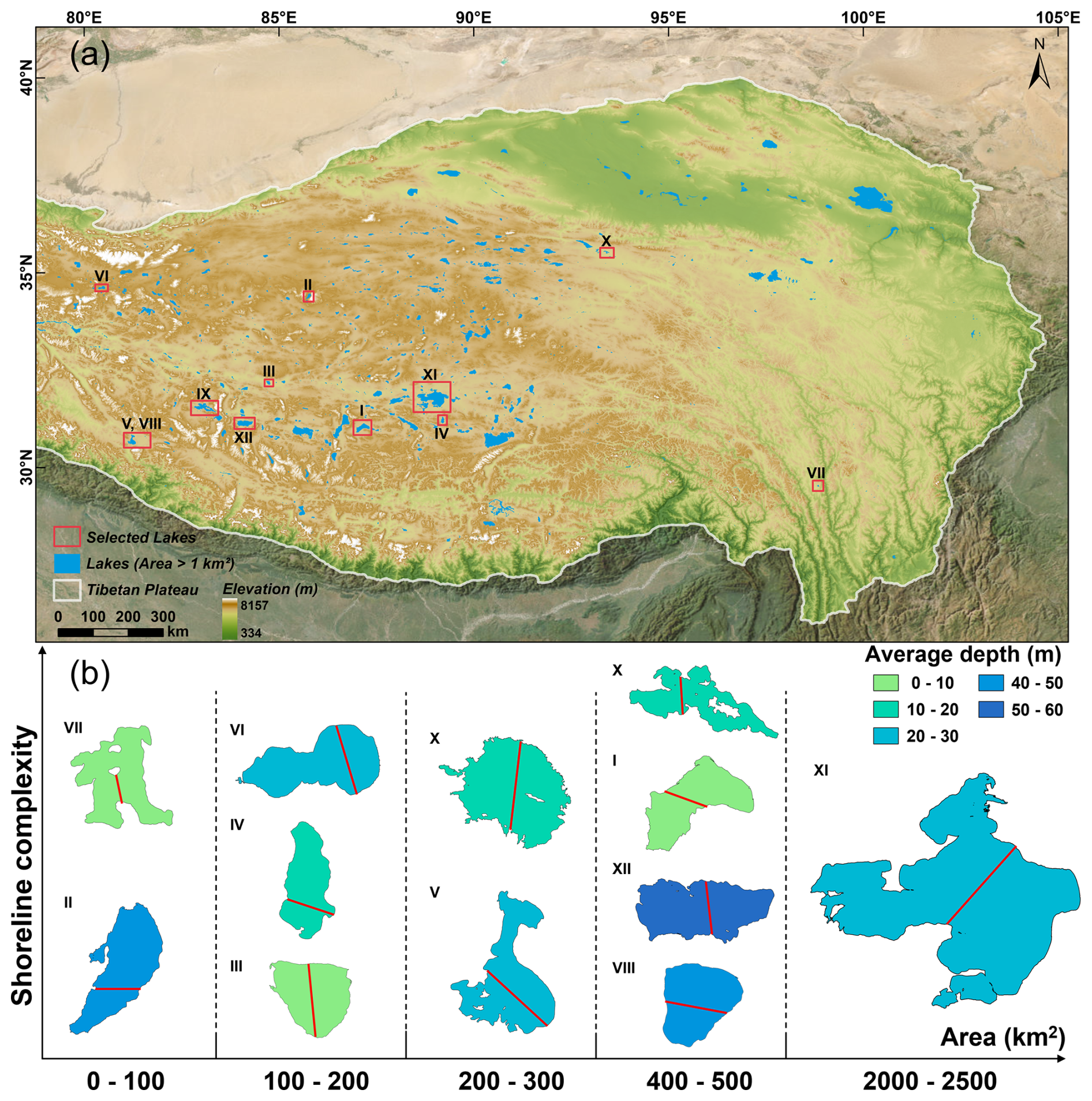
Figure 1 Overview of the 12 sample lakes on the Tibetan Plateau. (a) Distribution of lakes larger than 1 km² across the Tibetan Plateau, with the sample lakes in this study highlighted by red rectangles. (b) Shape characteristics of the 12 sample lakes, with colors indicating differences in mean lake depth. The red line denotes the transect used for validation in Fig. 8.

Table 1 Overview of the sample lakes on the Tibetan Plateau.

2.1.3 Comparative datasets

The estimated lake water storage values were compared with those reported in three previous studies. GLOBathy is a recently developed global dataset that generates bathymetric maps based on maximum depth estimates, combined with the geometric and physical properties of water bodies from the HydroLAKES dataset (Khazaei et al., 2022). Han et al. (2024) adopted an improved grid-based photon noise removal method to extract underwater photon signals from ICESat-2 data. By integrating statistical modeling with self-affine theory, they generated bathymetric maps of lakes and estimated lake water storage for lakes larger than 0.01 km² on the Tibetan Plateau. Fang et al. (2023) employed a trigonometric function as the fundamental shape of depth profiles and applied error correction based on different water level elevations to reduce the impact of sediment layers on simulation accuracy. The method was applied to 12 lakes on the Tibetan Plateau, and the results were included in the comparison.

2.2 Method

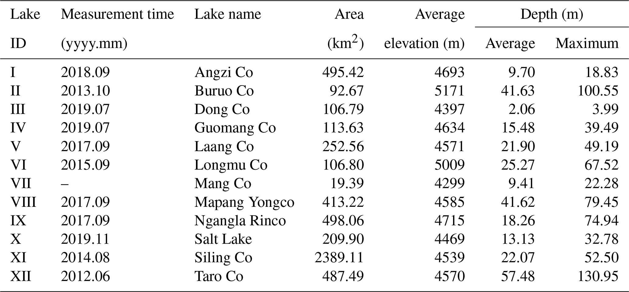
The bathymetric mapping algorithm consists of three main steps (Fig. 2). Parameter initialization: Key input parameters for underwater elevation estimation, including the water mask and shore slope, are extracted from the updated SRTM Water Body Data (SWBD) and the NASADEM elevation bands. The water mask defines the spatial extent of the computation, while the shore slope serves as the independent variable for estimating underwater elevation. To better capture the representative shore-to-lake gradient, we estimate shore slope using a directional and robust scheme. Directional slopes are first computed along multiple orientations (eight-neighbor directions) and then rescaled within the buffer zone to match the magnitude range of a conventional 3 × 3-window slope map, thereby preserving directionality while reducing biases associated with single-direction calculations. Underwater elevation calculation: The water mask is treated as the initial lake surface. A simulated recession process is then applied, progressively lowering the water level and reducing the water mask coverage. This simulation process, initially proposed by Zhu et al. (2019), has been applied in recent studies. However, previous studies require manual predefinition of the water level drop at each step. In this study, the process is improved to automatically simulate the entire recession without manual intervention. A detailed description of the simulation process is provided in Sect. 2.2.2. At each step of the simulated retreat, elevation values for newly exposed underwater pixels are calculated. These elevations are estimated using a new profile-based underwater elevation model. This model adopts a quadratic function as the base form and defines an assumed lowest point based on the relative slopes of the two banks. Closed-form expressions then describe slope and elevation variations on both sides of this point, remaining applicable throughout the iterative drawdown. This iterative process continues until all pixels within the original water mask are assigned updated elevation values. Consequently, the original water surface elevations in the DEM are progressively replaced with estimated underwater elevations. Lake water storage estimation: The updated DEM, containing elevation values for underwater pixels, is combined with the lake extent to generate a complete bathymetric map. From this map, lake depth and water storage are calculated. This structured approach ensures accurate bathymetric mapping by iteratively estimating underwater elevations from shoreline topography and water level recession.

Figure 2 Flowchart of bathymetry generation and lake water storage estimation.

2.2.1 Parameter initialization

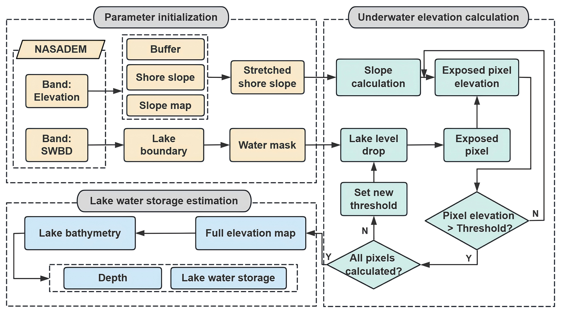
The DEM dataset used in this study assigned the lake surface elevation to all water-covered pixels. To distinguish water bodies from surrounding land areas, a binary land-water classification is generated by filtering the SWBD band in the DEM, with pixels set to 255 denoting water. As the initial classification may contain fragmented water patches, a connected component detection algorithm is applied to eliminate these artifacts. Only the largest connected region is considered the main lake body. Once the main lake body is identified, an edge detection algorithm is employed to extract shoreline pixels. A new matrix – referred to as the water mask matrix – is then generated with the same spatial reference as the input DEM (Fig. 3b).

Figure 3 Shoreline slope estimation process for LBD. (a) Multi-level buffer zones surrounding the lake boundary. (b) Slope calculation using linear regression within the buffer zone. The red pixel indicates the target shoreline pixel under calculation, while the red boxes represent the surrounding pixels involved in the calculation. (c) Linear fitting process in a specific direction, with the red line representing the fitted slope.

A multi-level buffering strategy is employed to define the spatial extent of the DEM used in subsequent calculations (Fig. 3a). A maximum buffer zone of 600 m (approximately 15–20 pixels) is established around the lake boundary in the DEM (LBD). Within this zone, nested buffer zones are generated at 100 m intervals (about 3–4 pixels). The average elevation within each buffer is calculated, yielding a series of elevation values that increase with distance from the LBD.

A terrain transition point is identified by progressively sampling outward from the LBD to determine where the elevation trend shifts from increasing to decreasing. The edge at this transition point is defined as the outer edge of the final buffer extent, thereby ensuring that only terrain relevant to shoreline slope estimation is included. If no transition point is detected, the default buffer of 600 m is used.

Elevation values within the final buffer zone are used to estimate the initial shore slope. As illustrated in Fig. 3b, for each lake boundary pixel in the water mask matrix, an 8-neighborhood detection method is applied to identify adjacent land pixels in the landward direction. Using the DEM's elevation band, elevation values are extracted along this landward direction within the buffer zone (Fig. 3c). A linear or polynomial regression is then applied to estimate the slope. Once all landward slopes are computed, their average value is used as the initial shore slope, which serves as a key input for underwater elevation estimation. This process is repeated for all LBD pixels.

While the computed shore slope accounts for local terrain orientation, relying solely on a linear regression within a fixed window may not fully capture the elevation variability within the buffer zone. To better represent the general terrain transition from the shoreline toward the lake center, the method integrates the directional shore slope with broader topographic variation observed across the entire buffer zone. A slope map of the buffer zone is generated by applying a 3 × 3 moving window to estimate the slope at each pixel. This approach captures localized terrain undulations and provides a more comprehensive representation of elevation variation within the buffer. To enhance statistical robustness and reduce the influence of extreme values, outliers in the slope data are removed using a 95th-percentile threshold. The previously computed directional shore slope values are then rescaled to match the value range of the slope map using the following transformation formula:

$$\begin{array}{}\text{(1)}& \begin{array}{rl}{S}_{\mathrm{1}}^{\prime }\left(ij\right)=& min\left(S_{\mathrm{2}}\right)+{\displaystyle \frac{S_{\mathrm{1}}\left(i,j\right)-min\left(S_{\mathrm{1}}\right)}{max\left(S_{\mathrm{1}}\right)-min\left(S_{\mathrm{1}}\right)}}\\ & \times \left(max\left(S_{\mathrm{2}}\right)-min\left(S_{\mathrm{2}}\right)\right).\end{array}\end{array}$$

2.2.2 Underwater elevation calculation

Based on the principle of terrain continuity, underwater areas closer to the shoreline tend to exhibit greater similarity to the topographic characteristics of the shoreline. Following this principle, the elevation values of underwater pixels near the shoreline are iteratively estimated using the following formula:

$$\begin{array}{}\text{(2)}& h_i=h_i^{\prime }-d\cdot k_i,\end{array}$$

where h_i represents the elevation of the ith pixel, $h_i^{\prime }$ is the elevation of the adjacent land pixel, d is the distance between the two pixels, and k_i is the slope at the location of the ith pixel. As shown in Eq. (2), calculating the elevation of the ith pixel requires the known elevation value of a neighboring pixel (i.e., $h_i^{\prime }$) as input. Therefore, the sequence and pattern of underwater elevations used in the calculations significantly influence the final bathymetry results. This approach simulates the physical process of water level recession, gradually exposing underwater pixels. A loop-based method is then employed to iteratively calculate the elevation of these pixels following topographic gradients.

As illustrated in Fig. 4a, this process improves the simulation of lake recession. During each iteration, the lake level decreases incrementally, exposing a new set of underwater pixels. In steep regions, fewer underwater pixels are exposed per iteration due to rapid elevation changes, while in flatter areas, more pixels become exposed at once. As each pixel is exposed, its elevation is calculated sequentially, preserving spatial continuity and topographic consistency.

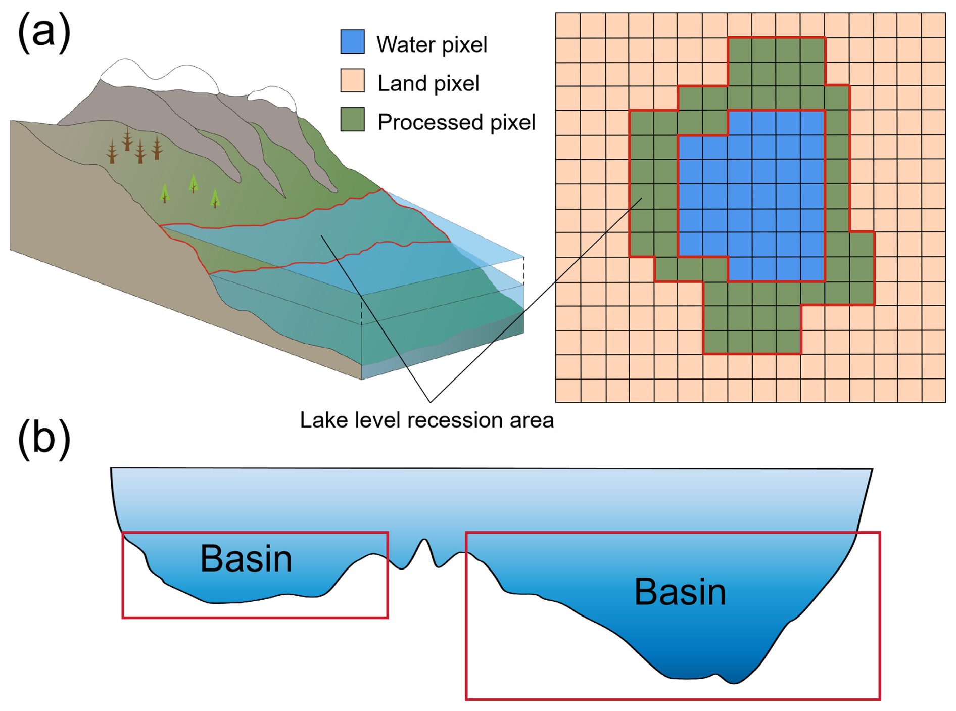
Figure 4 Simulation of the physical process of lake level recession. (a) Schematic illustration of lake level recession during bathymetric calculation, where the red lines represent the lake boundaries before and after each drop in water level. (b) Longitudinal profile of the lake along its central axis, with the red rectangle indicating the extent of the sub-basin.

The first iteration begins at the boundary of the water mask, where the elevations of all pixels adjacent to the shoreline are calculated. Among these newly computed pixels, the lowest elevation is identified and used as the threshold for the initial water-level drop. Once the elevation of an underwater pixel is determined, its status in the water mask is updated from water to land, indicating the transition from submerged to exposed. Following this, a new inner boundary is defined, and its elevation values are calculated. Pixels with elevation values greater than or equal to the updated threshold are retained for the next round of calculations. This iterative process continues until, within a given iteration, all calculated elevations are less than or equal to the threshold. At that point, the loop ends, and a new iteration begins with an updated threshold. With each iteration, the shoreline elevations become progressively more uniform, simulating a realistic recession of the water surface. The process repeats until no water pixels remain in the water mask, at which point the entire lake bottom is assigned elevation values, and the bathymetric computation is complete.

It is essential to recognize that the underwater topography of a lake cannot be simplified as a single basin, as multiple sub-basins may exist (Fig. 4b). Therefore, in this study, no constraints are imposed during the simulation of lake recession. Once newly exposed land pixels connect to the shoreline, the lake is segmented into multiple sub-basins. The recession process is then applied to each sub-basin individually through boundary detection. This approach avoids the oversimplified assumption that all lakes consist of a single basin and instead accurately captures the true complexity of lakebed morphology.

During the calculation process, most water pixels are adjacent to multiple land pixels, resulting in multiple potential elevation estimates for each water pixel. To determine the most reliable elevation, a weighted average operation is applied to the estimates from each direction. The weight for each direction is based on the distance from the water pixel to the opposite shore along that direction. The specific calculation formula is as follows:

$$\begin{array}{}\text{(3)}& \left\{\begin{array}{l}H=\sum _{i=\mathrm{1}}^n{H}_i\cdot w_i\\ w_i=\frac{\mathrm{1}/d_i}{{\sum }_{j=\mathrm{1}}^n\mathrm{1}/d_j}\end{array}\right.,\end{array}$$

where H represents the final calculated elevation of the water pixel, H_i represents the elevation estimate from direction i, w_i represents the weight assigned to direction i, d_i represents the distance from the water pixel to the opposite shore in direction i, and n represents the total number of directions with adjacent land pixels, d_j represents the distance from a water pixel to the opposite shore in direction j, used for normalization. The final elevation of each water pixel is determined as a weighted average of estimates from all valid directions. Under the assumption that pixels closer to the shoreline provide more reliable topographic information, elevation estimates associated with shorter distances to the shore are assigned higher weights.

In Eq. (2), the parameter k_i plays a crucial role in modeling underwater topography at each pixel. It reflects the lake's cross-sectional shape, and different assumptions about this shape can significantly affect simulation outcomes (Liu et al., 2020; Messager et al., 2016). For simplification, the method assumes that the lowest point along the lake's vertical profile could serve as the origin of a local coordinate system, as illustrated in Fig. 5. This lowest point typically lies closer to the steeper shore. To determine its position, shore slopes on both sides of the profile are first extracted. The assumed location of the lowest point is then calculated using the relative slopes of the two shores. Taking the left shore as an example, the horizontal distance between the lowest point and the left shoreline is determined by:

$$\begin{array}{}\text{(4)}& L=D_i\cdot {\displaystyle \frac{s_{\mathrm{r}}}{s_{\mathrm{l}}+s_{\mathrm{r}}}},\end{array}$$

where D_i is the total horizontal distance between the two shores along the current profile. s_l and s_r represent the slope values of the left and right shores, respectively. After determining the horizontal position of the lowest point, the model assumes that the slope at this point asymptotically approaches zero, representing a local minimum in the profile. Under this assumption, the slope at the ith pixel along the profile is assumed to decrease linearly with increasing distance from the shoreline. The slope variation is defined by the following formula:

$$\begin{array}{}\text{(5)}& k_i=s_{\mathrm{l}}\cdot \left(\mathrm{1}-{\displaystyle \frac{l}{L}}\right),\end{array}$$

where l represents the horizontal distance from the ith pixel to the left shore along the profile. Although Eq. (5) provides an initial estimate of the underwater topographic slope along the profile, continuous sedimentation gradually reshapes the lakebed, leading to a progressively flatter underwater terrain.

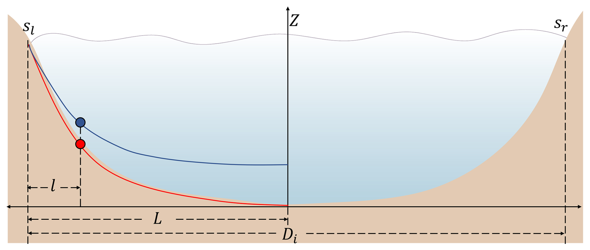
Figure 5 Schematic diagram of the lake profile coordinate system. The red line represents the lakebed profile before applying Eq. (6), while the blue line shows the profile after correction. The red and blue points indicate the positions of the calculation points along the profile before and after the correction, respectively.

To further enhance the simulation accuracy, a correction is introduced to account for sediment accumulation and its impact on underwater topography. It is assumed that sediment tends to accumulate more heavily with increasing distance from the shoreline, leading to a progressively flatter lake bottom (Håkanson, 1982). Incorporating this effect is expected to improve the realism of the simulation by aligning the modeled terrain with observed sedimentation patterns. The correction is applied to the initially estimated slope using the following formula:

$$\begin{array}{}\text{(6)}& k_i^{\prime }=k_i\times {\left({\displaystyle \frac{d_i}{D_i}}\right)}^{\mathit{\alpha }},\end{array}$$

where $k_i^{\prime }$ is the corrected slope at the ith pixel, and k_i is the uncorrected slope. d_i refers to the distance from the ith pixel on the current land boundary to the opposite shore along the profile. The exponent α reflects the influence of the surrounding terrain on sediment accumulation. To determine a representative value for α, we analyzed shoreline slope data from over 4000 lakes on the Tibetan Plateau using the HydroLAKES dataset. The resulting distribution (Fig. S3) indicates an average shoreline slope of approximately 5.14°, rounded to 5° as a reference threshold for assigning the value of α. The underlying assumption is that steeper shorelines facilitate greater sediment transport toward the lake center, resulting in the formation of flat sediment layers on the lakebed (Ju et al., 2012). Accordingly, to avoid overestimating the maximum depth in steep-shoreline lakes, α is determined as follows:

$$\begin{array}{}\text{(7)}& \left\{\begin{array}{ll}\mathit{\alpha }=\mathrm{1},& \mathrm{0}\mathit{°}<\stackrel{\mathrm{‾}}{\mathit{\theta }}\le \mathrm{5}\mathit{°}\\ \mathit{\alpha }=\mathrm{2},& \mathrm{5}\mathit{°}<\stackrel{\mathrm{‾}}{\mathit{\theta }}\end{array}\right.,\end{array}$$

where $\stackrel{\mathrm{‾}}{\mathit{\theta }}$ is the average slope within the defined buffer area, which is extracted during the “Parameter initialization” step. It should be noted that α is derived from lakes on the Tibetan Plateau and may therefore have regional limitations. When applying this method to other regions, the value of α should be adjusted according to local topographic and geomorphological conditions.

2.2.3 Lake water storage estimation

Following the underwater elevation calculation steps, a DEM representing the lake's underwater topography is generated within the extent defined by the water mask. It is important to note that this water mask is derived from the original DEM data and, therefore, reflects the lake boundary at the time the DEM was generated. To validate the accuracy of the simulated lake water storage results, we use the boundary (where depth is 0) from the measured data as the lake extent. The observed boundary is overlaid onto the simulated elevation map to generate a lake depth map, from which lake depth and water storage values are extracted. The formula used to estimate lake water storage is as follows:

$$\begin{array}{}\text{(8)}& V=\sum v_i=\sum s_i\times {\mathrm{depth}}_i,\end{array}$$

where V is the lake volume, v_i is the volume of the ith water pixel, s_i is the area of the ith pixel, and depth_i is the water depth at the ith pixel.

Since in situ bathymetric data did not include the water surface elevation at the time of measurement, a simple method was employed to extract this elevation. DEM elevation values along the observed lake boundary are extracted, and outliers are removed. The water surface elevation is then estimated by fitting the elevation distribution to a Generalized Extreme Value (GEV) distribution (Tseng et al., 2016; Morrison and Smith, 2002). Once the water surface elevation is obtained, the bathymetric map is converted to elevation values by subtracting the water depth from the water surface elevation.

2.2.4 Accuracy evaluation

To assess spatial differences between simulated and measured water depths, 2500 validation points were randomly selected across each lake's surface. A linear regression analysis using the least-squares method was conducted to examine the relationship between simulated depths and in situ measurements. The evaluation metrics included the Pearson correlation coefficient (r), the normalized root-mean-square error (NRMSE), and the mean absolute error (MAE). In addition, the difference between estimated and measured lake water storage was quantified using the percentage error (PE).

3 Results

3.1 Bathymetry mapping and lake water storage estimates

Three-dimensional visualizations of the simulated and in situ bathymetric maps (Fig. 6) were generated to compare their spatial patterns. The results demonstrate that the simulated bathymetry closely aligned with in situ water-depth measurements, accurately capturing variations in underwater terrain. Among all the sample lakes, Dong Co (Fig. 6c) exhibited the largest spatial discrepancy, likely due to its relatively flat shoreline, which limited the ability to infer underwater topographic patterns from the shoreline terrain. In contrast, Ngangla Rinco (Fig. 6i), with a more complex and fragmented shoreline, introduced localized inconsistencies in the simulated topography. As a result, the model tended to overestimate depths near the shore. Furthermore, as many salt lakes have expanded significantly in recent years, a noticeable discrepancy was observed between the in situ shoreline and the DEM-derived boundary. Therefore, the bathymetry near the shoreline – derived from the DEM in the transitional area between these boundaries – was observed to be less smooth than the in situ bathymetry.

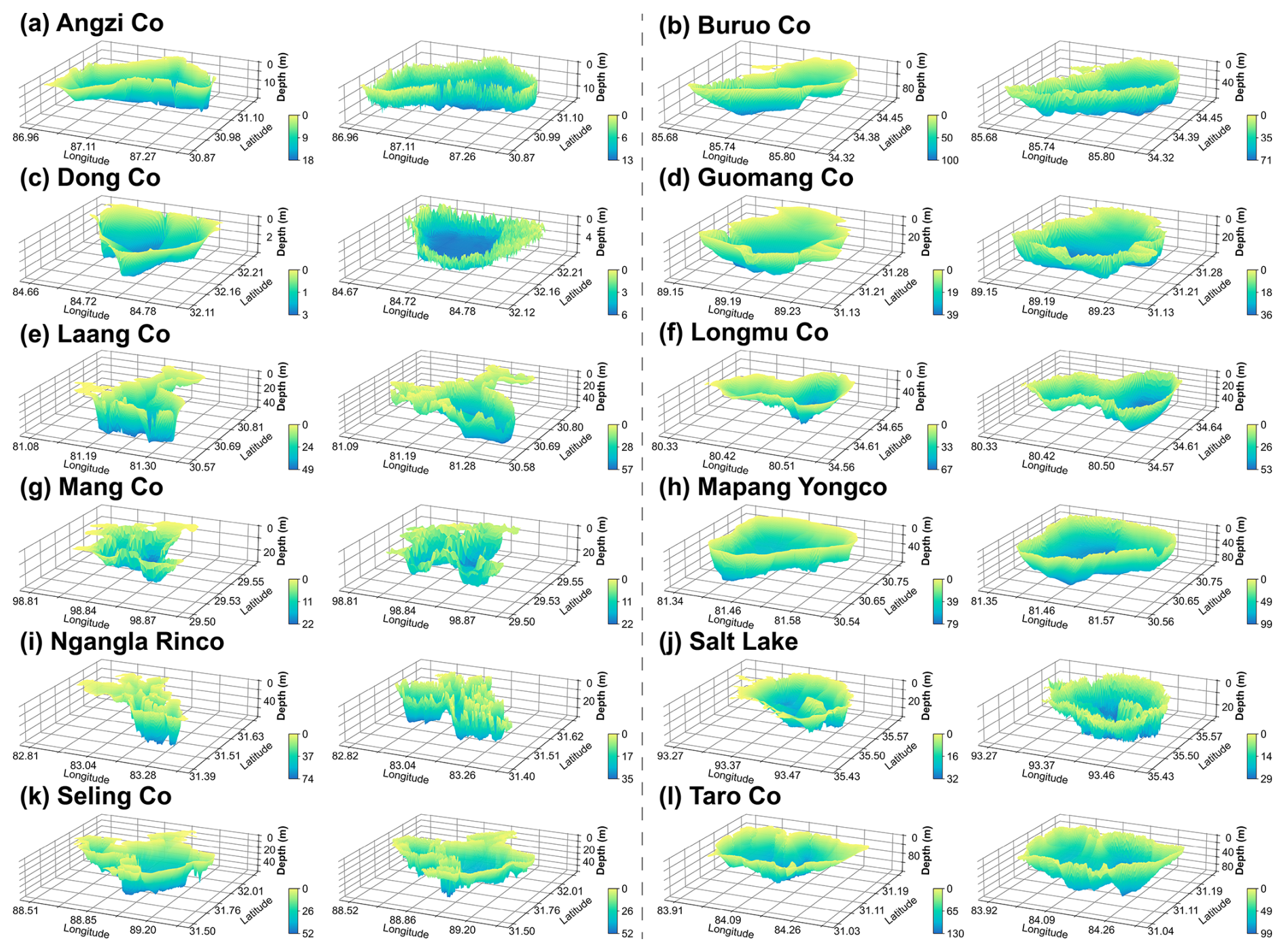
Figure 6 Three-dimensional bathymetric maps of the sample lakes derived from in situ measurements (columns 1 and 3) and the corresponding simulated results (columns 2 and 4).

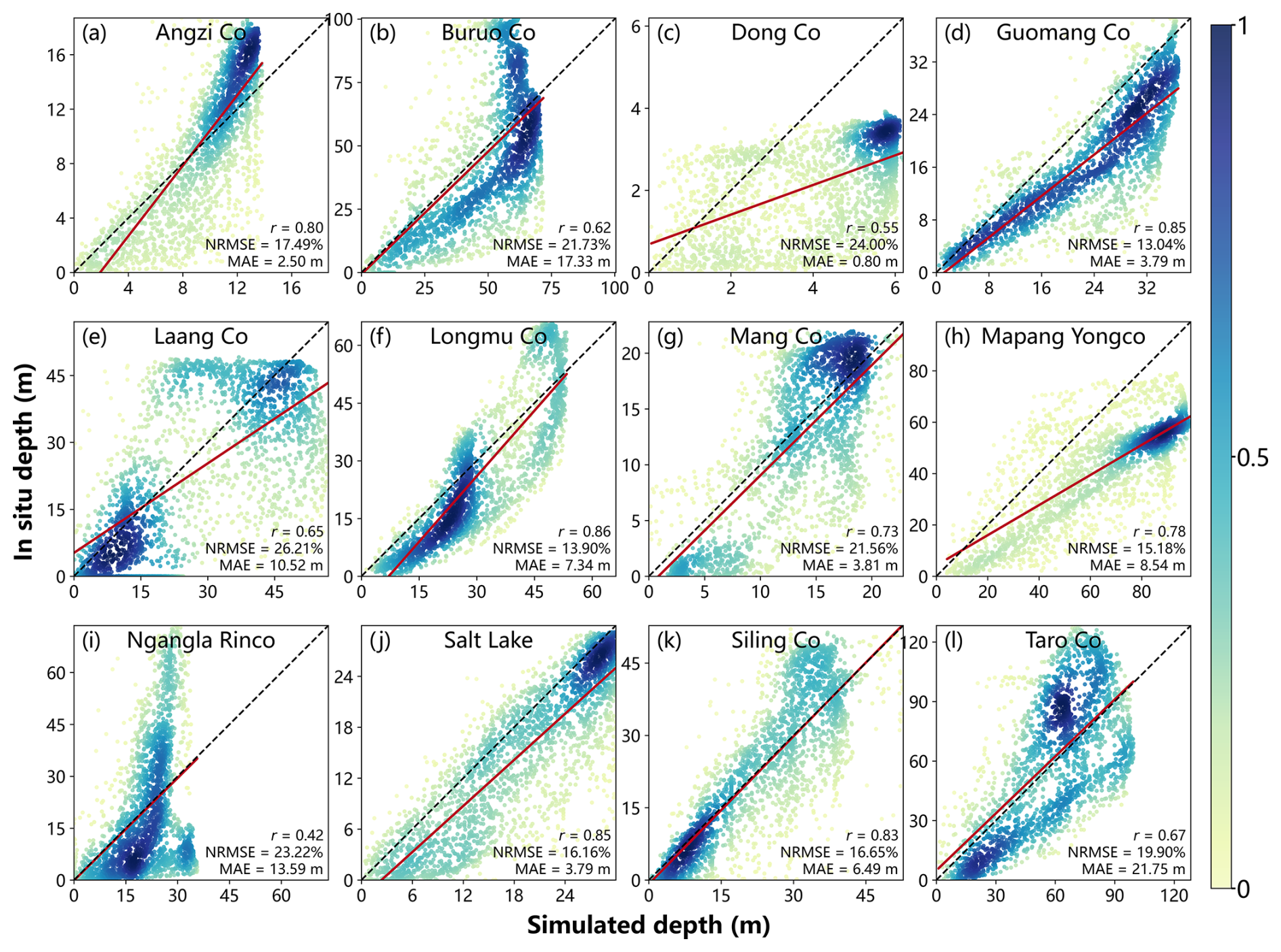
Figure 7 Scatter plots comparing simulated lake depths with in situ measurements. The dashed line indicates the 1 : 1 reference line, the red line represents the linear regression fit, and the point color denotes data density.

To quantitatively evaluate the accuracy of the simulated bathymetry, we randomly generated 2,500 validation points within each lake boundary and compared simulated depths against in situ measurements. As shown in Fig. 7, the simulated depths exhibit good agreement with observations, with an average r value of 0.72 and an average NRMSE value of 19.09 %. Because the method assumes that nearshore topography contains informative signatures of underwater slope structure, its performance depends on the signal-to-noise ratio (SNR) of shoreline-derived slope information and the degree of structural coupling between shoreline morphology and lakebed geometry within a basin.

Table 2 Comparison of maximum depth and lake water storage derived from in situ measurements and simulated bathymetric maps.

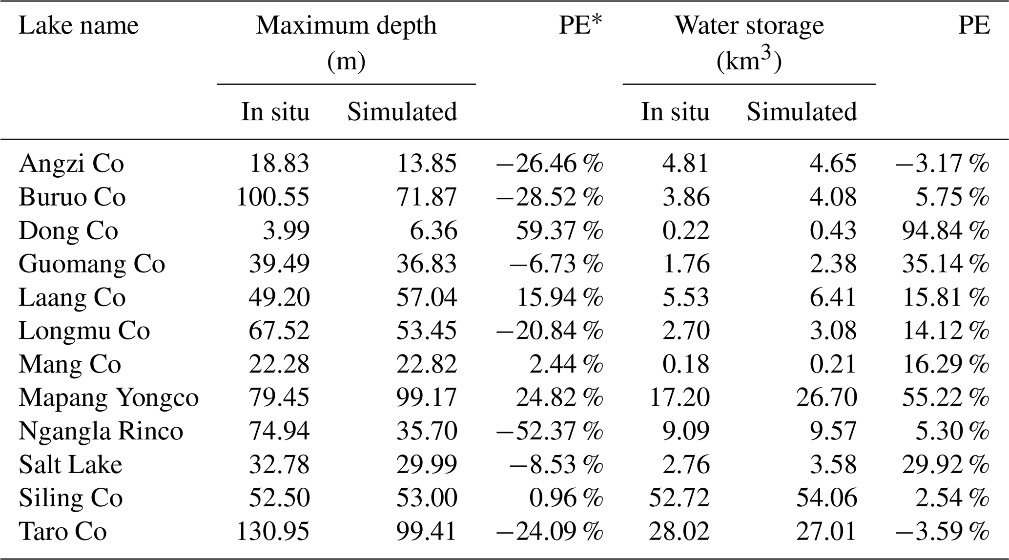
^∗ PE represents percentage error.

According to Table 2, the method underestimated maximum water depth for several lakes, including Angzi Co, Buruo Co, Longmu Co, Ngangla Rinco, and Taro Co. Among them, Ngangla Rinco (Fig. 7i) shows the weakest agreement. Inspection of the three-dimensional bathymetry (Fig. 6i) reveals an abrupt deepening in the southern part of the lake, indicating a localized bathymetric anomaly and partial shoreline–lakebed decoupling. Such features are difficult to infer from shoreline terrain alone, posing a challenge for approaches that rely primarily on nearshore topographic constraints. In contrast, simulated depths were overestimated for Dong Co and Mapang Yongco. In particular, Dong Co, with a surface area of 106.80 km² and a maximum depth of 3.99 m, exhibits relatively poor simulation performance despite its shallow depth. This likely reflects the limited depth range and the heightened influence of DEM noise and subtle topographic gradients, which can reduce the robustness of shoreline-derived slope signals and amplify relative errors.

Across all lakes, MAE is strongly correlated with lake depth (r=0.94). For deep lakes such as Buruo Co and Taro Co, where maximum water depths exceed 100 m, MAE values reached 17.33 and 21.15 m, respectively. This pattern suggests that shoreline–lakebed coupling tends to weaken with increasing depth, consistent with a reduced ability of shoreline-derived constraints to represent deep-basin morphology. Nevertheless, the model maintains acceptable accuracy across a wide range of lake sizes, depths, and morphologies, demonstrating its general applicability for regional-scale bathymetry estimation.

Lake water storage was calculated from the simulated bathymetric maps to further assess the effectiveness of the proposed method. For most lakes, the method yielded satisfactory water storage estimates (Table 2). The maximum water depth was derived as the maximum pixel value in the bathymetric map. It should be noted that in the simulated bathymetric maps, the location of the maximum depth pixel does not necessarily coincide with that in the in situ bathymetric map; nevertheless, the simulated deepest zone remains informative and provides a useful reference (Fig. S4). The PE between simulated and in situ bathymetric maps for Angzi Co, Buruo Co, Ngangla Rinco, Siling Co, and Taro Co remained within 10 %. Notably, despite a substantial underestimation of the maximum depth in Ngangla Rinco, its overall lake water storage estimate remained accurate. This result can be attributed to the offsetting effects between localized overestimation and underestimation in the simulated depth distribution. In contrast, Dong Co exhibited a large discrepancy in lake water storage estimates, with a PE of 94.84 % compared to the water storage derived from in situ bathymetry. This high error likely stemmed from the lake's shallow depth and small water storage, making it highly sensitive to even minor elevation errors. Despite the underestimation of maximum depth in Angzi Co, Buruo Co, Longmu Co, and Taro Co, the water storage estimates for these lakes remained reliable. This was because the overall depth distributions across the lake surface closely matched the in situ data, as illustrated in Fig. 7. In summary, among the 12 sample lakes, 10 exhibited water storage estimation errors below 30 %, including eight below 20 %, demonstrating that the proposed method performs well in most cases.

3.2 Validation of underwater terrain along transects

To assess the effectiveness of the proposed method for simulating underwater topography, Fig. 8 compares simulated and measured depth profiles along designated transects for 12 lakes. Each transect was carefully selected to align closely with the original depth survey routes while remaining near the lake center to ensure representative and consistent validation (Fig. S5). The average NRMSE across the 12 transects was 27.34 %, and the average MAE was 10.94 m, indicating an overall acceptable level of accuracy. In general, the simulated profiles were highly consistent with in situ measurements, effectively capturing the overall trends in depth variation. When transects extended toward lake shores, the simulated elevation gradients matched the in situ measurements well, demonstrating the method's capacity to represent shoreline-to-bottom topographic transitions accurately. However, deviations were observed near the lake bottoms in several cases. Simulated depths were overestimated in Angzi Co (Fig. 8a), Buruo Co (Fig. 8b), Mang Co (Fig. 8g), and Taro Co (Fig. 8l), while underestimations occurred in Dong Co (Fig. 8c) and Mapang Yongco (Fig. 8h). In other cases – such as Longmu Co (Fig. 8f), Ngangla Rinco (Fig. 8i), and Salt Lake (Fig. 8j) – although the general profile trends aligned well with observations, the method struggled to capture localized anomalies on the lake bottom. These discrepancies are likely linked to the complex geomorphological evolution of lakes on the Tibetan Plateau, which has experienced expansion, contraction, and migration processes over time. Such dynamic processes have resulted in heterogeneous sediment deposition and irregular bathymetric features (Yu et al., 2019). Consequently, a single correction formula may not fully account for the diverse morphologies of lakes. Despite these challenges, the proposed method demonstrates robust performance in simulating lake depth and bathymetry, supporting its applicability across varied lake environments.

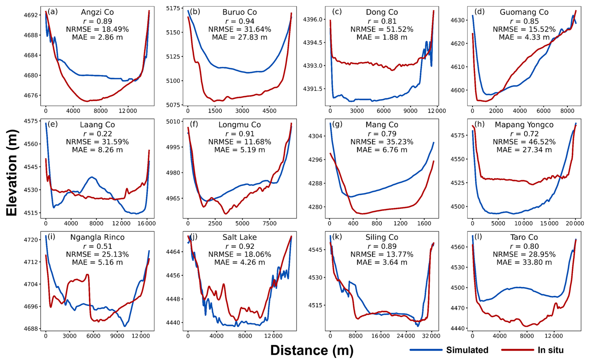
Figure 8 Elevation profiles along validation transects for each lake. Each transect was selected to closely follow the corresponding in situ survey route, providing representative comparisons between simulated and measured depths.

4 Discussion

4.1 Comparison with previous studies

The simulated lake water storage for the 12 sample lakes was compared with results from three previous studies (Table 3). For the GLOBathy dataset, absolute percentage error (APE) of lake water storage estimates ranged from 1.79 % to 324.93 %, indicating considerable variability, with nearly half of the lakes exhibiting errors greater than 50 %. In contrast, the dataset generated by Han et al. (2024) had an APE range of 0.52 % to 375.20 %, with four lakes showing APEs below 30 %. The large errors in GLOBathy are primarily attributed to limitations in its bathymetry reconstruction method and uncertainties in estimating maximum depth. Although Han et al. (2024) proposed an ICESat-2-based bathymetry reconstruction method, their dataset was derived from empirical equations. When applied to individual lakes, these equations can introduce unpredictable errors that may account for the observed inconsistencies. Moreover, among the nine overlapping sample lakes reported in Fang et al. (2023), the average APE was 31.80 %, outperforming both GLOBathy and Han et al. (2024). In comparison, our method achieved an average APE of 27.14 % across the same nine lakes. Furthermore, among all 12 sample lakes, only Dong Co, Guomang Co, and Mapang Yongco exhibited PEs greater than 30 %. These findings suggest that our method provides more accurate and robust lake water storage estimates compared to existing datasets.

Table 3 Comparison of percentage errors (PEs) in lake water storage estimates for the sample lakes across different studies.

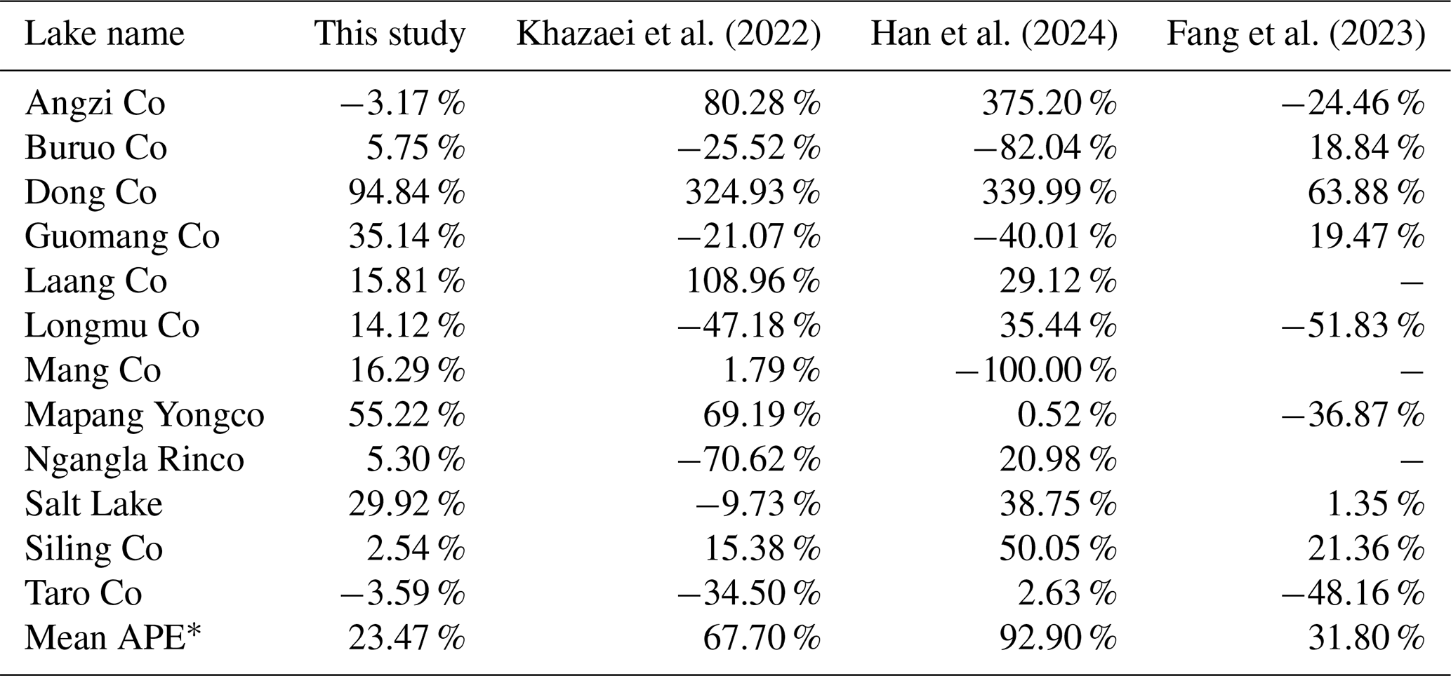
^∗ APE represents the absolute percentage error.

In the comparative analysis, as the water storage estimates from Han et al. (2024) were available only through 2022, the corresponding water surface extent and water level for that year were extracted, and the in situ water storage data were aligned to the same period for consistency. Since the water surface extent in GLOBathy's bathymetric maps was derived from HydroLAKES, the lake water storage estimates from GLOBathy were also adjusted to reflect the conditions in 2022. It should be noted that the boundary defined by the measured bathymetric data (depth = 0 m) was considered the lake shoreline in this study. Due to limitations in the bathymetric survey equipment, measurement uncertainties may exist within the recorded depth range.

4.2 Sensitivity to DEM resolution and buffer width

We evaluated the effects of different input DEM datasets on water depth simulation and found that the resolution and quality of the input data significantly affect the simulation performance (Fig. 9). Overall, simulations based on NASADEM achieved the lowest mean APE, followed by MERIT DEM and ALOS PALSAR. The detailed evaluation results for ALOS PALSAR and MERIT DEM are presented in Tables S1 and S2, respectively. In addition, the error distributions for NASADEM and MERIT DEM were more compact, indicating greater stability compared to the more dispersed errors observed in ALOS PALSAR-derived results. While increasing DEM resolution from 90 to 30 m clearly improved simulation accuracy, further refinement to 12.5 m using ALOS PALSAR unexpectedly reduced accuracy. Although recent studies have demonstrated the high vertical accuracy of ALOS PALSAR over the Tibetan Plateau (Xu et al., 2024), its performance in water depth simulation within our methodological framework was inferior to that of NASADEM. This discrepancy may be attributed to a combination of the intrinsic data quality and the simulation algorithm's sensitivity to varying spatial resolutions, which together could explain the suboptimal performance of ALOS PALSAR in this context. Beyond spatial resolution, the DEM acquisition time is also critical for our method. Because the algorithm infers underwater elevations from shoreline gradients and a DEM-derived water mask, DEMs acquired at lower lake levels can preserve more exposed nearshore topography. This additional geomorphic information strengthens constraints on shoreline-slope estimation and the subsequent recession simulation. In this regard, the earlier acquisition time of NASADEM may partly explain its better performance compared to ALOS PALSAR, despite the latter's finer spatial resolution.

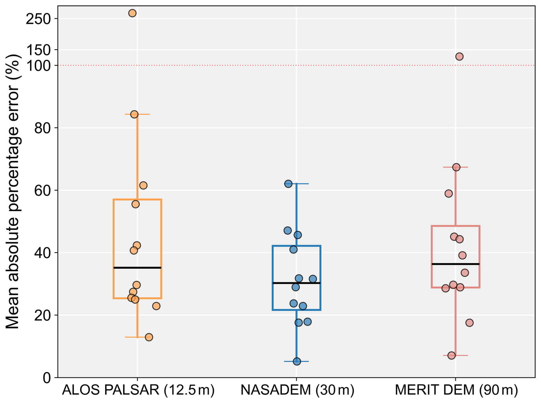
Figure 9 Box plots showing the distribution of mean absolute percentage error in lake depth simulations using three digital elevation models (DEMs) with varying spatial resolutions: ALOS PALSAR (12.5 m), NASADEM (30 m), and MERIT DEM (90 m). Each dot represents the mean absolute percentage error for an individual lake. Box ranges represent the upper and lower quartiles, and whiskers extend to 1.5 times the interquartile range. The original bathymetric survey points were selected as sample points for water depth. The data used for this figure are provided in Table S3.

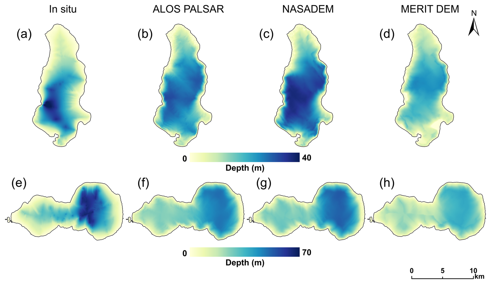
Figure 10 Comparison of simulated bathymetric maps generated using input DEMs with different spatial resolutions. Bathymetric maps for (a–d) Guomang Co and (e–h) Longmu Co were derived from in situ data, ALOS PALSAR (12.5 m), NASADEM (30 m), and MERIT DEM (90 m), respectively.

Table 4 Comparison of simulation results using input DEM data with different spatial resolutions.

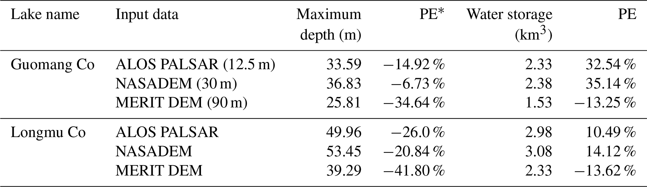
^∗ PE represents percentage error.

We compared simulated maximum depth and water storage for the 12 sample lakes using input datasets with different spatial resolutions (Table S4). Two moderately sized lakes (approximately 100 km²) with reliable simulation performance were selected to examine spatial variations in depth estimates across datasets. Overall, the bathymetric maps generated at 12.5 m (Fig. 10b, f) and 30 m (Fig. 10c, g) resolutions exhibited broadly consistent spatial patterns. In contrast, the simulated bathymetry based on the 90 m-resolution DEM (Fig. 10d, h) showed a pronounced underestimation of depth across the entire domain, consistent with the quantitative results for depth and water storage (Table 4). This bias arises because the proposed method operates at the pixel level, and coarser resolutions smooth shoreline elevation, leading to an underestimation of the slope factor during the “parameter initialization” step. Consequently, coarser-resolution inputs produce gentler underwater topography, but this results in substantial depth underestimation in deep-water areas compared with in situ measurements. Increasing the resolution from 90 to 30 m markedly improves the representation of deep-water areas, while further refinement to 12.5 m yields no notable change in spatial patterns. Therefore, considering both computational cost and accuracy, a 30 m input resolution is optimal for the proposed method.

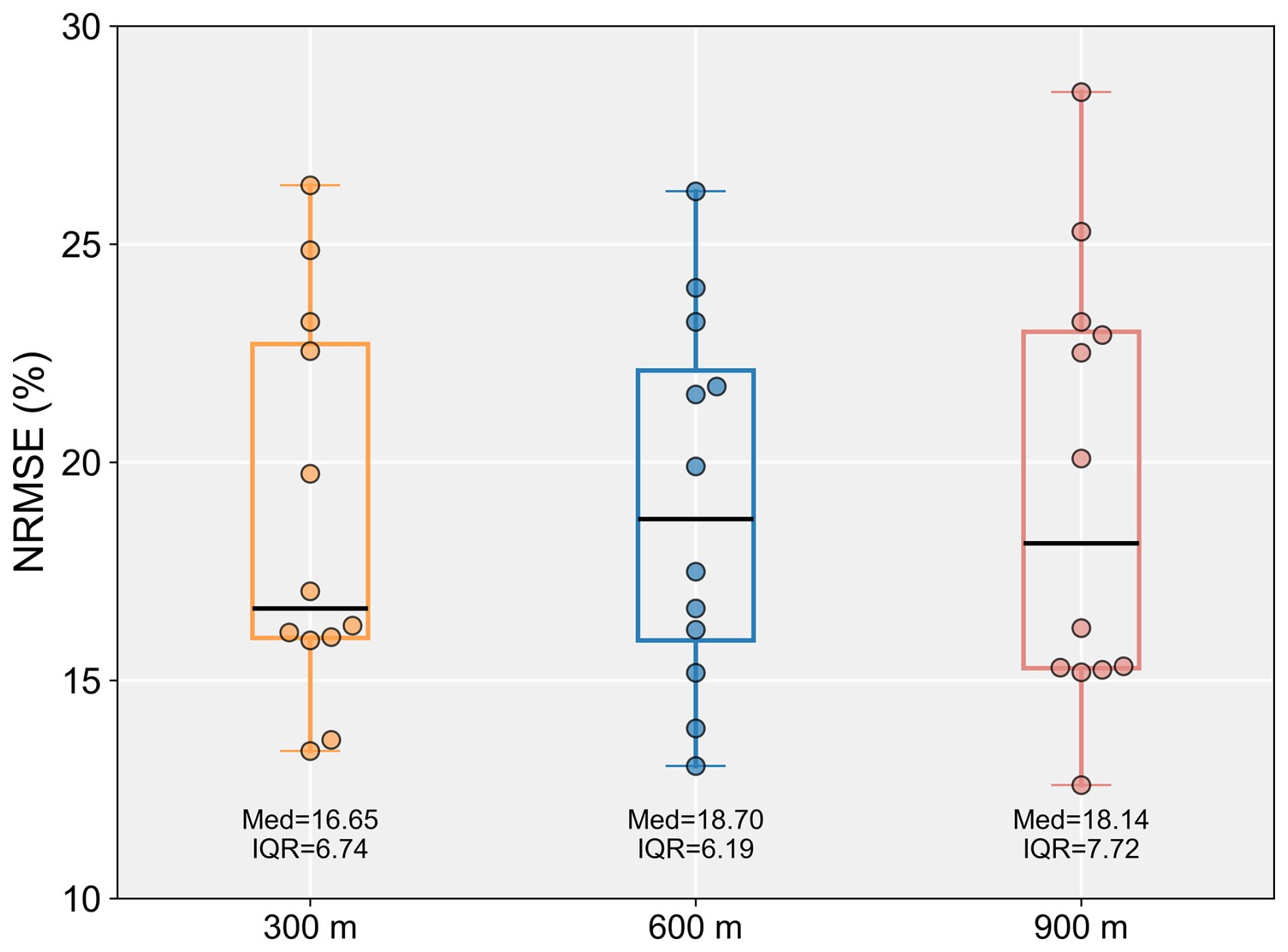
Figure 11 Box plots of NRMSE (%) for buffer distance sensitivity experiments (300, 600, and 900 m). Box ranges represent the upper and lower quartiles, and whiskers extend to 1.5 times the interquartile range.

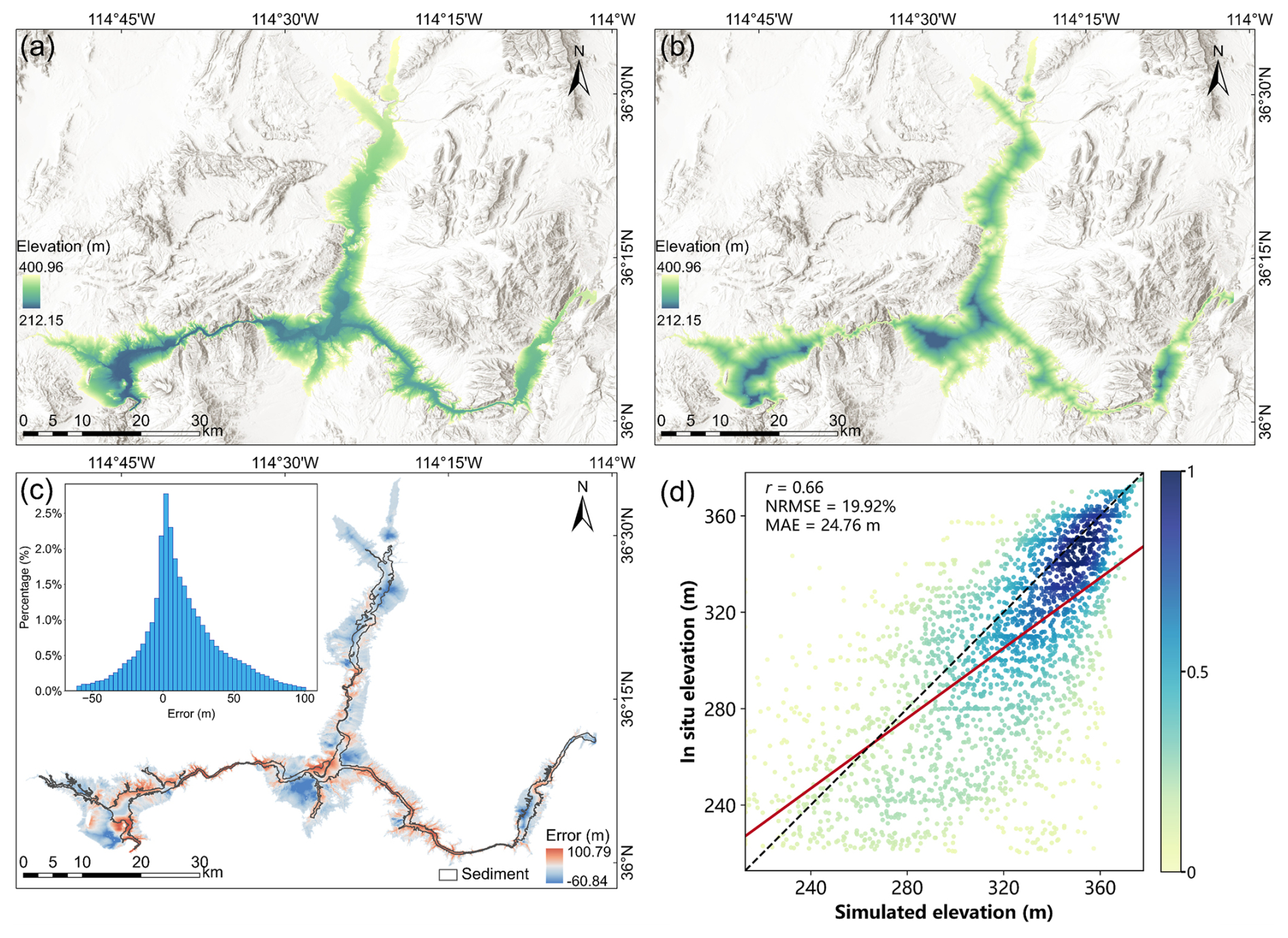
Figure 12 In situ and simulated bathymetric maps of Lake Mead, along with accuracy evaluation results. (a) In situ bathymetric map. (b) Simulated bathymetric map. (c) Error map between simulated and in situ results, accompanied by a histogram of error distribution. (d) Scatter plot comparing simulated and in situ bathymetric values.

We further assessed how bathymetric accuracy responds to the distance of the dynamic exposed area used to calculate shoreline slope by testing maximum buffer widths of 300, 600, and 900 m (Fig. 11). The median NRMSEs are similar across the three settings (16.65 %, 18.00 %, and 18.14 %, respectively), indicating that overall performance is not strongly sensitive to buffer width within the tested range. However, error dispersion increases with buffer size, with the 900 m setting exhibiting the largest interquartile range (IQR = 7.72) and a more pronounced upper tail. This suggests that overly wide buffers may incorporate broader-scale topographic signals unrelated to the representative nearshore slope (e.g., terraces or distant hillslopes), thereby degrading performance for some lakes. In contrast, the 600 m setting yields the smallest IQR (6.19) and the most consistent results across lakes; it is therefore adopted as the default in this study. Notably, because our workflow determines an adaptive buffer extent using the multi-level buffering scheme described in Sect. 2.2.1, the specified value represents the maximum buffer distance and is not necessarily reached for all lakes. In some cases, the optimal buffer is identified at a shorter distance, so the maximum value is not applied.

4.3 Method extension and applicability

To evaluate the applicability of the proposed method, we conducted a case study on Lake Mead in the United States (36.25° N, 114.39° W). As an artificial reservoir, Lake Mead differs significantly from the natural lakes analyzed in this study. Being a river-type reservoir, its underwater topography exhibits significant spatial heterogeneity across different sections of the river channel. Moreover, unlike many lakes on the Tibetan Plateau, which are characterized by thick sediment layers, sediment deposition in Lake Mead is primarily concentrated within the central river channel (Fig. 12c), resulting in a relatively flat underwater terrain (Rosen and Van Metre, 2010). To account for these characteristics, the sediment correction module was applied selectively – targeting only the central portion of the profile – during simulation. This tailored approach enabled the generation of a bathymetric map for Lake Mead (Fig. 12b) that more accurately reflects its distinct geomorphological features.

The simulated underwater elevation map (Fig. 12a) showed an overall consistent pattern and morphology with the in situ bathymetric map (Fig. 12b). The error distribution was predominantly centered around zero, although localized areas of noticeable overestimation and underestimation were evident (Fig. 12c). Overestimations primarily occurred in the sediment-rich areas, which correspond to the original pre-impoundment riverbed. In these regions, applying the correction formula from Eq. (6) led to an underestimation of the slope, thereby contributing to the overestimated elevations. To quantitatively assess the simulation accuracy, 2500 validation points were randomly selected across the entire lake, and the results were visualized in a scatter plot (Fig. 12d). The results revealed a strong correlation between in situ and simulated water depths (r=0.66). A significant concentration of validation points was observed at elevations above 300 m, while point dispersion amplified with decreasing elevation, indicating greater uncertainty at deeper sections of the lake. Overall, simulation performance tended to degrade with increasing depth. Despite these challenges, the results demonstrate that the proposed method has promising potential for application in lakes and reservoirs across diverse environmental conditions and geomorphological settings.

5 Conclusion

This study presents a cost-effective method for predicting underwater terrain and lake water storage using DEM data. The proposed approach integrates terrain continuity with lake level recession principles. Applied to 12 lakes on the Tibetan Plateau, the method demonstrates strong performance, achieving an average r of 0.72 and an APE of 23.47 % for lake water storage estimates. The simulated bathymetric maps effectively capture underwater terrain variations, providing an effective solution for reconstructing lake depth in areas lacking direct measurements. The primary source of uncertainty in the method stems from the vertical accuracy of the DEM data and error propagation during the simulation process. Since the DEM is the sole input, its quality significantly affects each simulation step. Although NASADEM has demonstrated relatively high vertical accuracy, topographic errors may still affect results, especially in large-scale applications. Furthermore, simulation errors tend to accumulate as the model progresses from the shoreline toward the lake center, explaining why depth estimates are generally more accurate near the shoreline than in the deeper central areas of the lake. Relatively large errors were primarily observed in lakes with shallow water depth, complex basin morphology, or strong local sedimentation effects, where the topographic continuity between the shoreline and the underwater terrain may be weaker. Under such conditions, the uncertainty of bathymetric reconstruction is more likely to increase.

To improve accuracy and address current limitations, future efforts should focus on integrating multi-source datasets. For example, incorporating satellite laser altimetry data (e.g., ICESat-2), which can partially penetrate water surfaces, could provide valuable constraints for underwater topography estimation. While satellite altimetry alone cannot fully capture underwater elevations, its integration could reduce systematic errors and mitigate the inherent shortcomings of DEM-based methods. Building on this foundation, future work will explore the use of radar and LiDAR elevation data to better represent submerged terrain and aim to develop an automated, adaptive framework for lake bathymetry estimation tailored to lake-specific characteristics. Additionally, efforts will be directed toward advancing higher-precision methods for generating lake depth maps, further enhancing the reliability of large-scale hydrological and ecological assessments.