Triple collocation validates CONUS-wide evapotranspiration inferred from atmospheric conditions

Large-scale estimation of evapotranspiration (ET) remains challenging because no direct remote sensing estimates of ET exist and because most data-driven estimation approaches require assumptions about the impact of moisture conditions and biogeography on ET. The surface flux equilibrium (SFE) approach offers an alternative, deriving ET directly from atmospheric temperature and humidity under the assumption that conditions in the atmospheric boundary layer reflect ET's land boundary condition. We present a 4 km resolution, continental United States-wide, daily ET dataset spanning from 1979 to 2025 using the SFE method. The Bowen ratio is first calculated using the SFE method solely based on temperature and specific humidity estimates from gridMET and then converted to ET using net radiation and ground heat fluxes from ERA5-Land. We evaluate its performance using extended triple collocation to estimate the standard deviation of the random error and the correlation coefficient of SFE ET compared to true ET, as well as those of three widely used alternative ET datasets: GLEAM, FluxCom, and ERA5-Land. Despite its extreme simplicity, SFE ET achieves performance comparable to or exceeding the other datasets across large portions of CONUS, particularly in the Western U.S., while requiring no information about land surface, vegetation, or soil properties and no assumptions about ET's response to environmental and climate drivers. Our results support the use of SFE as a scalable, observation-driven method for estimating ET.

1 Introduction

Evapotranspiration (ET) dominates the terrestrial water cycle (Friedlingstein et al., 2019; Good et al., 2015), controls the partitioning of radiation into latent and sensible heat (McColl and Rigden, 2020), and plays a key role in driving the hydrologic cycle by returning water to the atmosphere (Oki and Kanae, 2006). ET therefore has downstream feedbacks on temperature (Teuling et al., 2010), precipitation, and vegetation productivity (Green et al., 2017) in addition to directly impacting the carbon cycles through the trade-off between photosynthesis and transpiration (Yang et al., 2023). However, estimation of ET via remote sensing remains a significant challenge with implications for understanding of vegetation response to drought, fire risk, and the accounting of freshwater resources.

One challenge for ET remote sensing is that, unlike some surface properties such as temperature, we are unable to directly sense the flux of water or latent heat associated with ET electromagnetically. Therefore, ET products must leverage modelling approaches – either physical, hybrid, or machine learning – constrained by the data that is observable via remote sensing. These modelling approaches for ET often assume – implicitly or explicitly – the response of evaporation and transpiration to environmental drivers, such as drought or variations in land cover.

Alternatively, surface flux equilibrium (SFE) is a data-driven method for estimating ET directly from atmospheric conditions without relying on soil or vegetation parameterization. The concept of surface flux equilibrium was first proposed by McColl et al. (2019) and states that, under many circumstances, the atmosphere and land surface are coupled so that changes in surface fluxes (including ET) are reflected in atmospheric temperature and humidity. This approach has several advantages over other ET estimation methods. It requires no information about vegetation, soil, or subsurface properties. It also makes no assumptions about root-zone moisture status or vegetation response to water availability. This means it is well suited for hydrological research attempting to interrogate the relationship between ET and water availability or between ET and vegetation cover (or other biogeographic drivers). Additionally, SFE includes no tunable parameters and can be computed easily using only three inputs – air temperature, humidity, and net radiation – each of which is readily available at global scales (McColl and Rigden, 2020).

However, more complex ET estimation methods would be expected to outperform SFE in many settings due to its extreme simplicity and lack of adjustable parameters. Nevertheless, previous SFE implementation and validation efforts indicate that SFE performance is comparable – or even better than – other ET estimation methods at the point- and watershed- scale (Chen et al., 2021; McColl and Rigden, 2020; Thakur et al., 2025). For example, SFE ET has been found to be within the range of in situ measurement uncertainty at a selection of inland eddy covariance towers, an upper limit on the performance of any ET estimate (McColl and Rigden, 2020). Thakur et al. (2025) also calculated SFE ET at inland eddy covariance sites across the continental United States (CONUS) using tower-based temperature, humidity, and net radiation. They found that SFE ET outperformed remotely sensed ET from MODIS (Mu et al., 2011) as well as from three ET algorithms using data from the ECOsystem Spaceborne Thermal Radiometer Experiment on Space Station (ECOSTRESS): the Simplified Surface Energy Balance (Savoca et al., 2013) SSEBop, (Savoca et al., 2013), the atmosphere-land exchange inverse disaggregation algorithm (DisALEXI) and the Priestley-Taylor Jet Propulsion Laboratory model (PT-JPL, Fisher et al., 2020).

Thakur et al. (2025) further investigated the impact of input data on SFE performance by calculating SFE ET using three scenarios: only eddy covariance data, by using the North American Land Data Assimilation System (NLDAS, Xia et al., 2012) for temperature and humidity and the Clouds and the Earth's Radiant Energy System instrument (CERES, Doelling et al., 2013) for net radiation, and by finally using NLDAS for temperature and humidity and MODIS for net radiation. All three SFE ET implementations compared favorably to tower-based ET with R² of 0.70, 0.68, and 0.67 for the tower-based SFE, CERES-based SFE, and MODIS-based SFE, respectively. This suggests that the emergent simplicity of ET that SFE takes advantage of is robust to choices of input data, at least at the scale of eddy covariance towers.

The only gridded estimates of SFE ET are reported by Chen et al. (2021), who calculated monthly ET at 0.125° across CONUS using net radiation from CERES and 2 m temperature and humidity from North American Regional Reanalysis (NARR, Mesinger et al., 2006). They compared SFE ET to estimates from the Coupled Model Intercomparison Project phase 6 (CMIP6, Eyring et al., 2016) and to water balance-based ET estimates available at large catchments across CONUS. The error in the water balance-based estimates provides a minimum possible error, below which ET estimation approaches cannot be distinguished due to errors in the underlying reference data. They found that SFE ET errors are comparable to the error of the catchment water balances and that SFE outperforms the reanalysis (NARR) and most CMIP6 91 models.

However, even this sole gridded implementation of SFE – while promising – is unable to provide a thorough evaluation of the SFE approach because the comparison datasets each have their own unquantified uncertainties. Therefore, disagreement between SFE and CMIP6 cannot be attributed to either dataset because their errors cannot be distinguished. One solution to this is the statistical evaluation approach of triple collocation. Using triple collocation and its 7 updated counterpart, extended triple collocation (McColl et al., 2014), it is possible to compare three datasets with co-located measurements and estimate two important performance metrics: (1) the variability in the random error of each dataset and (2) the correlation between the measured value and the underlying “true” variable. Both performance metrics can be calculated without reference to this unknowable “true” variable, in this case ET, and without assuming the error of any of the three comparison datasets.

Triple collocation – sometimes also referred to as the “three-cornered hat” approach – has been widely used in evaluating datasets where a “truth” or reference dataset is unavailable, for example in the evaluation of datasets for soil moisture (Draper et al., 2013; Gruber et al., 2016; Scipal et al., 2008), ocean winds (Caires and Sterl, 2003), precipitation (Alemohammad et al., 2015, Burnett et al., 2020), sensible heat and carbon fluxes (Alemohammad et al., 2017), ET (Khan et al., 2018), near-surface air temperature and specific humidity (Sun et al., 2021), and terrestrial water storage (Ferreira et al., 2016). It can also be used to estimate the coupling of multiple variables, for example latent heat and soil moisture (Crow et al., 2015). Given three datasets with observations of the same state variable, each with their own non-correlated random errors, comparison of the three datasets via triple collocation enables calculation of each dataset's random error variance (Stoffelen, 1998).

Here, we accomplish two steps in advancing the estimation of ET. First, we release the first publicly available, gridded dataset of daily SFE ET. We calculate this dataset at 4 km resolution across the continental United States (CONUS) using gridMET for 2 m temperature and humidity and net radiation from ERA5-Land. Second, we compare our gridded estimates of SFE ET to three other remotely sensed ET estimates: Global Land Evaporation Amsterdam Model Version 4 (GLEAM, Miralles et al., 2011), FluxCom (Jung et al., 2019), and ERA5-Land (Muñoz-Sabater et al., 2021). In addition to comparing the spatial pattern and variance of all datasets, we further use the statistical method of extended triple collocation following McColl et al. (2014) to calculate the error statistics of each dataset, despite lacking observations of “true” ET (Gruber et al., 2016; McColl et al., 2014; Stoffelen, 1998).

2 Methods

2.1 Calculating ET from atmospheric conditions assuming surface flux equilibrium

We calculate daily ET after McColl et al. (2019) by assuming that the near-surface atmosphere is in a state of “surface flux equilibrium” where atmospheric conditions at the boundary layer reflect the recent fluxes of latent (λE) and sensible (H) heat on the Earth's surface. If this is the case, then increasing ET (i.e. increasing latent heat) will correspond with diminished sensible heat and result in both atmospheric cooling and increased humidity. The ratio of sensible and latent heat fluxes – known as the Bowen ratio (B) – can therefore be approximated by temperature and humidity at the boundary layer, so long as atmospheric conditions reflect the integrated signal of fluxes on the Earth's surface.

We use 2 m air temperature (T_a) and relative humidity (q_a) from gridMET (Abatzoglou, 2013) to estimate the Bowen ratio, where R_v=461.5 (J kg⁻¹ K⁻¹) is the gas constant for water vapor, C_p=1005 (J kg⁻¹ K⁻¹) is the specific heat capacity of air at constant pressure, and λ=2.56 139 × 106 (J kg⁻¹) is the latent heat of vaporization of water (Eq. 1).

$$\begin{array}{}\text{(1)}& B={\displaystyle \frac{H}{LE}}\approx {\displaystyle \frac{R_{\mathrm{v}}{c}_p{T}_{\mathrm{a}}^{\mathrm{2}}}{{\mathit{\lambda }}^{\mathrm{2}}{q}_{\mathrm{a}}}}\end{array}$$

We choose gridMET because it downscales output from the North American Land Data Assimilation System (NLDAS) with PRISM. This incorporation of statistically interpolated station data at a fine resolution helps gridMET achieve a high correlation with in situ stations, particularly for the variable of temperature, while maintaining a relatively fine spatial resolution of 4 km across CONUS (Abatzoglou, 2013). Net radiation (R_n) allows conversion from the Bowen ratio to ET (Eq. 2). We use R_n from ERA5-Land (Muñoz-Sabater et al., 2021) because of its high agreement with in situ measurements across CONUS (Yin et al., 2023). However, we note that error in these input datasets will propagate to error in the resulting ET estimates.

Although the ground heat flux (G) can vary from 10 % to as much as 50 % of R_n depending on ground cover (Clothier et al., 1986, Santanello and Friedl, 2003), here we assume a constant G of 10 %. Additionally, we do not evaluate SFE ET on any days with negative R_n because doing so would result in a negative ET estimate, which is not physical.

$$\begin{array}{}\text{(2)}& \mathit{\lambda }\mathrm{ET}=(\mathrm{1}+B{)}^{-\mathrm{1}}(R_{\mathrm{n}}-G)\end{array}$$

2.2 Triple collocation error estimation

Triple collocation assumes a linear error model for each dataset, where the observed value for a given dataset (x) is assumed to be a linear function of the “true” ET (T) obscured by a constant additive bias (α), a constant multiplicative bias (β) and a time-varying additive random error with zero mean (ϵ) (Eq. 3). While a linear error model likely does not fully capture the error structure of the actual ET dataset errors, it has been successfully used to evaluate ET datasets using triple collocation in other regions (Kahn et al., 2018; He et al., 2023).

$$\begin{array}{}\text{(3)}& x_i={\mathit{\alpha }}_i+{\mathit{\beta }}_{i}T+{\mathit{ϵ}}_i\end{array}$$

In addition to assuming a linear error model for each dataset, triple collocation further assumes that the errors of each dataset are stationary and uncorrelated both with each other and with the unknown truth (Gruber et al., 2016; McColl et al., 2014).

With these assumptions, the variance of each dataset (Q₁₁, Q₂₂, and Q₃₃) represents the sensitivity of the dataset to variations in the true signal (via the product of β_i and σ_T) plus the variance of the random error (${\mathit{\sigma }}_{\mathit{ϵ}i}^{\mathrm{2}}$) (Eq. 4).

$$\begin{array}{}\text{(4)}& Q_{ii}={\mathit{\sigma }}_i^{\mathrm{2}}={\mathit{\beta }}_i^{\mathrm{2}}{\mathit{\sigma }}_T^{\mathrm{2}}+{\mathit{\sigma }}_{\mathit{ϵ}i}^{\mathrm{2}}\end{array}$$

Covariance between pairs of datasets (e.g. Q₁₂, Q₁₃, and Q₂₃) likewise provides information about each dataset's sensitivity to the true unknown ET via β_i and σ_T. (Eq. 5).

$$\begin{array}{}\text{(5)}& Q_{ij}={\mathit{\sigma }}_{ij}^{\mathrm{2}}={\mathit{\beta }}_i{\mathit{\beta }}_j{\mathit{\sigma }}_T^{\mathrm{2}}\end{array}$$

The β_i and σ_T terms cancel out for the ratio of each dataset covariance pair, resulting in six equations and six unknowns. These can be solved to calculate the standard deviation of the random error of each dataset, σ_ε (Eq. 6).

$$\begin{array}{}\text{(6)}& {\mathit{\sigma }}_{\mathit{\epsilon }}=\left[\begin{array}{l}\sqrt{Q_{\mathrm{11}}-\frac{Q_{\mathrm{12}}{Q}_{\mathrm{13}}}{Q_{\mathrm{23}}}}\\ \sqrt{Q_{\mathrm{22}}-\frac{Q_{\mathrm{12}}{Q}_{\mathrm{23}}}{Q_{\mathrm{13}}}}\\ \sqrt{Q_{\mathrm{33}}-\frac{Q_{\mathrm{13}}{Q}_{\mathrm{23}}}{Q_{\mathrm{12}}}}\end{array}\right]\end{array}$$

The absolute values of β_i cannot be separated from the absolute value of σ_T. However, many studies assume β_i=1 for one dataset – effectively choosing it as a reference dataset which has no multiplicative bias – and calculate β_i for the other two datasets relative to the actual unknown multiplicative bias of the reference dataset. In this study, however, we do not separate β_i and σ_T.

Extended triple collocation further allows the calculation of the correlation between each dataset and the unknown truth, R_T, while requiring no additional information (McColl et al., 2014); Eq. 7).

$$\begin{array}{}\text{(7)}& R_T^{\mathrm{2}}=\left[\begin{array}{l}\frac{Q_{\mathrm{12}}{Q}_{\mathrm{13}}}{Q_{\mathrm{11}}{Q}_{\mathrm{23}}}\\ \\ \frac{Q_{\mathrm{12}}{Q}_{\mathrm{23}}}{Q_{\mathrm{22}}{Q}_{\mathrm{13}}}\\ \\ \frac{Q_{\mathrm{13}}{Q}_{\mathrm{23}}}{Q_{\mathrm{33}}{Q}_{\mathrm{12}}}\end{array}\right]\end{array}$$

Triple collocation requires several assumptions, all of which are likely to be at least partially violated (e.g., Yilmaz and Crow, 2014). However, these assumptions are not unique to triple collocation. Gruber et al. (2016) showed that more common validation strategies implicitly require the same assumptions. For example, if we were to instead estimate the correlation coefficient and root-mean-squared error (RMSE) between SFE ET and another reference ET product, we would be implicitly making the same assumptions.

2.3 Comparison ET datasets

We compare SFE ET to ET from FluxCom, GLEAM version 4, and ERA5-Land. We compare all ET datasets over the years 1980 to 2016, which represents the maximum overlap in temporal coverage between all four datasets. Additionally, we resample each dataset to match the native resolution of FluxCom at 0.5°. We match the FluxCom resolution because it is the coarsest. We choose to compare SFE to these particular three ET datasets not just because they are commonly used, but also to minimize violation of the triple collocation assumptions, particularly the assumption of independent errors between datasets. This is commonly achieved by using datasets that differ in their input data sources and modeling frameworks (Gruber et al., 2016; McColl et al., 2014). We also remove the seasonal cycle from each dataset by subtracting the 30 d rolling average from each day (Chen et al., 2018; Draper et al., 2013; Miralles et al., 2010). This ensures that differences in the seasonality and timing of ET do not impact the triple collocation analysis and has been shown to improve error estimation with triple collocation for ET datasets specifically (He et al., 2023). Performing triple collocation on the anomaly should also reduce violation of the assumption that the ET error structure is linear. This is because the low-frequency (e.g. seasonal) ET signals which are removed are expected to have a different non-linearity than the high-frequency signals isolated by the anomaly (Miralles et al., 2010; Su et al., 2014).

After removing the seasonal cycle, we choose only the months of March through October for the triple collocation analysis. This is because negative daily net radiation occurs for some pixels during the winter months, prohibiting the calculation for SFE. Because the number of days with negative net radiation varies for each pixel, we eliminate all winter months for all datasets to ensure a consistent number of data for each dataset and pixel.

Finally, we use extended triple collocation to calculate the standard deviation of the random error and the correlation coefficient of each dataset (see Sect. 2.2 above). Because we have four comparison datasets and triple collocation requires just three, we are able to repeat our estimates of each dataset's error statistics once for each possible “triplet” (i.e. combination) of three datasets. Convergence of the error estimates regardless of the triplet chosen increases our confidence in the robustness of the triple collocation assumptions and therefore in our calculated values (Draper et al., 2013; He et al., 2023). In addition to performing triple collocation, we also compare the four datasets via a general analysis of the variance and spatial patterns of ET.

The FluxCom dataset we choose for our triple collocation analysis uses machine learning to upscale eddy covariance measurements from flux towers based on satellite and meteorological inputs. FluxCom provides an ensemble of latent heat estimates trained using different meteorological datasets. In order to have the longest data record with daily resolution, here we use the single FluxCom ensemble member trained with the CRUNCEPv6 reanalysis product (Wei et al., 2014), as opposed to the mean of all possible FluxCom ensemble members. However, the different model setups (each with a different weather model) were previously found to have similar performance (Jung et al., 2019). In addition to the climate data from CRUNCEP, FluxCom uses radiation data from CERES (Doelling et al., 2013), precipitation from the Global Precipitation Climatology Project (GPCP, Huffman et al., 2001), and temperature, land cover, and other reflectance indicators from MODIS. The FluxCom model is run per plant functional type and then combined into a single estimate by weighting each plant functional type's fractional areal coverage of the pixel (Jung et al., 2019).

GLEAM estimates ET by using remote sensing and reanalysis data to force a hybrid model which includes modules for canopy interception, potential evapotranspiration, soil water content, and vegetation response to evaporative stress. Although FluxCom and GLEAM have some remote sensing inputs in common, for example radiation from CERES and vegetation information from MODIS, Gleam Version 4 takes a hybrid modelling approach and does not rely fully on machine learning like FluxCom. Specifically, GLEAM version 4 primarily uses physical modelling modules with only a single module – for evaporative stress – using a deep neural network trained using in situ data from eddy covariance towers and sap flow measurements (Koppa et al., 2022; Martens et al., 2017; Miralles et al., 2025). This is in contrast to GLEAM version 3, which estimates evaporative stress empirically as a function of soil moisture and vegetation optical depth – both from microwave remote sensing inputs. Additionally, GLEAM Version 4 calculates ET using Penman's equation (as opposed to Priestley-Taylor, used in Version 3) and also updates the multi-layer water balance model so that vegetation access to groundwater can be represented. However, in GLEAM Version 4, plant rooting depths are static for each land cover within the groundwater scheme and there is still a prescribed multiplicative stress function to determine how vegetation responds to soil moisture stress. GLEAM is the only dataset in our comparison set which partitions ET between evaporation, transpiration, and interception. We use the variable referring to the total evaporation (E) to best match the other ET estimates.

Finally, ERA5-Land uses the near-surface atmospheric reanalysis from ERA5, which assimilates observations from a range of satellites and in situ observation networks for many variables including land surface temperature, precipitation, wind speed, and soil moisture (Hersbach et al., 2020). ERA5-Land then takes the atmospheric states from ERA5 and re-runs the land surface model component at a finer resolution (9 km) offline (Muñoz-Sabater et al., 2021). This allows for additional and refined land surface parameterizations and corrections. Unlike FluxCom and GLEAM, ERA5-Land has no machine learning components. For our analysis, we sum the hourly latent heat flux output of ERA5-Land to daily totals and then resample bilinearly to match the coarser 0.5° FluxCom grid. Finally, both ERA5-Land and FluxCom report latent heat flux in units of energy per unit area, which we convert to ET (mm d⁻¹) by dividing by the latent heat of vaporization ($\mathit{\lambda }=\mathrm{2.56}\times \mathrm{106}$ J kg⁻¹).

2.4 Comparing performance across biogeographical factors

We compare the resulting σ_ε and R_T estimates from triple collocation across a variety of biogeographical factors – specifically climate, elevation, land cover type, and the distance to the coast – to better understand under what conditions SFE ET performs well and how its performance across biogeography compares to that of the other ET estimates.

We calculate the mean annual precipitation at each pixel using monthly precipitation (P) from 1991 to 2020 from TerraClimate (Abatzoglou, 2013).We use elevation from MERIT Hydro (Version 1.0.1., Yamazaki et al., 2019). For land cover, we use the National Land Cover Database (NLCD) land cover map from 2021 (Dewitz, 2024). We consider the land cover types of forest (combining deciduous, evergreen, and mixed forests), shrub, grassland, wetland (combining woody and herbaceous wetlands), and agricultural (cultivated crops).

We further analyze the performance of each dataset by each pixel's distance from the coast because the assumptions of SFE are likely to be violated near the ocean (McColl et al., 2019). This is because in coastal regions, ocean moisture and temperature are expected to be a strong control on land surface fluxes. We calculate the distance of each pixel centroid from the nearest coast using the TIGER/Line Coastline National Shapefile (United States Census Bureau, 2019). We also exclude pixels from all analyses if their centroid overlaps with the ten largest water bodies in CONUS (ArcGIS Data and Maps, 2023).

3 Results

3.1 Surface flux equilibrium ET across CONUS from 1979 to 2025

Here, we publicly release a dataset of daily SFE ET from 1979 to 2025 at 4 km resolution across CONUS (see Data Availability section). The spatial mean (shown in Fig. 1a) follows expected patterns across CONUS – with an aridity driven gradient from West to East and a radiation driven gradient from North to South in the Eastern US. This spatial pattern exists regardless of the choice of parameter for the ground heat flux (G), although the magnitude of mean annual ET is altered (Fig. S1). The temporal variability in daily ET calculated using the SFE approach is consistent with the comparison datasets (Fig. S2). However, SFE has a larger standard deviation across much of CONUS – particularly the Western US – than FluxCom and GLEAM. Across several sample pixels, chosen as heavily vegetated examples spanning multiple regions, the seasonal cycle of mean annual ET is likewise comparable across all four ET estimates, although the timing of maximum summer ET each year varies between datasets (Fig. 1b–g).

The magnitude of mean annual continental SFE ET (Fig. 2) and the pattern of interannual variability which matches SFE the best is that of GLEAM (ρ=0.55). The two datasets with the overall closest match in ET interannual variability, however, are FluxCom and ERA5-Land (ρ=0.71). All correlation coefficients are shown in Table S1. Although SFE and FluxCom each have intermediate magnitudes of mean continental ET relative to GLEAM and ERA5, both datasets – and FluxCom in particular – also have the lowest interannual variability magnitude (8 mm yr⁻¹ standard deviation for FluxCom and 10.5 mm yr⁻¹ for SFE, compared to 22 and 28 mm yr⁻¹ for ERA5-Land and GLEAM, respectively). Across the entire average record, the mean annual ET from SFE (538 mm yr⁻¹) is just below GLEAM (552 mm yr⁻¹), with ERA5-Land having the highest mean annual ET (645 mm yr⁻¹). The mean annual ET across CONUS is shown in Table S2.

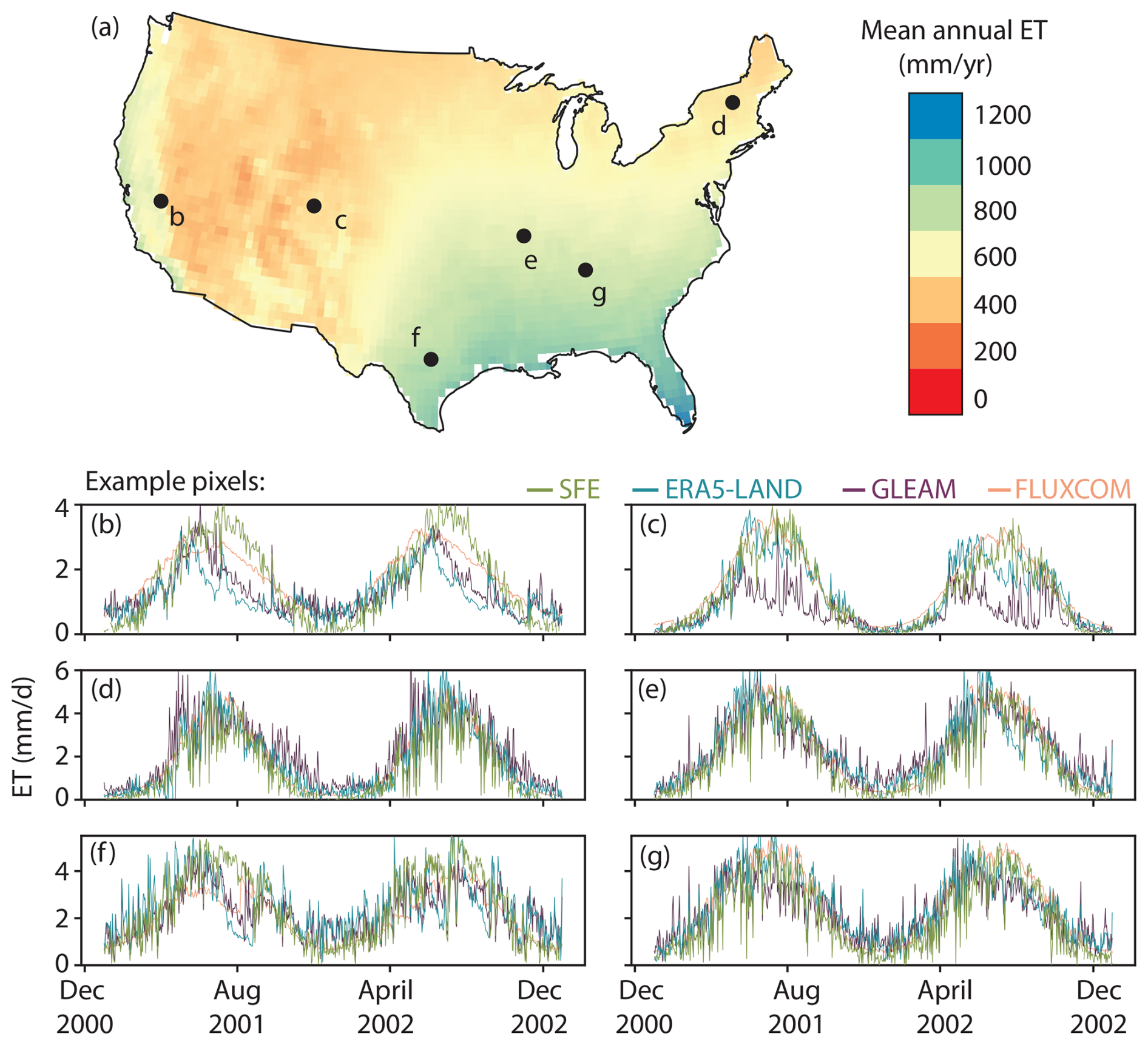
Figure 1 Mean annual SFE ET across CONUS from 1979 to 2025. Points show timeseries for example pixels for SFE (green), ERA5-Land (blue), GLEAM (purple) and FluxCom (pink).

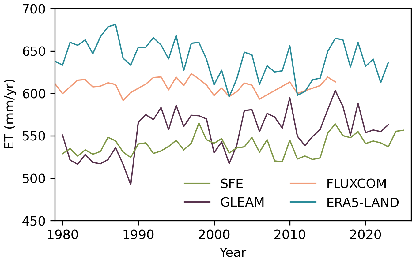
Figure 2 Interannual variability in mean annual ET across CONUS from 1979 through the record length of each dataset.

3.2 SFE is the only dataset that performs well in terms of both the standard deviation of the random error and the correlation coefficient

SFE performance during non-winter months as estimated by triple collocation is comparable – and even exceeds – the performance of the comparison datasets across much of CONUS, despite its extreme simplicity, lack of tunable parameters, and relatively small number of assumptions (Fig. 3). SFE, FluxCom, and GLEAM show a strong divide in performance between the Western and Eastern US. SFE and FluxCom both have the lowest σ_ε and highest R_T in the Western US compared to the Eastern US. In contrast, GLEAM has lower σε in the Western US, but higher R_T in the Eastern US. ERA5-Land shows more heterogeneity in performance across space – especially compared to SFE and FluxCom – and has no clear performance gradient between the Western and Eastern US.

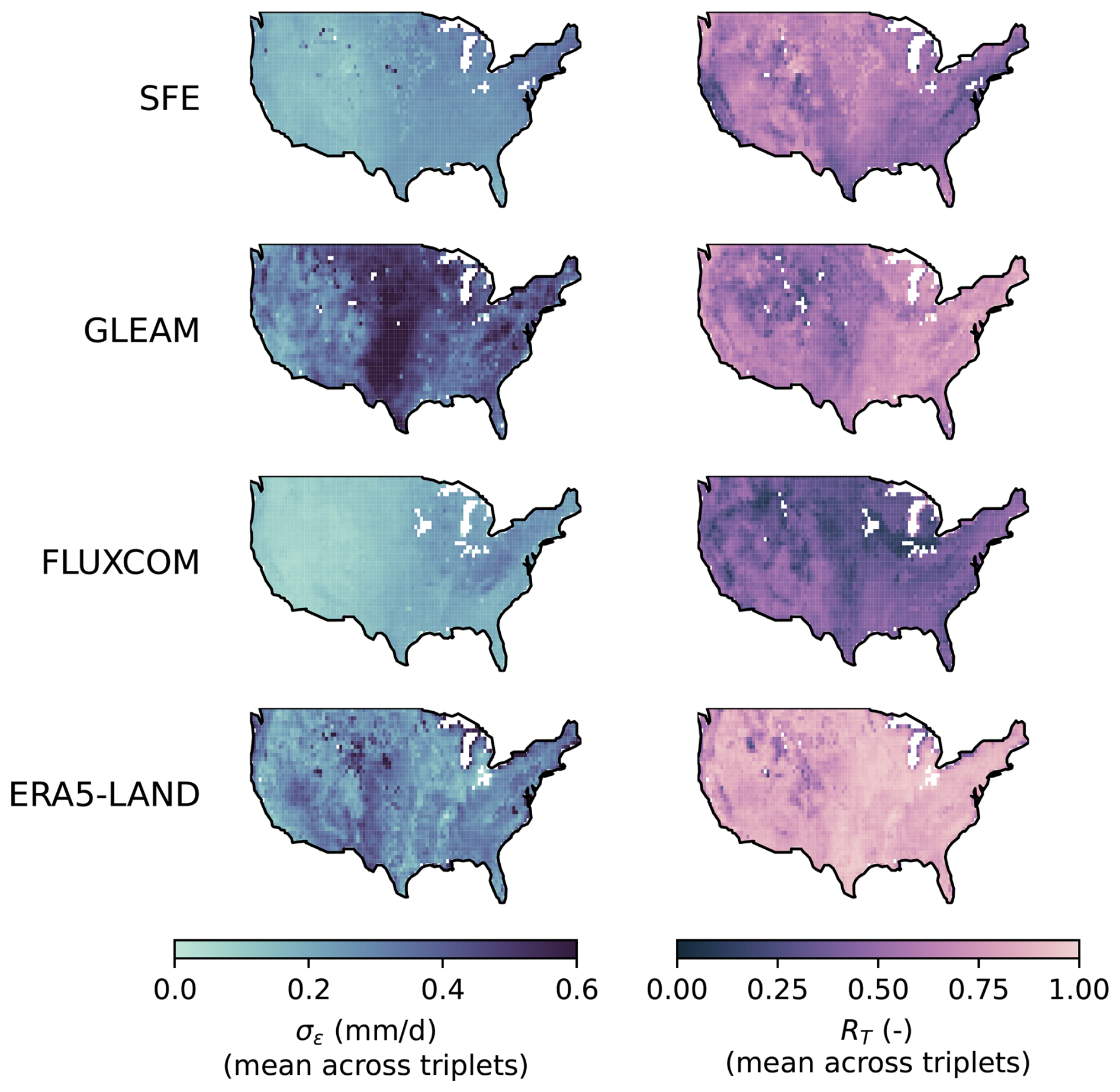
Figure 3 The standard deviation of the random error, σ_ε (left) and correlation coefficient to the truth, R_T (right) for each dataset averaged across all triplet combinations. Increasingly light colors are better performance. White pixels have no valid data for any triplet.

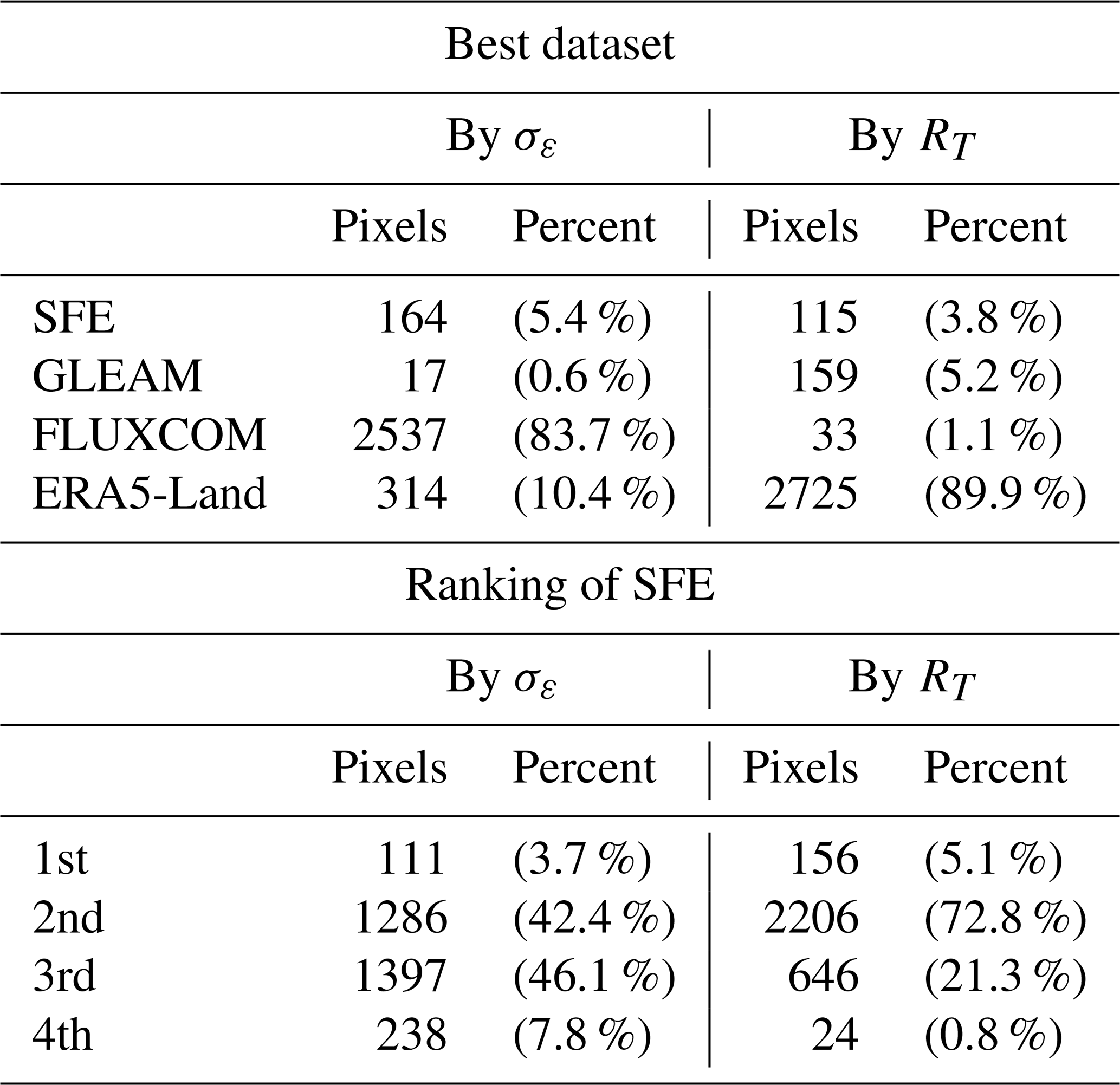
Despite its simplicity, SFE is the best or second-best dataset according to both σ_ε and R_T across more than half of CONUS (Fig. 4). SFE has the lowest or second lowest σ_ε and highest or second highest R_T across 46.1 % and 77.9 % of pixels across CONUS, respectively (Fig. 4, Table 1), mostly in the Western US.

SFE's high performance with regards to both σ_ε and R_T is unique among the comparison datasets. Other than SFE, the datasets with the best σ_ε and R_T, respectively, have the lowest performance for the complementary metric. For example, FluxCom has the lowest σ_ε across the majority of CONUS, but it also has the lowest R_T (Fig. 4). The opposite is true for ERA5, which is the highest performing dataset according to R_T across much of CONUS but frequently has the worst performance according to σ_ε, particularly in the US Southwest. SFE is the only dataset which consistently has high performance according to both metrics.

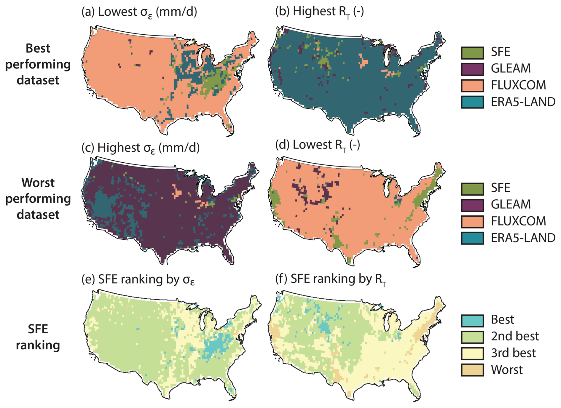
Figure 4 Summary of relative performance of all four datasets. The dataset with highest performance for the standard deviation of the random error, σ_ε (a) and the correlation coefficient with “true” ET, R_T (b) for each pixel. The worst performing datasets for σ_ε (c) and R_T (d). The relative ranking of SFE for σ_ε (e) and R_T (f). The total number of pixels (and relative percent of pixels) of each color are shown in Table S1. Pixels with centroids within 4 km of the border have been removed.

Table 1 (Top) The number of pixels where each dataset has the best performance according to the standard deviation of the random error, σ_ε, and the correlation coefficient to the truth, R_T. (Bottom) The number of pixels by SFE ET ranking.

We note that the estimates of σ_ε and R_T are consistent between triplets, indicating σ_ε and R_T estimates are robust to the choice of comparison datasets (Fig. 5). Individual σ_ε and R_T maps for each dataset and triplet combination are shown in Figs. S3 and S4 and differences between each triplet combination are shown in Figs. S5 and S6. However, not all pixels have valid results for each triplet combination, which occurs when either σ_ε is negative for one or more of the datasets or if any R_T are greater than one. Figure 6 shows the total number of triplets which are valid for each pixel. The triplets with the most invalid pixels are those where FluxCom and ERA5-Land are both included. Invalid pixels are also more common in the Eastern US rather than the Western US. Even in the East, however, SFE – our main estimate of interest – still has at least one valid triplet in 96 % of pixels and at least two valid triplets in 88 % of pixels. SFE has three valid triplets – the maximum possible number for our four dataset analysis – in 56 % of pixels. The triple collocation results are also relatively insensitive to the choice of the ground heat flux (G) parameter used in the calculation of SFE, although increases in G necessarily reduce ET estimates, and therefore also reduce σ_ε (Fig. S7). To the extent that uncertainty in G causes errors in the SFE ET estimate, it will also cause errors in estimates from other ET products, which must make similar assumptions or approximations for G.

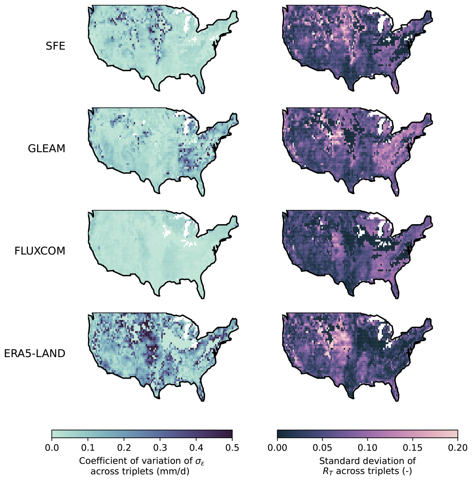
Figure 5 (left) The coefficient of variation of σ_ε for each dataset across all possible triplet combinations with valid data. White pixels have no valid data for any triplet. (right) The standard deviation of R_T for each dataset across all possible triplet combinations with valid data. White pixels have no valid data for any triplet and black pixels have only one triplet combination with valid data.

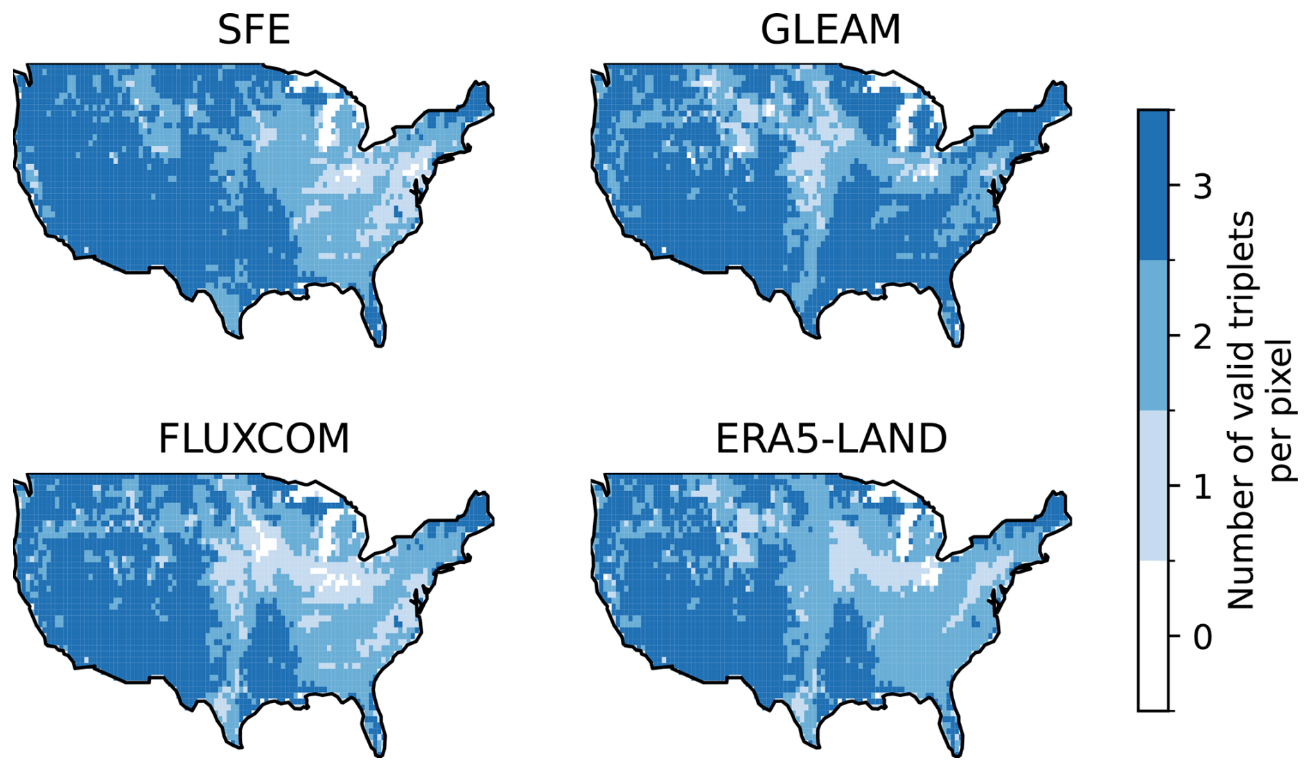
Figure 6 The total number of triple collocation estimates – one from each possible combination of datasets – that are averaged for each pixel and dataset combination. Pixels with no valid triple collocation results for any triplet are shown in white. The maximum number of valid triplets is three.

3.3 Performance across biogeographical factors

Comparing the trends of σ_ε (Fig. 7) and R_T (Fig. 8) across mean annual precipitation, elevation, landcover, and the distance to large water bodies shows that SFE performance is not more sensitive to any of these biogeographical factors than the comparison datasets. Even when comparing SFE performance with coastal proximity – a factor where we expect to see performance degradation due to the violation of SFE assumptions (McColl and Rigden, 2020) – the coastal proximity penalty of SFE is comparable to that of ERA5-Land. Indeed, ERA5-Land shows the sharpest decrease in performance within 20 km of the coast out of any of the datasets, however both SFE and ERA5-Land continue to show improved performance even up to 120 km inland. Neither GLEAM nor FluxCom have a strong relationship between coastal proximity and performance.

Likely due to its correlation with coastal proximity, SFE also has decreased performance at lower elevations with respect to both evaluation metrics. FluxCom and GLEAM likewise show their highest σ_ε at low elevations relative to higher elevations, with FluxCom σ_ε peaking around 500 m a.s.l. and GLEAM σ_ε around 1000 m a.s.l. All three datasets continue to have decreased σε as elevation increases. The relationship between elevation and R_T is relatively flat for SFE and FluxCom in the intermediate elevations, with the lowest R_T at the extreme low and high elevations. GLEAM and ERA5, however, have continuously decreasing R_T with increasing elevation, and the lowest R_T at elevations exceeding 2000 m a.s.l.

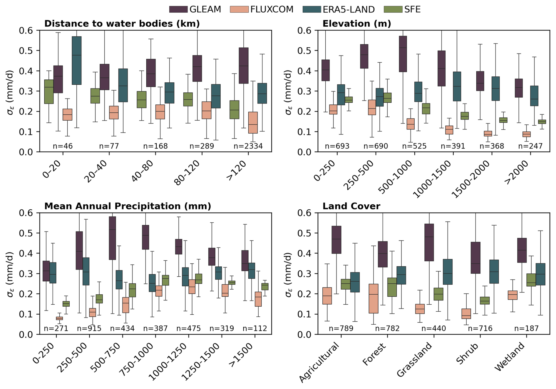
Figure 7 The standard deviation of the random error, σ_ε, for each ET dataset across mean annual precipitation, the distance to large water bodies, elevation, and land cover. The number of pixels in each category per ET dataset is shown below boxes.

The σ_ε for SFE, GLEAM, and FluxCom is lowest at the driest and wettest pixels and highest at pixels with intermediate precipitation. However, the σ_ε for GLEAM peaks at the 500–750 mm yr⁻¹ bin whereas FluxCom and SFE have the highest σ_ε at slightly wetter locations, receiving between 1000–1250 mm yr⁻¹. ERA5-Land, on the other hand, has a weaker relationship between mean annual precipitation and σ_ε. ERA5-Land has the opposite pattern than the other datasets and shows the highest σ_ε at the driest and wettest pixels with lower σ_ε at intermediate aridity. The relationship between mean annual precipitation and R_T follows that of mean annual precipitation and σ_ε in general, however R_T does not increase at the wettest pixels to the same degree as for the σ_ε. For example, SFE has continually decreasing R_T as mean annual precipitation increases with only a minimal increase in performance at the pixels with >1500 mm yr⁻¹ of precipitation.

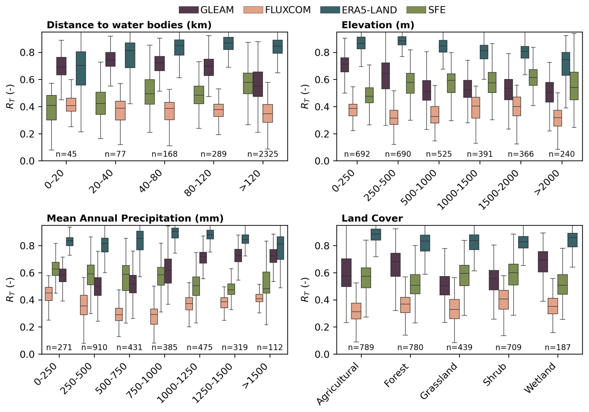
Figure 8 The correlation coefficient, R_T, for each ET dataset across mean annual precipitation, the distance to large water bodies, elevation, and land cover. The number of pixels in each category per ET dataset is shown below boxes.

The performance variability across land cover is not consistent between any of the datasets. ERA5-Land has the lowest σε and highest R_T in agricultural pixels, GLEAM in forest pixels, and FluxCom in shrubland pixels. The SFE R_T is similar across all land cover types but SFE σ_ε is highest in wetlands, followed by forest and agricultural pixels. Forested pixels also have a greater spread in σ_ε for FluxCom and SFE compared to the other land cover types. SFE σ_ε is lowest in shrublands, followed by grasslands. FluxCom σ_ε is likewise lowest for grassland and shrublands, which is the opposite of ERA5-Land, with the highest σ_ε in grasslands and shrublands.

4 Discussion

4.1 Which ET estimate is most accurate?

While triple collocation reveals that SFE is rarely the highest performing dataset for the non-winter months evaluated here, it is the second-best performing dataset across much of CONUS for both σ_ε and R_T (Fig. 4e, f). In addition, we find that datasets which outperform SFE only exhibit better performance for one – not both – of either σ_ε and R_T. That SFE performs well – although not the best – for both metrics suggests its usefulness for a variety of applications, particularly those where it is not clear a priori whether having high R_T or low σ_ε is most useful. Furthermore, SFE may be a particularly good choice for studies interested in the response of ET to water limitations. Unlike the explicitly assumed dependence of ET on hydrologic conditions in ERA5-Land or the implicitly assumed dependence of GLEAM and FluxCom (which is limited by the constraints of the machine learning structure and input data), SFE contains no a priori assumptions about the effect of water stress on ET, aside from any impact of these assumptions embedded in the interpolated temperature or humidity data used as an input to SFE calculation (such as for the gridMET data used here). Our release, alongside this manuscript, of a daily, 4 km resolution CONUS-wide dataset of SFE-based ET spanning 1979 to 2025 should facilitate future applications of SFE for scientific analyses. Additionally, there is no reason to believe that SFE should not perform similarly at the global scale, particularly outside of regions with substantial influence from ocean dynamics.

SFE is generally the second-best dataset regardless of metric, while alternative datasets with low random noise also have low correlation with the truth and vice versa. For example, across the four datasets tested, FluxCom has the lowest (most desirable) σ_ε across the majority of CONUS pixels (Fig. 4a). However, it also has the lowest (least desirable) R_T more often than any other datasets (Fig. 4d). ERA5-Land shows the converse relationship, with the highest (most desirable) R_T in almost all pixels compared to all other datasets, but poorer relative performance with regard to σε (Fig. 4b, c). How is this possible? To understand why, note that the triple collocation error model implies that,

$$\begin{array}{}\text{(8)}& R_{T,i}^{\mathrm{2}}={\displaystyle \frac{{\mathit{\beta }}_i^{\mathrm{2}}{\mathit{\sigma }}_T^{\mathrm{2}}}{{\mathit{\beta }}_i^{\mathrm{2}}{\mathit{\sigma }}_T^{\mathrm{2}}+{\mathit{\sigma }}_{\mathit{ϵ},i}^{\mathrm{2}}}}\end{array}$$

as shown in McColl et al. (2014). For a dataset to exhibit both the lowest R_T and lowest σ_ε requires that β is also sufficiently small (σ_T is the same for each dataset and does not impact the ranking). An extreme example would be a dataset that simply set ET to a fixed climatological value and exhibited no temporal variability, for which β=0 and R_T=0, even when σ_ε is small. At the other extreme, for a dataset to exhibit both highest R_T and highest σ_ε requires β to be sufficiently large. In the limit of β→∞, R_T=1, even when σ_ε is large. The relative importance of choosing a dataset with a low σ_ε, a high R_T, or a low bias (which is not assessed here), depends on the application for which the ET dataset will be used (Entekhabi et al., 2010).

Beyond choosing a single dataset for a particular application, it is also possible to average multiple ET estimates into a single dataset weighted by each dataset's performance. While not often practical for large-scale use, He et al. (2023) used triple collocation to estimate an “optimal” ET product over China by weighting each dataset by the performance of the triple collocation results in order to minimize σ_ε.”. Burnett et al. (2020) also used this approach to generate a new rainfall product for the Congo River Basin. Such an approach was also proposed as a possible way forward by the WAter Cycle Multi- mission Observation Strategy (WACMOS) project, with the specific suggestion that ET datasets could be combined on a per-biome scale, if some datasets are known to perform better or worse under specific conditions (Miralles et al., 2016). However, this approach has the disadvantage of obscuring the individual problems with each dataset, especially if the datasets have different systematic errors or biases which are not accounted for by the random error variance and correlation coefficient metrics available through triple collocation analysis.. It may also perturb the larger-scale spatial patterns of ET. Given that the validity of the assumptions behind triple collocation are not fully known, any such effort would benefit from additional corroboration of the estimated uncertainties.

4.2 Do spatial patterns in SFE performance match our expectation?

We find that the performance of SFE is not more sensitive to biogeographical gradients than that of other datasets, suggesting that the simplicity of SFE does not exacerbate performance issues for specific climate, vegetation, or topographical environments. This is particularly surprising given the previously hypothesized limitation of SFE in coastal regions, where atmospheric conditions strongly depend on the influence of the ocean as well as on recent land fluxes (McColl and Rigden, 2020). However, the SFE method has not previously been applied within 250 km of the coast, let alone had its errors characterized in these regions. Therefore, the actual performance of SFE in coastal regions has previously remained unknown.

While our statistical analysis (Figs. 7, 8) shows the expected increase in SFE σ_ε and reduction in R_T near the coast, particularly within the first four pixels (∼ 20 km), this behavior is also true for ERA5-Land, which has even more severe performance decreases near the coast than SFE. This is despite the improved simulation of land surface temperature and surface energy fluxes in ERA5-Land compared ERA5 for coastal regions, which has been mainly attributed to ERA5-Land's finer spatial resolution (Martens et al., 2020; Muñoz-Sabater et al., 2021). However, ERA5-Land performance is not uniformly degraded for all coastal areas (Fig. 3). Instead, coastal areas in the North show higher σ_ε and R_T compared to coastal areas in the Southwest and Southeast. This might suggest that the statistically lower performance of ERA5 Land with coastal proximity in general is due to cross correlation with other climatic factors. Despite the decreased performance of SFE and ERA5-Land near the coast, however, the absolute magnitude of σ_ε and R_T for both datasets is still comparable to those of the other datasets throughout the range of coastal proximities, particularly for σ_ε. Therefore, coastal proximity may not necessarily limit the usefulness of SFE near coasts. Future SFE implementation and evaluation studies should further investigate these limitations and not exclude areas within 250 km of the coast a priori.

SFE has the highest σ_ε at low elevations, as does GLEAM and FluxCom. Spatially, however, topographical gradients (such as around the Rocky Mountains) are not apparent on maps of σ_ε for any of the datasets (Fig. 3), although several smaller mountain ranges (e.g. the Sierra Nevada in California and the upper Appalachian Mountains) do show lower performance for the R_T of SFE and FluxCom. This lack of coherence between the elevation trends and spatial patterns could indicate cross correlation between elevation and other factors impacting performance, which require further investigation.

The most obvious spatial trend in dataset performance is the gradient of performance between the Eastern and Western US. SFE and FluxCom have lower σ_ε in the Western US than in the East, despite the Western US being well-known as a region where ET estimation is difficult. One possible explanation for our results is that ET amounts are lower in the West, where vegetation cover is in general lower and aridity higher, such that the overall magnitudes of σ_ε are also lower. This would also explain the lack of systematic difference in FluxCom and SFE R_T in the East vs the West. Another explanation might be that SFE and FluxCom both have the highest performance (for both low σ_ε and high R_T) in shrublands and grassland land cover types, both of which are often found in the Western US (Dewitz, 2024). This finding is in contrast to Zhu et al. (2024), who found that daily and monthly SFE had the lowest correlation and highest root mean squared error at the eight towers in shrublands, relative to towers in other land covers.

4.3 The benefits and limitations of triple collocation

Triple collocation makes several assumptions, including that the random errors between the datasets are independent, that the random errors are stationary across time, and that the random errors can be described linearly. The assumptions of triple collocation are also implicitly made by more standard validation analyses such as comparison via RMSE (Gruber et al., 2016). However, these assumptions are expected to be violated to some degree, regardless of how carefully comparison datasets are chosen. One reason for this is that most ET models contain at least some overlapping input data, for example the commonly used MODIS reflectance products for vegetation, such as leaf area index, are used as inputs to FLUXCOM, ERA5-Land, and GLEAM (ECMWF, 2018; Jung et al., 2019; Miralles et al., 2025). Any overlap in model input data reduces the likelihood that the resulting ET estimates will have independent errors. Triple collocation may also fail or wrongly estimate dataset errors if random error magnitudes vary in time or are not well described linearly. Therefore, it is not uncommon for triple collocation studies to have invalid pixel results (e.g. He et al., 2023). Some triple collocation studies also choose to pre-filter pixels to ensure high correlation coefficient between the raw datasets (Gruber et al., 2016; McColl et al., 2014), which also leads to pixels where triple collocation results are missing.

One way to increase the confidence in an application of triple collocation is to repeat the analysis for multiple triplets, as performed here. Violations in the triple collocation assumptions would lead to differences in the estimated error statistic for a given dataset depending on which datasets are used for comparison (He et al., 2023; McColl et al., 2014). We found that invalid triple collocation results were more prevalent when FluxCom and ERA5-Land were compared within the same triplet, regardless of the third dataset. This suggests that the assumption of independent errors may be worse between these two datasets, despite their seemingly larger input difference than GLEAM and FluxCom, for example, which both incorporate machine learning. Nevertheless, the overall high agreement between different triple collocation estimates for the other triplets – and the lack of coherent spatial pattern in error variability across triplets (Fig. 5) – strongly increases our confidence that our overall error estimates are robust.

One limitation of triple collocation is that it cannot provide information about multiplicative dataset biases (β) beyond estimating relative biases with reference to one member of each triplet which is assumed to have no bias (Gruber et al., 2016; McColl et al., 2014). However, previous work suggests that SFE may have issues with bias particularly along aridity gradients. For example, Chen et al. (2021) and Zhu et al. (2024) both found that SFE ET had higher bias in arid conditions and tended to underestimate ET in wet conditions. This same pattern was also observed for comparisons of in situ SFE to eddy covariance data (McColl and Rigden, 2020; Thakur et al., 2025). While we do not consider bias because triple collocation only allows for its calculation relative to a comparison dataset, we do see that SFE σ_ε is highest at the driest and wettest pixels compared to pixels with intermediate mean annual precipitation. SFE R_T, on the other hand, shows only a weak but slightly decreasing relationship with increasing mean annual precipitation. Further in situ validation of SFE in the wettest and driest ecosystems would be beneficial. However the problem of ET overestimation in arid conditions – when surface evaporation is high in general – is not unique to SFE (McColl and Rigden, 2020; Miralles et al., 2016; Salvucci and Gentine, 2013). Despite the assumptions and limitations of triple collocation, the method's ability to quantify error statistics relative to true ET without needing an error-free dataset of ET remains a substantial and unique benefit.

5 Conclusions

SFE allows for observational, data-driven estimates of ET with no tunable parameters or land surface information required. That SFE estimates ET from atmospheric conditions alone has several advantages: It can be calculated at a variety of scales and geographic domains and it provides an opportunity to test hypotheses about vegetation response to environmental drivers without assuming that response a priori in the creation of the ET estimate itself. The lack of parameterization for SFE eases issues of circularity constraining research into essential outstanding challenges in ecohydrology, such as the response of ET to drought (Zhao et al., 2022) and the inference of subsurface water storage from changes in vegetation behavior (Dralle et al., 2021; Feldman et al., 2023; Stocker et al., 2023). Based on triple collocation – and despite its simplicity – SFE exhibits comparable performance to the more complex ET estimates from GLEAM, FluxCom, and ERA5-Land.