Transformed-stationary EVA 2.0: a generalized framework for non-stationary multivariate extremes analysis

The increasing availability of extensive time series on natural hazards underscores the need for robust non-stationary methods to analyze evolving extremes. Moreover, growing evidence suggests that jointly analyzing phenomena traditionally treated as independent, such as storm surge and river discharge, is crucial for accurate hazard assessment. While univariate non-stationary extreme value analysis (EVA) has seen substantial development in recent decades, a comprehensive methodology for addressing non-stationarity in joint extremes – compound events involving simultaneous extremes in multiple variables – is still lacking. To fill this gap, here we propose a general framework for the non-stationary analysis of joint extremes that combines the Transformed-Stationary Extreme Value Analysis (tsEVA) approach with Copula theory. This methodology implements sampling techniques to extract joint extremes, applies tsEVA to estimate non-stationary marginal distributions using GEV or GPD distributions, and utilizes time-dependent copulas to model evolving inter-variable dependencies. The approach's versatility is demonstrated through case studies analyzing historical time series of significant wave height, river discharge, temperature, and drought, uncovering dynamic dependency patterns over time. To support broader adoption, we provide an open-source MATLAB toolbox that implements the methodology, complete with examples, available on GitHub.

1 Introduction

Extreme value analysis (EVA), or frequency analysis of extreme events, is crucial for understanding the likelihood of catastrophic events. By quantifying the probabilities of such occurrences, EVA informs design approaches and supports the development of better management strategies. Traditionally, EVA assumes stationarity, meaning that the statistical properties of the data, such as mean and variance, remain constant over time (Coles, 2001). However, many long-term datasets reveal varying degrees of non-stationarity, often due to anthropogenic influences and natural climate variability. Ignoring non-stationarity can lead to inaccurate estimates of probabilities and return levels, underscoring the importance of accounting for time-dependent changes in the frequency and intensity of extreme events (Cheng et al., 2014).

In a univariate framework, non-stationarity refers to temporal changes in the frequency or magnitude of a single random variable. Univariate non-stationary EVA is a relatively well-explored topic (e.g., Cannon, 2010; Parey et al., 2010). A common approach to address non-stationarity involves defining a parametric form for its variation, potentially as a function of covariates, and using optimization methods, such as the Maximum Likelihood Estimator (MLE), to determine the optimal parameters that capture both the non-stationary behavior and the distribution of extreme values. Other methods focus on stationarizing the input series and performing EVA on this stationarized data (Parey et al., 2010, 2013, 2019; Mentaschi et al., 2016; Acero et al., 2017). Mentaschi et al. (2016) proposed an alternative approach to univariate non-stationary EVA that decouples the detection of non-stationarity from the fit of the Extreme Value Distribution (EVD). Known as transformed-stationary EVA (tsEVA), this method transforms a non-stationary signal into a stationary one, avoiding the need for predefined parametric forms for non-stationarity. Unlike traditional methods, which parameterize time-dependent changes and optimize them alongside the EVD parameters, tsEVA focuses on ensuring that the transformed signal adheres to the principles of asymptotic extreme value theory. While mathematically equivalent to traditional approaches, tsEVA offers key advantages: (a) it does not rely on assuming specific parametric forms for non-stationarity and (b) it provides intermediate diagnostics to verify the effectiveness of the transformation. This well-established methodology has been widely adopted in various studies for univariate non-stationary EVA (e.g., Mentaschi et al., 2017; Dosio et al., 2018; Naumann et al., 2021; Vousdoukas et al., 2018; Dottori et al., 2023).

From a risk assessment perspective, studies (e.g. Zscheischler et al., 2018, 2020) have highlighted that univariate approaches can misrepresent the probability of joint extreme events, particularly in risk management and infrastructure design. Multivariate extreme value analysis (EVA) provides a more robust framework for accurately quantifying risk in such contexts (Tilloy et al., 2020). Its applications span a wide range of hazards, including drought-heatwave events (e.g. Manning et al., 2019), compound hydrological events (e.g. Bevacqua et al., 2017; Jiang et al., 2022), and coastal hazard (e.g. Bevacqua et al., 2019).

Similar to the univariate case, multivariate extreme value analysis (EVA) for datasets with long temporal coverage must account for the non-stationarity of the underlying signals. Several studies have investigated non-stationary joint distributions, though these efforts often focus on specific applications rather than development of general methodologies. For example, Bender et al. (2014) applied a non-stationary statistical model to analyze the time-varying joint distribution of flood peak and volume for the Rhine River. Wahl et al. (2015) analyzed the joint occurrence of storm surge and precipitation for major US coastal cities and demonstrated that compound flooding events have increased significantly over the past century, with higher risk along the Atlantic and Gulf coasts. Jiang et al. (2015) examined how reservoir construction influenced joint return periods of low river flow downstream, incorporating non-stationarity in both marginal distributions and dependence structures using temporal variation and covariates. Similarly, Sarhadi et al. (2016) assessed non-stationary drought characteristics, including severity and duration, by combining historical and projected Standardized Precipitation Index (SPI) data under various climate scenarios. Li et al. (2019) studied spatial variations in extreme precipitation, modeling non-stationarity in margins and dependencies through a linear regression applied to a 30-year moving time window.

Despite these efforts, such applications are often tailored to specific problems and lack generalizability. While univariate non-stationary EVA is relatively well-studied, multivariate non-stationary EVA remains an underexplored field with no widely accepted standard approach. To address this gap, here we extended the tsEVA methodology to develop a versatile method for the multivariate analysis of non-stationary extremes, grounded in copula theory (Sklar, 1959, 1973). This enhanced framework provides a generalizable solution for capturing the dependence structures and time-varying characteristics of extreme events across multiple variables. The capabilities of the resulting open-source MATLAB toolbox, tsEVA 2.0, are demonstrated in this study through a series of applications that showcase its utility in different scenarios. These examples highlight the potential of tsEVA 2.0 to advance the understanding and modeling of multivariate non-stationary extremes in a range of scientific and engineering contexts.

2 Data and Methods

2.1 Non-stationary copula

The term “copula”, introduced by Sklar's theorem (1959), refers to a mathematical tool that describes the dependency between different univariate distributions, known as marginals in this context. Given a set of random variables $\left(Y_{\mathrm{1}},\mathrm{\dots },Y_m\right)$ with marginal distributions $F_{\mathrm{1}},\mathrm{\dots },F_m$ and joint distribution function $H\in H\left(y_{\mathrm{1}},\mathrm{\dots },y_m\right)$, the copula C is a function defined in the probability space such that:

$$\begin{array}{}\text{(1)}& H_{Y_{\mathrm{1}}},\mathrm{\dots },Y_m\left(y_{\mathrm{1}},\mathrm{\dots },y_m\right)=C\left(F_{Y_{\mathrm{1}}}\left(y_{\mathrm{1}}\right),\mathrm{\dots },F_{Y_m}\left(y_m\right)\right)\end{array}$$

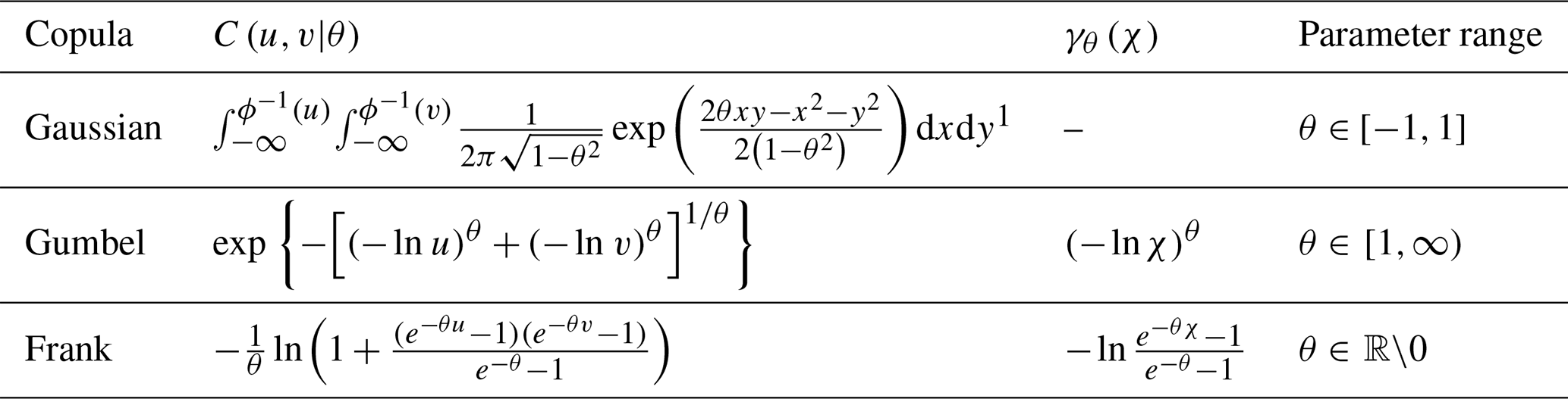
Equation (1) illustrates why copulas are widely used in higher-dimensional statistics, as they enable separate modeling of the marginals and their dependency structure, simplifying the construction of joint distributions. For a more detailed description of the copula theory, the reader is referred to Joe (1997) and Nelsen (2006). In this study we considered three well-established types of copulas (Table 1):

1. Gaussian copula. In this copula, the joint probability density function exhibits symmetry around a central point, with the contours of constant density forming ellipsoids in the multivariate space. The Gaussian copula models situations where the dependency structure between two variables remains constant across the entire distribution and does not exhibit tail dependence.

2. Gumbel copula. This is an Archimedean copula, i.e. it models the dependencies among variables using a function of the marginal probability, called “generation function”, able to capture non-linear dependencies. In particular, the Gumbel copula can adequately reproduce conditions when the dependency among variables is stronger for the upper tails. For higher-dimensional cases (trivariate and above), we use a C-vine construction, which builds the multivariate dependence from pairwise Gumbel copulas in a hierarchical tree structure.

3. Frank copula. This is an Archimedean copula that suits situations that are tail-independent in both tails, meaning that as values approach extreme highs or lows, the dependence between them weakens.

Table 1 List of copula functions implemented in tsEVA 2.0. In the table, the symbol ϕ() represents the standard normal distribution. For Archimedean copulas (e.g., Gumbel and Frank) γ_θ(χ) denotes the generator function used in constructing the copula $C\left(u,v\mathrm{|}\mathit{\theta }\right)={\mathit{\gamma }}_{\mathit{\theta }}^{-\mathrm{1}}\left[{\mathit{\gamma }}_{\mathit{\theta }}\left(u\right)+{\mathit{\gamma }}_{\mathit{\theta }}\left(v\right)\right]$.

To describe the time evolution of the copula, we evaluated a time-varying coupling parameter θ_t on a moving window, similar to what proposed by Li et al. (2019). The duration of series is covered by N time windows where:

$$\begin{array}{}\text{(2)}& N=⌊{\displaystyle \frac{T-w}{\mathrm{\Delta }t}}⌋+\mathrm{1}\end{array}$$

where T is the length of the series (in years), w is the window length (in years), Δt=1 is the window shift (sliding by 1 year), and N is the number of moving windows. The symbol ⌊⌋ ensures a floor operation.

2.2 Non-stationary marginals

The treatment of the marginals (i.e., the distributions of the univariates, $F_{\mathrm{1}},\mathrm{\dots },F_m$ in Eq. 1), was performed in accordance with the univariate theory of extremes. There are two popular approaches that are used to model extremes of a series. The Fisher-Tippett-Gnedenko theorem establishes the Generalized Extreme Value (GEV) distribution as the appropriate distribution for statistically homogeneous block maxima, such as annual maxima. The cumulative GEV distribution is defined as:

$$\begin{array}{}\text{(3)}& {\mathrm{GEV}}_X\left(x;\mathit{\epsilon },\mathit{\mu },\mathit{\sigma }\right)=\exp \left\{-{\left[\mathrm{1}+\mathit{\epsilon }\left({\displaystyle \frac{x-\mathit{\mu }}{\mathit{\sigma }}}\right)\right]}^{-\mathrm{1}/\mathit{\epsilon }}\right\},\end{array}$$

where ε, μ, and σ are the shape, location and scale parameters, that need to be found out through a fitting process. On the other hand, the Generalized Pareto Distribution (GPD) is the general form of the distribution of the Peaks Over Threshold (POT) according to the Pickands–Balkema–De Haan theorem. The cumulative GPD is defined as

$$\begin{array}{}\text{(4)}& {\mathrm{GPD}}_{X-u}\left(\stackrel{\mathrm{̃}}{x};\mathit{\epsilon },\stackrel{\mathrm{̃}}{\mathit{\sigma }}\right)=\mathrm{1}-{\left(\mathrm{1}+{\displaystyle \frac{\mathit{\epsilon }\stackrel{\mathrm{̃}}{x}}{\stackrel{\mathrm{̃}}{\mathit{\sigma }}}}\right)}^{-\mathrm{1}/\mathit{\epsilon }},\end{array}$$

where $\stackrel{\mathrm{̃}}{x}=x-u$ is the series of excess values relative to the selected threshold value (u), and ε and $\stackrel{\mathrm{̃}}{\mathit{\sigma }}$ are the shape and scale parameters respectively (Coles, 2001).

To address non-stationarity in the marginal distributions, we adopted the approach proposed by Mentaschi et al. (2016), which demonstrates that a transformation formally equivalent to local normalization allows for a generalized representation of non-stationary extreme value distributions while maintaining a constant shape parameter. Specifically, the transformation f is defined as:

$$\begin{array}{}\text{(5)}& y\left(t\right)\stackrel{f\left(y,t\right)}{⟶}x\left(t\right)\mathrm{where}f\left(y,t\right)={\displaystyle \frac{y\left(t\right)-T_y\left(t\right)}{C_y\left(t\right)}}\end{array}$$

where y(t) is the non-stationary series, x(t) is the assumed stationary series, T_y (t) and C_y (t) are generic terms representing the long-term variation in the mean and amplitude of y(t), respectively. A back-transformation from the stationary domain x to the non-stationary one y leads to a formulation of parameters of time-varying extreme values distribution. In particular, for the GEV one obtains:

$$\begin{array}{}\text{(6)}& \left\{\begin{array}{l}{\mathit{\epsilon }}_y={\mathit{\epsilon }}_x\\ {\mathit{\sigma }}_y\left(t\right)=C_y\left(t\right)\cdot {\mathit{\sigma }}_x\\ {\mathit{\mu }}_y\left(t\right)=C_y\left(t\right)\cdot {\mathit{\mu }}_x+T_y\left(t\right),\end{array}\right.\end{array}$$

and for the GPD:

$$\begin{array}{}\text{(7)}& \left\{\begin{array}{l}{\mathit{\epsilon }}_y={\mathit{\epsilon }}_x\\ {\stackrel{\mathrm{̃}}{\mathit{\sigma }}}_y\left(t\right)=C_y\left(t\right)\cdot {\stackrel{\mathrm{̃}}{\mathit{\sigma }}}_x\\ u_y\left(t\right)=C_y\left(t\right)\cdot u_x+T_y\left(t\right).\end{array}\right.\end{array}$$

2.3 Joint sampling of the extremes

There are several methods to sample joint extremes from multivariate data (e.g., Zheng et al., 2014). The simplest method used in tsEVA 2.0 applies a block-maxima technique, compatible with GEV-distributed marginals, focusing on the coupling of annual maxima from each variable. A key limitation of this method, inherent to the GEV distribution, is that not all extremes are annual maxima, nor are all annual maxima truly extreme events. Additionally, this approach may link events far apart in time while missing those that occur close together but fall across block boundaries. Despite these limitations, its simplicity makes it effective for studying dependencies among relatively slow, seasonal phenomena, such as drought and heat waves.

A more advanced approach involves non-stationary joint Peaks Over Threshold (POT) sampling. This method first applies the transformation in Eq. (4) to convert each non-stationary signal y(t) to a stationary series x(t). POT sampling is then conducted on each stationarized series x(t), selecting multivariate peaks within a defined maximum time interval Δt_multivariate. A challenge with this approach is the potential for multiple combinations of univariate peaks within the interval Δt_multivariate. In tsEVA 2.0, this issue is addressed by prioritizing joint peaks with the largest mean values (average of univariate peak values), iteratively removing all other peak combinations.

2.4 Goodness-of-fit

To evaluate the goodness-of-fit (GOF) of the copula model, a multi-parameter approach was employed by analyzing a set of statistics that quantify the similarity between the fitted distribution and the empirical data. Specifically, the following statistics were considered:

Cramér-von Mises statistic. Its general definition is:

$$\begin{array}{}\text{(8)}& S_n=\int {\left[C_n\left(u\right)-C_{\mathit{\theta }}\left(u\right)\right]}^{\mathrm{2}}\mathrm{d}u,\end{array}$$

where C_n is the empirical distribution, C_θ is the theoretical fit, u is defined in the domain of the distributions. The statistic S_n serves as a proxy for the distance between the empirical and theoretical distributions in probability space. In this study, we applied the rank-based version of the Cramér-von Mises statistic (Genest et al., 2009), where the ranks of C_n and C_θ are compared using Monte Carlo simulations. For non-stationary distributions, S_n is estimated separately over different time windows, and the results are averaged, to provide the mean Cramér-von Mises statistic $\stackrel{\mathrm{‾}}{S_n}$.

For each bivariate sub-distribution, the goodness-of-fit was evaluated by comparing the correlation structure of the fitted copula to that of the original data. Specifically, the differences in Spearman's rank correlation coefficient (Δρ_Spearman) and Kendall's tau (Δτ_Kendall) were computed between a Monte Carlo simulation of the fitted copula distribution and the empirical values derived from the original sample. This provides a measure of how well the fitted model captures the dependency structure of the data. For multivariate non-stationary copulas, this analysis was extended by computing the average differences Δρ_Spearman and Δτ_Kendall over all the bivariate sub-distributions and the considered time windows. The metrics are defined as:

$$\begin{array}{}\text{(9)}& {\displaystyle }{\stackrel{\mathrm{‾}}{\mathrm{\Delta }\mathit{\rho }}}_{\mathrm{Spearman}}={\displaystyle \frac{\mathrm{1}}{N\cdot P}}\sum _{t=\mathrm{1}}^N\sum _{\mathrm{1}\le i<j\le d}\left|{\mathit{\rho }}_{t,(i,j)}-{\mathit{\rho }}_{t,(i,j),\mathrm{MC}}\right|\text{(10)}& {\displaystyle }{\stackrel{\mathrm{‾}}{\mathrm{\Delta }\mathit{\tau }}}_{\mathrm{Kendall}}={\displaystyle \frac{\mathrm{1}}{N\cdot P}}\sum _{t=\mathrm{1}}^N\sum _{\mathrm{1}\le i<j\le d}\left|{\mathit{\tau }}_{t,(i,j)}-{\mathit{\tau }}_{t,\left(i,j\right),\mathrm{MC}}\right|\end{array}$$

where ${\mathit{\rho }}_{t,(i,j)}$ and ${\mathit{\rho }}_{t,(i,j),\mathrm{MC}}$ are the Spearman correlation of variables i and j at time window t for the original and Monte-Carlo samples, $P=\frac{d\cdot (d-\mathrm{1})}{\mathrm{2}}$ is the total number of bivariate pairs, d is the total number of variables, N is the total number of windows, ${\mathit{\tau }}_{t,(i,j)}$ and ${\mathit{\tau }}_{t,\left(i,j\right),\mathrm{MC}}$ are the Kendall correlation of variables i and j at time window t for the original and Monte-Carlo samples, and ${\stackrel{\mathrm{‾}}{\mathrm{\Delta }\mathit{\rho }}}_{\mathrm{Spearman}}$ and ${\stackrel{\mathrm{‾}}{\mathrm{\Delta }\mathit{\tau }}}_{\mathrm{Kendall}}$ are the absolute difference in Spearman and Kendall correlation averaged across time windows and across bivariate pairs of variables.

2.5 Bivariate Return Periods

In the non-stationary context, there is not any standard definition of a return period, and different propositions have been made (Yan et al., 2017). Therefore, the interpretation of return periods requires careful definition, and different frameworks have been proposed (Parey et al., 2010; Yan et al., 2017). In Parey et al. (2010), univariate return levels are computed for the stationary transformed variable and then back-transformed to represent a specific target future climate period. The tsEVA framework adopts a similar transformation-based philosophy but with a different implementation and interpretation.

Multivariate return periods can be defined in several ways (Serinaldi, 2015; Salvadori et al., 2016). In tsEVA 2.0, we adopted the following two definitions:

A definition that is more relevant in risk analysis and represent simultaneous exceedance of variables over their given thresholds (the AND return period) which for bivariate case, reads as:

$$\begin{array}{}\text{(11)}& T_{u\mathrm{1},u\mathrm{2}}^{\mathrm{AND}}={\displaystyle \frac{\mathit{\mu }}{\mathrm{1}-u_{\mathrm{1}}-u_{\mathrm{2}}+C\left(u_{\mathrm{1}},u_{\mathrm{2}}\right)}}\end{array}$$

A definition that is closest to the definition of cumulative multivariate distribution function (the OR return period) which for the bivariate case, reads as:

$$\begin{array}{}\text{(12)}& T_{u\mathrm{1},u\mathrm{2}}^{\mathrm{OR}}={\displaystyle \frac{\mathit{\mu }}{\mathrm{1}-C\left(u_{\mathrm{1}},u_{\mathrm{2}}\right)}}\end{array}$$

where μ is the average inter-arrival time, representing the mean time between peaks and $u_i=F_{X_i}\left(x_i\right)$ represents continuous marginal distributions. The OR return period ($T_{u\mathrm{1},u\mathrm{2}}^{\mathrm{OR}}$) refers to the case where at least one of the x_i values is exceeded while the AND return period $T_{u\mathrm{1},u\mathrm{2}}^{\mathrm{AND}}$ represent the case where both of the variables have exceeded x_i values. In bivariate analysis, joint probabilities associated with return periods form level curves (also known as isolines). Based on the above definition, we restricted the use of joint return periods to bivariate cases only. In the non-stationary context, return periods are conditional on the statistical properties (marginals and dependence) of each time window. The computation procedure is as follows: For each time window, we estimate (i) the time-varying marginal distributions from the back-transformed non-stationary GEV or GPD parameters, and (ii) the copula function C(u,v) from the coupling parameter specific to that window. These are combined using the AND and OR definitions (Eqs. 7 and 8) to compute joint exceedance probabilities.

2.6 Detection of non-stationarity

The Mann-Kendall (MK) test is a nonparametric method used to detect trends in data over time. It compares pairs of data points to identify a consistent upward or downward trend. After calculating a test statistic, a p-value is obtained and compared to a chosen significance level (α) to determine whether the trend is statistically significant. A p-value below α indicates a significant trend, while a larger p-value suggests the trend is not statistically significant. A commonly used value for α is 0.05, but it can be adjusted depending on the context and requirements of the analysis.

We used MK to assess non-stationarity of the univariate marginals by applying the test on the annual percentile series. To see the effectiveness of transformation, the test was applied on both stationary and non-stationary series (i.e., before and after application of transformation). This method was applied as a shortcut to other sophisticated tests for stationarity that rely on bootstrapping (e.g., Parey et al., 2013).

To assess the non-stationarity of the joint distribution, we applied the modified Mann–Kendall test (Hamed, 2008; Hamed and Rao, 1998; Yue and Wang, 2004), which explicitly accounts for autocorrelation arising from the 1-year sliding window used to compute the temporal evolution of the coupling parameter. By considering this autocorrelation, the test provides a more accurate assessment of statistical significance, avoiding the overestimation of trend significance that can occur with overlapping windows.

2.7 Assembling the Pieces: the tsEVA 2.0 toolbox

The methodologies outlined above are integrated into a MATLAB toolbox tsEVA 2.0, an extension of the original tsEVA by Mentaschi et al. (2016), providing a versatile framework for multivariate analysis of non-stationary extremes across various applications. The toolbox features two primary functions: one employing non-stationary multivariate POT sampling with GPD and the other utilizing multivariate block-maxima sampling with GEV (Fig. 1).

Figure 1 Flowchart of tsEVA 2.0.

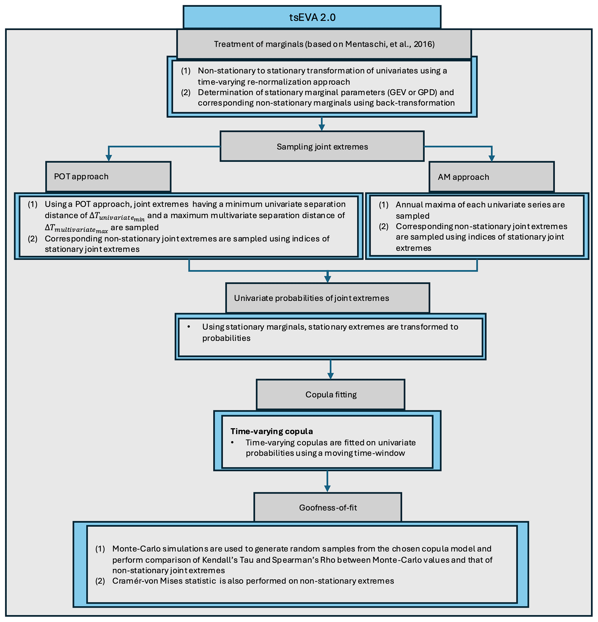
In both approaches, the analysis begins by applying tsEVA's method to transform each univariate time series from non-stationary to stationary. The extreme value distribution (either GPD or GEV) is then fitted to the stationary series, and the resulting distributions are back-transformed into the time-varying domain to represent the non-stationary marginals. Joint extremes are subsequently sampled and mapped into probability space using the stationary marginals. A copula is then fitted to this transformed dataset, which can either be stationary (assuming constant dependency over time) or non-stationary (accounting for time-varying dependency). To ensure the appropriateness of each copula model in representing the joint distribution of non-stationary extremes, we developed a dedicated goodness-of-fit routine. A flowchart of tsEVA 2.0 is presented in Fig. 1.

2.8 Case studies

To demonstrate the applications of the general method developed for analyzing non-stationary joint extremes, the methodology was applied to three case studies, each selected to highlight specific features of the new methodology. All the data in the following examples were obtained from model results. Possible biases in the model data can also find its way into quantification of return periods. Nonetheless, these model outputs provided a good basis upon which the general methodology developed in this paper could be substantiated. For the wave dataset used in the first and second case study, we used a bias-corrected version of the results reported in Mentaschi et al. (2023). The bias correction was based on Quantile mapping, and we focused on values above 50th percentile. The bias-correction was based on comparison with satellite measurements.

2.8.1 Joint extremes of river discharge and wave height

This case study explored the evolving relationship between river discharge and significant wave height (SWH) near the coast over time. The focus was on the mouth of the La Liane River in France, a fast-responding river influenced by precipitation. Wave data comprised 3 h SWH records from a high-resolution global wave model (Mentaschi et al., 2023) with nearshore resolutions of 2–4 km, covering the period 1950–2020. River discharge data was obtained from the HERA hydrological reanalysis (Tilloy et al., 2025). The dataset, generated with the OS LISFLOOD model (Burek et al., 2013), provides high resolution (approx. 1.5 km) simulation of river discharge for every river with an upstream area >100 km² across Europe.). The data comes at 6 h records over the same time frame. Although residual model biases contribute to uncertainty in return level estimation, the use of model data for coastal hazard mapping is widely established practice, as models provide complete spatiotemporal coverage that cannot be achieved through sparse observational networks. The wave dataset employed in this study (Mentaschi et al., 2023) was post-processed to reduce biases through quantile mapping against satellite observations. Likewise, the river discharge dataset (Tilloy et al., 2025) was evaluated using 2448 river gauging stations to assess model skill.

The analysis used the Generalized Pareto Distribution (GPD) for univariate margins and a time-varying Gumbel copula to model dependence. Univariate peaks were selected with a minimum separation of 30 d. In this case study, joint extremes were defined as events in which the peak of river discharge occurred within a maximum time lag of 45 d after the peak of wave height. The choice of a 45 d maximum allowable lag among bivariate peaks reflects the time-lag among univariate peaks (30 d) and the impact-based temporal compounding perspective (Zscheischler et al., 2020): when an extreme sea level event compromises coastal system capacity, a subsequent extreme river discharge within 45 d can produce amplified impacts even without direct hydrodynamic interaction. Following sampling, the average temporal separation among bivariate peaks was approximately 15 d. Non-stationarity of the joint distribution was assessed within a 40-year moving window, with thresholds set at the 95th percentile for river discharge and the 99th percentile for wave height. On average, each 40-year window contains 66 joint extremes, which provides adequate sample sizes for stable copula parameter estimation.

2.8.2 Spatial correlation of extreme wave heights across three locations

The second case study evaluated the spatial relationship of SWH across three locations scattered around the Marshall Islands, using the same source for wave dataset as the first case study. This trivariate analysis highlighted spatial dependencies, employing a non-stationary Gumbel copula with non-stationary margins, modeled with GPD. Each variable was sampled at the 99th percentile, with univariate peaks spaced a minimum of 12 h apart and a maximum allowable distance of 12 h for multivariate peaks. A 40-year time window was used for the joint distribution. Each time window contained 76 joint extremes on average.

2.8.3 Joint Distribution of Surface Temperature and SPEI

The third case study examined the relationship between surface temperature and the 6-month Standardized Precipitation-Evapotranspiration Index (SPEI) in a region south of Milan, Italy (45.25° N, 9.25° E). Hourly surface temperature data from the ECMWF ERA-5 dataset (1959–2023) was paired with monthly SPEI data (1959–2022) (Zhang, 2023). To better capture heatwave dynamics, the temperature data were smoothed using a 10 d running mean. The analysis was restricted to the period from April to September, which aligns with the growing season when drought impacts are at their peak and heatwaves present a significant hazard. This case study demonstrated a scenario where block-maxima sampling is a valid and simpler alternative to the POT method for analyzing extremes. A 35-year non-stationary time window was used in this analysis for the joint distribution.

3 Results

3.1 Case study 1: joint extremes of river discharge and wave height

The non-stationarity of both time series was assessed using the Mann-Kendall test, which revealed significant increasing trends in both variables (Fig. 2a, b). The effectiveness of transformation was verified by p-values both before and after transformation (Fig. 2a, b). Among the evaluated copula models, the Gumbel copula was the best fit for representing the dependence structure with this copula's goodness of fit parameters presented in Fig. 2c. Applying a time-varying Gumbel copula with a 40-year moving window revealed a statistically significant increasing trend in the dependency parameter, denoted as θ_Gumbel (Fig. 1c). A similar upward trend was observed in the Spearman correlation coefficient ρ_Spearman, calculated for both the sampled joint extremes and Monte Carlo-generated samples.

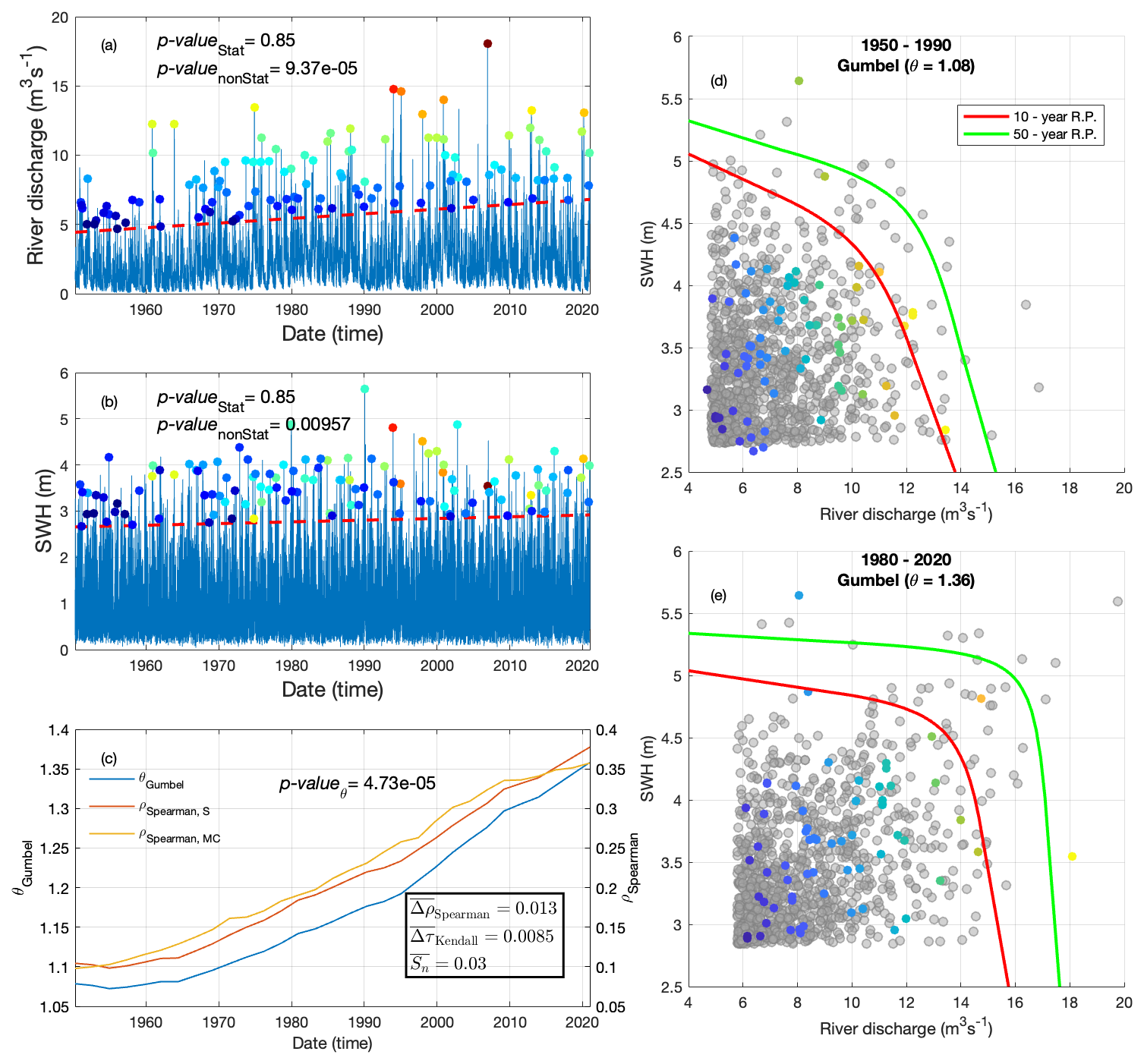
Figure 2 Analysis of joint extremes of river discharge and wave height off La Liane river mouth. In panels (a) and (b) the input series are presented (blue line). The thick dashed red line is the time-varying threshold level while the colored dots indicate the joint extreme events. The color of dots was based on events having the largest mean value. Also shown in these two plots is the p-value of Mann-Kendall test of the percentile series applied on both stationary (denoted by Stat) and non-stationary (denoted by nonStat) series. Variation with time of the copula parameter was depicted in panel (c) with a p-value of Mann-Kendall test. Other goodness-of-fit parameters of the non-stationary copula model were shown in panel (c). A 10-window smoothing was applied to curves of panel (c) for better representation. The time-varying Spearman correlation coefficient of the samples (red line) and Monte-Carlo values (yellow line) were also presented in panel (c). Panels (d) and (e) present the overlay of joint extremes (colored dots) and Monte-Carlo values (gray dots) in two different time windows (1950–1990) of (1980–2020) with the copula parameter indicated above. The 10 and 50-year joint return levels (using the AND definition) are also shown in these panels (colored curves).

To illustrate these findings, two representative time windows were selected, comparing the theoretical Gumbel copula (gray dots, based on Monte Carlo simulations) with the sampled joint extremes (Fig. 2d, e). These panels visually confirmed a stronger coupling between the two variables toward the end of the time series. This increase of coupling was also evident in shape of level curves corresponding to 10 and 50-year return periods. Furthermore, the analysis of joint return periods revealed substantial shifts in level curves between the beginning and end of the series (curves in Fig. 2d–e), demonstrating the utility of this technique in capturing temporal variations (non-stationarity) in joint extremes.

3.2 Case study 2: trivariate joint extremes of significant wave height

The co-occurrence of extreme SWH at three locations (P1–P3) around the Marshall Islands was examined as the second case study (Fig. 3). Univariate non-stationarity was evaluated using the Mann-Kendall test (Fig. 3b, f, i), which revealed the strongest non-stationarity at P2, as indicated by its lowest p-value. Both P1 and P3 also exhibited positive trends, significant at the 90 % confidence level. The effectiveness of transformation for each bivariate pair was assessing by comparing p-values before and after transformation (Fig. 3b, f, i). The transformation clearly influenced the detected trends with all pairs showing p-values greater than 0.7 after the stationarizing step.

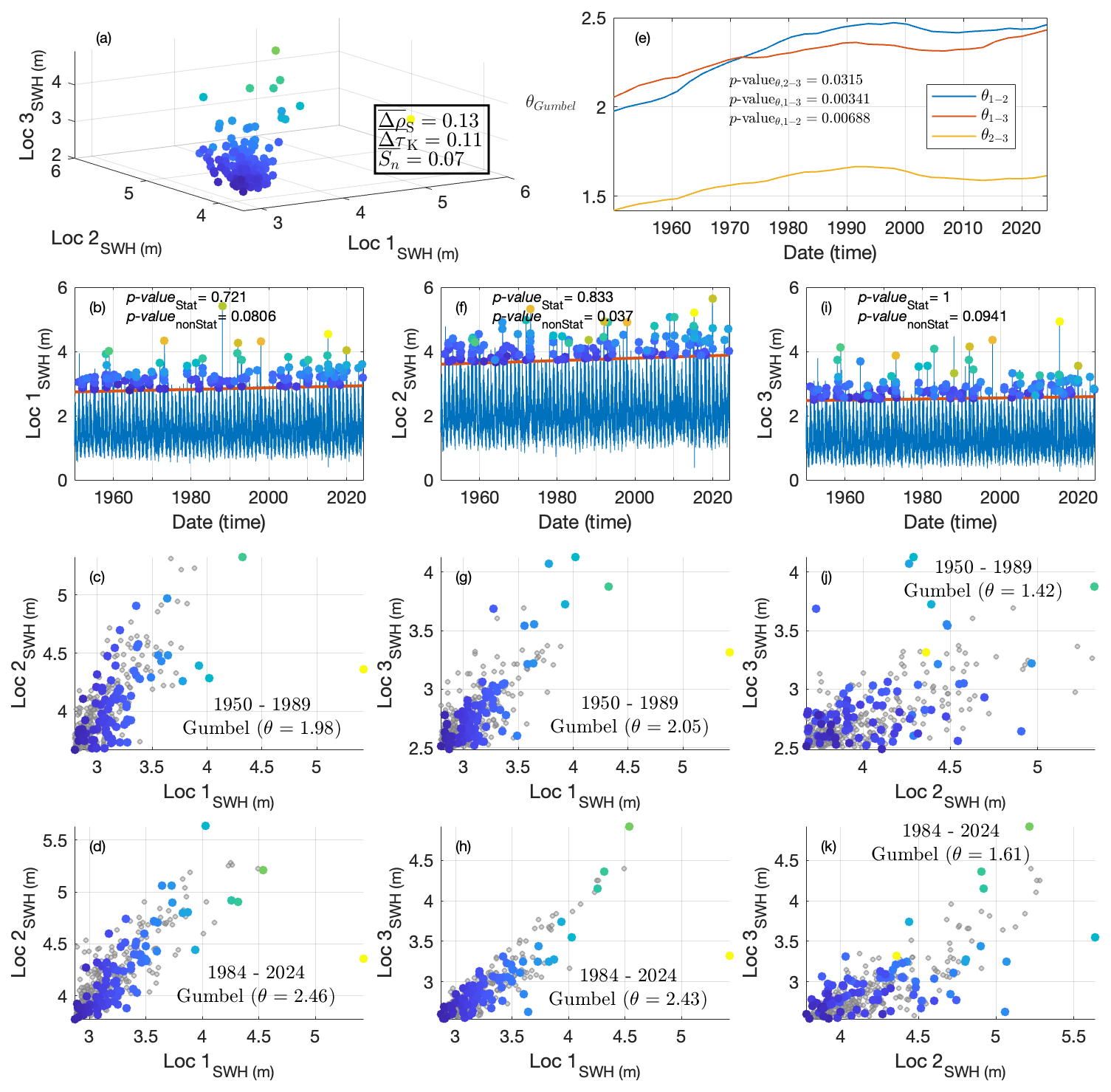
Figure 3 Analysis of trivariate extremes of SWH in neighboring locations near Marshall Islands. Goodness-of-fit parameters and sampled extremes are presented in panel (a). Univariate extremes (colored dots) and threshold levels (thick red lines) along with the p-value of the Mann-Kendall test of the percentile series applied on both stationary (denoted by Stat) and non-stationary (denoted by nonStat) series are presented in panels (b), (f) and (i). Panels (c), (d), (g), (j), (k) and (i) present overlaying of pairs of extremes (colored dots) and Monte-Carlo values (gray dots) with the copula parameter and time window indicated above each panel. The time-varying coupling parameter of each pair of extremes and the p-value of the Mann-Kendall test of the coupling parameter is presented in panel (e). A 10-window smoothing was applied to curves of panel (e).

Non-stationarity in the coupling was evaluated using a time-varying Gumbel copula model, showing significant increasing trends in correlation for all pairs (p-value <0.05) (Fig. 3e). Notably, the correlations for P1–P3 and P1–P2 have p-values near zero, whereas the correlation for P2–P3 is approximately 0.03 (Fig. 3e). The pairs of extremes of SWH exhibited a change in correlation with time, with the Gumbel coupling parameter changing from 1.98 to 2.46 for P1–P2 pair, 2.05 to 2.43 in P1–P3, and 1.42 to 1.61 in P2–P3 (Fig. 3c, d, g, h, j, k). The Monte Carlo extractions (gray dots in Fig. 3c, d, g, h, j, k) closely matched the data samples, demonstrating good agreement. The goodness-of-fit metrics indicated accurate results, with ${\stackrel{\mathrm{‾}}{\mathrm{\Delta }\mathit{\rho }}}_{\mathrm{Spearman}}=\mathrm{0.13}$, ${\stackrel{\mathrm{‾}}{\mathrm{\Delta }\mathit{\tau }}}_{\mathrm{Kendall}}=\mathrm{0.11}$, $\stackrel{\mathrm{‾}}{S_n}=\mathrm{0.07}$ (Fig. 3a).

3.3 Case study 3: joint extremes of surface temperature and SPEI

The final case study examines joint extremes of surface temperature and the SPEI at an inland location south of Milan, focusing on the period from April to September. In this case, an annual maxima sampling technique was employed to identify univariate extremes (Fig. 4a, b), and the Gumbel copula was used to model their joint distribution. Consequently, the marginals were estimated using the GEV distribution.

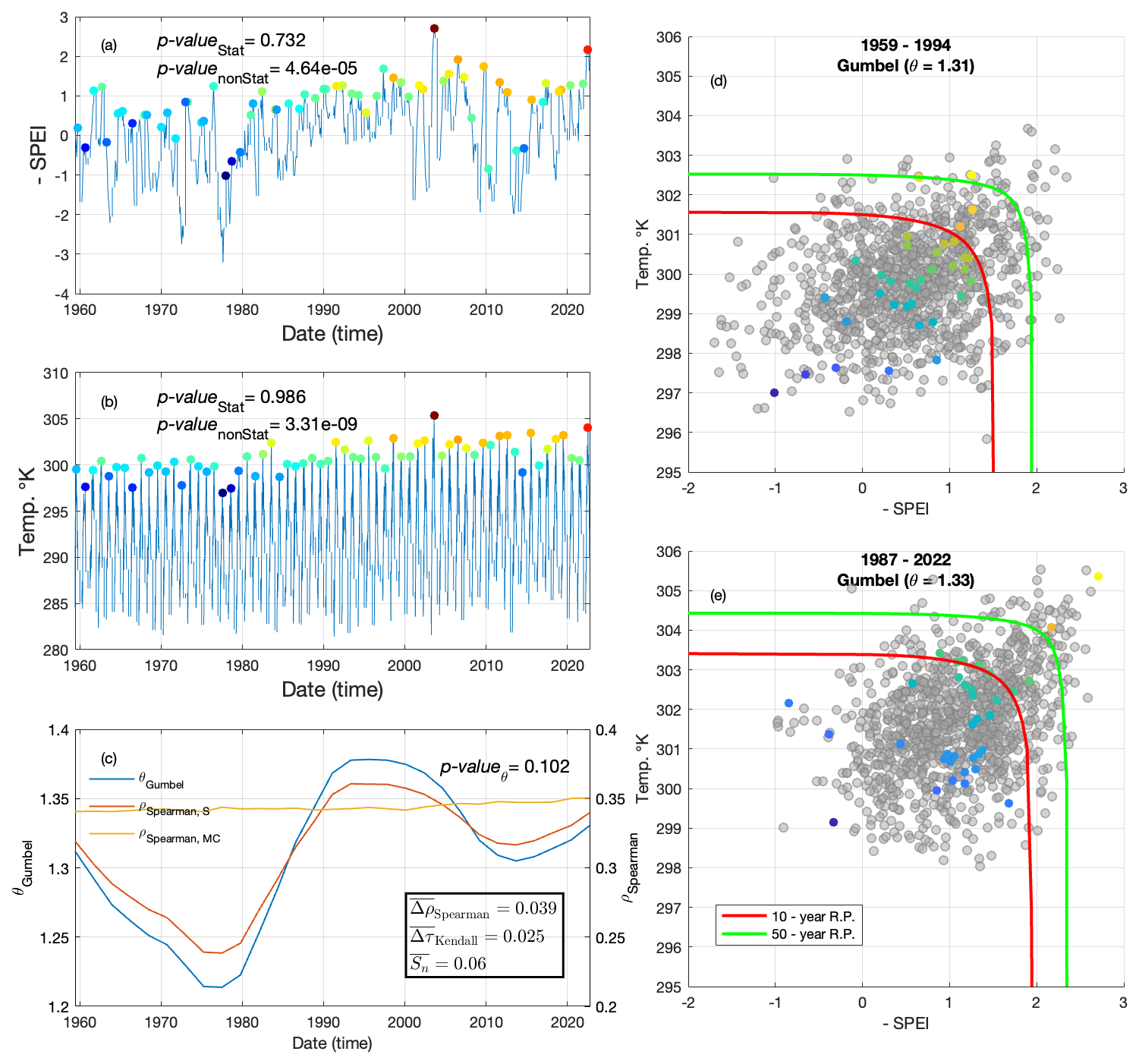
Figure 4 Analysis of annual extremes of SPEI and temperature (° C). Panels (a) and (b) display the input series (thin blue line) alongside the annual maxima (colored dots), where SPEI values have been multiplied by −1 for interpretability. The color of the dots reflects the mean values of the joint extremes. The p-value from the Mann-Kendall test applied on both stationary (denoted by Stat) and non-stationary (denoted by nonStat) series for the annual maxima is also reported in these panels. Panel (c) presents the goodness-of-fit parameters for the copula model, along with the time-varying coupling parameter (left axis) (thick blue line) and the time-varying Spearman correlation coefficient, calculated for both the original samples and the Monte Carlo values (right axis). A 10-window smoothing was applied to curves of panel (c) for better representation. Panels (d) and (e) overlay the joint extremes (colored dots) with Monte Carlo values (gray dots), simulated based on the constant coupling parameter specified in each panel. The level of agreement between the observed and simulated values demonstrates the validity of the fitted copula model. Also shown in these two panels is the joint return levels (using AND definition) corresponding with the 10 and 50-year return levels (colored curves).

Non-stationarity in both series was assessed through the Mann-Kendall test, with p-values close to zero (Fig. 4a, b). The p-values increased significantly after the transformation based on comparison of p-values obtained from original non-stationary and transformed stationary series (Fig. 4a, b). Based on goodness-of-fit statistics (${\stackrel{\mathrm{‾}}{\mathrm{\Delta }\mathit{\rho }}}_{\mathrm{Spearman}},{\stackrel{\mathrm{‾}}{\mathrm{\Delta }\mathit{\tau }}}_{\mathrm{Kendall}}$ and $\stackrel{\mathrm{‾}}{S_n})$, the Gumbel copula was identified as the best-performing model for representing the joint distribution of extremes (Fig. 4c). The application of a non-stationary Gumbel copula allowed for the estimation of a time-varying coupling parameter (blue curve in Fig. 4c). However, unlike the previous two examples, no significant trend was detected in the time-varying coupling parameter (Fig. 4c). This indicates that the non-stationarity in the joint distribution was solely driven by the non-stationarity of the marginals. The Spearman correlation parameter of the joint extremes also indicated lack of significant trend (red line; Fig. 4c). Thus, in this example a constant coupling parameter was adopted (mean of the blue curve in Fig. 4c). Subsequently, the Monte-Carlo samples generated based on the coupling parameter indicated near-constant Spearman correlation parameter (yellow line; Fig. 4c). The evolving interrelationships of extremes was also verified by a visual inspection of different time windows across the duration of series (Fig. 4d, e). Evidently, the Gumbel copula was a good representation for co-occurrences of extremes, where stronger dependencies was observed in the upper tail of both time windows (Fig. 4d, e). The non-stationarity of the marginals resulted in change of level curves corresponding with 10 and 50-year joint return periods (colored curves in Fig. 4d, e).

4 Discussion

Extreme Value Analysis (EVA) is a robust and widely used method for estimating the frequency of rare and impactful events. However, the growing availability of long-term, large-scale time series for hazard-related variables, from both historical and climate studies, has increasingly demonstrated that the assumption of stationarity, a cornerstone of EVA, often does not hold. In the case studies examined in this research, statistically significant trends were observed across all the time series analyzed. Moreover, beyond significant temporal changes in the extremes of many univariate series, clear non-stationarity was also observed in the dependencies between different variables. This study highlights the importance of considering non-stationarity in modeling joint distribution of natural hazard data.

The first case study explores the relationship between river discharge and coastal hazard-related variables, such as significant wave height (SWH). While the coupling between these variables is relatively weak, it remains statistically significant, indicating that the likelihood of compound events is higher than would be expected if the variables were independent. Among the three tested copula models, the Gumbel copula demonstrated the best fit, capturing the stronger dependency observed in the upper tails. The analysis of the Liane River discharge and the SWH near its mouth over the past 70 years reveals a significant upward trend in both variables, as evidenced by p-values approaching zero (Fig. 2a, b). Correspondingly, the coupling parameter has shown a marked increase over time, with the Spearman correlation rising from less than 0.1 in 1950 (a low but statistically significant value) to over 0.37 in 2020 (Fig. 2c). This growing interdependence has led to a pronounced upward shift in the AND return level curves (Fig. 2d, e). This significant growth in coupling may be attributed to two factors: the inherent stronger upper-tail dependency captured by the Gumbel copula and the increasing frequency of extreme values in both river discharge and SWH. These findings suggest that while the underlying dynamics of the coupling have remained stable, the amplification of extremes in both variables have intensified their overall interdependence during joint peak events.

The second case study investigates the spatial dependency of extremes in a hazard-related variable, specifically significant wave height (SWH). This aspect is critical for risk assessment, as hazards often exhibit strong spatial coherence. When an extreme event, such as a severe storm, impacts one location, it is highly likely to affect neighboring areas as well. Consequently, hazards at different locations cannot be assumed to be statistically independent (e.g., Vousdoukas et al., 2020). Previous studies have examined spatial dependencies of extreme SWH using satellite altimeter observations or sparse buoy data (e.g., Shooter et al., 2021; Jane et al., 2016; Wang et al., 2024). These works aimed to quantify spatial dependence in extreme wave events, offering valuable insights for coastal inundation studies and the creation of hazard maps. In this case study, high-resolution numerical wave model data from Mentaschi et al. (2023) were employed to assess the spatial correlation of extreme SWH, accounting for non-stationarity in the marginal distributions and coupling intensity. The analysis focused on three locations near the Marshall Islands, approximately 250 km apart for P1–P2 and P1–P3, and 350 km apart for P2–P3. These locations are in a region characterized by numerous small islands that act as natural barriers, attenuating wave energy from certain directions. Despite these geographical features, the dependency between the variables remains significant. The degree of coupling in extreme SWH among the three locations shows a clear relationship with their spatial separation. The comparable distances between P1–P2 and P1–P3 correspond to similar levels of dependency in extreme wave events, with correlation values increasing from 1.98 and 2.05 at the start of the time series to 2.46 and 2.43 by its end, respectively. In contrast, the greater distance between P2–P3 results in a weaker dependency, with correlations starting at about 1.42 and rising to 1.61 over the same period. The growing dependency among SWH at the three locations is supported by the Mann-Kendall test applied to the coupling parameter. The test results indicate a p-value near zero for the pairs P1–P2 and P1–P3, while the pair P2-P3 has a p-value of approximately 0.03. This observed increase in spatial dependency across all pairs suggests that not only have extreme events intensified in the region, but their spatial extent may have also expanded, affecting larger areas over time.

The third case study focuses on two hazard-related variables, temperature (a proxy for heatwaves) and the SPEI, a proxy of drought, in the Milan area of Italy, both of which are strongly influenced by non-stationarity. The coupling between these variables is well-documented, arising from the interplay between temperature-driven evapotranspiration and the development of dry conditions. At the same time, dry conditions lead to reduced evapotranspiration and greater heat accumulation on land surfaces (e.g., Manning et al., 2019). However, previous studies (e.g., Ribeiro et al., 2020) have often overlooked the impacts of non-stationarity when assessing the joint distribution of their extremes.

It is true that the asymptotic justification for the GEV distribution relies on block independence (or weak dependence), and that slowly-varying seasonal phenomena such as droughts and heat waves exhibit temporal correlation structures that may challenge these assumptions. Although SPEI-6 represents a slowly-developing process, the GEV distribution has been shown to provide adequate fits for such variables at appropriate aggregation scales. Stagge et al. (2015) demonstrated that GEV outperformed alternative distributions for SPEI across Europe for accumulation periods from 1 to 12 months. For the moderate temporal aggregations considered here (monthly temperature, SPEI-6), the GEV provides a practical and empirically supported approximation for extreme value analysis. Alternative approaches such as stochastic generation methods (Parey and Gailhard, 2022) may offer additional rigor for specific applications with stronger temporal dependence. Our analysis revealed pronounced non-stationarity in both variables, with p-values from the Mann-Kendall test close to zero (Fig. 4a, b), clearly associated with ongoing climate change and global warming. The Gumbel copula was found to be the most appropriate model for the joint distribution of SPEI and temperature, highlighting their strong coupling during extreme events. Unlike the other two case studies, however, the coupling between these variables lacked a significant trend. This was evidenced by the Mann-Kendall test on the time-varying coupling parameter, which resulted in a p-value of 0.102 (Fig. 4c). Given the low significance of the temporal change in the coupling between temperature and SPEI, this case study presented an application where the joint behavior modelled by a Gumbel copula was mostly influenced by non-stationarity of the marginals.

5 Final remarks

In this study, we extended the methodology for non-stationary Extreme Value Analysis (EVA) proposed by Mentaschi et al. (2016) to enable the modeling of joint distributions of extremes that evolve over time. This advancement addresses a critical limitation of univariate EVA, which cannot account for the interdependence among extremes – a crucial aspect in accurately assessing hazards.

The framework was tested across a set of case studies involving different hazard-related variables, each exhibiting varying degrees of non-stationarity and interdependence. These examples demonstrate the versatility and generality of the methodology, to accommodate a wide range of environmental variables with distinct characteristics in how extremes are sampled and evolve over the long term. Furthermore, the framework includes techniques to evaluate the significance of modeled changes, enhancing its utility for risk assessment.

A remarkable fact is that, in two out of the three case studies, not only do the univariate hazard-related variables exhibit significant temporal changes, but their interdependence also evolves substantially over time. This highlights the importance of adopting a methodology capable of addressing such dynamic relationships, underscoring the relevance of the proposed approach.

Additionally, the framework incorporates built-in tools for Monte Carlo simulations, which are instrumental in evaluating goodness-of-fit and estimating uncertainty. Beyond these applications, these simulations can support a more comprehensive risk analysis by generating statistically consistent hazard scenarios, further extending the utility of the methodology.

To support future research and applications, we have developed an open-source toolbox, tsEVA 2.0, which accompanies this study. The toolbox, along with the data and examples presented in this paper, is freely available online, offering a practical resource for exploring the joint distributions of non-stationary extremes and fostering advancements in hazard and risk assessment.